 Jeffrey G. Dorman1*
 William J. Sydeman1
 Sarah Ann Thompson1
 Joseph D. Warren2
 Helen J. Killeen1
 Brian A. Hoover1
 John C. Field3
 Jarrod A. Santora3,4
- 1Farallon Institute, Petaluma, CA, United States
- 2School of Marine and Atmospheric Sciences, Stony Brook University, Southampton, NY, United States
- 3Fisheries Ecology Division, Southwest Fisheries Science Center, National Marine Fisheries Service, National Oceanic and Atmospheric Administration, Santa Cruz, CA, United States
- 4Department of Applied Math, University of California, Santa Cruz, Santa Cruz, CA, United States
Krill are a direct conduit between primary productivity and recreationally and commercially important higher trophic level species globally. Determining how krill abundance varies with temporal environmental variation is key to understanding their function in coastal-pelagic food webs, as well as applications in fisheries management. We used nine years (2012–19 and 2021) of late spring/early summer hydroacoustic-trawl survey data in the California Current Ecosystem (CCE), coupled with new target strength models of two krill species (Euphausia pacifica and Thysanoessa spinifera), to investigate how adult krill biomass varied during a decade of unusual ocean climate variability. We estimate a mean biomass of 1.75–2.0 million metric tons on the central and northern California continental shelf. Overall, relative krill biomass was ~30% lower during 2015 and 2016, corresponding to a major warming event, and ~30% higher in 2013 and 2018, years of exceptionally strong upwelling. Variation in biomass was related to the prior year’s environmental conditions derived from our seasonal Multivariate Ocean Climate Index (MOCI), and E. pacifica and T. spinifera showed similar covariation during the study period. Biomass co-varied at different spatial scales and across sampling devices, suggesting that multiple indicators of abundance (and dispersion) are available and should be applied in ecosystem monitoring and modeling of krill and krill-dependent predators in the California Current ecosystem.
1 Introduction
The distribution, abundance, and availability of euphausiid crustaceans, hereafter “krill”, is fundamental to marine predator-prey interactions across the globe (Field et al., 2006; Aydin and Mueter, 2007; Szoboszlai et al., 2015; Trathan and Hill, 2016; Cavan et al., 2019). Despite the importance of krill to predatory fish, seabirds, and marine mammals, the effects of environmental variability on the regional abundance of most krill species has yet to be determined. Exceptions to this statement include well-studied populations of Euphausia superba in the Southern Ocean (Brierley et al., 1997; Nicol et al., 2000; Reiss et al., 2008; Atkinson et al., 2009) and Thysanoessa spp. in the Bering Sea (Coyle and Pinchuk, 2002; Ressler et al., 2012) and Barents Sea (Eriksen and Dalpadado, 2011).
The California Current Ecosystem (CCE; ~48°N to 22°N latitude) is a highly productive, yet variable spatially-heterogeneous eastern boundary upwelling system off the west coast of North America (Checkley and Barth, 2009). There is long-held understanding of basic krill species distribution and abundance here (e.g., Brinton, 1962; Brinton and Townsend, 2003) with large basin-scale atmospheric forcing (e.g., Pacific Decadal Oscillation and El Niño Southern Oscillation) impacting regional krill species abundance through advection and changes in in-situ habitat conditions (Marinovic et al., 2002; Brinton and Townsend, 2003; Parés-Escobar et al., 2018; Lilly and Ohman, 2021). In the strongest regions of upwelling in the CCE (northern California, Oregon), seasonal upwelling dynamics also impact regional distribution and abundance through changes in transport (Dorman et al., 2005; Dorman et al., 2015) and primary productivity (Feinberg et al., 2010; Shaw et al., 2010). Recent modeling efforts also provide better insight into oceanographic drivers of krill populations (Dorman et al., 2011; Cimino et al., 2020; Fiechter et al., 2020; Messié et al., 2022).
At least 24 species of krill are known to be “routinely” present in the California Current ecosystem, with many others irregularly observed, and all of them have complex and varying life histories and responses to environmental forcing (Brinton, 1962; Marinovic et al., 2002; Lilly and Ohman, 2021). Of these, Euphausia pacifica and Thysanoessa spinifera are the two numerically dominant krill species of importance to predators in the CCE (e.g., Abraham and Sydeman, 2006; Dufault et al., 2009; Szoboszlai et al., 2015; Nickels et al., 2019). T. spinifera is the more neritic species, occurring primarily over the continental shelf, whereas E. pacifica is most abundant offshore along the continental shelf break and slope (Brinton, 1962; Dorman et al., 2005; Santora et al., 2012). T. spinifera is the larger species (adults up to ~32 mm), contains greater lipid content (Fisher et al., 2020), and is a preferred prey item of predators at certain places and times throughout each year (Abraham and Sydeman, 2006; Wells et al., 2012; Nickels et al., 2019). In contrast, smaller E. pacifica (adults up to ~25 mm) is more abundant and widely distributed (Brinton, 1967; Brinton and Townsend, 2003). Consequently, most studies indicate that E. pacifica and T. spinifera are by far the most numerically abundant and most important species with respect to trophic interactions in this region as well as other regions of the California Current (e.g., Croll et al., 2005; Abraham and Sydeman, 2006; Sakuma et al., 2016; Evans et al., 2021).
Modeled estimates of select species of krill abundance at the ecosystem scale are available from mass-balance models such as ECOPATH and ECOSIM (Christensen and Pauly, 1992; Christensen and Walters, 2004) and Atlantis (Weijerman et al., 2016), but these estimates are typically based on “top-down” estimates of predator consumption needs rather than empirical estimates of actual abundance, and the dynamic models rarely account for the “bottom-up” ecosystem dynamics that are more likely to result in year-to-year changes in abundance. Improved understanding of krill abundance relative to environmental variation is needed to model the effects of food resource availability on predator demography and managed commercial and recreational fisheries. Regional-scale catch per unit effort of krill has been empirically evaluated in relation to seasonal variability in ocean climate (Sydeman et al., 2013; Santora et al., 2014; Ralston et al., 2015), but no study of biomass has been conducted at the ecosystem scale to date.
The objective of this study is to investigate how the abundance of T. spinifera and E. pacifica adults (generally ≥12 mm length) varies interannually over a 10-year period of substantial environmental variation, 2012 through 2021 (no acoustic data were collected in 2020). We focus on the region from Cape Mendocino (40°N) to Pt. Conception (35°N), California (Figure 1), where coastal upwelling is strongest (Checkley and Barth, 2009), and where our acoustic-trawl survey effort was concentrated (Santora et al., 2011a, Santora et al., 2018). To estimate adult krill biomass, we applied a target strength model to hydroacoustic data (Warren and Lucca, 2020; Warren et al. in prep), and length-frequency measurements from concurrent trawls (Killeen et al., 2022). This study was conducted during a period characterized by extreme oceanographic conditions, including record coastal upwelling in 2013 (Leising et al., 2014) and 2018 (Thompson et al., 2018; Thompson et al., 2019), and an unprecedented marine heat wave in 2014–15 (Bond et al., 2015), followed by strong El Niño Southern Oscillation (ENSO) conditions in 2016 (Di Lorenzo and Mantua, 2016). Here we compare krill biomass estimates to the Multivariate Ocean Climate Index (MOCI; www.faralloninstitute.org/moci; Sydeman et al., 2014; García-Reyes and Sydeman, 2017) to test the hypothesis that krill biomass declines/increases during periods of weak/strong upwelling and warm/cool temperatures, and to determine the environmental effects on krill biomass.
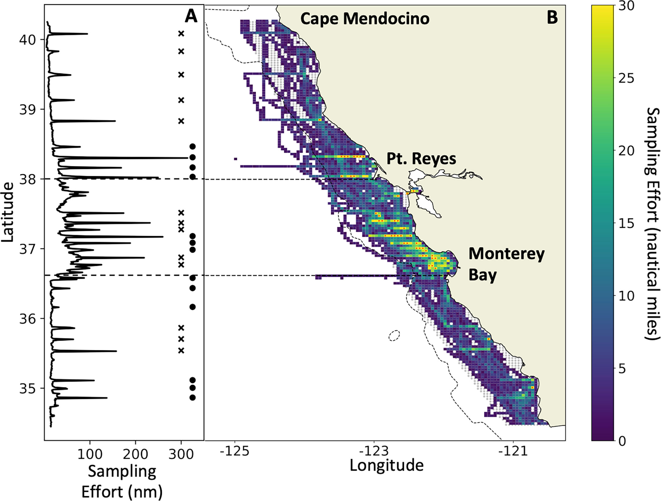
Figure 1 Acoustic sampling effort (nautical miles surveyed per grid cell) on the 2012–2021 RREAS between Cape Mendocino and Pt. Conception (A) by latitude, and (B) spatially explicit. Horizontal dashed lines delineate the core region defined in the text. Gray shading (in B) represents the spatial extent of the grid (~60 km offshore) used to calculate biomass for the region. Adjacent stars and circles (in A) identify latitudinal transect lines and how they were grouped for analysis. Grid cells with a red marker (in B) exceed the maximum number of nautical miles set by the color scale. The maximum number of nautical miles sampled in any grid cell was 88.5 nmi.
2 Materials and methods
2.1 Survey background
Acoustic and trawl data were collected as part of the NOAA-NMFS Rockfish Recruitment and Ecosystem Assessment Survey (RREAS; Sakuma et al., 2016). The RREAS is an annual survey of continental shelf and slope habitat off California that typically occurs over ~45 days from late April to mid-June each year. A complete map of all trawl stations from the RREAS is shown in Figure 2 of Sakuma et al. (2016). Herein, we synthesize data from the survey area from Cape Mendocino to Pt. Conception (40.4 to 34.4°N latitude) and to 60 km offshore, hereafter referred to as the “study area” (Figure 1). The survey area from Pt. Reyes to the southern end of Monterey Bay, hereafter called the “core region”, receives the greatest focus in our results, as it is the most heavily sampled region.
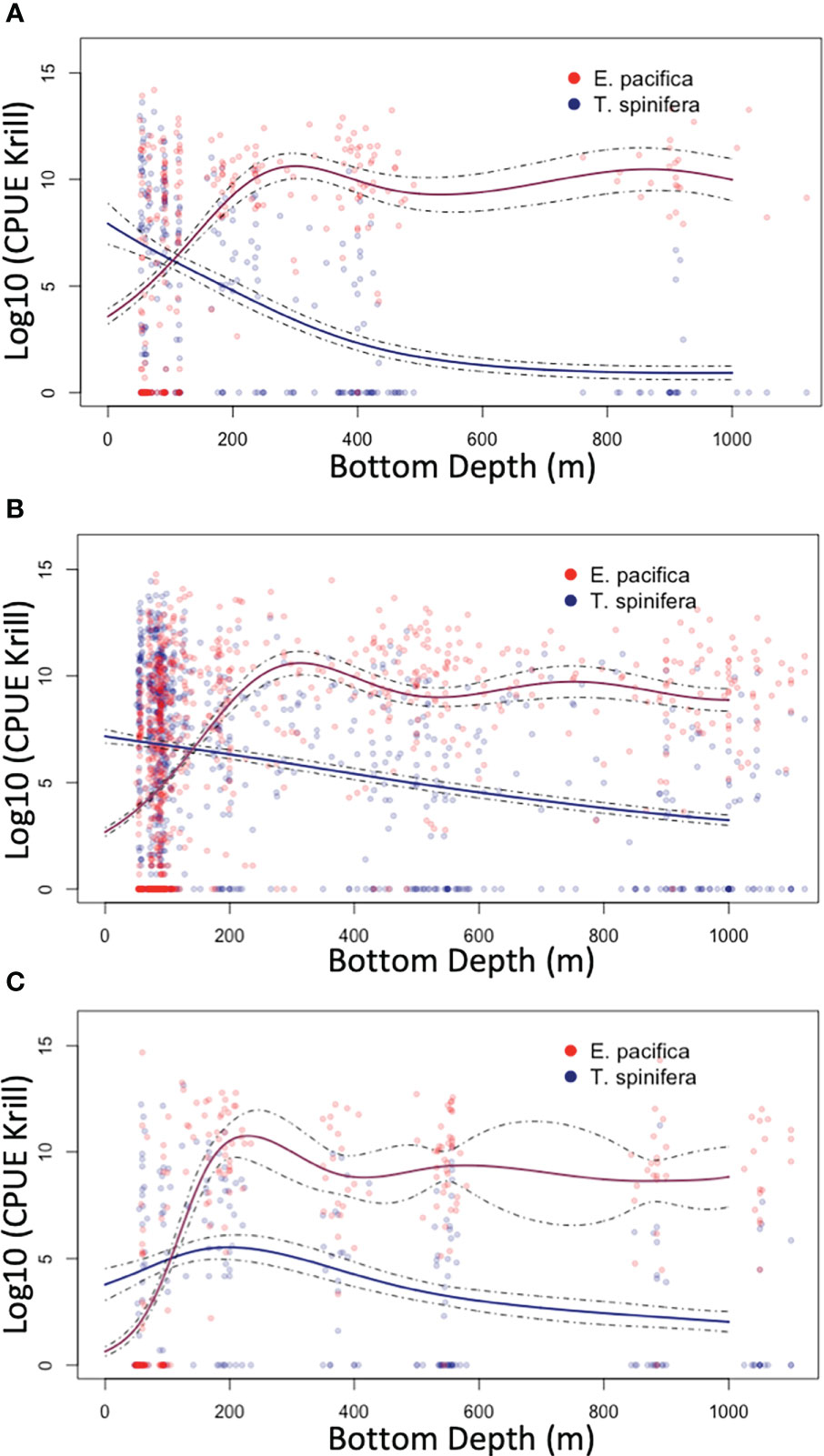
Figure 2 Generalized additive models (GAMs; derived using species-specific trawl catch per unit effort data) that were used to partition the acoustic signal into Euphausia pacifica (red) and Thysanoessa spinifera (blue) by depth: north of the core region (A), within the core region (B), and south of the core region (C).
2.2 Net data collection and processing
Krill were collected as part of micronekton sampling on the RREAS using a modified Cobb mid-water trawl with a 26-m headrope, 9.5-mm stretched mesh cod-end liner, and an optimal mouth opening of 12 m by 12 m (Sakuma et al., 2016). All trawls were done at night, for ~45 minutes duration, and with a target head-rope depth of 30 m. The trawl does not sample small krill well (<12 mm), and also likely under-samples krill 12 to 16 mm in length (Wells et al., 2012). However, the trawl samples krill >16 mm well (Cimino et al., 2020; Killeen et al., 2022) and may be better at sampling adult size classes than smaller nets (Weibe et al., 2004). Trawl nets were deployed on a regular grid as part of the larger RREAS and were not deployed specifically to sample acoustic signatures. A subsample of the total krill collected in the trawl was preserved in 10% buffered formalin and later analyzed to determine the species composition, abundance, and length-frequency of the dominant krill species in the haul. The size of the subsample (typically 200 ml, but larger when fewer krill were present) was chosen to ensure representative length frequencies of the top two to three krill species sampled by the net.
We used krill samples from mid-water trawls to model species distribution relative to bathymetry (all stations, years 2002–2018), characterize the adult population size structure (select stations, years 2012–13 and 2015–18; see Killeen et al., 2022), and calculate a krill abundance index (core stations, years 2012–2021).
2.2.1 Partitioning acoustic signal to species distribution
Three regional “climatologies” of relative abundance of E. pacifica and T. spinifera in relation to bottom depth were created using community composition data from all RREAS stations from 2002–2018 (Figure 2). Generalized additive modeling (GAM) using the R (version 4.0.0) package ‘mgcv’ (Wood, 2011, version 1.8-31, R Core Team, 2020) was used to account for non-linear relationships between log-transformed E. pacifica and T. spinifera trawl catch-per-unit effort and bathymetric depth. GAM models for each species were fit with a quasi-Poisson distribution and log-link function, and evaluated using regional cross-validations (Table S1). Regional model results were used to determine the proportion of the backscatter attributable to each species based on the bottom depth where the acoustic data were obtained.
2.2.2 Characterizing the adult population size structure
Length-frequencies of krill (Figure 3) were derived from formaldehyde-preserved sub-samples from select stations of the RREAS mid-water trawls (years 2012–2018). Data were not available from all RREAS trawl stations, but those analyzed spanned the latitudinal and onshore/offshore extent of the RREAS (Killeen et al., 2022). Krill were identified to species and sex and measured using the segmented line tool in ImageJ software (Schneider et al., 2012; Rueden et al., 2017). The station size distributions were expanded using the total krill catch from the station and annual size distributions were used to create weighting arrays (Wl) for each species (Equation 1) where nl is the number of krill sampled at each length (l), ranging from 12 mm to 35 mm in 1 mm increments. A climatology was created from the years 2012–13 and 2015–18 and applied to years with no length-frequency data (2014, 2019, 2021).
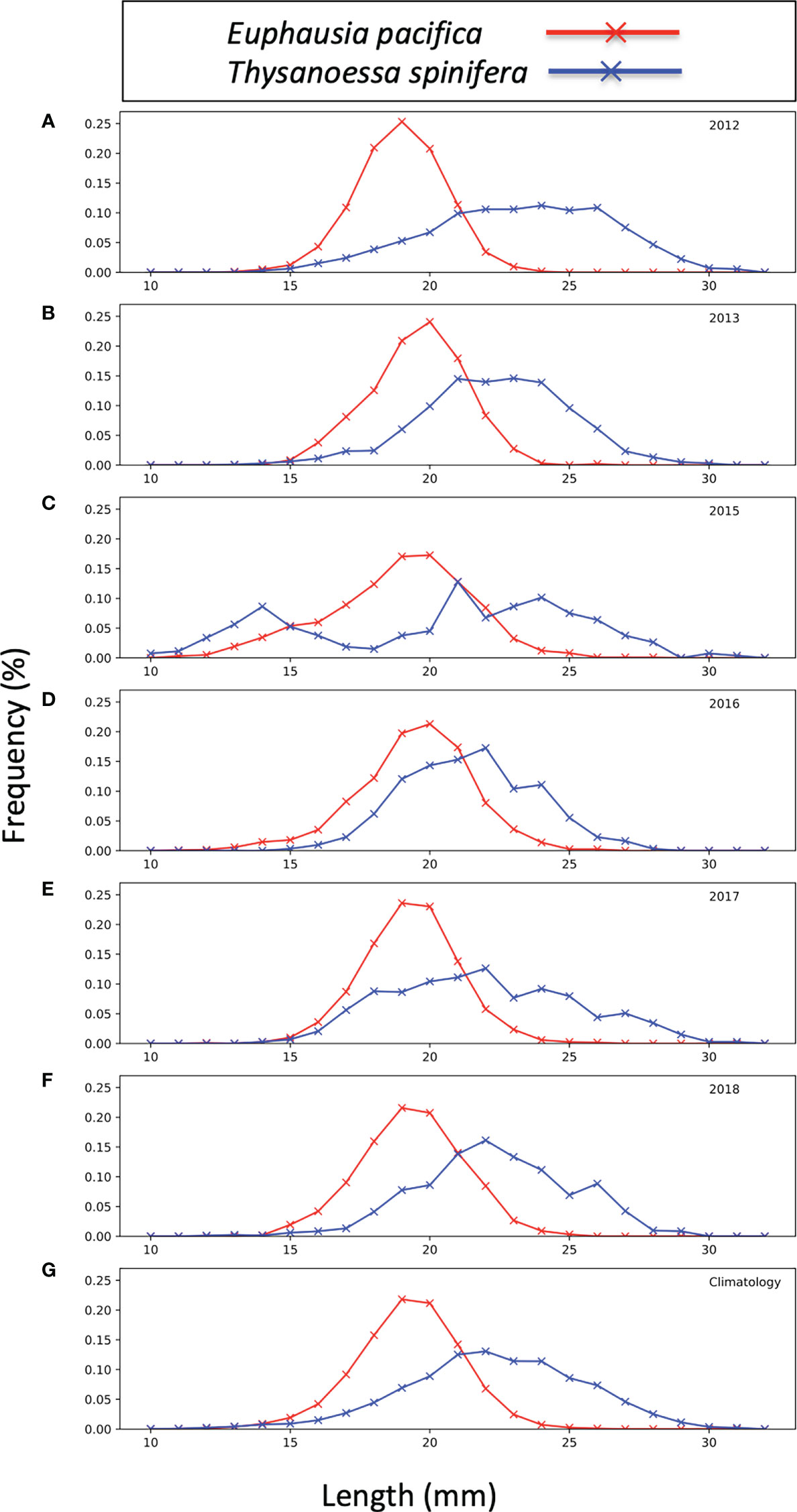
Figure 3 Euphausia pacifica (red) and Thysanoessa spinifera (blue) population size structure from 2012–13 (A, B), 2015–18 (C–F), and a combined climatology (G). Frequency is the percentage of total measured species at each length increment (mm).
Equation 1
The length-frequency data were derived from nighttime samples and our acoustic sampling was conducted during daytime (see below). We assume that we sampled the same population with the nets and acoustics as adult krill are reliable vertical migrators and do not migrate deeper than our deepest sampling depth (400 m) (Brinton, 1967; Youngbluth, 1976).
2.2.3 Krill abundance index
A relative abundance index for krill from net sampling using a delta-generalized linear model was developed and derived from Santora et al. (2021), based on the approach long used for developing groundfish recruitment indices to inform stock assessments (Ralston et al., 2013). This approach accounts for spatial and temporal sampling covariates and models presence/absence, and then abundance where present (Maunder and Punt, 2004; Ralston et al., 2013). Candidate models using varying error distributions were evaluated using the Akaike Information Criterion (AIC), and uncertainty was measured by running the model in a Bayesian framework with vague priors and computing 95% credible intervals using the package 'rstanarm' in R (Santora et al., 2021). The resulting indices, a measure of relative abundance, were log(x+1) transformed for comparative purposes with acoustic indices. Abundance indices from a suite of forage taxa estimated in this manner are reported in a collection of “ecosystem status” documents that inform fisheries managers throughout the California Current (e.g., Harvey et al., 2021; Weber et al., 2021).
2.3 Acoustic data collection and processing
Acoustic survey effort over 2012–2021 is shown in Figure 1. Acoustic survey data were collected using a Simrad EK60 (2012–2018) and a Simrad EK80 (2019–2021). The echo sounders were calibrated annually in the spring by NOAA-Southwest Fisheries Science Center before the RREAS (Stierhoff et al., 2020) and data were typically collected using a ping interval of 1 second. Data were processed using Echoview 4.9 and 12.0 (Echoview Software Pty Ltd, Hobart, Australia). Data were excluded from a) waterline to 10 m depth due to transducer depth and shipboard interference from downswept air bubbles, b) within 5 m of the bottom to avoid signal interference, and c) below 400 m in deeper waters. Visual examination of the data was conducted and data showing evidence of false bottoms, surface perturbations, obvious anomalies, and bad pings were excluded. Data collected at ship speeds below 5 nautical miles hr-1 were not processed in order to avoid periods of equipment interference and ensure unbiased comparison of the data with concurrent seabird and marine mammal surveys. Only daytime acoustic data (collected 30 minutes post-sunrise to 30 minutes prior to sunset) were included in biomass analyses because of a strong negative bias in the nighttime data due to krill migrating into surface waters above our 10-m surface depth cutoff.
Acoustic backscatter was classified as krill when the difference in volume backscatter between the 38 and 120 kHz systems, ΔSV120-38, fell within the range of previously reported values for krill (ΔSV 120-38 range = 10.9–16.7; De Robertis et al., 2010). This ΔSV range was derived from krill 16–30 mm in length, similar to the lengths of adult E. pacifica (12–25 mm) and T. spinifera (14–32 mm) in our region of study, and it has little to no overlap with measured ΔSV120-38 ranges for other species including jellies, myctophids, and other small forage fish. However, as noted by De Robertis et al. (2010), this process may not exclude scattering from other organisms such as non-euphausiid crustaceans, gelatinous zooplankton, small myctophids (which lack swim bladders) or other epipelagic micronekton. Backscatter that satisfied the ΔSV120-38 criteria for krill were used as a mask on the 120 kHz data, which were used for biomass estimates.
Volume backscattering (SV) was averaged into 0.25-nmi (horizontal) and 10-m (vertical) bins (De Robertis et al., 2010). To determine background noise, SV at all frequencies was averaged over 40 pings (horizontal) and in 10-m depth increments, and the minimum value was selected as background noise (De Robertis and Higginbottom, 2007). Data were excluded from analysis if Sv (with noise removed) was not 10 dB greater than that of the background noise.
2.4 Target strength modeling
Target strength modeling was done using the stochastic distorted-wave Born approximation (SDWBA) (Demer and Conti, 2003; Conti and Demer, 2006). Input parameters used in the target strength model were derived from measurements of krill morphology, density, and sound speed contrast from 160 individual krill (110 E. pacifica and 50 T. spinifera) collected and measured during the 2019 RREAS (Warren and Lucca, 2020). Morphology and density contrast were measured for individuals (i.e., species-specific results) whereas sound speed contrast measurements were made on groups of animals (same value for both species) due to methodological limitations (Becker and Warren, 2014; Lucca et al., 2021). The measured parameter values (Table 1) were similar in range to measurements from previous studies of euphausiids in the Northeast Pacific (Becker and Warren, 2014) and Bering Sea (Smith et al., 2010). It should be noted that the values used in this study are different than the traditional density and sound speed contrast values from Antarctic krill (i.e., Foote et al., 1990) that are commonly used for euphausiid target strength predictions.
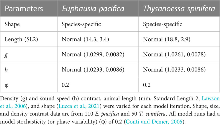
Table 1 Summary of SDWBA model inputs for each krill species with distributions (Gaussian, mean value ± standard deviation) reported where appropriate.
Mean backscattering strength of E. pacifica and T. spinifera was calculated for animals with lengths 12–35 mm in 1-mm increments. For each animal length, 1000 iterations of the model were run using normal distributions of density and sound speed contrast. Other parameters that were varied for each model iteration included animal shape (i.e., fatness as a function of animal length) based on species-specific shape measurements made during the cruise, and animal orientation with data from a previous study (Lucca et al., 2021). The modeled target strength values were then averaged (in the linear domain) to produce a mean backscattering cross-section value for each species and length increment (σBSl) that was then used for the biomass calculations.
2.5 Biomass calculations
Abundance, expressed as biomass, was estimated for E. pacifica and T. spinifera separately and together. The acoustic signal (volume backscattering – sv) was partitioned by species based on a set of regional GAMs modeling species distribution with water depth (Figure 2). Because the computation process is the same for both species, the following equations do not include denotations of species (except in Equations 5 and 6). In all equations, capital letters are used to denote arrays and lower case letters denote scalars.
Average backscattering strength of the acoustically sampled krill ( ) was calculated for each region using Equation 2.
Equation 2
Total number of krill per species per m2 (nk) was calculated as in Equation 3, and number of krill (NKl) at each length increment was calculated as in Equation 4.
Equation 3
Equation 4
Arrays of the wet weight (WW, units: mg) of E. pacifica and T. spinifera were calculated for 1-mm length (l) increments from 12 to 35 mm using Equations 5 and 6, respectively. These equations are based on a linear regression of length and weight measurements of frozen animals collected during the 2019 RREAS (see Figure 8 in Warren and Lucca, 2020) and measured in a laboratory post-cruise (E. pacifica: N = 88, R2 = 0.74; T. spinifera: N = 44, R2 = 0.81).
Equation 5
Equation 6
Finally, total species biomass (bm, units: mg m-2) was calculated as Equation 7.
Equation 7
Total krill biomass is the sum of E. pacifica and T. spinifera biomass.
2.6 Acoustic indicators of regional biomass
By averaging acoustic observations on a grid of 2,657 discrete 25-km2 cells, we developed three indicators of krill biomass: i) arithmetic mean, ii) median, and iii) geometric mean (Figure 1). This grid cell size was chosen to reduce autocorrelation between cells (Santora et al., 2011a), and to reflect a reasonable trade-off between sampling density and spatial resolution (Santora et al., 2011b). In this paper, we focus on the results derived from the arithmetic means due to the patchiness and aggregating nature of krill (see Discussion). Data coverage, the percentage of discrete grid cells sampled in at least one year within the study area, was 80.9%. The number of grid cells sampled in at least four of the nine years was 27.2%. The number of grid cells sampled in at least one year within the core region was 91.7%, and the number sampled in at least four years was 54.1%.
2.6.1 Scale-up method
We used multiple methodologies to fill grid cells that were without data. These multiple statistics and methods are presented to explore the range of outcomes in our estimates. To account for grid cells without data, the total regional biomass (bmreg) was calculated as the summed biomass across all grid cells (bmi) that contained data (ndata), converted to metric tons per grid cell (mt), and then scaled up to the entire region by dividing by the % coverage of data (Equation 8). We used this method first over all grid cells with data from the nine years, and then for only those grid cells that had at least four years of data.
Equation 8
2.6.2 Cross-shelf transect method
Mean biomass was also estimated using only data collected on cross-shelf transect lines that were consistently sampled. Cells between the adjacent lines were filled in using nearest neighbor interpolation (similar to methods in Ressler et al., 2012). Transect lines were identified by calculating the number of samples collected in small latitudinal bins (~1 km; Figure 1). Each transect line had varying degrees of sampling effort as they were not sampled in every year during daytime hours. Our preliminary analysis of transects used all identified lines (northern region n = 9, core region n = 8, southern region n = 9). A second similar analysis combined data from adjacent individual transects into eight groups based on proximity to one another (see Figure 1A).
2.6.3 Annual biomass
Annual acoustic estimates were assessed for the study area and the core region using only the scale-up method (Equation 8) because there was not enough data collected on the individual or the grouped transect lines on a year-to-year basis. Annual biomass estimates were also calculated along the four transect lines that had the most data collected on them over the nine years of the study (at 36.9°N, 37.2°N, 37.4°N, and 38.3°N; Figure 1) using the scale-up method (Equation 8; using only the discrete grid cells along the transect line). The annual gridded krill biomass was not normally distributed (Kolgomorov-Smirnov test, D = 0.29, p< 0.01) due to the presence of high-density aggregations. Thus, we used the non-parametric Kruskal-Wallis test to determine the significance of interannual variation in krill biomass.
2.6.4 Uncertainty analysis
We estimated uncertainty in biomass (due to fine-scale spatial variability within our grid cells) by running Monte-Carlo simulations (10,000 total) on the mean and standard deviation of biomass for each grid cell. Uncertainty due to variability in the parameters of the target strength model was assessed by calculating acoustic biomass using the average target strength ±1 standard deviation of . We also examined how variability in length-frequency of krill impacted biomass by comparing results calculated using an annual length-frequency to those calculated using a climatology derived from all years of data.
2.7 Krill biomass relative to environmental variation
We evaluated six measurements of krill biomass for relationships with environmental variation: total krill, E. pacifica, and T. spinifera biomass in the full study area, and total krill, E. pacifica, and T. spinifera biomass in the core study area (Figure 1). We used the Central California (34.5°N–38°N) MOCI to represent environmental conditions across years. MOCI is a seasonal index (Jan–Mar, Apr–Jun, Jul–Sep, and Oct–Dec) that integrates nine variables, including Pacific basin-scale drivers (Pacific Decadal Oscillation (PDO), ENSO) and local phenomena such as upwelling, sea surface temperature, and winds. MOCI is negative during years of cooler temperatures and stronger upwelling and positive during years of warmer temperatures and decreased upwelling. For each krill biomass variable, we examined the potential effects of winter and spring MOCI in the same year (yearx) and the four seasons from the previous year (yearx-1). Lagged relationships were examined because stanzas of warm and cool years and krill abundance have been observed (Brinton and Townsend, 2003; Santora et al., 2014), and a variety of studies have shown that winter “pre-conditioning” of the ecosystem may be a driver of population change of krill and productivity of krill predators (Black et al., 2011; Schroeder et al., 2014). To select the best model, we used forward stepwise regressions to examine relationships; MOCI variables were added sequentially at p-value < 0.1 starting with the one that was most highly related to krill biomass. Additional variables were added sequentially if they were significantly related to krill biomass after the inclusion of variables entered earlier in the stepwise process.
3 Results
3.1 Mean regional biomass (2012–2021)
Krill biomass for California ranged from 1,715 to 1,974 thousand metric tons (kmt) (Table 2; Figure 4). The 95% confidence intervals of the results using the scale-up method were ±204 mt when using all data, and ±443 mt when using only those grid cells with four or more years of data.
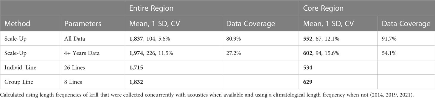
Table 2 2012–2021 Mean krill biomass (thousands of metric tons (kmt); bold), standard deviation (SD, kmt), coefficient of variation (CV), and percent data coverage of the region.
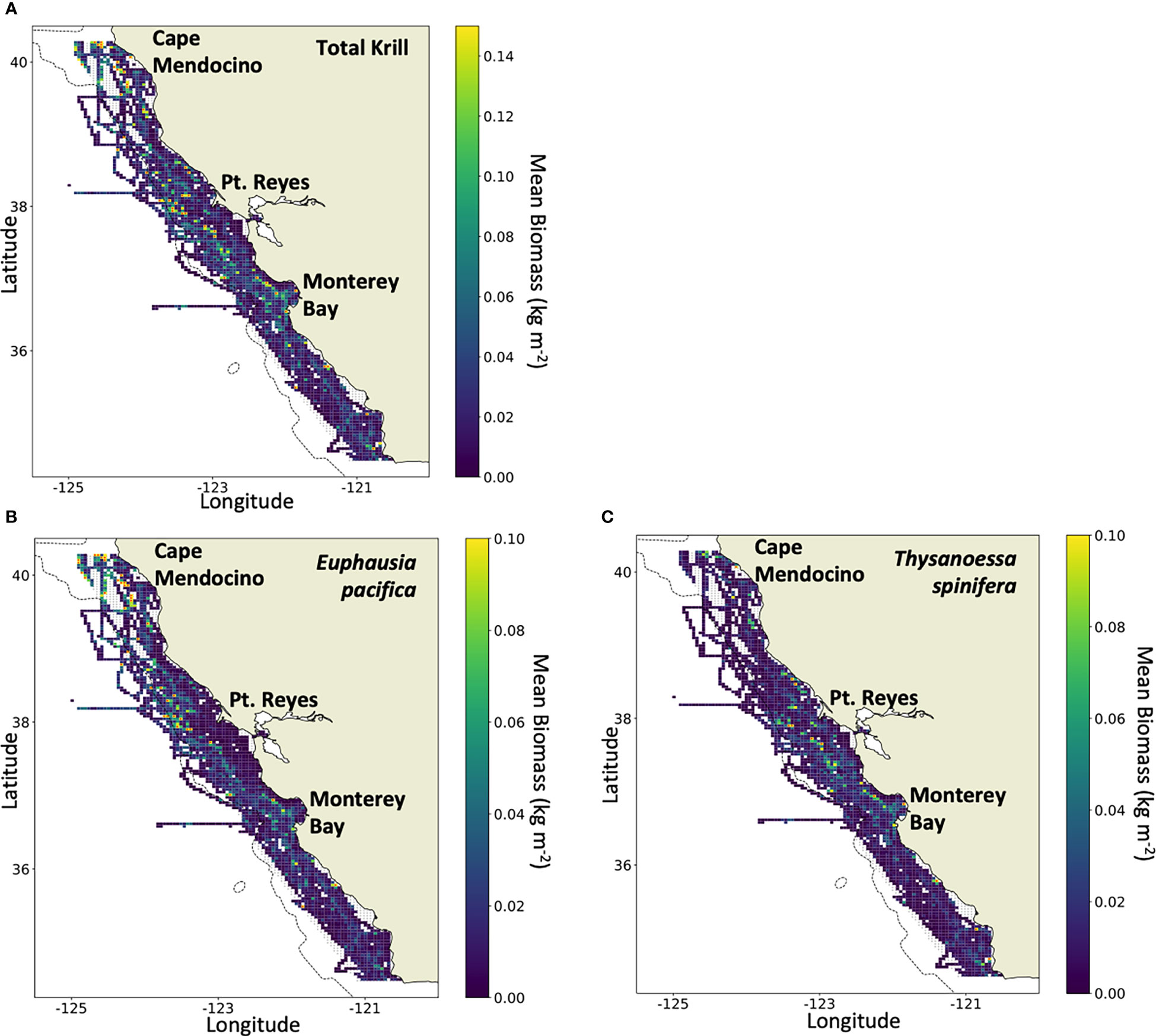
Figure 4 Mean biomass density (kg m-2) in the study area, 2012–2021, of (A) total krill, (B) Euphausia pacifica, and (C) Thysanoessa spinifera (note the varying difference in scales). Grid cells with a red marker exceed the maximum biomass set by the color scale. Maximum biomass density was (A) 0.60 kg m-2 of total krill, (B) 0.51 kg m-2 of E pacifica, and (C) and 0.22 kg m-2 of T. spinifera.
Krill biomass for the core sampling region ranged from 534 to 629 kmt (Table 2). The 95% confidence intervals of the results using the scale-up method were ±131 mt when using all data and ±184 mt when using only those grid cells with four or more years of data.
Biomass estimates derived from the median and geometric mean are presented in supplemental material (Table S2). These indices of abundance were different from arithmetic mean abundance, but for reasons detailed below (Discussion) we focus on the results of arithmetic means.
3.2 Interannual variation in biomass
Biomass ranged from a low of 1,162 kmt in 2016 to a high of 2,494 kmt in 2018 (Table 3), with 95% confidence intervals of ±9.4% and ±33.9%. Overall, E. pacifica was slightly more abundant each year (≥50.8% of the biomass), except in 2012 when T. spinifera was more abundant (56.4% of the biomass; Table 3). However, within the core region, T. spinifera was consistently more abundant (≥54.5%; Table 4). In this region, interannual variation in biomass ranged from 367 kmt in 2016 to 851 kmt in 2018 (Table 4; Figure S1), with 95% confidence intervals of ±15.5% to ±73.9%, respectively. Estimated annual total krill biomass was significantly lower in 2015–2016 than in other years (H = 192.2, p< 0.0001; Table 4; Figure S1).
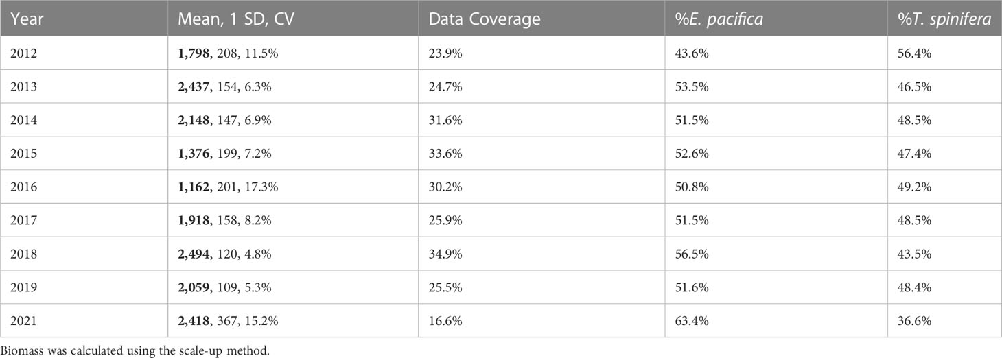
Table 3 Annual krill biomass (thousands of metric tons (kmt); bold), standard deviation (SD, kmt), coefficient of variation (CV), percent data coverage, and percent biomass of each species from the entire region.
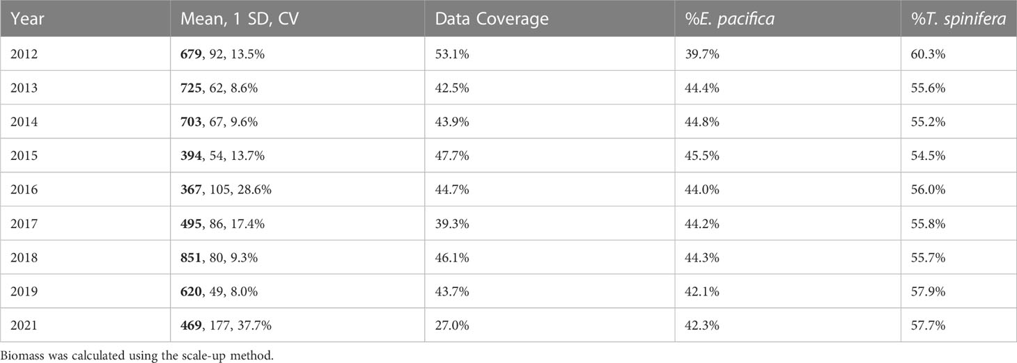
Table 4 Annual krill biomass (thousands of metric tons (kmt); bold), standard deviation (SD, kmt), coefficient of variation (CV), percent data coverage, and percent biomass of each species from the core region.
Interannual variation in acoustically-derived biomass in the core region was positively, but not significantly, related to krill relative abundance from net samples (R2 = 0.20, p = 0.23, n = 9; Figure 5). Prior to 2019, the relationship between the acoustic and net samples was even stronger (R2 = 0.65, p< 0.05, n = 7).
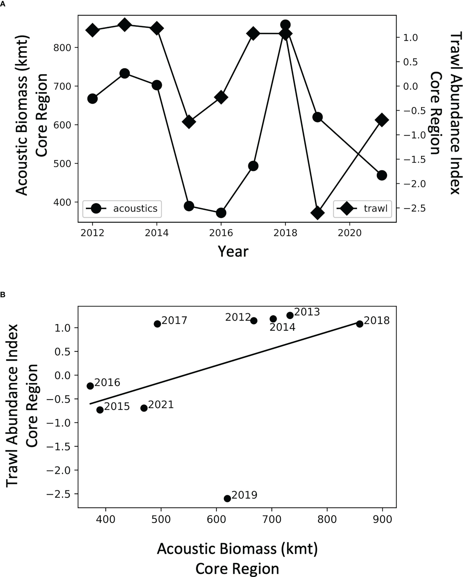
Figure 5 (A) Time series of acoustic biomass of krill (•) and a krill abundance index (♦) determined from trawl nets in the core area, and (B) regression of same data.
3.3 Relationship between krill biomass and ocean climate
Five of the six krill biomass variables were related to seasonal MOCI in a negative fashion, i.e., krill biomass decreased with increasing values of MOCI (Table 5). T. spinifera and total krill biomass in the full study area were correlated with summer MOCI in the previous year, while all three biomass variables from the core region were predicted by spring MOCI in the previous year (Table 5). In each of these relationships, 2018 appears to be a potential outlier (Figure 6). Models explained 39% to 76% of the variation in krill biomass between years.
Table 5 Results of forward stepwise regression of krill biomass in the full and core regions predicted by seasonal MOCI.
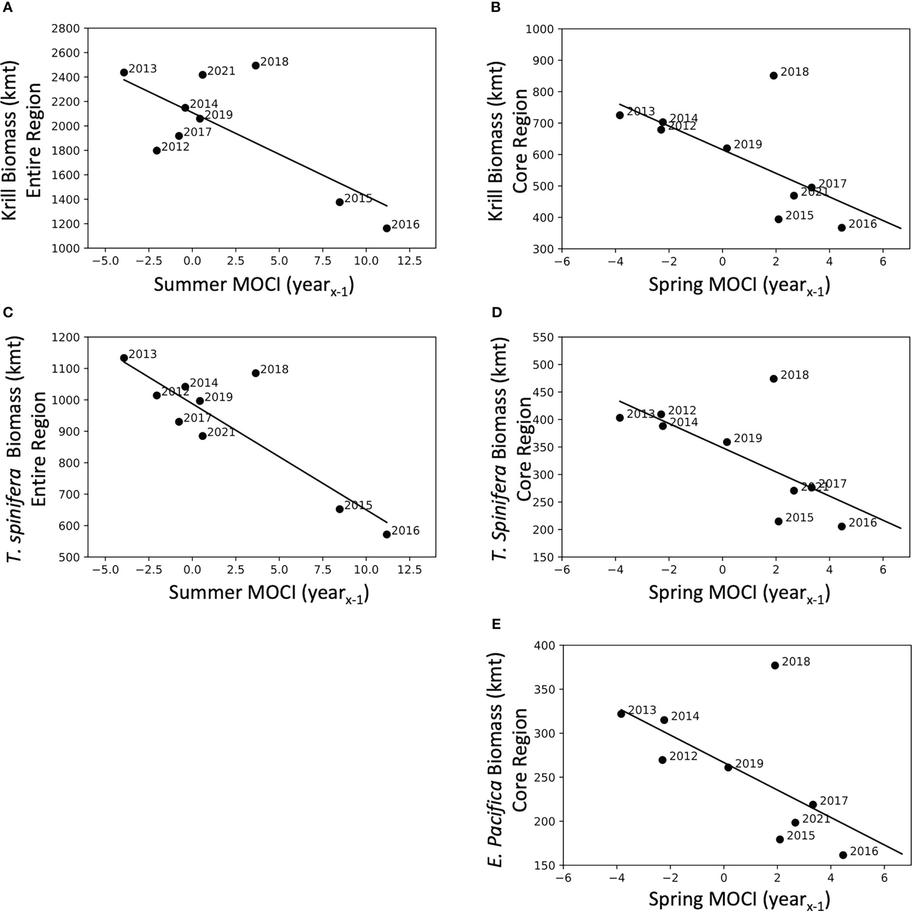
Figure 6 Krill biomass predicted by seasonal MOCI in the previous year (yearx-1). Krill biomass (A) and Thysanoessa spinifera biomass (C) for the entire region compared to Summer MOCI (yearx-1), and krill biomass (B), T. spinifera biomass (D), and Euphausia pacifica biomass (E) from the core region compared to Spring MOCI (yearx-1). Coefficients of determination and significance are reported in Table 5.
4 Discussion
Our study quantified long-term interannual variability of krill species biomass through an integration of acoustic and mid-water trawl surveys, species distribution modeling, and assessment of ocean-climate variability. There are several important conclusions informed by our study, most of which support previous research on variability of krill abundance within the central California Current. First, we estimated krill biomass during a decade of substantial environmental variability. Observations were collected during years of both weak and strong upwelling and notable warming events, suggesting they represent what may be considered the range of interannual variation in krill species biomass in this region. We estimate the average adult krill biomass in the study area and core region to be 1,750 to 2,000 kmt (26.3–30.1 mt km-2) and 550 to 650 kmt (31.0–36.0 mt km-2), respectively. Second, we found that ocean-climate conditions, inferred by a multivariate indicator, relate to krill biomass at the time of sampling and the year prior, highlighting that krill populations respond to several years of cooler ocean temperatures and upwelling conditions. Although this supports previous research (Santora et al., 2014; Cimino et al., 2020; Fiechter et al., 2020), this finding is important because multivariate indicators may better integrate scales of space-time variability than univariate comparisons alone, and benefit communicating potential changes in krill biomass a year ahead to improve timeliness of ecosystem assessments. However, on the use of multivariate indicators, we acknowledge that this approach does not infer actual mechanisms that govern interannual variation in krill biomass, but does provide a novel approach for developing integrated ecosystem monitoring. Third, our krill species biomass estimates have implications for ecosystem modeling and advancing survey methodologies. We discuss each of these points in subsequent sections below and provide recommendations and address potential uncertainties needing to be resolved with future research.
4.1 Interannual variation in biomass
Annual adult krill biomass estimates for the region varied widely over the 10-year period with the greatest/least biomass values ~600 kmt above/below the 2012–2021 average (±~30%). The core region exhibited similar variability (±~200 kmt, 30% of the mean value). The two years of lowest krill biomass, 2015 and 2016, coincided with a period of intense warming in the North Pacific from mid 2014 through 2016 (Bond et al., 2015; Gentemann et al., 2017). Warm water temperatures persisted in the nearshore environment throughout most of 2015 and into 2016 as strong El Niño conditions developed during this period (Di Lorenzo and Mantua, 2016). Reduced productivity in the California Current coastal ecosystem is generally associated with warm ocean conditions, particularly El Niño events (Lenarz et al., 1995; Marinovic et al., 2002). As a consequence, decreased krill biomass is expected given ecosystem dynamics during this warm water period (see also Brinton and Townsend, 2003; Santora et al., 2020). A similar marine heatwave occurred in summer 2019, but after the RREAS sampling had concluded. In contrast, we also note the high krill biomass in 2013 and 2018. Record-breaking upwelling intensity in April–June 2013 (Thompson et al., 2019) promoted increased productivity in the system that is reflected in the high krill biomass that year. Indicators of ecosystem productivity (e.g., MOCI) also suggested highly favorable conditions for biological productivity in 2013 and 2018. Acoustic surveys of krill over a similar set of years (from later in the summer) also found 2013 to be a year of high krill abundance and 2015 to be a year of very low abundance (Phillips et al., 2022).
Despite the interannual variability in adult krill biomass, the percentage of krill that our models partitioned to E. pacifica and T. spinifera remained remarkably consistent over the study period. Because our species partitioning model is a function of depth, this reflects the consistency of the cross-shelf location of the acoustic signal between years. Our results are also consistent with previous studies that found the most krill biomass along the shelf break and near submarine canyons (Santora et al., 2011a; Santora et al., 2018). Future species partitioning schemes could incorporate more factors beyond depth, and may provide more variability in species composition (Cimino et al., 2020). Certainly, better species-specific biomass information is important as E. pacifica is ubiquitous in the North Pacific and supports many predators, while the larger T. spinifera is more limited in range but is more energetically valuable (Fisher et al., 2020), and is a preferred prey for some specialist predators including seabirds (Abraham and Sydeman, 2006) and cetaceans (Nickels et al., 2019).
Annual variation in acoustic krill biomass in relation to the previous year’s environmental conditions, as measured by MOCI, could reflect the impact of prior year conditions on fecundity, recruitment, and ultimately survival to the next year. Krill reproduction happens throughout most of the year (Feinberg and Peterson, 2003; Feinberg et al., 2010), but there is a seasonal peak in reproduction during the period of strongest upwelling each year (Feinberg et al., 2010). The more neritic species, T. spinifera, is thought to be more responsive to the timing and intensity of upwelling than E. pacifica (Schroeder et al., 2014), and in this regard it is of note that the correlations with MOCI were marginally stronger with T. spinifera than E. pacifica. The density of eggs in the water also is positively related to chlorophyll a (Feinberg et al., 2010), thus a more productive upwelling season likely leads to more eggs and larvae produced. Development time from egg to juvenile is approximately 2 months (Ross, 1981; Feinberg et al., 2006), and to a reproductive adult is 5–8 months, though this is temperature dependent (Ross, 1982). Thus, the adult krill that are sampled during our surveys in May/June each year are undoubtedly spawned in the previous year.
We note, however, that more eggs in the water does not necessarily translate to greater number of surviving adults in the next year, but favorable environmental conditions in the seasons following spawning can lead to larger krill (Robertson and Bjorkstedt, 2020). Krill also have the ability to shrink in response to poor food conditions (Marinovic and Mangel, 1999; Shaw et al., 2010; Shaw et al., 2021), thus conveying a survival advantage to larger krill as they can withstand poor food conditions for longer periods of time. Other factors such as predation and transport could also influence survival and local abundance, but are beyond the scope of this study.
Last, the lagged correlations between krill biomass and environmental variation corroborates a recent previous study showing relationships between water temperature, krill abundance, and the timing of blue whale arrival in the Southern California Bight (Szesciorka et al., 2020). In that study, cooler waters, presumably reflecting upwelling and primary production in a previous year, also led to higher krill biomass and earlier whale arrival time off Southern California.
4.2 Implications for ecosystem modeling
Our estimates of adult krill biomass are generally higher than estimates developed from mass-balance ecosystem models and those from more localized studies using net samples (Table 6). This is perhaps due to the finer-scale sampling provided by acoustic surveys and the ability to consistently sample small-scale dense swarms of krill. More than 50% of the acoustic biomass we measured came from less than 7% of our acoustic samples (Table 7), highlighting the importance of fine-scale sampling when attempting to estimate biomass of swarming zooplankton and the location of high-density aggregations. Models with limited spatial components (ECOPATH and Atlantis) are not designed to capture this fine-scale spatial variability, but should be capable of fitting or matching such variability in response to physical forcing to provide realistic evaluations of ecosystem dynamics. Similarly, while both fine-mesh midwater trawl and bongo nets sample at small spatial scales, they typically cannot be deployed in large enough numbers to provide continuous distribution information. Acoustic sampling of krill achieves this small-scale resolution while also collecting an extensive spatial scale of data in a small amount of time. These acoustic survey data clearly indicate that all three regions of the study area support substantial krill biomass that exhibits considerable interannual variability, likely in response to oceanographic conditions. Previous ecosystem modeling studies utilized acoustic survey data for evaluating model performance for predicting interannual variation and intensity of krill hotspots (Santora et al., 2013; Fiechter et al., 2020; Messié et al., 2022). However, at the time of those studies, krill biomass estimates were unavailable, so model evaluations were made based on relative comparisons of hotspot location from observations and models. Therefore, the krill biomass estimates developed in this study provide an important step for informing krill biomass modeling study design, addressing sensitivities to environmental variability, and providing reference points for comparison with existing models. Future effort should focus on developing krill species biomass distribution models to complement existing models of species occurrence and abundance inferred by trawls (Cimino et al., 2020; Fiechter et al., 2020).
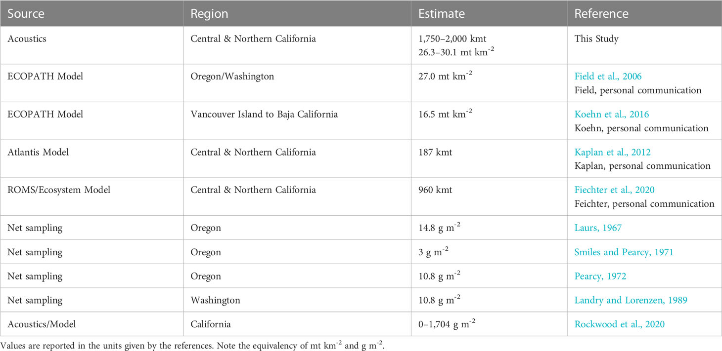
Table 6 Comparison of reported krill biomass estimates from modeling and net sampling studies along the West Coast of the United States.
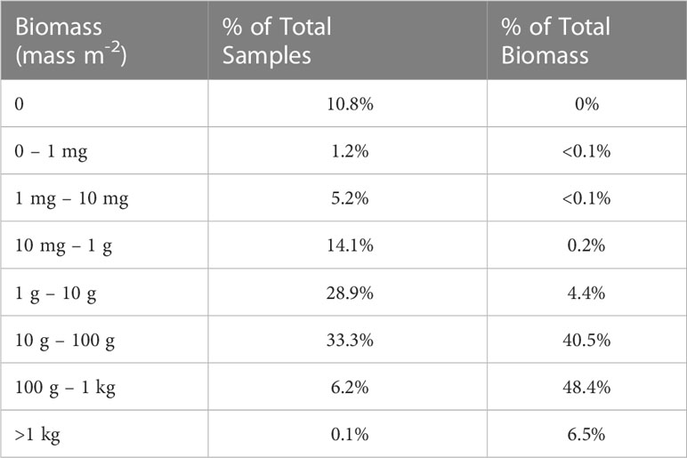
Table 7 Breakdown of acoustic samples (n = 83,478) by order of magnitude biomass bins and their contribution to the total biomass measured.
These could ultimately be used to compare krill-predator distribution patterns to better understand species consumption patterns and bioenergetic needs (Szesciorka et al., 2022).
4.3 Implications for ecosystem monitoring
Annual estimates of krill derived from hydroacoustics were positively associated with a relative krill index of abundance from trawl nets. This correspondence, shown for the region of the most robust sampling, suggests that acoustic data for the larger survey region provide robust samples as well. There were notable years in which the relationship between net data and acoustic data broke down (2019, in particular). Net hauls in 2019 brought in very little krill, but a biomass of 620 kmt of krill in the core region was estimated from acoustics. This could be due to the different sampling frequency of the two methods, as the acoustic data are collected while ships are underway and therefore are based on considerably greater spatial data than the sampling by nets which are made on station points. In short, we are uncertain about this discrepancy, which warrants further investigation of sampling, processing, and analytical details of 2019. One could, for example, examine the cross-shelf transects for consistency in sampling, and then investigate the covariance in regional indices from nets and acoustics; these detailed analyses are beyond the scope of this paper.
The various calculations of krill biomass we present show a range of estimates. We highlighted results derived from the arithmetic mean of the raw data because this procedure does not discount the important contributions of extremely large aggregations to overall abundance. Both the median and geometric mean calculations lessen the contributions of large aggregations to estimates of krill abundance; median and geometric mean-based estimates may be biased low. California Current krill are known to aggregate on both the small scale of swarms (10s–100s of meters; Mauchline, 1980; Siegel, 2000) as well as larger scales (10s–100s of kilometers) along topographical features such as canyons and the shelf break (Santora et al., 2011a; Dorman et al., 2015; Santora et al., 2018). The high-resolution hydroacoustic sampling used in this study (binned at 0.25-nmi horizontal by 10-m depth intervals) can resolve fine-scale krill aggregations, but a statistical bias of this sampling is a highly-skewed distribution of the raw data, due to many low and a few large values (see Table 7 ). Indeed, the smallest 60% of our samples accounted for <5% of the total biomass and the largest 6% accounted for >50% of the total. The skewed distribution of krill abundance data and the importance of patchy, dense aggregations must be taken into consideration in developing realistic estimates of abundance. This is accomplished using the arithmetic mean of the raw data.
The majority of the results and discussion on uncertainty of estimates is contained within Supplemental Material, but we highlight here how variability in the length-frequency data used in the calculations impacts biomass estimates. Length data are not always available, and in this study, we lacked length data in three years (2014, 2019, and 2021). For these years we used the average length frequency distributions based on the other seven years of sampling. In comparing biomass estimates using length-frequencies from specific years versus using the climatological length-frequency, we find very little effects on biomass (<3%; Table 3 vs. Table S3, Table 4 vs. Table S4).
5 Conclusions
Acoustic-trawl surveys of krill in the California Current give us a starting point from which we can better assess interannual variability in prey fields and its potential effect on upper trophic level consumers of economic and conservation importance. The interannual variability in biomass was considerable, lowest during the 2015–2016 marine heat wave/ENSO event and highest when upwelling was strongest. Krill biomass was related to physical conditions (MOCI) in the prior year’s spring and summer, suggesting that growth to enable overwintering of krill may be an important driver of krill abundance. These data suggest a direct connection to upper trophic level productivity since fish, birds, and mammals all show similar variability to the ecosystem changes in these years. As krill are a vital ecosystem component, empirically derived abundance estimates are critical for future ecosystem modeling to resolve key management and conservation questions in the California Current system.
Data availability statement
The datasets presented in this study can be found in online repositories. The names of the repository/repositories and accession number(s) can be found in the article/Supplementary Material.
Author contributions
JD & WS contributed to conception and design of the research, data analysis and interpretation, and drafting and revising content. SAT, HK & BH contributed to data analysis and revising content. JW contributed to data acquisition, analysis and interpretation, and drafting and revising content. JF & JS contributed to data collection and interpretation, and drafting and revising content. All authors contributed to the article and approved the submitted version.
Funding
This work was supported by the California Sea Grant College Program Project through NOAA’s National Sea Grant College Program, U.S. Dept. of Commerce [Sea Grant number R/SFA-03; NOAA number #NA18OAR4170073], and also by the Marisla Foundation (from 2017–2021). The statements, findings, conclusions and recommendations are those of the author(s) and do not necessarily reflect the views of California Sea Grant, NOAA or the U.S. Dept. of Commerce.
Acknowledgments
We would like to thank the scientists who collected data during the NOAA-NMFS Rockfish Recruitment Ecosystem Assessment Surveys, in particular Keith Sakuma, who was the Chief Scientist for this survey from 2012–2021. We also thank Dr. Sandra Parker-Stetter and Dr. Elizabeth Phillips for their expertise and guidance to ensure our acoustic processing was done using the best available methodology. We also thank Dr. Baldo Marinovic for sharing his data on the length-frequency distribution of krill from these same cruises, and Ilysa Iglesias for her thoughtful comments and suggestions on an earlier draft of this manuscript.
Conflict of interest
The authors declare that the research was conducted in the absence of any commercial or financial relationships that could be construed as a potential conflict of interest.
Publisher’s note
All claims expressed in this article are solely those of the authors and do not necessarily represent those of their affiliated organizations, or those of the publisher, the editors and the reviewers. Any product that may be evaluated in this article, or claim that may be made by its manufacturer, is not guaranteed or endorsed by the publisher.
Supplementary material
The Supplementary Material for this article can be found online at: https://www.frontiersin.org/articles/10.3389/fmars.2023.1099482/full#supplementary-material
References
Abraham C. L., Sydeman W. J. (2006). Prey-switching by cassin's auklet Ptychoramphus aleuticus reveals seasonal climate-related cycles of Euphausia pacifica and Thysanoessa spinifera. Mar. Ecol. Prog. Ser. 313, 271–283. doi: 10.3354/meps313271
Atkinson A., Siegel V., Pakhomov E. A., Jessopp M. J., Loeb V. (2009). A re-appraisal of the total biomass and annual production of Antarctic krill. Deep-Sea Res. Pt. I 56, 727–740. doi: 10.1016/j.dsr.2008.12.007
Aydin K., Mueter F. (2007). The Bering Sea–a dynamic food web perspective. Deep-Sea Res. Pt. II 54, 2501–2525. doi: 10.1016/j.dsr2.2007.08.022
Becker K. N., Warren J. D. (2014). Material properties of northeast pacific zooplankton. ICES J. Mar. Sci. 71, 2550–2563. doi: 10.1093/icesjms/fsu109
Black B. A., Schroeder I. D., Sydeman W. J., Bograd S. J., Wells B. K., Schwing F. B. (2011). Winter and summer upwelling modes and their biological importance in the California current ecosystem. Glob. Change Biol. 17, 2536–2545. doi: 10.1111/j.1365-2486.2011.02422.x
Bond N. A., Cronin M. F., Freeland H., Mantua N. (2015). Causes and impacts of the 2014 warm anomaly in the NE pacific. Geophys. Res. Lett. 42, 3414–3420. doi: 10.1002/2015GL063306
Brierley A. S., Watkins J. L., Murray A. W. A. (1997). Interannual variability in krill abundance at south Georgia. Mar. Ecol. Prog. Ser. 150, 87–98. doi: 10.3354/meps150087
Brinton E. (1962). The distribution of pacific euphausiids. Bull. Scripps Inst. Oceanogr. 8, 51–269.
Brinton E. (1967). Vertical migration and avoidance capability of euphausiids in the California current. Limnol. Oceanogr. 12, 451–481. doi: 10.4319/lo.1967.12.3.0451
Brinton E., Townsend A. (2003). Decadal variability in abundances of the dominant euphausiid species in southern sectors of the California current. Deep-Sea Res. Pt. II 50, 2449–2472. doi: 10.1016/S0967-0645(03)00126-7
Cavan E. L., Belcher A., Atkinson A., Hill S. L., Kawaguchi S., McCormack S., et al. (2019). The importance of Antarctic krill in biogeochemical cycles. Nat. Commun. 10, 4742. doi: 10.1038/s41467-019-12668-7
Checkley D. M., Barth J. A. (2009). Patterns and processes in the California current system. Prog. Oceanogr. 83, 49–64. doi: 10.1016/j.pocean.2009.07.028
Christensen V., Pauly D. (1992). ECOPATH II – a software for balancing steady-state ecosystem models and calculating network characteristics. Ecol. Mod. 61, 169–185. doi: 10.1016/0304-3800(92)90016-8
Christensen V., Walters C. J. (2004). Ecopath with ecosim: Methods, capabilities and limitations. Ecol. Mod. 172, 109–139. doi: 10.1016/j.ecolmodel.2003.09.003
Cimino M. A., Santora J. A., Schroeder I., Sydeman W., Jacox M. G., Hazen E. L., et al. (2020). Essential krill species habitat resolved by seasonal upwelling and ocean circulation models within the large marine ecosystem of the California current system. Ecography 43, 1536–1549. doi: 10.1111/ecog.05204
Conti S. G., Demer D. A. (2006). Improved parameterization of the SDWBA for estimating krill target strength. ICES J. Mar. Sci. 63, 928–935. doi: 10.1016/j.icesjms.2006.02.007
Coyle K. O., Pinchuk A. I. (2002). The abundance and distribution of euphausiids and zero-age pollock on the inner shelf of the southeast Bering Sea near the inner front in 1997–1999. deep-Sea res. Pt. II 49, 6009–6030. doi: 10.1016/S0967-0645(02)00331-4
Croll D. A., Marinovic B., Benson S., Chavez F. P., Black N., Ternullo R., et al. (2005). From wind to whales: Trophic links in a coastal upwelling system. Mar. Ecol. Prog. Ser. 289, 117–130. doi: 10.3354/meps289117
Demer D. A., Conti S. G. (2003). Reconciling theoretical versus empirical target strengths of krill: Effects of phase variability on the distorted-wave born approximation. ICES J. Mar. Sci. 60, 429–434. doi: 10.1016/S1054-3139(03)00002-X
De Robertis A., Higginbottom I. (2007). A post-processing technique to estimate the signal-to-noise ratio and remove echosounder background noise. ICES J. Mar. Sci. 64, 1282–1291. doi: 10.1093/icesjms/fsm112
De Robertis A., McKelvey D. R., Ressler P. H. (2010). Development and application of an empirical multifrequency method for backscatter classification. Can. J. Fish. Aquat. Sci. 67, 1459–1474. doi: 10.1139/F10-075
Di Lorenzo E., Mantua N. (2016). Multi-year persistence of the 2014/15 north pacific marine heatwave. Nat. Clim. Change 6, 1042–1048. doi: 10.1038/nclimate3082
Dorman J. G., Bollens S. M., Slaughter A. M. (2005). Population biology of euphausiids off northern California and effects of short time-scale wind events on Euphausia pacifica. Mar. Ecol. Prog. Ser. 288, 183–198. doi: 10.3354/meps288183
Dorman J. G., Powell T. M., Sydeman W. J., Bograd S. J. (2011). Advection and starvation cause krill (Euphausia pacifica) decreases in 2005 northern California coastal populations: Implications from a model study. Geophys. Res. Lett. 38, L04605. doi: 10.1029/2010GL046245
Dorman J. G., Sydeman W. J., García-Reyes M., Zeno R. A., Santora J. A. (2015). Modeling krill aggregations in the central-northern California current. Mar. Ecol. Prog. Ser. 528, 87–99. doi: 10.3354/meps11253
Dufault A. M., Marshall K., Kaplan I. C. (2009). A synthesis of diets and trophic overlap of marine species in the California current. NOAA Tech. Memorandum NMFS-NWFSC 103, 81.
Eriksen E., Dalpadado P. (2011). Long-term changes in krill biomass and distribution in the barents Sea: Are the changes mainly related to capelin stock size and temperature conditions? Polar Biol. 34, 1399–1409. doi: 10.1007/s00300-011-0995-0
Evans R., English P. A., Anderson S. C., Gauthier S., Robinson C. L. (2021). Factors affecting the seasonal distribution and biomass of e. pacifica and T. spinifera along the pacific coast of Canada: A spatiotemporal modelling approach. PloS One 16 (5), 0249818. doi: 10.1371/journal.pone.0249818
Feinberg L. R., Peterson W. T. (2003). Variability in duration and intensity of euphausiid spawning off central Oregon 1996–2001. Prog. Oceanogr. 57, 363–379. doi: 10.1016/S0079-6611(03)00106-X
Feinberg L. R., Peterson W. T., Shaw C. T. (2010). The timing and location of spawning for the euphausiid Thysanoessa spinifera off the Oregon coast, USA. Deep-Sea Res. Pt. II 57, 572–583. doi: 10.1016/j.dsr2.2009.10.007
Feinberg L. R., Shaw C. T., Peterson W. T. (2006). Larval development of Euphausia pacifica in the laboratory: Variability in developmental pathways. Mar. Ecol. Prog. Ser. 316, 127–137. doi: 10.3354/meps316127
Fiechter J., Santora J. A., Chavez F., Northcott D., Messie M. (2020). Krill hotspot formation and phenology in the California current ecosystem. Geophys. Res. Lett. 47, e2020GL088039. doi: 10.1029/2020GL088039
Field J. C., Francis R. C., Aydin K. (2006). Top-down modeling and bottom-up dynamics: Linking a fisheries-based ecosystem model with climate hypotheses in the northern California current. Prog. Oceanogr. 68, 238–270. doi: 10.1016/j.pocean.2006.02.010
Fisher J. L., Menkel J., Copeman L., Shaw C. T., Feinberg L. R., Peterson W. T. (2020). Comparison of condition metrics and lipid content between Euphausia pacifica and Thysanoessa spinifera in the northern California current, USA. Prog. Oceanogr. 188, 102417. doi: 10.1016/j.pocean.2020.102417
Foote K. G., Everson I., Watkins J. L., Bone D. G. (1990). Target strengths of Antarctic krill (Euphausia superba) at 38 and 120 kHz. J. Acoust. Soc Amer. 87, 16–24. doi: 10.1121/1.399282
García-Reyes M., Sydeman W. J. (2017). California Multivariate ocean climate indicators (MOCI) and marine ecosystem dynamics. Ecol. Ind. 72, 521–529. doi: 10.1016/j.ecolind.2016.08.045
Gentemann C. L., Fewings M. R., García-Reyes M. (2017). Satellite sea surface temperatures along the West coast of the united states during the 2014–2016 northeast pacific marine heat wave. Geophys. Res. Lett. 44, 312–319. doi: 10.1002/2016GL071039
Harvey C. J., Garfield N., Williams G. D., Tolimieri N., (Eds.) (2021). Ecosystem status report of the California current for 2020–21: A summary of ecosystem indicators compiled by the California current integrated ecosystem assessment team (CCIEA) (U.S. Department of Commerce, NOAA Technical Memorandum NMFS-NWFSC-170). doi: 10.25923/x4ge-hn11
Kaplan I. C., Horne P. J., Levin P. S. (2012). Screening California Current fishery management scenarios using the Atlantis end-to-end ecosystem model. Progress in Oceanography 102, 5–18. doi: 10.1016/j.pocean.2012.03.009
Killeen H., Dorman J. D., Sydeman W., Dibble C., Morgan S. (2022). Effects of a marine heatwave on adult body length of three numerically dominant krill species in the California current ecosystem. ICES J. Mar. Sci. 79, 761–774. doi: 10.1093/icesjms/fsab215
Koehn L. E., Essington T. E., Marshall K. N., Kaplan I. C., Sydeman W. J., Szoboszlai A. I., et al. (2016). Developing a high taxonomic resolution food web model to assess the functional role of forage fish in the California Current ecosystem. Ecological Modelling 335, 87–100. doi: 10.1016/j.ecolmodel.2016.05.010
Landry M. R., Lorenzen C. J. (1989). Abundance, distribution and grazing impact of zo-oplankton on the Washington shelf. In Landry M. R., Hickey B. M. (editors) Coastal Oceanography of Washington and Oregon. Elsevier: Amsterdam.
Laurs R. M. (1967). Coastal upwelling and ecology of lower trophic levels. Ph.D. Dissertation. Oregon State University.
Lawson G. L., Wiebe P. H., Ashjian C. J., Chu D., Stanton T. K. (2006). Improved parametrization of Antarctic krill target strength models. The Journal of the Acoustical Society of America 119(1), 232–242.
Leising A. W., Schroeder I. D., Bograd S. J., Bjorksted E., Field J., Sakuma K., et al. (2014). State of the California current 2013–2014: El nino looming. Cal. Coop. Oceanic Fish. Invest. Rep. 55, 51–87.
Lenarz W. H., Ventresca D. A., Graham W. M., Schwing F. B., Chavez F. (1995). Explorations of El niño events and associated biological population dynamics off central California. Cal. Coop. Oceanic Fish. Invest. Rep. 36, 106–119.
Lilly L. E., Ohman M. D. (2021). Euphausiid spatial displacements and habitat shifts in the southern California current system in response to El niño variability. Prog. Oceanogr. 193, 102544. doi: 10.1016/j.pocean.2021.102544
Lucca B. M., Ressler P. H., Harvey H. R., Warren J. D. (2021). Individual variability in sub-Arctic krill material properties, lipid composition, and other scattering model inputs affect acoustic estimates of their population. ICES J. Mar. Sci. 78, 1470–1484. doi: 10.1093/icesjms/fsab045
Marinovic B., Croll D. A., Gong N., Benson S. R., Chavez F. P. (2002). Effects of the 1997–1999 El niño and la niña events on zooplankton abundance and euphausiid community composition within the Monterey bay coastal upwelling system. Prog. Oceanogr. 54, 265–277. doi: 10.1016/S0079-6611(02)00053-8
Marinovic B., Mangel M. (1999). Krill can shrink as an ecological adaptation to temporarily unfavorable environments. Ecol. Lett. 2, 338–343.
Maunder M. N., Punt A. E. (2004). Standardizing catch and effort data: A review of recent approaches. Fish. Res. 70, 141–159. doi: 10.1016/j.fishres.2004.08.002
Messié M., Sancho-Gallegos D. A., Fiechter J., Santora J. A., Chavez F. P. (2022). Satellite-based Lagrangian model reveals how upwelling and oceanic circulation shape krill hotspots in the California current system. Front. Mar. Sci. 9, 835813. doi: 10.3389/fmars.2022.835813
Nickels C. F., Sala L. M., Ohman M. D. (2019). The euphausiid prey field for blue whales around a steep bathymetric feature in the southern California current system. Limnol. Oceanogr. 64, 390–405. doi: 10.1002/lno.11047
Nicol S., Constable A. J., Pauly T. (2000). Estimates of circumpolar abundance of Antarctic krill based on recent acoustic density measurements. CCAMLR Sci. 7, 87–99.
Parés-Escobar F., Lavaniegos B. E., Ambriz-Arreola I. (2018). Interannual summer variability in oceanic euphausiid communities off the Baja California western coast during 1998-2008. Prog. Oceanogr. 160, 53–67. doi: 10.1016/j.pocean.2017.11.009
Pearcy W. G. (1972). Distribution and ecology of oceanic animals off Oregon. In Pruter A. T., Alverson D. L. (editors) The Columbia River Estuary and Adjacent Ocean Waters. Seattle: Unversity of Washington Press pp. 583–634.
Phillips E. M., Chu D., Gauthier S., Parker-Stetter S. L., Shelton A. O., Thomas R. E. (2022). Spatiotemporal variability of euphausiids in the California current ecosystem: Insights from a recently developed time series. ICES J. Mar. Sci. 79, 1312–1326. doi: 10.1093/icesjms/fsac055
Ralston S., Field J. C., Sakuma K. M. (2015). Long-term variation in a central California pelagic forage assemblage. J. Mar. Sys. 146, 26–37. doi: 10.1016/j.jmarsys.2014.06.013
Ralston S., Sakuma K. M., Field J. C. (2013). Interannual variation in pelagic juvenile rockfish (Sebastes spp.) abundance – going with the flow. Fish. Oceanogr. 22, 288–308. doi: 10.1111/fog.12022
R Core Team (2020). R: A language and environment for statistical computing (Vienna, Austria: R Foundation for Statistical Computing). Available at: https://www.R-project.org/.
Reiss C. S., Cossio A. M., Loeb V., Demer D. A. (2008). Variations in the biomass of Antarctic krill (Euphausia superba) around the south Shetland islands 1996–2006. ICES J. Mar. Sci. 65, 497–508. doi: 10.1093/icesjms/fsn033
Ressler P. H., De Robertis A., Warren J. D., Smith J. N., Kotwicki S. (2012). Developing an acoustic survey of euphausiids to understand trophic interactions in the Bering Sea ecosystem. Deep-Sea Res. Pt. II 65–70, 184–195. doi: 10.1016/j.dsr2.2012.02.015
Robertson R. R., Bjorkstedt E. P. (2020). Climate-driven variability in Euphausia pacifica size distributions off northern California. Prog. Oceanogr. 188, 102412. doi: 10.1016/j.pocean.2020.102412
Rockwood R. C., Elliott M. L., Saenz B., Nur N., Jahncke J. (2020). Modeling predator and prey hotspots: Management implications of baleen whale co-occurrence with krill in Central California. PLoS ONE 15(7), e0235603.
Ross R. M. (1981). Laboratory culture and development of Euphausia pacifica. limnol. Oceanogr. 26, 235–246. doi: 10.4319/lo.1981.26.2.0235
Ross R. M. (1982). Energetics of euphausia pacifica. 1. effects of body carbon and nitrogen and temperature on measured and predicted production. Mar. Biol. 68, 1–13. doi: 10.1007/BF00393135
Rueden C. T., Schindelin J., Hiner M. C., DeZonia B. E., Walter A. E., Arena E. T., et al. (2017). ImageJ2: ImageJ for the next generation of scientific image data. BMC Bioinf. 18, 529. doi: 10.1186/s12859-017-1934-z
Sakuma K. M., Field J. C., Mantua N. J., Ralston S., Marinovic B. B., Carrion C. N. (2016). Anomalous epipelagic micronekton assemblage patterns in the neritic waters of the California current in spring 2015 during a period of extreme ocean conditions. Cal. Coop. Oceanic Fish. Invest. Rep. 57, 163–183.
Santora J. A., Sydeman W. J., Messie M., Chai F., Chao Y., Thompson S. A., et al. (2013). Triple check: Observations verify structural realism of an ocean ecosystem model. Geophysical Research Letters 40, 1–6. doi: 10.1002/grl.50312
Santora J. A., Field J. C., Schroeder I. D., Sakuma K., Wells B. K., Sydeman W. J. (2012). Spatial ecology of krill, micronekton, and top predators in the central California current: Defining ecologically important areas. Prog. Oceanogr. 106, 154–174. doi: 10.1016/j.pocean.2012.08.005
Santora J. A., Mantua N. J., Schroeder I. D., Field J. C., Hazen E. L., Bograd S. J., et al. (2020). Habitat compression and ecosystem shifts as potential links between marine heatwave and record whale entanglements. Nat. Commun. 11, 536. doi: 10.1038/s41467-019-14215-w
Santora J. A., Ralston S., Sydeman W. J. (2011a). Spatial organization of krill and seabirds in the central California current. ICES J. Mar. Sci. 68, 1391–1402. doi: 10.1093/icesjms/fsr046
Santora J. A., Rogers T. L., Cimino M. A., Sakuma K. M., Hanson K. D., Dick E. J., et al. (2021). Diverse integrated ecosystem approach overcomes pandemic-related fisheries monitoring challenges. Nat. Commun. 12, 6492. doi: 10.1038/s41467-021-26484-5
Santora J. A., Schroeder I. D., Field J. C., Wells B. K., Sydeman W. J. (2014). Spatio-temporal dynamics of ocean conditions and forage taxa reveal regional structuring of seabird-prey relationships. Ecol. Appl. 24, 1730–1747. doi: 10.1890/13-1605.1
Santora J. A., Sydeman W. J., Schroeder I. D., Wells B. K., Field J. C. (2011b). Mesoscale structure and oceanographic determinants of krill hotspots in the California current: Implications for trophic transfer and conservation. Prog. Oceanogr. 91, 397–409. doi: 10.1016/j.pocean.2011.04.002
Santora J. A., Zeno R., Dorman J. G., Sydeman W. J. (2018). Submarine canyons represent an essential habitat network for krill hotspots in a Large marine ecosystem. Sci. Rep. 8, 7579. doi: 10.1038/s41598-018-25742-9
Schneider C. A., Rasband W. S., Eliceiri K. W. (2012). NIH Image to ImageJ: 25 years of image analysis. Nat. Methods 9, 671–675. doi: 10.1038/nmeth.2089
Schroeder I. D., Santora J. A., Moore A. M., Edwards C. A., Fiechter J., Hazen E. L., et al. (2014). Application of a data-assimilative regional ocean modeling system for assessing California current system ocean conditions, krill, and juvenile rockfish interannual variability. Geophys. Res. Lett. 41, 5942–5950. doi: 10.1002/2014GL061045
Shaw C. T., Bi H., Feinberg L. R., Peterson W. J. (2021). Cohort analysis of Euphausia pacifica from the northeast pacific population using a Gaussian mixture model. Prog. Oceanogr. 191, 102495. doi: 10.1016/j.pocean.2020.102495
Shaw C. T., Peterson W. T., Feinberg L. R. (2010). Growth of Euphausia pacifica in the upwelling zone off the Oregon coast. Deep-Sea Res. Pt. II 57, 584–593. doi: 10.1016/j.dsr2.2009.10.008
Siegel V. (2000). Krill (Euphausiacea) life history and aspects of population dynamics. Can. J. Fish. Aquat. Sci. 57, 130–150. doi: 10.1139/f00-183
Smiles M. C., Pearcy W. G. (1971). Size structure and growth rate of Euphausia pacifica off Oregon Coast. Fishery Bulletin 69, 79–86.
Smith J. N., Ressler P. H., Warren J. D. (2010). Material properties of euphausiids and other zooplankton from the Bering Sea. J. Acoust. Soc Amer. 128, 2664–2680. doi: 10.1121/1.3488673
Stierhoff K. L., Zwolinski J. P., Demer D. A. (2020). Distribution, biomass, and demography of coastal pelagic fishes in the California current ecosystem during summer 2019 based on acoustic-trawl sampling (U.S. Department of Commerce, NOAA Technical Memorandum NMFS-SWFSC-626). doi: 10.25923/nghv-7c40
Sydeman W. J., Santora J. A., Thompson S. A., Marinovic B., Di Lorenzo E. (2013). Increasing variance in north pacific climate relates to unprecedented ecosystem variability off California. Glob. Change Biol. 19, 1662–1675. doi: 10.1111/gcb.12165
Sydeman W. J., Thompson S. A., García-Reyes M., Kahru M., Peterson W. T., Largier J. L. (2014). Multivariate ocean-climate indicators (MOCI) for the central California current: environmental change 1990–2010. Prog. Oceanogr. 120, 352–369. doi: 10.1016/j.pocean.2013.10.017
Szesciorka A. R., Ballance L. T., Širović A., Rice A., Ohman M. D., Hildebrand J. A., et al. (2020). Timing is everything: Drivers of interannual variability in blue whale migration. Sci. Rep. 10, 7710. doi: 10.1038/s41598-020-64855-y
Szesciorka A. R., Demer D. A., Santora J. A., Forney K. A., Moore J. E. (2022). Multiscale relationships between humpback whales and forage species hotspots within a large marine ecosystem. Ecol. App. 33, e2794. doi: 10.1002/eap.2794
Szoboszlai A. I., Thayer J. A., Wood S. A., Sydeman W. J., Koehn L. E. (2015). Forage species in predator diets: Synthesis of data from the California current. Ecol. Inform. 29, 45–56. doi: 10.1016/j.ecoinf.2015.07.003
Thompson A. R., Schroeder I. D., Bograd S. J., Hazen E. L., Jacox M. G., Leising A., et al. (2018). State of the California current 2017–2018: Still not quite normal in the north and getting interesting in the south. Cal. Coop. Oceanic Fish. Invest. Rep. 59, 1–66.
Thompson A. R., Schroeder I. D., Bograd S. J., Hazen E. L., Jacox M. G., Leising A., et al. (2019). State of the California current 2018–19: A novel anchovy regime and a new marine heat wave? Cal. Coop. Oceanic Fish. Invest. Rep. 60, 1–65.
Trathan P. N., Hill S. L. (2016). “The importance of krill predation in the southern ocean,” in Biology and ecology of Antarctic krill. Ed. Siegel V. (Cham: Springer), 331–350.
Warren J., Lucca B. (2020) May 2019 R/V lasker cruise report. Available at: https://www.faralloninstitute.org/academic#WarrenLucca2020.
Weber E. D., Auth T. D., Baumann-Pickering S., Baumgartner T. R., Bjorkstedt E. P., Bograd S. J., et al. (2021). State of the California Current 2019–2020: back to the future with marine heatwaves? Front. Mar. Sci. 8, 1081. doi: 10.3389/fmars.2021.709454
Weibe P. H., Ashjian C. J., Gallager S. M., Davis C. S., Lawson G. L., Copley N. J. (2004). Using a high-powered strobe light to increase the catch of Antarctic krill. Mar. Biol. 144, 493–502. doi: 10.1007/s00227-003-1228-z
Weijerman M., Link J. S., Fulton E. A., Olsen E., Townsend H., Gaichas S., et al. (2016). Atlantis Ecosystem model summit: Report from a workshop. Ecol. Mod. 335, 35–38. doi: 10.1016/j.ecolmodel.2016.05.007
Wells B. K., Santora J. A., Field J. C., MacFarlane R. B., Marinovic B. B., Sydeman W. J. (2012). Population dynamics of Chinook salmon Oncorhynchus tshawytscha relative to prey availability in the central California coastal region. Mar. Ecol. Prog. Ser. 457, 125–137. doi: 10.3354/meps09727
Wood S. N. (2011). Fast stable restricted maximum likelihood and marginal likelihood estimation of semiparametric generalized linear models. J. R. Stat. Soc Ser. B 73, 3–36. doi: 10.1111/j.1467-9868.2010.00749.x
Keywords: Euphausia pacifica, Thysanoessa spinifera, krill abundance, acoustic data, krill
Citation: Dorman JG, Sydeman WJ, Thompson SA, Warren JD, Killeen HJ, Hoover BA, Field JC and Santora JA (2023) Environmental variability and krill abundance in the central California current: Implications for ecosystem monitoring. Front. Mar. Sci. 10:1099482. doi: 10.3389/fmars.2023.1099482
Received: 28 November 2022; Accepted: 27 February 2023;
Published: 22 March 2023.
Edited by:
Ibon Galparsoro, Technological Center Expert in Marine and Food Innovation (AZTI), SpainReviewed by:
Kim Bernard, Oregon State University, United StatesMartin Cox, Australian Antarctic Division, Australia
Laura Lilly, Oregon State University, United States
Copyright © 2023 Dorman, Sydeman, Thompson, Warren, Killeen, Hoover, Field and Santora. This is an open-access article distributed under the terms of the Creative Commons Attribution License (CC BY). The use, distribution or reproduction in other forums is permitted, provided the original author(s) and the copyright owner(s) are credited and that the original publication in this journal is cited, in accordance with accepted academic practice. No use, distribution or reproduction is permitted which does not comply with these terms.
*Correspondence: Jeffrey G. Dorman, amRvcm1hbkBmYXJhbGxvbmluc3RpdHV0ZS5vcmc=