Scaling whale monitoring using deep learning: A human-in-the-loop solution for analyzing aerial datasets

To ensure effective cetacean management and conservation policies, it is necessary to collect and rigorously analyze data about these populations. Remote sensing allows the acquisition of images over large observation areas, but due to the lack of reliable automatic analysis techniques, biologists usually analyze all images by hand. In this paper, we propose a human-in-the-loop approach to couple the power of deep learning-based automation with the expertise of biologists to develop a reliable artificial intelligence assisted annotation tool for cetacean monitoring. We tested this approach to analyze a dataset of 5334 aerial images acquired in 2017 by Fisheries and Oceans Canada to monitor belugas (Delphinapterus leucas) from the threatened Cumberland Sound population in Clearwater Fjord, Canada. First, we used a test subset of photographs to compare predictions obtained by the fine-tuned model to manual annotations made by three observers, expert marine mammal biologists. With only 100 annotated images for training, the model obtained between 90% and 91.4% mutual agreement with the three observers, exceeding the minimum inter-observer agreement of 88.6% obtained between the experts themselves. Second, this model was applied to the full dataset. The predictions were then verified by an observer and compared to annotations made completely manually and independently by another observer. The annotating observer and the human-in-the-loop pipeline detected 4051 belugas in common, out of a total of 4572 detections for the observer and 4298 for our pipeline. This experiment shows that the proposed human-in-the-loop approach is suitable for processing novel aerial datasets for beluga counting and can be used to scale cetacean monitoring. It also highlights that human observers, even experienced ones, have varied detection bias, underlining the need to discuss standardization of annotation protocols.

1 Introduction

Our ability to detect and identify wildlife is the foundation of all successful conservation and management plans, and research (Caughley, 1974; Pollock and Kendall, 1987; Yoccoz et al., 2001; Mackenzie et al., 2005). Conservationists, managers, and scientists increasingly rely on remote sensing data, such as satellite and aerial imagery to survey larger areas for tracking wildlife, and monitoring distribution, which can provide information on population trends over time (Fretwell et al., 2014; Cubaynes et al., 2019; Charry et al., 2020; Shah et al., 2020; Charry et al., 2021).

Cetaceans, composed of over 90 species of dolphins, whales, and porpoises, are central to our ocean ecosystems, contributing to nutrient cycling and carbon sequestration, and are viewed as keystone species to assess the overall health of our marine ecosystems (Wilkinson et al., 2003; Pershing et al., 2010). Scientists, conservationists, and other marine stakeholders traditionally rely on human marine mammal observers working with survey data collected from boats, aircraft, satellites, and other vessels to assess cetacean abundance. The use of aerial digital photography onboard manned and unmanned aircraft has yielded large amounts of data for assessing population distribution and demography (Heide-Jørgensen, 2004; Charry et al., 2018; Gray et al., 2019). However, the terabytes of photographs collected are tediously manually analyzed by humans; the lack of scalable, standardized, automated image analysis solutions limit the speed and cost-effectiveness of image-based surveys, as well as the mitigation and management goals they support.

During the last decade, the fields of ecology and conservation have benefited from the artificial intelligence (AI) and deep learning revolution, which has led to great advances in automatic wildlife recognition. Convolutional neural networks have been employed for several applications related to cetacean monitoring from images (Rodofili et al., 2022). Borowicz et al. (2019) used them to locate areas containing large whales in WorldView-3 satellite images. Lee et al. (2021) used convolutional neural networks to automate the detection of belugas (Delphinapterus leucas) in aerial images, also exploring the generalizability of a model on data collected in two different years. Berg et al. (2022) proposed a weakly supervised approach based on anomaly detection to detect marine animals, including cetaceans, in aerial images.

Despite these advances in image analysis, automating cetacean detection for aerial image datasets remains a challenge, notably due to the difficulty of building a rich enough dataset to train a generalizable model (Borowicz et al., 2019; Gray et al., 2019; Guirado et al., 2019; Gheibi, 2021; Lee et al., 2021; Berg et al., 2022; Rodofili et al., 2022). Firstly, image acquisition in marine environments is a costly and difficult task, especially for monitoring whale populations, as these animals are constantly on the move over an extremely large area and only surface intermittently. Secondly, marine environments are far from homogeneous, and undergo constant changes that can influence visual animal detection including sea state, water turbidity, and solar reflection. There are also several natural and anthropogenic objects that may be sources of confusion for computer vision analysis, such as rocks, seaweed, icebergs, floating waste, and boats. Lastly, cetaceans are challenging animals to observe even in the best of conditions, both for deep learning models and for biologists. For example, a whale’s visibility depends on its posture and depth in the water column at the time of image acquisition (Figure 1). Given these constraints, datasets often gather hundreds of negative (no whales) images for only a few with whales, and at best cover a few species, geographic areas, and environmental conditions. Therefore, it is difficult to develop an automatic detection tool that is reliable.

FIGURE 1

Figure 1 Examples of image diversity of belugas and narwhals in different environments and with varying estimated depths: (A) In surface waters, (B) Animals located between 0 and 1 meter from the surface, (C) Animals between 1 and 2 meters from the surface, (D) Animals deeper than 2 meters.

In this study, we aimed to overcome these challenges by using a human-in-the-loop approach with the goal of combining speed and consistency of automated AI analysis with human’s ability to generalize and deal with novelty. Human-in-the-loop can be defined as the set of strategies and techniques that associate human and machine intelligence to solve tasks automatically (Monarch et al., 2021). Overall, this combination aims to achieve expert-human-level accuracy with as little manual annotation time as possible. One of the pillars of human-in-the-loop is active learning. The assumption behind active learning is that not all samples have the same value when training a model, with some samples containing more significant information than others. For example, applied to beluga whale detection, images with objects likely to be confused with belugas are of greater interest than images with homogeneous water, without confounding objects or rough waters. Therefore, by strategically selecting and annotating these most important samples, we can limit annotation effort while maximizing accuracy (Ren et al., 2021). A few studies have successfully applied active learning to wildlife monitoring, achieving high correct prediction rates while using fewer annotated examples than in classical transfer learning (Kellenberger et al., 2019; Miao et al., 2021).

We present a human-in-the-loop approach to partly automate cetacean detection from unannotated aerial images. The objective is not to develop a single model able to perform a perfect analysis, but to develop a methodology to efficiently assist biologists in the analysis of new aerial datasets, allowing for faster and more standardized results. To evaluate our approach, we applied it to aerial images of a beluga survey dataset from Fisheries and Oceans Canada (DFO) that was previously analyzed manually. In this study, we first trained a semantic segmentation model using active learning. On a test subset, we compared the model predictions with manual annotations of three observers. Once the model results reached human level quality, we analyzed the complete aerial dataset and compared the detections from the human-in-the-loop pipeline with the manual annotations.

2 Material and methods

2.1 Methods overview

Before diving into the details of the experiments, we provide a high-level description of the human-in-the-loop approach we adopted to assist marine mammal experts in the analysis of new incoming datasets of whale surveys. The method overview is intended to give an insight on the main components of the analysis, especially for readers not familiar with AI. For those readers, we also recommend the following references on the use of machine learning for wildlife monitoring (Weinstein, 2018; Tuia et al., 2022).

Our human-in-the-loop approach comprises three main steps:

(1) Preliminary analysis (Figure 2A): When a new dataset is received for analysis, limited a priori information is available – we do not have an estimate of the total number of whales, nor do we know the diversity of environmental conditions. These unknowns impede the use of AI and the initialization of the active learning loop. For active learning to be effective, it is necessary first to select examples of images including whales but also representative of the dataset’s diversity, both to be able to train and evaluate the model. To overcome this issue and gather valuable information to start the active learning loop, we begin with a preliminary analysis based on generic deep learning models not trained on the new dataset. First, we use a land segmentation model and human verification to produce a binary land cover map. This map is used to exclude images covered entirely by land from further analysis, and to automatically dismiss predictions of whales made on land as false positives. Next, we use a dimensionality reduction technique, Uniform Manifold Approximation and Projection for Dimension Reduction (UMAP, McInnes et al., 2018), to plot and cluster the environmental diversity of the dataset; this enables the selection of diverse and representative images to annotate, preventing manual analysis of redundant images during a single iteration. Finally, we run a model for cetacean segmentation trained on prior data (called the source model) on the new dataset, minus the images excluded covered entirely by land. Although its initial outputs are not accurate enough to be used as is, the outputs are used to find images containing potential cetaceans, providing a good starting subset for the active learning pipeline. For further details, see section 2.3.1 Preliminary analysis.

(2) Active learning pipeline (Figure 2B): To develop a cetacean segmentation model adapted to the new dataset without having to annotate a significant number of images, an active learning approach is adopted. Using the information from the preliminary analysis but without sharing the predictions with the human annotator, validation and test subsets are selected for manual annotation. Training images are also selected; however, this time, predictions are used for an AI-assisted annotation. Depending on the quality of the predictions, the human annotator either approves or corrects the targets detected by the model, or adds missing individuals. They also transform any false positives into negative examples, which are used for training in the next iteration. The whale source model is then fine-tuned using both the annotations from the new and the source datasets. Using this complementary source data serves to maintain the generalist features already present in the source model, and to provide enough whale examples for the fine-tuning, which is not always possible, as positive examples may be scarce in cetacean datasets. Similar iterations of “training images selection – images annotation – model fine-tuning and evaluation” are then repeated until satisfactory results are reached on the test subset (see section 2.3.2.1 Subsets selection and annotation). At this point, the fine-tuned model is used to analyze the whole dataset. For further details, see section 2.3.2 Active learning pipeline.

(3) Human review of predictions (Figure 2C): To improve the quality of the final analysis, a human annotator manually checks all the detections provided by the model and corrects them if necessary. For further details, see section 2.3.3 Human review of predictions.

FIGURE 2

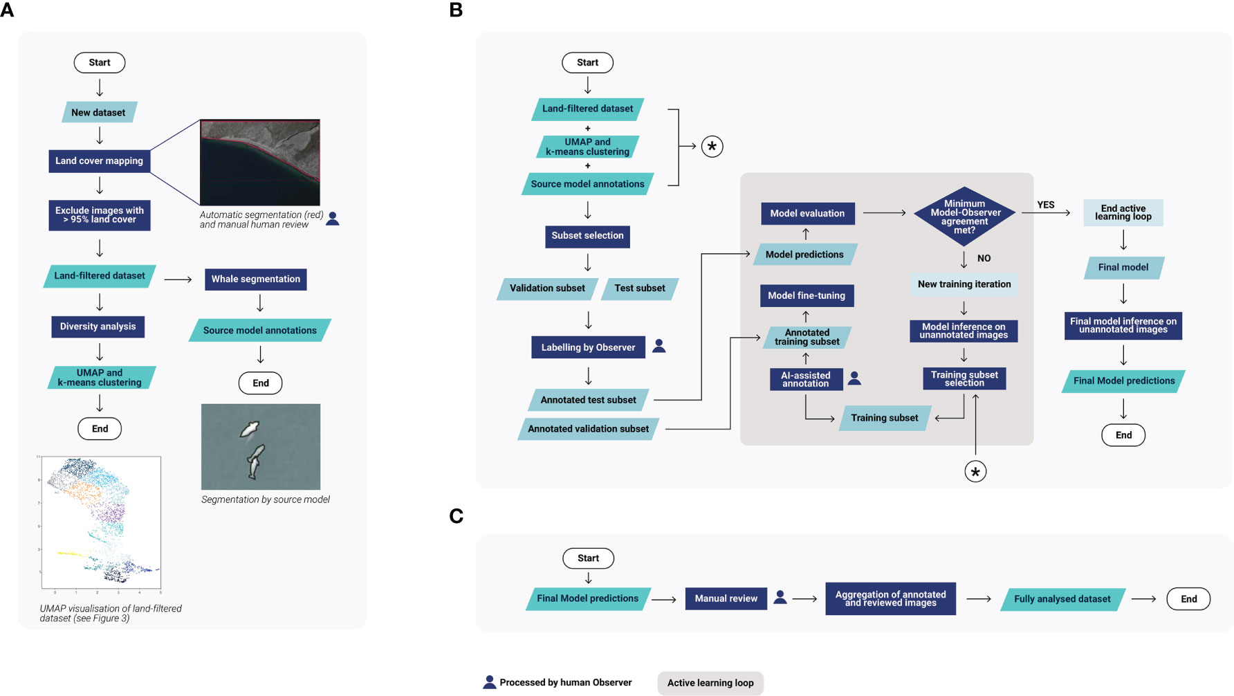
Figure 2 Overview of the human-in-the-loop pipeline. The pipeline is divided into three main stages: (A) The preliminary analysis, (B) The active learning loop, (C) The human review of the predictions.

In the entirety of this pipeline, the human annotator is involved in four tasks: (1) validating the segmentation of the land areas, (2) annotating validation and test images used to monitor the deep learning model, (3) annotating training images selected by active learning techniques, and (4) reviewing all predictions after the model’s final analysis.

2.2 Data specification

2.2.1 Study area

The aerial survey was designed to detect and monitor beluga whales of the Cumberland Sound population in Clearwater Fjord, Canada. This population is composed of roughly 1,400 individuals (Watt et al., 2021) who are believed to reside year-round in Cumberland Sound, an Arctic waterway, based on information derived from telemetry data of 14 individuals (Richard and Stewart, 2008). During the open-water season in summer a large portion of this population congregates in Clearwater Fjord, located at the northern end of the sound (66°34’ N, 67°26’ W).

2.2.2 Data collection

In 2017, DFO conducted a photographic survey of the Cumberland Sound beluga population from 29 July to 12 August. Surveys were performed using a twin-engine Havilland Twin Otter 300 plane, flying at 100-110 knots at a goal altitude of 610m. Photographic surveys were performed over Clearwater Fjord following 26 pre-determined parallel transect lines 700m apart oriented east-west. To collect photographs a Nikon D810 camera, with 25mm lens, was mounted and positioned straight down at the rear of the aircraft to capture photographs. The camera was linked to a GPS receiver and was set to capture one photograph every seven to eight seconds. Each photograph covered an area of about 875m x 585m, with a 20% overlap on consecutive and adjacent photographs along transects. The photographs were acquired over four days flying over the same area.

2.2.3 Manual data analysis

The 5334 photographs of the area of interest were first examined to detect belugas by a photo-analyst from DFO, called Observer 3 in this paper. The analyst examined the georeferenced photographs using ArcMap 10.1 software by Esri. Each image was scanned and upon detection of a beluga whale a point annotation was added to the target in the image. Observer 3 detected 4572 beluga occurrences within the dataset. All detections noted in our study are whale targets in the images we processed; we did not remove duplicate targets detected in the overlap portions of images or interpret any abundance of these whale populations. Those annotations were only used for comparison with the results of our human-in-the-loop pipeline, not for training the pipeline.

Since this fully manual analysis was not conducted within this study, the time spent analyzing the dataset has not been recorded. However, it can be estimated that between 1328 hours (8 months working at 8 hours a day) and 2016 hours (12 months at 8 hours a day) were needed to perform this task without AI-assistance.

2.3 Detailed pipeline for experiments

2.3.1 Preliminary analysis

2.3.1.1 Land cover mapping

To automatically exclude images containing only land from our analysis, and automatically dismiss any predictions falling on land, we performed AI-assisted annotation to get a binary land segmentation mask for each image of the dataset. The land segmentation model used had a UNet50-ResNeXt architecture, and was trained on a dataset of 11,702 images from similar, but non-overlapping, Arctic surveys. This dataset was split into training, validation, and test subsets with ratios of 70%, 15%, and 15% respectively. The model was trained for 11 epochs, with a learning rate of 2e-4. Loss was computed using the Log-Cosh Dice coefficient. Since this model was not fine-tuned on the new dataset, it made errors, especially in areas of shallow and muddy water, so we then manually vetted the predicted annotations, modifying any predictions that did not accurately reflect the observed coastlines.

2.3.1.2 Source whale model

A semantic segmentation model trained on another dataset, i.e., the source model, was used to find cetaceans in the first iteration. The source and new datasets differ in flight altitude, geographic area covered, and predominant species found. The source dataset was acquired by DFO in 2013, over the Canadian Arctic Archipelago, with a target flight altitude of about 305m. In 1562 images, 10,253 cetaceans were annotated. They consisted mostly of narwhals (about 80%), but also belugas (about 20%) and bowhead whales (less than 1%).

To train the source whale model, images from the source dataset were split into training, validation, and test subsets with ratios of 70%, 15%, and 15% respectively. This split was done randomly, but with the constraint that two images with a geospatial overlap could not be in different subsets, so as to prevent cross-contamination. A supervised training was carried out, using a U-Net architecture (Ronneberger et al., 2015), and with EfficientNet-b3 (Tan and Le, 2019) as an encoder. It was trained for 50 epochs with an initial learning rate of 2e-4. The optimizer used was AdamW and the loss was computed with the Dice coefficient. Of the 1658 whales in the 234 test images, 1568 were segmented by the model, giving a recall of 94.6% at 95.66% of precision. For more details on the metrics used, refer to the section 2.3.4 Metrics.

2.3.1.3 Diversity analysis

In order to minimize redundancy in the images sent for manual annotation, and hence the number of iterations to reach the stopping criterion, the automatic selection of the images to annotate was done in such a way that represented the diversity of oceanic environments seen across all images.

To do this, we first ran all the images in the dataset through an off-the-shelf pre-trained convolutional neural network (ResNet-50 (He et al., 2016) from TorchVision), and extracted the final activation layer after a forward pass through the network. The activation layer for each image was then fed into a nonlinear dimensionality reduction tool, UMAP (McInnes et al., 2018), which is designed to reduce the dimensionality of high-dimensional data, while retaining some of the meaningful characteristics of the data, such as similar elements clustering together across space. We chose to reduce the representation of each image to two dimensions, to enable human-readable visualizations (Figure 3). The two-dimensional representations did indeed cluster similar environmental conditions together in space, so that images dominated by land cover, shallow water, white caps, or muddy water, for instance, clustered in contiguous regions of the 2D space.

FIGURE 3

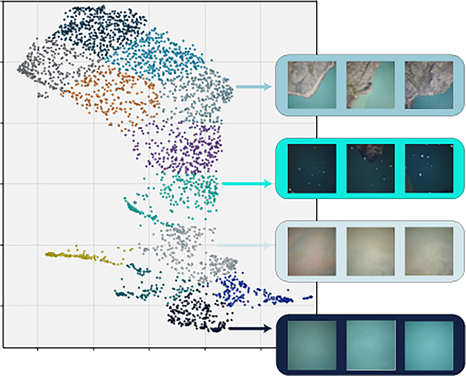
Figure 3 Clustered UMAP visualization of the new dataset. Each point represents an image and is color-coded by cluster. To illustrate the similarity of images within clusters, rectangles on the right show examples of three random images from four different clusters.

To use this information for image sampling and based on a visual assessment of the UMAP representation, we binned the images into 12 discrete clusters using the k-means clustering algorithm, assigning each image in the dataset an arbitrary number according to which environmental cluster it fell into. Using this representation, images were picked successively and randomly from the different clusters to obtain a representative selection of the environmental diversity.

2.3.2 Active learning pipeline

2.3.2.1 Subsets selection and annotation

2.3.2.1.1 Validation and test subsets

Creating validation and test subsets including whales was challenging, since no a priori knowledge on the dataset was used. Random sampling would have likely yielded subsets without any whales, and that did not represent the dataset’s true range of environmental diversity. For this reason, we relied on the preliminary analysis results. For each of the test and valid subsets, 50 images were selected successively and randomly, alternating between the different UMAP clusters to provide representative sampling of environmental diversity. The selection algorithm also ensured that two images with space-time overlap were not in different subsets. For 20 images of each subset, another selection rule was imposed using the predictions made by the source whale model: these images had to contain at least two predictions of whales scoring above 60% confidence to be selected. Although there is some bias in this approach since the source model’s predictions were used to select images for its own evaluation, it was the best way to ensure we included cetaceans in validation and testing, without having to manually evaluate the dataset. Since belugas live in groups, selecting an image with at least two predicted whales generally gave access to a larger group, including whales not detected by the model. Moreover, as the source model was not yet adapted to the target domain, the selections also included false positives. Using a selection of images that included not only true positives, but also false predictions enabled us to automatically create validation and test subsets capable of tracking the evolution of the model’s fine-tuning. Following the selection of images for the validation and test subsets, we proceeded to annotate them. One of the challenges of AI for wildlife monitoring is that the ground truth is based on human annotations, and therefore contains some degree of difference, owing to inter- and intra-observer variability. To calculate the variability of annotation between different expert marine mammal biologists, the test subset was analyzed independently by three observers (Table 1) (see section 2.3.4.2 Measuring agreement for further details). Only the test subset was analyzed by multiple observers as it contained a representative sample of environmental diversity of the full dataset and to limit the annotation workload. Observer 1, a Whale Seeker biologist, was the primary annotator, since in addition to the test subset, they also annotated the validation and train subsets, as well as doing the final prediction reviews. Observer 2 was also a Whale Seeker biologist. They both used the annotation software DIVE to draw individual polygons around each whale. Observer 3 was a DFO biologist who had previously annotated the entire dataset (see section 2.2.3 Manual analysis). Since the annotations from Observers 1 and 2 were individualized polygons while those from Observer 3 were points centered on the whales, we transformed these points into a 2*2 pixels square to allow comparison. Hence, a polygon intersecting a square is considered as a common annotation between observers.

TABLE 1

Table 1 Summary of annotations for the validation and test subsets according to the three observers.

Using the test-set annotations of the three observers, we calculated their inter-observer agreement, a key metric in a context where there is no real ground truth. This metric was used as the stopping criterion of the active learning loop: the loop would be ended once the agreement between the model predictions and the human annotations equaled or exceeded this value.

2.3.2.1.2 Training subsets

At each iteration, 50 images were selected to be annotated for fine-tuning. To sample images with the most uncertain targets, we used the least confidence criterion (Monarch et al., 2021) to select 20 images based on the confidence score of the predicted targets. An additional 25 images were selected using a most confidence criterion. This criterion is based on the number of targets in an image with a confidence above a specified threshold value, in this case 90%. This criterion had the advantage of generating true whale predictions that can be easily transformed into annotations when the segmentation has a high enough quality. It also allowed us to catch false positives with a high level of confidence, a frequent occurrence when analyzing new environments. Since we were selecting entire images and not just targets, this criterion provided access to a large number of beluga whales, and thereby potentially to false negatives. Finally, five images were also randomly selected for annotation. To avoid redundancy of information, we used the UMAP representation to select the images.

The annotation was performed by Observer 1 with the model’s assistance, i.e., the observer had access to the predictions of the model to speed up analysis. To enrich the pool of negative examples sent to the model during training, we followed a hard negative mining approach, which means we transformed the false positives from selected images into negative examples for the next training iteration. Since the dataset images measured 7360 per 4912 pixels — too large to be fed directly into machine learning algorithms — tiles of 256 per 256 pixels were extracted around each whale and hard negative example. To complete the dataset, negative tiles were also extracted randomly. To avoid an unbalanced dataset, the same number of positive and negative tiles were fed to the model. Because positive examples are typically scarce in cetacean surveys, 750 positive examples from the source dataset were also selected randomly to supplement those from the new dataset. A summary of the data used in each iteration can be found in Table 2.

TABLE 2

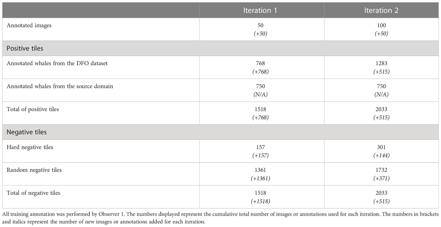
Table 2 Summary of the data used in each training iteration.

2.3.2.2 Model fine-tuning

A complete fine-tuning of the previously trained model was performed on each iteration. For the first iteration, the starting point was the source model. We used a U-Net architecture with an EfficientNet-B3 encoder. During each training phase, several runs were performed with different random seed states. Since the human annotator only verifies images that contain at least one whale prediction, we needed a fairly sensitive model. For each iteration, between all the models from the different runs, we chose the model with the best recall for an accuracy over 85%. More details about the hyperparameter values used can be found in Table 3.

TABLE 3

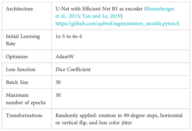
Table 3 Hyperparameters used to fine-tune the model.

2.3.3 Human review of predictions

Once the stopping criterion was reached, the final iteration of the model was used for inference on all remaining unannotated images. The list of images with at least one whale detected was then sent to Observer 1 for manual revision. During this process, the observer could approve, remove, or correct the predictions. They could also add targets not predicted by the model, and separated groups of whales that were segmented as one by the model, to facilitate an individual count of the number of cetaceans.

2.3.4 Metrics

2.3.4.1 Computer vision metrics

To evaluate the performance of the models, precision (Eq. 1), recall (Eq. 2), and F1-score (Eq. 3) were calculated. For our application, since it was not the quality of the segmentations that was important but rather binary detection quality, these three metrics were computed not at the pixel but at the target level. Each group of contiguous positive pixels was considered a target. Each whale prediction that intersected a human annotation was counted as a true positive. Recall is the most critical metric for this application since we focus on missing as few individuals as possible. High precision is nonetheless important so that the observer does not spend too much time checking for false positives.

$\begin{array}{ll}Precision= \frac{True Positives}{True Positives + False Positives} & (1)\end{array}$

$\begin{array}{ll}Recall= \frac{True Positives}{True Positives + False Negatives}& (2)\end{array}$

$\begin{array}{ll}F1-Score= \frac{2 \times Precision \times Recall}{Precision + Recall}& (3)\end{array}$

2.3.4.2 Measuring agreement

One challenge of quantifying automated approach success using remote detection is the inherent variability in ground-truth data, both between expert human observers and within the same observer. Numerous studies across various taxa have measured inter-observer variability in overall animal counts given the same remote sensing imagery (Linchant et al., 2015; Wanless et al., 2015; Schlossberg et al., 2016; Fossette et al., 2021). These studies report count discrepancies in the range of 5 - 15%. Disagreement across matched detections (rather than the overall count) is less well documented but is likely significantly higher.

This range of inter-observer variability, even among experts, makes 100% recall and precision a moving target, and not a realistic or desirable goal for automated or manual approaches. Instead, an automated solution’s recall and precision can instead be interpreted as the algorithm’s “agreement” with the observer who created the ground-truth annotations, and can be expected, at best, to approach the agreement values human experts have with respect to one another. Specifically, we defined agreement between two observers (human or computer) as the intersection over union (IOU) between them, which is the number of shared detections divided by the size of the union of the two observer’s detections (Eq. 4).

$\begin{array}{ll}Inter - observer agreement=\frac{ Detection{s}_{ObsA, ObsB} }{ Detection{s}_{ObsA, ObsB} + Detection{s}_{ObsA} + Detection{s}_{ObsB}}& (4)\end{array}$

Where Detections_{ObsA, ObsB} represents the number of whales detected by both observers, while Detections_ObsA represents the number of detections made only by Observer A, and Detections_ObsB represents the number of detections made only by Observer B.

We chose this metric since, unlike concepts such as recall and precision, it is symmetric between the two observers, rather than assuming one to be ground truth.

3 Results

3.1 Land cover exclusion

Using the land use mapping done in the preliminary analysis, 1977 images (37% of the total) were excluded from further analysis because they were covered by more than 95% land, leaving 3357 images to be analyzed for whales.

3.2 Evaluation on the test subset

3.2.1 Inter-observer agreement

The number of whales found in the 50 test images varied between observers. Observer 1 was the most conservative annotator, disregarding targets that were deep in the water column, whereas Observer 3 was less conservative and included deep-water targets. Therefore, the number of whales detected in the 50 images ranged between 239 to 315. The percentage of agreement between pairs of observers ranged from 88.5% to 92.88% (Table 4).

TABLE 4

Table 4 Annotation agreement on the test subset between the three observers.

Most of the disagreements between observers concerned targets that might be whales swimming deep in the water column (Figures 4A, B). Some discrepancies were due to targets resembling waves (Figure 4C) or birds (Figure 4D).

FIGURE 4

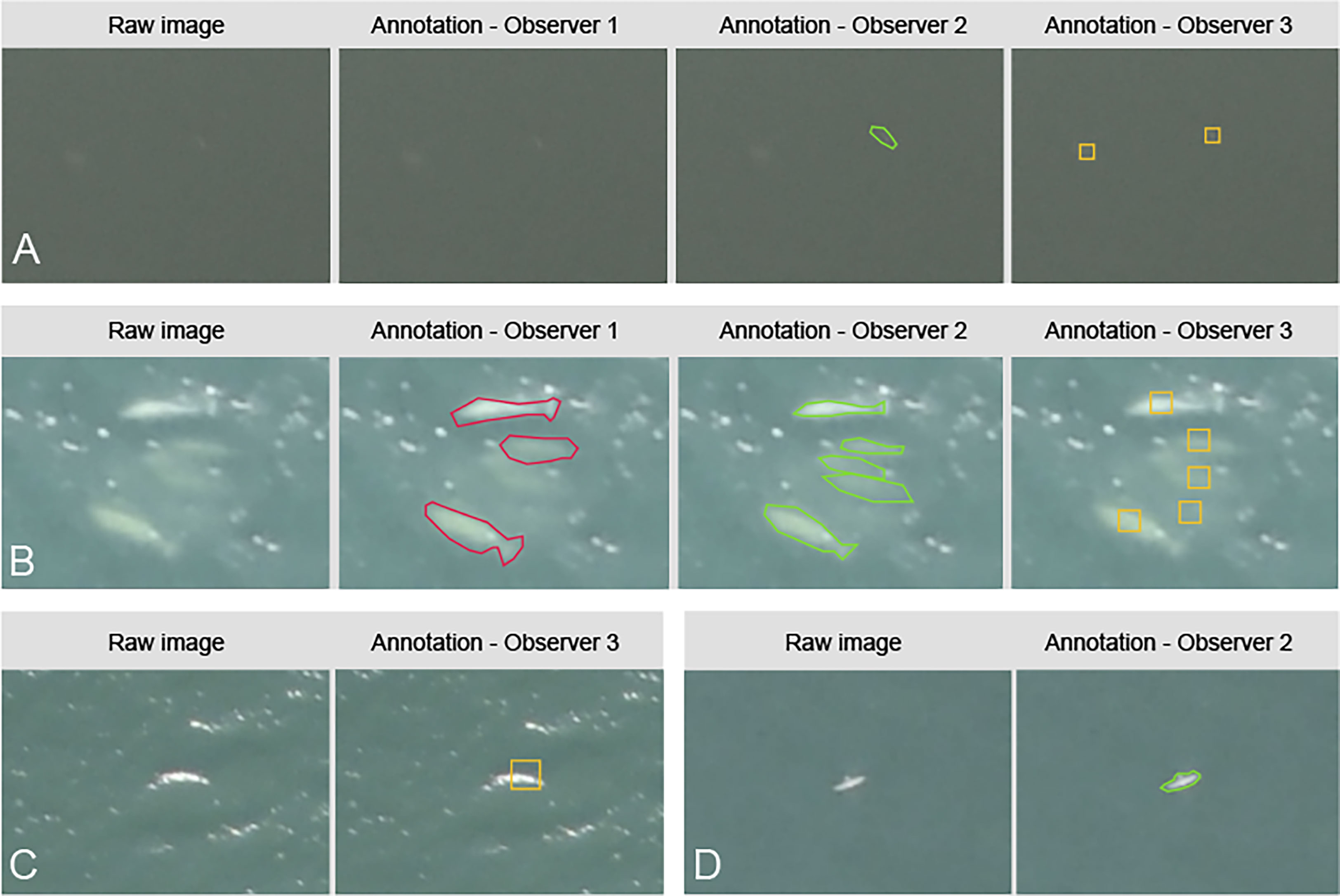
Figure 4 Examples of annotation disagreement in the test subset. (A, B) Targets annotated differently by each observer with red outlines for Observer 1, green outlines for Observer 2, and yellow boxes for Observer 3. (C) Target annotated only by Observer 3. (D) Target annotated only by Observer 2.

3.2.2 Active learning loop performance

Two iterations, totaling 100 annotated images (~2% of the complete dataset), enabled the model to exceed the minimum inter-observer agreement value on the test subset, with model–observer agreement percentages ranging from 90.03% to 91.37% (Table 5; Figure 5).

TABLE 5

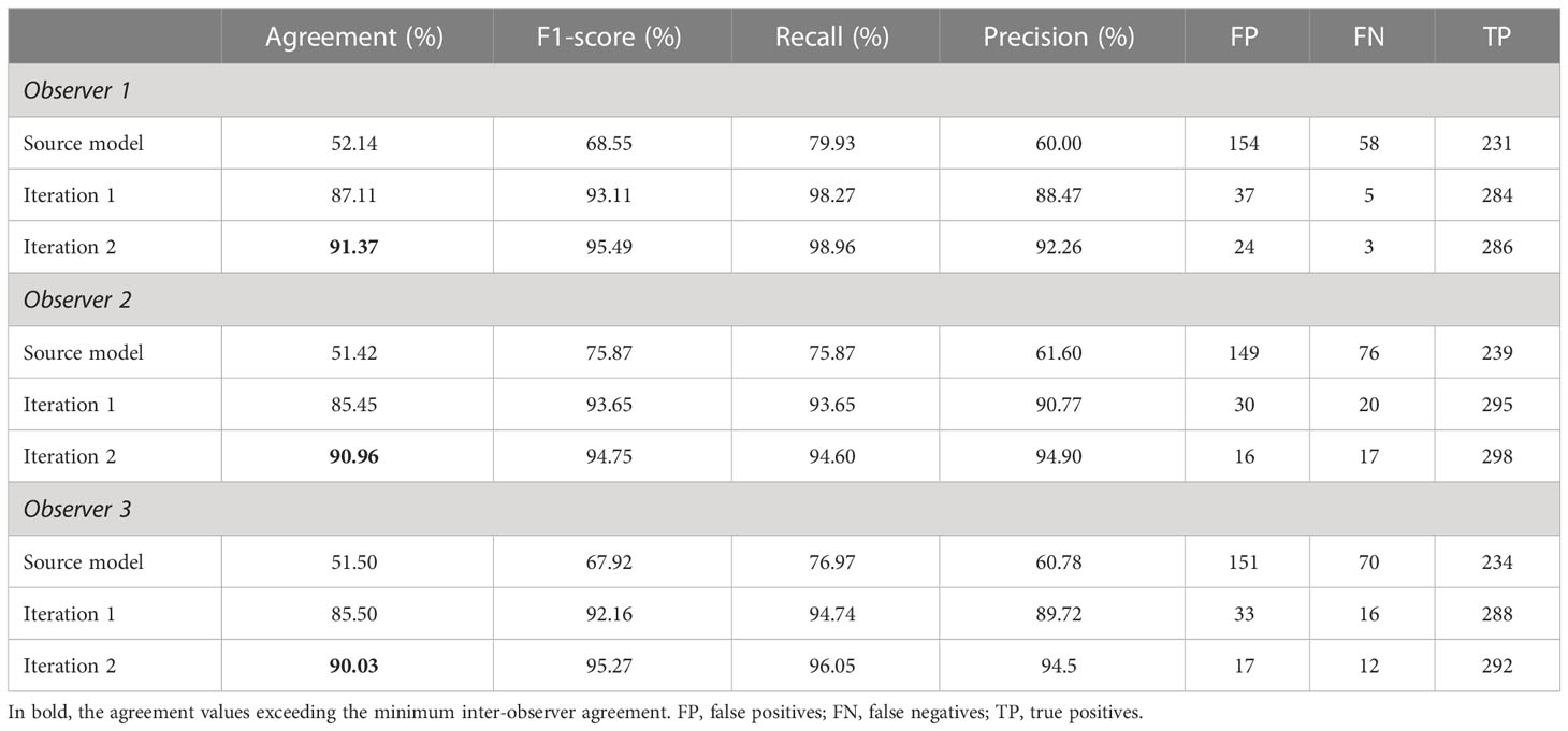
Table 5 Summary of the results between the model and the three observers on the test subset.

FIGURE 5

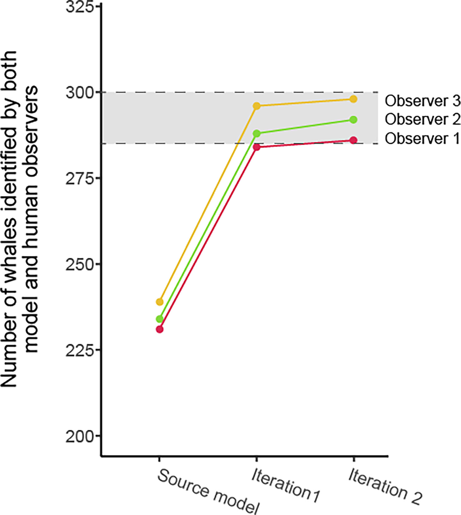
Figure 5 Evolution of the observer–model whale detection agreement on the test subset through the model training iterations. The shaded area between hash lines indicates the inter-observer minimum and maximum whale detection agreement.

Despite differences between the source and new datasets, the source model provided an initial recall on the test subset ranging from 75.87% to 79.93% depending on the observer. The incorporation of target domain annotations greatly improved the detection capabilities: the number of false negatives shrank more than sixfold between the source model and the iteration 1 model. After iteration 2, the recall ranged from 94.75% to 98.96%. Interestingly, across all the false negatives, none had consensus by all three observers, highlighting the alignment between inter-observer discrepancies and model-observer discrepancies. Precision increased by an average of 28.8 percentage points after 50 annotated images were added. This upward trend continued less steeply between iteration 1 and 2, with an average gain of 4.23 percentage points. After iteration 1, some of the false positives were recognizable objects like rocks, glare effects and waves, but after iteration 2, the false positives related to objects that we couldn’t identify. All three observers agreed on only 7 of the false positives, and some of them could indeed be belugas that were missed by all three (Figure 6).

FIGURE 6

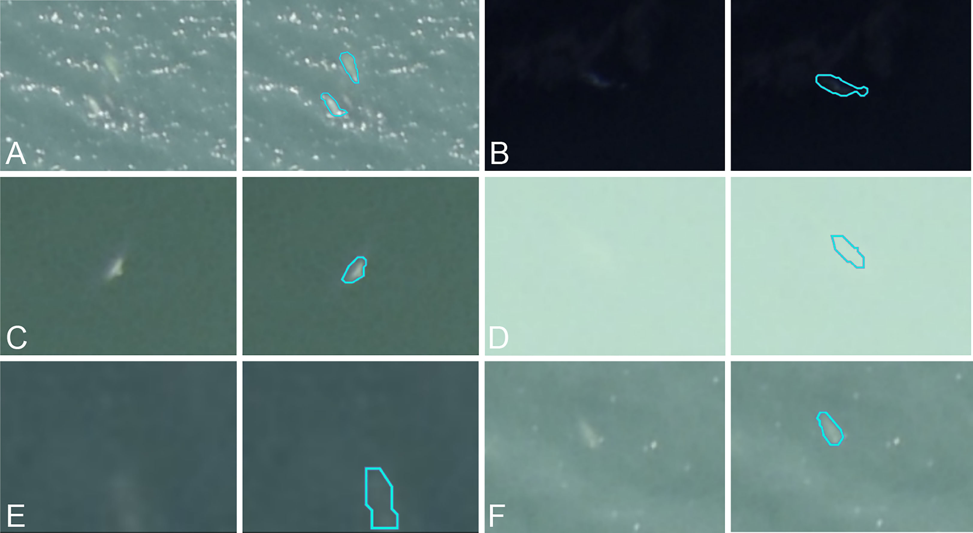
Figure 6 (A–F) Examples of predictions (original image on left, turquoise outline prediction on right) from iteration 2 identified as false positives for all three observers.

3.3 Evaluation on the whole dataset

Once the active learning loop was complete, Observer 1 proceeded to the final step of the pipeline: reviewing the predictions on the remaining 3157 images that had not been manually annotated. In this review, 572 predictions were removed, and 58 detections were added.

The annotations from the human-in-the-loop pipeline were then compared with those made without AI assistance by Observer 3. In total, 4298 belugas were detected by the pipeline, while the Observer 3 detected 4572 belugas, a difference of 274 individuals. The level of mutual agreement reached 84%, representing 4051 mutual detections. Observer 1 detected 247 belugas that were not detected by Observer 3, and Observer 3 detected 521 belugas that were not detected by Observer 1.

As no third-party biologist reviewed the disagreements, we were not able to arbitrate on the presence or absence of belugas. Nevertheless, to better understand the disagreements between the human-in-the-loop pipeline and Obsrver 3 detections, Observer 1 manually inspected the discrepancies.

Out of the 768 targets in disagreement, he assessed that 60% of them could not be annotated with certainty, due to a lack of visibility, related to the turbidity of the water, the conditions at sea, and especially, to the depth of the detected target (Figure 7). While image annotation protocols generally specify a maximum depth for a target to be counted as a whale, in practice it is difficult to follow these guidelines, which leaves room for some interpretation. When analyzing groups of whales, we noticed that observers were inclined to annotate targets at great depths as belugas, while similar targets outside whale groups were not annotated as such. About 35% of the uncertain targets were found in beluga whale groups. The proximity of the belugas and the turbulence they create rendered individualization difficult (Figure 7).

FIGURE 7

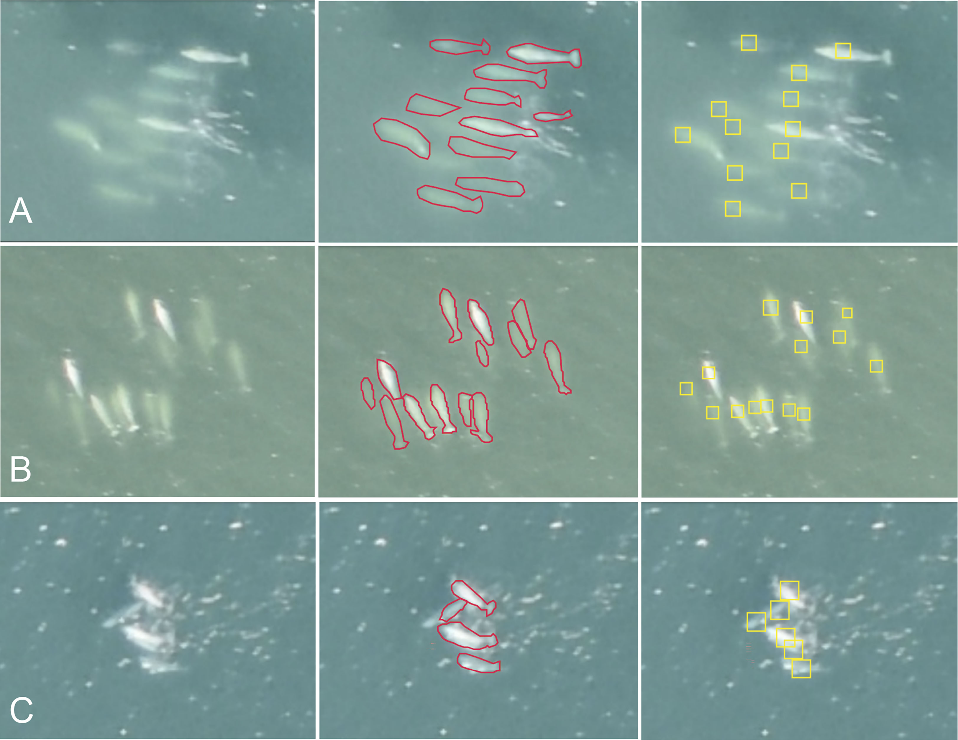
Figure 7 Examples of annotation disagreements between Observer 1 (middle, in red) and Observer 3 (right, in yellow). Original unannotated image on left. Total count of belugas in (A) Observer 1: 11, Observer 3: 12; (B) Observer 1: 13, Observer 3: 14; (C) Observer 1: 4, Observer 3: 6.

3.4 Time-tracking

We tracked the time spent by Observer 1 annotating images and reviewing predictions to estimate the time needed for an observer to analyze a dataset while being assisted by the human-in-the-loop pipeline (Figure 8). In total, 53 hours were spent for the complete analysis of this dataset of 5534 images. The AI-assisted annotation of the land took approximately 23 hours, given that about 80% of the images included land. Whale detection required approximately 31 hours of manual work to analyze the eligible 3357 images (i.e., with a land cover under 95%). Given that a fully manual analysis took an estimated 1328 to 2016 hours, the time savings for the observer using our AI-assisted approach are in the range of 96-97%.

FIGURE 8

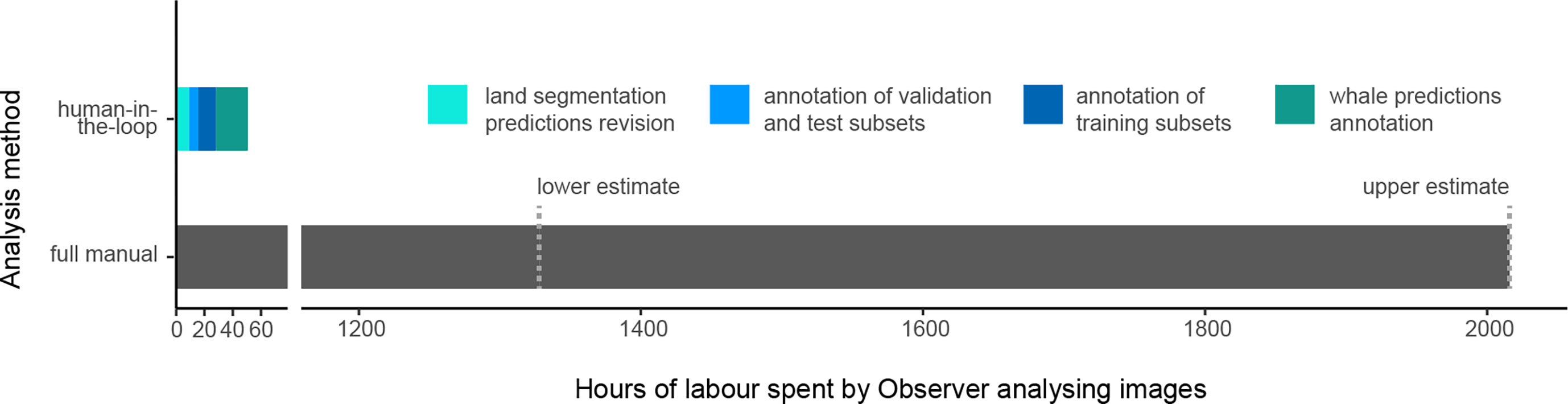
Figure 8 Comparison of the time spent by Observer 1 to analyze the dataset with the AI-assisted approach versus the time spent by Observer 3 to analyze the dataset fully by hand. The exact time spent for the full manual analysis was not recorded, hence the lower and upper estimates of the time needed to analyze a dataset of 5334 images.

4 Discussion

4.1 Scaling the adoption of AI for aerial whale monitoring

Our study presents an original deep learning-based solution using a human-in-the-loop framework to detect whales from aerial imagery. AI-assisted detection can process imagery significantly faster than manual detection, thereby providing more time for interpretation and development of mitigation strategies. Manual analysis of a survey can take months or years, delaying evaluation of mitigation plans, which can be detrimental to the species of interest.

Although there has been previous work using deep learning to analyze imagery of marine mammals, they have not yet gained traction with the global community of wildlife managers and other ocean stakeholders. While data democratization is often put forward as a roadblock to implement AI solutions in ecology (Ditria et al., 2022), another major challenge is the lack of knowledge sharing and understanding between AI experts and wildlife managers. Creating a widespread usable framework not only requires deep expertise and communication from multiple disciplines such as computer science and ecology, but also the involvement of all marine stakeholders.

Full photographic surveys are desirable in the field because they are cost-effective, requiring fewer personnel, which also means less human risk; however, processing vast amounts of imagery that are acquired is a major bottleneck. Our methodology, including the use of UMAP to select the most impactful data for re-training, helps to make full photographic surveys a viable monitoring solution, by cutting down the number of manual annotations needed for re-training.

Since each dataset is different, it is expected that the time an expert spends on each AI-assisted analysis will vary. The greatest time savings will likely be for repeated surveys from one year to the next, or for analyzing historical datasets, where the target species and geographic area are constant.

4.2 The need of standardization and transparency

By analyzing a dataset with a single model, AI improves standardization: each image is processed identically, without the biases and variability that can occur during manual annotation. However, this approach does not mean we can do without observers’ intervention: their expertise is required for fine-tuning data as well as prediction verification. Therefore, the consistency of an AI solution is limited by the consistency of manual interventions and establishing a robust manual annotation protocol from the outset is essential, especially regarding common conditions for inter-observer discrepancy such as deep targets and murky water. Standardization of protocols for assessing difficult cases would ensure temporally spaced surveys are consistent, even if they cannot be ground-truthed. As the AI-assisted annotation process greatly reduces the time taken by observers to analyze the images, multiple observers could be asked to review the annotations and arbitrate the difficult cases. Because marine mammal management often has large environmental, monetary, and cultural implications, a standardized approach offers transparency for stakeholders and can go a long way to developing trust in the scientific process.

4.3 AI perspectives

Improvements can be made to the pipeline presented here. Going from semantic segmentation to an approach that isolates individuals could speed up the manual revision process. However, this approach needs to be robust to the proximity, and even overlap, of individuals. Developing a source model with a higher generalization capacity would also be an improvement since better pre-analysis requires fewer active learning iterations. Improving generalization remains an area of ongoing research (Wang et al., 2021). Developing specialized source models for given species and geographic areas could also improve the pre-analysis results. Finally, extending the model’s scope from whale detection to species identification would allow for better monitoring of multiple species within the same geographical area.

5 Conclusion

In this study, we proposed and applied a human-in-the-loop approach to address the challenge of a real-world cetacean monitoring application case: analyzing a novel dataset of aerial images for beluga whale monitoring. Through this approach and the close collaboration between AI and the observer, expert-quality analysis was quickly provided for the 5334 images in the dataset, with only 100 annotated images for training. Generalization of this approach to aerial image analysis could significantly improve cetacean monitoring in quantity and quality. Keeping the expert in the loop ensures human-level quality results and better adaptation to new environmental and biological conditions in the imagery. Using computing power instead of total human analysis also allows more data to be analyzed in a dramatically shorter time period, allowing more meaningful time sensitive decisions. Improvements can still be made to the proposed method, both for AI (better generalization of source models, multi-species identification) and for cetacean monitoring methodology (standardized taxonomy and image annotation protocol), and yet the human-in-the-loop approach proposed here constitutes a first innovative and practical solution for automating imagery analysis for cetacean monitoring.

Data availability statement

The data analyzed in this study is subject to the following licenses/restrictions: Crown Copyright. Requests to access these datasets should be directed to CW, cortney.watt@dfo-mpo.gc.ca.

Author contributions

JB, MK, ET and AG-T conceived the ideas. JB, MK, and AG-T designed the methodology. MM and CW collected the data. BC and RF annotated manually the data. JB, MK and AG-T implemented the designed methodology and proceeded to the automatic analysis of the dataset. JB, BC, ET and MK led the writing of the manuscript. All authors contributed to the article and approved the submitted version.

Funding

The Polar Continental Shelf Program, Fisheries and Oceans Canada, Species at Risk and the Nunavut Wildlife Management Board financially supported imagery acquisition. Whale Seeker financially supported the data analyses.

Acknowledgments

Thanks to L. Montsion for manual image annotation. Thanks to the community of Pangnirtung, the Pangnirtung Hunters and Trappers Association, C. Matthews, B. Dunn, M. Ghazal, and C. Hornby for photographic acquisition.

Conflict of interest

Authors JB, MK, and RF are employed by Whale Seeker, a B-corp company specialized in marine mammal detection that was founded by authors BC, AG-T and ET. Whale Seeker sells an image analysis service for the detection of marine mammals whose artificial intelligence-assisted annotation tool, Mobius, is associated with this research.

The remaining authors declare that the research was conducted in the absence of any commercial or financial relationships that could be construed as a potential conflict of interest.

The reviewer AB declared a past collaboration with the author ET to the handling editor.

Publisher’s note

All claims expressed in this article are solely those of the authors and do not necessarily represent those of their affiliated organizations, or those of the publisher, the editors and the reviewers. Any product that may be evaluated in this article, or claim that may be made by its manufacturer, is not guaranteed or endorsed by the publisher.

References

Berg P., Santana Maia D., Pham M.-T., Lefèvre S. (2022). Weakly supervised detection of marine animals in high resolution aerial images. Remote Sens. 14, 339. doi: 10.3390/rs14020339

CrossRef Full Text | Google Scholar

Borowicz A., Le H., Humphries G., Nehls G., Höschle C., Kosarev V., et al. (2019). Aerial-trained deep learning networks for surveying cetaceans from satellite imagery. PloS One 14, e0212532. doi: 10.1371/journal.pone.0212532

PubMed Abstract | CrossRef Full Text | Google Scholar

Caughley G. (1974). Bias in aerial survey. J. Wildlife Manage. 38, 921–933. doi: 10.2307/3800067

CrossRef Full Text | Google Scholar

Charry B., Marcoux M., Cardille J. A., Giroux-Bougard X., Humphries M. M. (2020). Hierarchical classification of narwhal subpopulations using social distance. J. Wildlife Manage. 84, 311–319. doi: 10.1002/jwmg.21799

CrossRef Full Text | Google Scholar

Charry B., Marcoux M., Humphries M. M. (2018). Aerial photographic identification of narwhal (Monodon monoceros) newborns and their spatial proximity to the nearest adult female. Arctic Sci. 4, 513–524. doi: 10.1139/as-2017-0051

CrossRef Full Text | Google Scholar

Charry B., Tissier E., Iacozza J., Marcoux M., Watt C. A. (2021). Mapping Arctic cetaceans from space: A case study for beluga and narwhal. PloS One 16, e0254380. doi: 10.1371/journal.pone.0254380

PubMed Abstract | CrossRef Full Text | Google Scholar

Cubaynes H. C., Fretwell P. T., Bamford C., Gerrish L., Jackson J. A. (2019). Whales from space: Four mysticete species described using new VHR satellite imagery. Mar. Mammal Sci. 35, 466–491. doi: 10.1111/mms.12544

CrossRef Full Text | Google Scholar

Ditria E. M., Buelow C. A., Gonzalez-Rivero M., Connolly R. M. (2022). Artificial intelligence and automated monitoring for assisting conservation of marine ecosystems: A perspective. Front. Mar. Sci. 9, 918104. doi: 10.3389/fmars.2022.918104

CrossRef Full Text | Google Scholar

Fossette S., Loewenthal G., Peel L. R., Vitenbergs A., Hamel M. A., Douglas C., et al. (2021). Using aerial photogrammetry to assess stock-wide marine turtle nesting distribution, abundance and cumulative exposure to industrial activity. Remote Sens. 13, 1116. doi: 10.3390/rs13061116

CrossRef Full Text | Google Scholar

Fretwell P. T., Staniland I. J., Forcada J. (2014). Whales from space: Counting southern right whales by satellite. PloS One 9, e88655. doi: 10.1371/journal.pone.0088655

PubMed Abstract | CrossRef Full Text | Google Scholar

Gheibi M. (2021). Helping biologists find whales: AI-in-the-Loop support for environmental dataset creation (Halifax, Canada: Dalhousie University). (Master thesis).

Google Scholar

Gray P. C., Bierlich K. C., Mantell S. A., Friedlaender A. S., Goldbogen J. A., Johnston D. W. (2019). Drones and convolutional neural networks facilitate automated and accurate cetacean species identification and photogrammetry. Methods Ecol. Evol. 10, 1490–1500. doi: 10.1111/2041-210X.13246

CrossRef Full Text | Google Scholar

Guirado E., Tabik S., Rivas M. L., Alcaraz-Segura D., Herrera F. (2019). Whale counting in satellite and aerial images with deep learning. Sci. Rep. 9, 14259. doi: 10.1038/s41598-019-50795-9

PubMed Abstract | CrossRef Full Text | Google Scholar

He K., Zhang X., Ren S., Sun J. (2016). “Deep residual learning for image recognition, in: 2016 IEEE conference on computer vision and pattern recognition (CVPR),” in Presented at the 2016 IEEE Conference on Computer Vision and Pattern Recognition (CVPR), IEEE, Las Vegas, NV, USA. 770–778. doi: 10.1109/CVPR.2016.90

CrossRef Full Text | Google Scholar

Heide-Jørgensen M. P. (2004). Aerial digital photographic surveys of narwhals, monodon monoceros, in northwest Greenland. Mar. Mammal Sci. 20, 246–261. doi: 10.1111/j.1748-7692.2004.tb01154.x

CrossRef Full Text | Google Scholar

Kellenberger B., Marcos D., Lobry S., Tuia D. (2019). Half a percent of labels is enough: Efficient animal detection in UAV imagery using deep CNNs and active learning. IEEE Trans. Geosci. Remote Sens. 57, 9524–9533. doi: 10.1109/TGRS.2019.2927393

CrossRef Full Text | Google Scholar

Lee P. Q., Radhakrishnan K., Clausi D. A., Scott K. A., Xu L., Marcoux M. (2021). Beluga whale detection in the Cumberland sound bay using convolutional neural networks. Can. J. Remote Sens. 47, 276–294. doi: 10.1080/07038992.2021.1901221

CrossRef Full Text | Google Scholar

Linchant J., Lhoest S., Quevauvillers S., Semeki J., Lejeune P., Vermeulen C. (2015). Wimuas: Developing a tool to review wildlife data from various uas flight plans. ISPRS - Int. Arch. Photogrammetry Remote Sens. Spatial Inf. Sci. XL3, 379–384. doi: 10.5194/isprsarchives-XL-3-W3-379-2015

CrossRef Full Text | Google Scholar

Mackenzie D. I., Nichols J., Sutton N., Kawanishi K., Bailey L. L. (2005). Improving inferences in population studies of rare species that are detected imperfectly. Ecology 86, 1101–1113. doi: 10.1890/04-1060

CrossRef Full Text | Google Scholar

McInnes L., Healy J., Saul N., Großberger L. (2018). UMAP: Uniform manifold approximation and projection. J. Open-Source Software 3, 861. doi: 10.21105/joss.00861

CrossRef Full Text | Google Scholar

Miao Z., Liu Z., Gaynor K. M., Palmer M. S., Yu S. X., Getz W. M. (2021). Iterative human and automated identification of wildlife images. Nat. Mach. Intell. 3, 885–895. doi: 10.1038/s42256-021-00393-0

CrossRef Full Text | Google Scholar

Monarch M., Munro R., Monarch R. (2021). Human-in-the-Loop machine learning: Active learning and annotation for human-centered AI. Simon Schuster.

Google Scholar

Pershing A. J., Christensen L. B., Record N. R., Sherwood G. D., Stetson P. B. (2010). The impact of whaling on the ocean carbon cycle: Why bigger was better. PloS One 5, e12444. doi: 10.1371/journal.pone.0012444

PubMed Abstract | CrossRef Full Text | Google Scholar

Pollock K. H., Kendall W. L. (1987). Visibility bias in aerial surveys: A review of estimation procedures. J. Wildlife Manage. 51, 502–510. doi: 10.2307/3801040

CrossRef Full Text | Google Scholar

Ren P., Xiao Y., Chang X., Huang P.-Y., Li Z., Gupta B. B., et al. (2021). A survey of deep active learning. ACM Comput. Surv. 54, 180:1–180:40. doi: 10.1145/3472291

CrossRef Full Text | Google Scholar

Richard P., Stewart D. B. (2008). Information relevant to the identification of critical habitat for Cumberland sound belugas (Delphinapterus leucas) (No. 2008/085) (Canadian Science Advisory Secretariat).

Google Scholar

Rodofili E. N., Lecours V., LaRue M. (2022). Remote sensing techniques for automated marine mammals detection: A review of methods and current challenges. PeerJ 10, e13540. doi: 10.7717/peerj.13540

PubMed Abstract | CrossRef Full Text | Google Scholar

Ronneberger O., Fischer P., Brox T. (2015). “U-Net: Convolutional networks for biomedical image segmentation,” in Medical image computing and computer-assisted intervention – MICCAI 2015, lecture notes in computer science. Eds. Navab N., Hornegger J., Wells W. M., Frangi A. F. (Cham: Springer International Publishing), 234–241. doi: 10.1007/978-3-319-24574-4_28

CrossRef Full Text | Google Scholar

Schlossberg S., Chase M. J., Griffin C. R. (2016). Testing the accuracy of aerial surveys for Large mammals: An experiment with African savanna elephants (Loxodonta africana). PloS One 11, e0164904. doi: 10.1371/journal.pone.0164904

PubMed Abstract | CrossRef Full Text | Google Scholar

Shah K., Ballard G., Schmidt A., Schwager M. (2020). Multidrone aerial surveys of penguin colonies in Antarctica. Sci. Robotics 5, eabc3000. doi: 10.1126/scirobotics.abc3000

CrossRef Full Text | Google Scholar

Tan M., Le Q. (2019). “EfficientNet: Rethinking model scaling for convolutional neural networks, in: Proceedings of the 36th international conference on machine learning,” in Presented at the International Conference on Machine Learning (Long Beach, CA, USA: PMLR). 6105–6114. doi: 10.48550/arXiv.1905.11946

CrossRef Full Text | Google Scholar

Tuia D., Kellenberger B., Beery S., Costelloe B. R., Zuffi S., Risse B., et al. (2022). Perspectives in machine learning for wildlife conservation. Nat. Commun. 13 (1), 792. doi: 10.1038/s41467-022-27980-y

PubMed Abstract | CrossRef Full Text | Google Scholar

Wang J., Lan C., Liu C., Ouyang Y., Qin T. (2021). “Generalizing to unseen domains: A survey on domain generalization,” in Presented at the Thirtieth International Joint Conference on Artificial Intelligence, Montreal, Canada. 4627–4635. doi: 10.24963/ijcai.2021/628

CrossRef Full Text | Google Scholar

Wanless S., Murray S., Harris M. P. (2015). Aerial survey of northern gannet (Morus bassanus) colonies off NW Scotland 2013 - NERC open research archive (No. 696). Scottish Natural Heritage.

Google Scholar

Watt C. A., Marcoux M., Hammill M., Montsion L., Hornby C., Charry B., et al. (2021). Abundance and total allowable landed catch estimates from the 2017 aerial survey of the Cumberland sound beluga (Delphinapterus leucas) population (No. 2021/50) (Canadian Science Advisory Secretariat (CSAS).

Google Scholar

Weinstein B. G. (2018). A computer vision for animal ecology. J. Anim. Ecol. 87, 533– 545. doi: 10.1111/1365-2656.12780

PubMed Abstract | CrossRef Full Text | Google Scholar

Wilkinson T., Agardy T., Perry S., Rojas L., Hyrenbach D., Morgan K., et al. (2003). “Marine species of common conservation concern. protecting species at risk across international boundaries,” in Presented at the Fifth International SAMPAA (Science and Management of Protected Areas), University of Victoria, Victoria, B.C., Canada.

Google Scholar

Yoccoz N. G., Nichols J. D., Boulinier T. (2001). Monitoring of biological diversity in space and time. Trends Ecol. Evol. 16, 446–453. doi: 10.1016/S0169-5347(01)02205-4

CrossRef Full Text | Google Scholar