Evaluation of the sensitivity on mesoscale eddy associated with the sea surface height anomaly forecasting in the Kuroshio Extension

The sensitivity of the sea surface height anomaly (SSHA) forecasting on the accuracy of mesoscale eddies over the Kuroshio Extension region, which was determined by the conditional non-linear optimal perturbation (CNOP) method using a two-layer quasigeostrophic model, is evaluated by adopting multiply realistic marine datasets through an advanced particle filter assimilation method. It is shown that, if additional observations are preferentially assimilated to the sensitive area of mesoscale eddies identified by the CNOP, where the eddies present a clear high- to low-velocity gradient along the eddy rotation, the forecasting skill of the SSHA can be more significantly improved. It is also demonstrated that the forecasts of the SSHA in the region where the large-scale mean flow possesses much stronger barotropic and/or baroclinic instability tend to exhibit stronger sensitivity to the accuracy of the initial field in the sensitive area of mesoscale eddies. Therefore, more attention should be preferentially paid to the assimilation of the additional observations of the mesoscale eddies for the SSHA forecast in the region with a strong velocity shear of ocean circulation. The present study verifies the sensitivity on mesoscale eddies of SSHA forecasts derived by the two-layer quasigeostrophic model using multiply sets of realistic oceanic data, especially including observation and reanalysis data, which further additionally demonstrates the importance of targeted observations of mesoscale eddies to the SSHA forecast in the regions of strong velocity shear of ocean circulation and provides a more credible scientific basis for the field campaign of the targeted observations for mesoscale eddies associated with the SSHA forecasting.

1 Introduction

Sea surface height anomaly (SSHA) is considered one of the features for the surface and subsurface dynamics of the ocean and directly or indirectly reflects information on the main dynamic processes, including mesoscale eddies, waves, currents, and tides (Tanajura et al., 2016; Song et al., 2021). The SSHA has provided a wealth of information about ocean circulation and atmosphere–ocean interactions (Tandeo et al., 2014). The forecasting of SSHA is crucial for predicting future extreme or very hazardous phenomena such as extremely high waves, hurricanes, and other phenomena (Tanajura et al., 2015). Highly accurate SSHA forecasts will also be allowed to provide a sufficient basis for ship navigation, marine engineering, and industrial development, as well as fishery resources forecast (Solanki et al., 2015; Lumban-Gaol et al., 2017). Currently, the study on the SSHA assimilation and, thus, highly accurate SSHA prediction has been a hot topic in physical oceanography and meteorological sciences (Tanajura et al., 2015; Yavuzdoğan and Tanır Kayıkçı, 2020).

The prediction of SSHA has Is been a challenge (Song et al., 2021). For decades, numerical models based on dynamical/physical equations have played a dominant role in ocean predictions and are also often used to predict SSHA. The data assimilation method can provide more accurate initial conditions for numerical models by combining limited observations and model output, thus increasing the medium- and short-term prediction skills of the model. Many studies have been devoted to the studies on the assimilation of SSHA observations, and great progress has been made in improving the SSHA prediction, but there are still considerable uncertainties (Fang, 2006; Agarwal et al., 2022). Moreover, numerical models involve a lot of complex physical processes, and their corresponding integration requires a lot of computational resources. Then, if rich SSHA data provided by satellite altimeters are assimilated, it will need relatively high computational cost and even lead to an overfitting situation (Li et al., 2010; Song et al., 2021), which, together with the effect of the model errors, causes this assimilation to not necessarily provide positive effects on predictions. To address these embarrassments, it is essential to thin the data and devise an appropriate assimilating strategy to highly and effectively initialize numerical models associated with SSHA forecasting (Li et al., 2010; Zanna et al., 2018; Fraser et al., 2019).

Weiss and Grooms (2017) demonstrated that assimilating the observations on mesoscale eddies can achieve a more accurate ocean state than doing it over the whole model field; especially, they found that when fewer sea surface height (SSH) observations on the mesoscale eddies are assimilated, it improves the accuracy of the initial field more effectively and reduces more errors of the SSH predictions made by a two-layer quasigeostrophic (QG) model. Therefore, appropriate initialization of mesoscale eddies can lead to a much greater improvement in the prediction of the future SSH. In their work, the assimilation strategy of mesoscale eddies was to assimilate the observations on evenly distributed regular grids over eddies. However, mesoscale eddies are usually irregular in shape and asymmetric in the flow field, which reduces the stability of the vortex structure and presents a highly non-linear nature (Tang et al., 2020). Considering this point, Jiang et al. (2022) inferred that there should exist an area where the data assimilation should be preferentially implemented for the initialization of irregular eddies, rather than the evenly distributed regular grids on the eddies suggested by Weiss and Grooms (2017). Furthermore, they adopted an advanced approach of conditional non-linear optimal perturbation (CNOP; Mu et al., 2003) and revealed such area by using the two-layer QG model as adopted in Weiss and Grooms (2017). Exactly, this area is located on the eddies and presents a clear high- to low-velocity gradient along the eddy rotation. In this area, Jiang et al. (2022) provided a more effective assimilation strategy to mesoscale eddies associated with the improvement of the SSH anomaly (SSHA) forecasting skill. This useful area may represent the sensitive area of the initial field for SSHA forecasts, and the relevant assimilation strategy could provide an idea to design an observational array on mesoscale eddies for greatly improving the SSHA forecasting skill (Jiang et al., 2022). Such thought is related to the target observation, a new observational strategy for numerical weather forecasting and climate predictions (Snyder, 1996). Note that the CNOP approach has been successfully applied to the identification of the sensitive area for target observations of the forecasts for high-impact air–sea environmental events, such as the El Niño-Southern Oscillation, Indian Ocean Dipole, Kuroshio large meander, and Tropical Cyclone [see the review of Duan et al. (2022)], and the sensitivity on mesoscale eddy of the SSHA forecasting revealed by Jiang et al. (2022) is its another new attempt, which is still limited within the frame of the conceptual two-layer QG model.

To further verify the sensitivity on mesoscale eddy of the SSHA forecasting provided by Jiang et al. (2022), this study would examine it in realistic circumstances, where three sets of more realistic marine data are adopted and an advanced particle filter assimilation method is used. In addition, it is known that the Kuroshio Extension (KE) region, as a continuation of Kuroshio, has been observed as having the highest mesoscale eddy kinetic energy (EKE) in the global ocean (Wyrtki et al., 1976; Ferrari and Wunsch, 2009), and increasing attention has been paid to the potential role of eddies there in affecting the relevant ocean and overlying atmosphere (Qiu and Chen, 2005; Waterman et al., 2011; Nakamura et al., 2015; Yang and Liang, 2018). In the present study, the investigation will focus on mesoscale eddies in the KE region.

The rest of this paper is organized as follows. The data and algorithms adopted in the present study are introduced in Section 2, and the experimental design is described in Section 3. Section 4 evaluates the sensitivity on the accuracy on mesoscale eddies of SSHA forecasting, and an interpretation of the results is also presented there. Finally, a summary and discussion are provided in Section 5.

2 Data and algorithms

In this section, we will introduce more realistic oceanic data for the evaluation of the sensitivity on mesoscale eddies and the algorithms that are used to identify mesoscale eddies and assimilate ocean data. The details are as follows.

2.1 Data

The daily ocean grid data of the SSHA and surface current velocity components are used in the present study. The three sets of data covering the KE region (32°N–38°N, 140°E–180°E) are, respectively, extracted from the time series of an ocean circulation model data, reanalysis data, and observation data from 2008 to 2017. The model data are from the output of the LICOM3, a global ocean general circulation model developed by the State Key Laboratory of Numerical Modeling for Atmospheric Sciences and Geophysical Fluid Dynamics (LASG)/Institute of Atmospheric Physics (IAP) of the Chinese Academy of Sciences. The LICOM3 has a free sea surface and Arakawa B grid and uses primitive equations with Boussinesq and hydrostatic approximations. The eddy-resolving simulation of LICOM3 is forced by a surface–atmospheric dataset for driving ocean models based on a Japanese 55-year atmospheric reanalysis (Tsujino et al., 2018), with the initial condition being from the Mercator Ocean analysis (Lellouche et al., 2018; Li et al., 2020). The grid space of the data is 10 km, but in the present study, we transfer the data having a resolution of 20 km and make it agree with the resolutions of the other two sets of data as follows. The reanalysis data come from the Global Ocean Reanalysis and Simulations (GLORYS), which was obtained from a global marine data assimilation and reanalysis system implemented under the framework of the MyOcean project composed of a consortium of 60 partners across Europe and structured around a core team of Marine Core Service operators, aiming to carry out simulations of the global ocean using a higher resolution grid under the constraints of integrating assimilated data (Ferry et al., 2010). At present, the system has been upgraded to GLORYS2 (Parent et al., 2011), and four versions of the global marine reanalysis data products were released, among which the latest version GLORYS2V4 contributes to the reanalysis data used in this study; these data were made by the Nucleus for European Models of the Ocean model (NEMO) on the horizontal resolution 0.25° × 0.25° (corresponding to the grid space of the latitudinal approximately 15 km and longitudinal approximately 25 km over the KE region) with 75 vertical levels through a surface forcing of the European Centre for Medium-Range Weather Forecasts reanalysis (ERA) interim and the assimilation of SSHA, sea surface temperature (SST), sea ice concentrations (SIC), and in-situ temperature and salinity (T/S) profiles. For the observation data used in the present study, they are from the Archiving, Validation, and Interpolating of Satellite Oceanographic (AVISO) altimeter data distributed by the Copernicus Marine and Environment Monitoring Service (CMEMS) and also on a 0.25° × 0.25° grid; these data were processed through optimal interpolation from all the delayed-time merging of multiple altimeter satellites (such as ERS-1/2, Topes/Poseidon, ENVISAT, and Jason-1/Jason-2).

2.2 Algorithms

2.2.1 Vortex identification algorithm

The present study adopts the SSHA-based eddy identification algorithm suggested by Chelton et al. (2011) to determine the vortex position. Specifically, the contours are first extracted with a given interval according to the SSHA maps, and an anticyclonic (cyclonic) eddy is defined as having one local maximum (minimum) of the SSHA enclosed by closed SSHA contours, with the eddy edge being the outermost closed contour.

2.2.2 Particle filtering assimilation

The particle filter (PF) is a sequential Monte Carlo procedure, which is often used to derive the probability distributions of state variables through a large number of independent random samples (i.e., particles). Such particles are directly sampled from the state space and are properly located, weighted, and propagated sequentially by the application of the Bayesian rule through assimilating the information contained in observations (Moradkhani et al., 2005). To facilitate the readers, we describe it as follows.

Suppose that the evolution of the state vector X_k is controlled by Eq. (1).

$\begin{array}{ll}{X}_{k+1}=M(X_k,{\zeta }_k)& (1)\end{array}$

where X_k is the state vector at time t_k, M is the model propagation operator, and ζ_k is the white noise sequence with the mean value of 0. A group of Monte Carlo samples (i.e., particles) of weights are generated to approximate the prior probability density functions (PDFs) as in Eq. (2).

$\begin{array}{ll}{p}_N(X_k)={\displaystyle \sum _{i=1}^N{w}_k^i\delta (X_k-X_k^i),i=1,2,\dots ,N}& (2)\end{array}$

where $X_k^i$ and $w_k^i$ denote the ith particle of the model state and its weight, δ (•) is the Dirac delta function, whose value is zero anywhere except at zero and whose integral over the entire real line is equal to one. The initial state of each particle is obtained by uniform sampling ($w_0^i=1/N$)from the initial probability density distribution p(X₀) of the state vector (Xie and Verbraeck, 2018).

Then, prediction and filtering are iterated. A very important concept in the PF method is the sequential importance sampling (SIS) used for selecting the particle weights through the information from a number of discrete observations. When an observation Y_k at t_k becomes available, the weight will change at each point in the domain according to the Bayes’ theorem, thus yielding the new weight

$\begin{array}{ll}{w}_k^i=\frac{p(Y_k|X_k^i)}{p(Y_k)}{w}_{k-1}^i& (3)\end{array}$

where $p(Y_k|X_k^i)$ is the PDF of the observations given the model state $X_k^i$, and p(Y_k) is the PDF of the observation. The latter can be considered as a normalization factor, which ensures that the sum of the weights of all particles is equal to one (Kramer and Dijkstra, 2013). Assuming that the error distribution of a measurement H is a multivariate normal distribution and Σ denotes the error covariance matrix of the observations, then for a Gaussian distributed prior, $p(Y_k|X_k^i)$ can be expressed as in Eq. (4)

$\begin{array}{ll}p(Y_k|X_k^i)\sim \exp [-\frac{1}{2}{(Y_k-\text{H}(X_k^i))}^T{\displaystyle \sum {-}^1(Y_k-\text{H}(X_k^i))}]& (4)\end{array}$

where H is the projection of the model state $X_k^i$ into the observation space Y_k. With Eq. (4), the weight $w_k^i$ can be calculated. It is noted that, if several observations at different grids are simultaneously assimilated, the weight $w_k^i$ is updated according to Eq. (5).

$\begin{array}{ll}{w}_k^i\sim \exp [-\frac{1}{2}{\displaystyle \sum _{j=1}^m{(Y_k-\text{H}(X_k^i))}^T{\displaystyle \sum {-}^1(Y_k-\text{H}(X_k^i))}}]& (5)\end{array}$

The core of the PF method is to change the weight of each ensemble member according to the observation information. Thus, this assimilation method can be applied not only to model forward integrations but also to offline model ensemble prediction datasets. In fact, Kramer and Dijkstra (2013) have applied the PF method in offline ensemble data to determine the optimal observation location for the predictions of El Nino-Southern Oscillation. Duan and Feng (2018) also used this offline method to investigate an optimal observational array for improving two favors of El Niño predictions in the whole Pacific [also see Hou et al. (2022)]. In this paper, we would also use the PF method to evaluate the sensitivity of the SSHA forecast of mesoscale eddies by using the above realistic oceanic data.

3 Experimental design

The sensitivity on the accuracy of the mesoscale eddy associated with SSHA forecasting, as mentioned in Section 1, was determined by the CNOP method using the two-layer QG model (Jiang et al., 2022), mainly concerned with the lead time of 7 days of the SSHA forecasts. In this paper, the sensitivity will be quantitatively assessed by comparing the effect on the 7-day SSHA forecasting of different assimilation strategies implemented on the mesoscale eddies over the KE region, where the 7-day SSHA forecasting, for comparison, inherits the work of Jiang et al. (2022) and also of Weiss and Grooms (2017). The PF method, as described in Section 2, was employed to conduct the assimilation experiments. In order to generate the particles of the PF, the vortex identification algorithm is carried out four times each month every 7 days, specifically on days 1, 8, 15, and 22, for the three sets of data from 2008 to 2017, respectively. Particularly, we select the eddies that are identified on June 1 and December 1 of each year and possess a clear high- to low-velocity gradient along the eddy rotation featured by the CNOP-type perturbations in Jiang et al. (2022). Then, the flow field confined in a rectangle of a certain radius centered on the selected vortex center and its 7-day development are regarded as the “Truth Run” in the LICOM3 model data and the GLORYS2V4 reanalysis data; as a result, 55 “Truth Runs” for the LICOM3 data and 41 for the GLORYS2V4 data are obtained. For these two sets of data, synthetic “Observation” is then produced by adding a normally distributed stochastic noise N(0,0.25) (i.e., observational errors) on the “Truth Run.” However, for the AVISO observation data, we also assume that its observational errors are stochastic noises satisfying a normal distribution. Then, we also yield stochastic noise with a normally distributed noise of N(0,0.25) and superimpose them on the “Observation” data to offset the observational errors, finally constructing 55 synthetic “Truth Runs” for the “Observation” in AVISO data. Thus, the Truth Run and the corresponding Observation in the three sets of data are determined for the assimilation experiments. Note that the standard deviation o 0.25 here is not proportional to that of the realistic observations (such as the AVISO) due to the limitation of the use of offline data and associated PF assimilation, but it is experimentally obtained to satisfy the need of evaluating the sensitivity on mesoscale eddy.

The identified eddies in each year and their corresponding 7-day developments can be regarded as the samples (i.e., the particles of the PF) of the predictions to the Truth Runs. By statistics, there are 4,366 particles in the LICOM data, 5,521 in the GLORYS2V4 data, and 5,619 in the AVISO data for each cyclonic vortex and 3,475, 5,526, and 7,221 particles for each anticyclonic vortex, respectively. The samples in different datasets make up an ensemble of equally weighted particles, and the ensemble mean can be regarded as the “Control Run” of each “Truth Run,” respectively. When the observation information is introduced to the Control Run by the PF assimilation, the weight of each particle will change and then the corresponding ensemble mean is updated. This updated ensemble mean is hereafter referred to as the “Assimilation Run.” To facilitate understanding, the logic of the Truth Run, Control Run, and Assimilation Run is shown in Figure 1. For the PF assimilation, four strategies are designed as shown in Figure 2, which are respectively referred to as PF1, PF2, PF3, and PF4. The PF1 assimilates the observations located in the sensitive area identified by Jiang et al. (2022), where the eddies present a clear high- to low-velocity gradient along the eddy rotation, while the PF2/3/4 assimilate the observations in three non-sensitive areas, which are respectively obtained by rotating 90°/180°/270° along the vortex rotation direction starting from the sensitive area. These four areas have a common area size and do not overlap each other, consequently covering the whole eddy. For PF1/2/3/3/4, they each assimilate 10 groups of observations, whose locations are randomly selected from a corresponding area, so as to make the results more reliable in statistics.

FIGURE 1

Figure 1 A diagram showing the validation scheme. The prior PDF (blue thin curve) of a system is sampled by a number of particles at the initial time, which are indicated by the blue vertical bars. These particles are all propagated forward in time, indicated by the brown lines. In the Control Run, the equally weighted particles make up an ensemble mean forecast, i.e., the control forecast in the figure; in the Assimilation Run, a group of newly weighted particles (red vertical bars) is obtained through the PF assimilation method using the observation information (green thin curve), and the ensemble mean of the newly weighted particles constitutes an updated forecast, i.e., the forecast from the assimilation. The comparison between the improvement of the Assimilation Run and that of the Control Run against the Nature Run would reveal the usefulness of assimilated observations, where the Nature Runs are obtained by taking the model runs for the LICOM3 and GLORYS2V4 reanalysis data and superimposing the noise to the observation for the AVISO.

FIGURE 2

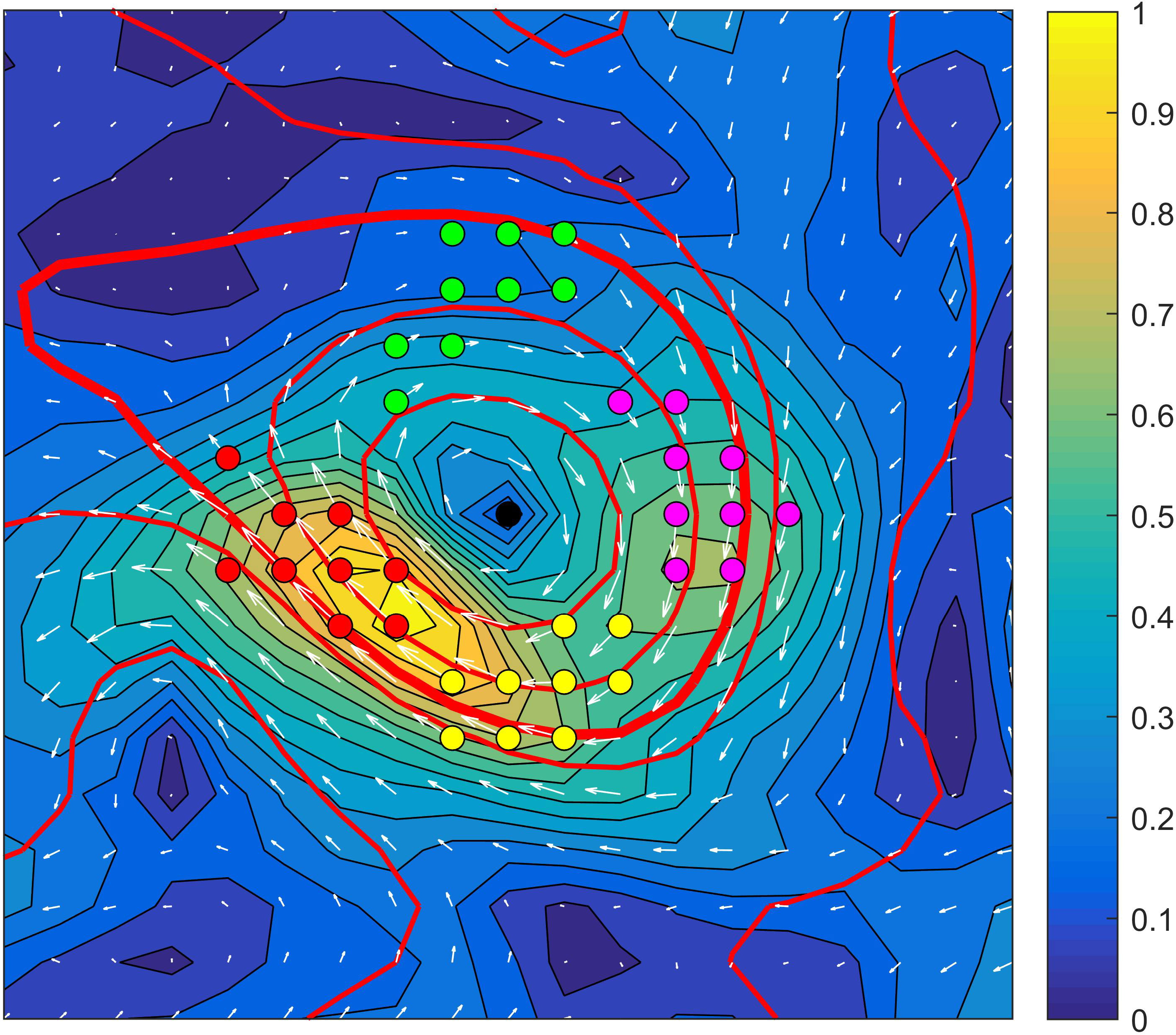
Figure 2 Four kinds of assimilation strategies. The colored bold points denote the (synthetic) observations and the red, green, purple, and yellow dots correspond to the (synthetic) observations assimilated by PF1, PF2, PF3, and PF4, respectively. The PF1 assimilates nine observations in the sensitive area, while the PF2, PF3, and PF4 assimilate nine observations in the non-sensitive area obtained by rotating 90°, 180°, and 270° along the vortex rotation direction starting from the PF1 assimilation area, respectively. Note that the distribution of the nine observations in each area shows an example of randomly selected 10 groups of observational locations.

The extent of the error reduction from assimilation is evaluated by Eq. (6).

$\begin{array}{ll}b=\frac{\text{d}{F}_1-\text{d}{F}_2}{\text{d}{F}_1}\times 100\%& (6)\end{array}$

where dF₁ is the forecast error of the Control Run with respect to the Truth Run and dF₂ is that of the Assimilation Run with respect to the Truth Run. It is noted that these forecast errors are both measured by the root mean square error (RMSE) with the formula as in Eq. (7).

$\begin{array}{ll}\text{RMSE}=\sqrt{\frac{1}{m}{\displaystyle \sum _{i=1}^m{(P_i-T_i)}^2}},& (7)\end{array}$

where m represents the total number of grid points in the concerned forecast area, and T_i P_i are the truth and its prediction on the ith grid point, respectively.

4 Evaluation of the sensitivity on the mesoscale eddy

In this section, we evaluate the sensitivity on mesoscale eddies of SSHA forecasting by using the realistic oceanic data provided in Section 2; particularly, we focus on the KE region and separate the circulation fields of strong and weak dynamical instabilities to do it.

4.1 The validity of the sensitivity on mesoscale eddy in promoting the SSHA forecasting skill

The assimilation strategies shown in Figure 2 are implemented to the Control Run of each Truth Run, and the extent of the error reduction from assimilation, i.e., b in Eq. (6), is calculated. Figure 3 shows the box plots of b for the three sets of SSHA data over the KE region, where the values of b are relative to the selected eddies and the randomly selected 10 groups of observations in each area on the eddies (see Section 3). It is easily seen that, for all the three datasets, the values of b in PF1 are always obviously larger than those in PF2, PF3, and PF4. Furthermore, when we examine respectively the three datasets to count the number of eddies that exhibit the largest value of b among the PF1, PF2, PF3, and PF4 strategies in terms of the ensemble mean after assimilating 10 groups of observations, we find that the number of eddies using the PF1 assimilation strategy is the highest (see Table 1). This indicates that the PF1 strategy, for the collected eddies, has a larger probability to significantly enhance the corresponding SSHA forecasting skill, as compared with the PF2/3/4 strategies. This result, combined with the sensitivity on the accuracy of the mesoscale eddy revealed by Jiang et al. (2022), shows that PF1 could be the optimal assimilation strategy for SSHA forecasting. This implies that additional observations should be preferentially implemented in the areas with a clear high- to low-velocity gradient along the rotation direction on mesoscale eddies. Consequently, the sensitive area of the mesoscale eddy associated with SSHA forecasting determined by CNOP is effective even when using more realistic marine data including model data, reanalysis, and observations. This also sheds light on that the sensitive area identified by the conceptual QG model in Jiang et al. (2022) could be robust, which therefore could provide reliable scientific guidance for implementing additional observations of actual mesoscale eddies in realistic field campaigns for improving SSHA forecasting skill.

FIGURE 3

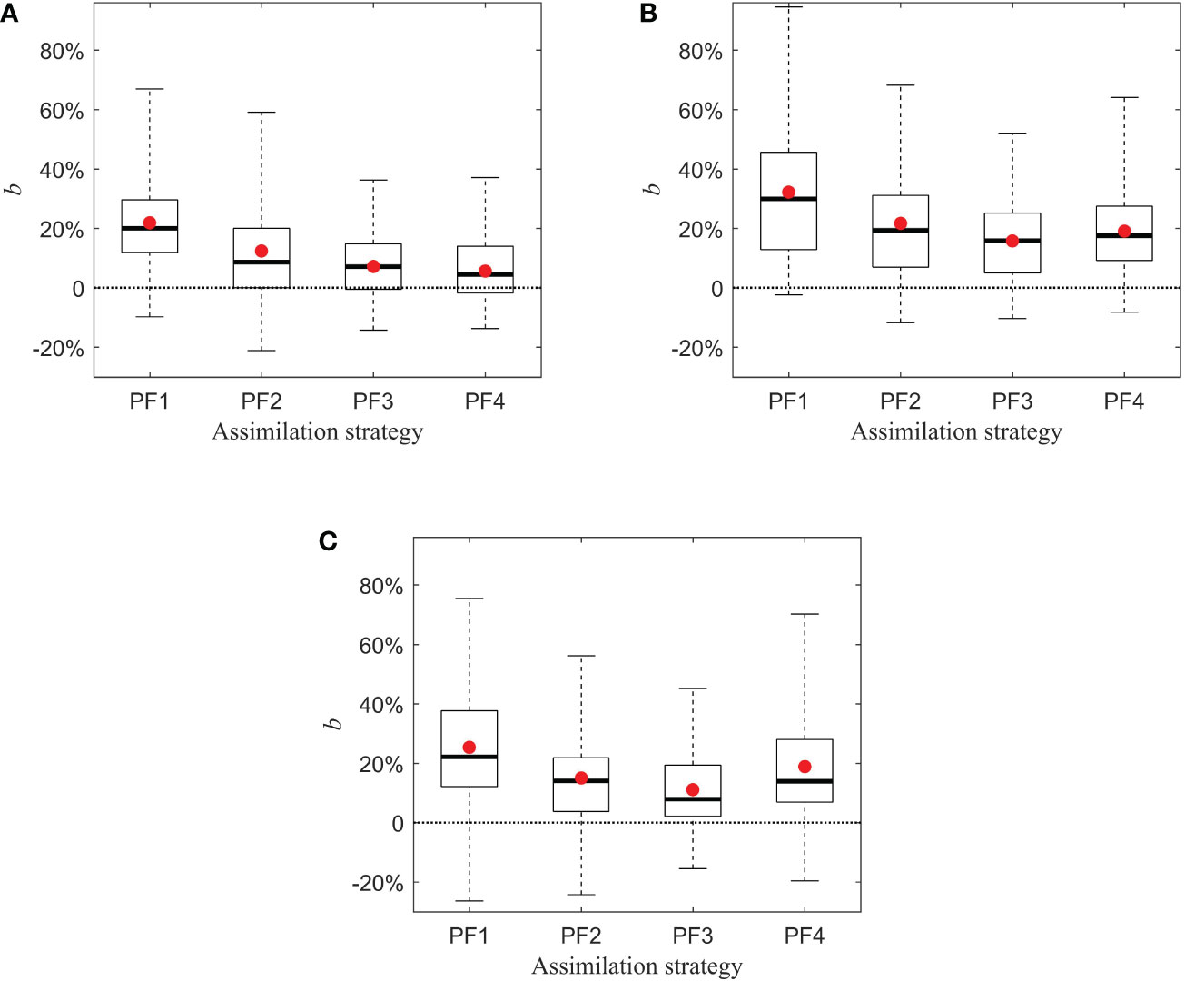
Figure 3 The box plots of b for the PF1, PF2, PF3, and PF4 assimilation strategies using (A) LICOM3 data, (B) GLORYS2V4 data, and (C) AVISO data, with respect to selected eddies and 10 groups of observations for each area.

TABLE 1

Table 1 The numbers of eddies with the largest value of b occurring in PF1, PF2, PF3, and PF4, respectively.

4.2 Modulating effect of ocean circulation instability on the sensitivity on mesoscale eddies

We have verified that the PF1 assimilation strategy of the sensitive areas of mesoscale eddies is superior to the PF2/3/4 strategies of non-sensitive areas for improving the SSHA forecasting skill. It is noted that we are concerned about the mesoscale eddies over the KE region. Meanwhile, it is known that there exist baroclinic (BC) and/or barotropic (BT) instabilities of ocean circulation in the KE region in the presence of strong shear of the eastward-flowing jet; furthermore, notable differences in instability strengths exist between the upstream and downstream KE regions with the former having much stronger instability (Spall, 2000; Williams et al., 2007; Stammer et al., 2012; Bishop, 2013). Then how will these instabilities affect the sensitivity on mesoscale eddies? To address this question, we will separate the upstream and downstream regions of the KE and further analyze the sensitivity on mesoscale eddies.

Referring to Yang and Liang (2016), we recognize the regions west of 154°E as the upstream region and the east of 154°E as the downstream region. Then, there are 40/15, 20/21, and 30/25 eddies in the upstream/downstream KE regions from LICOM3 data, GLORYS2V4 data, and AVISO data, respectively. For these eddies, we investigate the sensitivity on mesoscale eddies of the SSHA forecasting using the assimilation strategies as in Section 3 and identify the differences between the upstream and downstream regions.

The results are plotted in Figure 4 and Table 2. Obviously, all of the three datasets demonstrate that the value of b is still the largest when using the PF1 strategy in either upstream or downstream regions, and the number of eddies with PF1 being the most effective assimilation strategy is also the largest (see Table 2). This indicates that the advantages of the PF1 strategy are still valid over both upstream and downstream regions. When we further compare the degrees of improvements of the SSHA forecasting skill due to assimilation between upstream and downstream, it seems that PF1 provides an improvement in the upstream KE region with almost the same degree as in the downstream region, according to the arithmetic mean and median of improvements; however, when we count the number of eddies that possess the largest value of b in PF1, PF2, PF3, and PF4, it is found that the percentage of the number of eddies with PF1 being the best assimilation strategy to the total number of eddies in the upstream region is obviously larger than that in the downstream region (see Table 2). Obviously, this indicates that assimilating additional observations located in sensitive areas of mesoscale eddies in the upstream region, compared with doing it in the downstream region, possesses a greater probability to improve the corresponding SSHA forecasting skill, although the improvements in these two regions are of less different amplitudes.

FIGURE 4

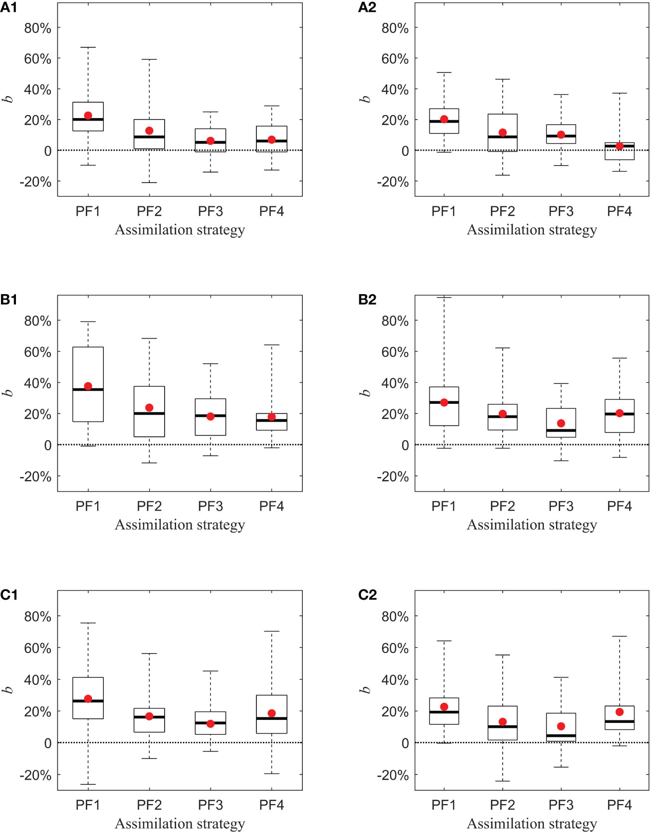
Figure 4 The box plots of b of PF1, PF2, PF3, and PF4 in the upstream (1) and downstream (2) of the KE, with respect to selected eddies and 10 groups of observations for each area. (A–C) For the LICOM model data, GLORYS2V4 data, and AVISO data, respectively.

TABLE 2

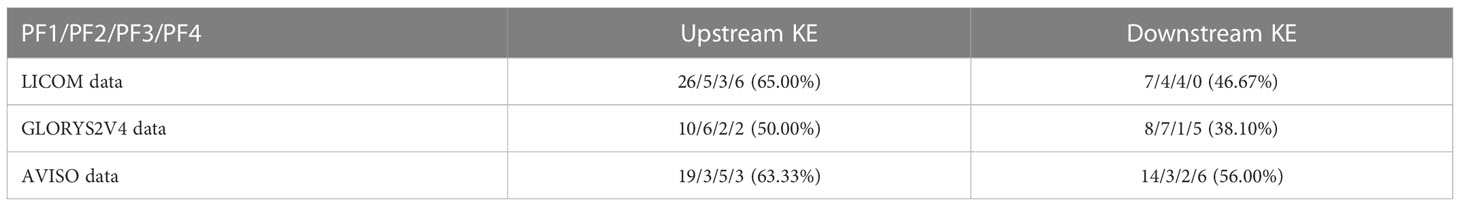
Table 2 The number of eddies with the largest value of b in PF1/PF2/PF3/PF4 and the percentages of the number of eddies with the largest value of b in the PF1 to the total eddy number in the upstream and downstream KE regions.

To sum up, it is particularly noteworthy that, for more realistic ocean data of LICOM3 data, GLORYS2V4 data, and AVISO data investigated here, the assimilation implemented in the sensitive area of mesoscale eddies in the upstream region exhibits more advantages than that conducted in the downstream region to improve the SSHA forecasting skill. Therefore, the sensitivity on mesoscale eddies of the SSHA forecasting is more prominent in the upstream KE region than in the downstream region, and it is more effective for improving the SSHA forecasting level to assimilate additional observations located in the sensitive areas of mesoscale eddies in the upstream KE region.

4.3 Interpretation

In this section, we would interpret why the SSHA forecasting skill is more prominently improved in the upstream KE region than in the downstream KE region by preferentially implementing the additional assimilation in the sensitive area of mesoscale eddies. In fact, this conclusion involves the energy conversion of different spatial scales. Results in previous studies have shown that mesoscale eddies tend to extract energy from mean flow (ocean circulation) in the upstream KE region along the stream direction through an eddy–wave interaction, but they are inclined to transmit energy to mean flow in the downstream KE region (Hall, 1991; Yang and Liang, 2018). Therefore, the stronger BT or BC instability in the upstream KE region would induce a stronger eddy–wave interaction and make the circulation mean flow transmit more energies to the mesoscale eddies; as such, the mesoscale eddies in the upstream KE region possess more energies. Then, on mesoscale eddies, the initial perturbations located in the sensitive area, where a clear high- to low-velocity gradient along the eddy rotation is presented, would stimulate a much larger positive BT conversion rate according to the equation $\text{BT}=-\frac{V{\text{'}}^2}{(\overline{V}+V\text{'})}·\frac{\partial \overline{V}}{\partial t}$ with the negative velocity tendency $\frac{\partial \overline{V}}{\partial t}<0$ due to a high- to low-velocity gradient in the sensitive area, where V’ is the velocity component of the initial perturbations and $\overline{V}$ represents the flow velocity of the mesoscale eddy in a natural coordinate system [the details are referred to as in Jiang et al. (2022)]. Consequently, the energies transmitted from the mean flow to the mesoscale eddies in the upstream KE region would be provided much more to the perturbation and would enhance its much quicker growth, finally yielding a much greater impact on the SSHA forecasting in the upstream KE region. That is to say, the SSHA forecasting in the upstream region is much more sensitive to the accuracy of the mesoscale eddies there, especially sensitive to the accuracy of the flow field in the sensitive area of mesoscale eddies. Then, if we give priority to implementing additional observations in the sensitive area of mesoscale eddies in the upstream KE region and assimilate them to the Control Run for improving its initial field, the SSHA forecasting skill would have more probabilities to achieve much greater improvement. On the contrary, for the downstream KE region with much weaker BT or BC instability, the energies transmitted from the ocean circulation to the mesoscale eddies are much less, and thus, there are not enough energies provided to promote the growth of the initial perturbations even in the sensitive areas of mesoscale eddies, eventually exerting a weaker impact on the SSHA forecasting there. Therefore, the sensitivity on mesoscale eddies in the downstream region of weaker instability is not as strong as that in the upstream region of stronger instability, and assimilating additional observations in the sensitive areas in the downstream region to the Control Run is certainly less effective than doing it in the upstream region for improving the SSHA forecasting skill.

Combining the above numerical results and theoretical reasoning, it is concluded that the stronger the dynamical instability of mean flow (or ocean circulation), the stronger the sensitivity on mesoscale eddies of SSHA forecasting. Therefore, in the regions with a strong instability of ocean circulation, such as in upstream KE, more attention should be preferentially paid to assimilating additional observations (i.e., the targeted observations) on mesoscale eddies, so as to efficiently improve the accuracy of mesoscale eddies and, thus, greatly increase the SSHA forecasting skill.

5 Conclusion and discussion

In this paper, the sensitivity on mesoscale eddies of SSHA forecasting, determined by CNOP through a conceptual QG model (Jiang et al., 2022), is further evaluated using three sets of realistic marine data, particularly including the LICOM3 model data, GLORYS2V4 reanalysis data, and AVISO altimeter observation data. An advanced PF assimilation method is implemented over the KE region to improve the initial accuracy of mesoscale eddies there and then increase the corresponding SSHA forecasting. Four assimilation strategies are tested, which are relevant with the assimilation in the sensitive area, where a clear high- to low-velocity gradient along the eddy rotation is presented, and those in the other three non-sensitive areas of mesoscale eddies. The results demonstrate that the assimilation implemented in the sensitive area of mesoscale eddies is most effective for promoting the SSHA forecasting skill. This sheds light on the fact that the sensitivity on mesoscale eddy of SSHA forecasting determined by the QG model together with the CNOP approach in Jiang et al. (2022) is reasonable even in realistic marine data. It is therefore concluded that the sensitivity on mesoscale eddies obtained by the QG model is reliable for providing scientific guidance for targeting observation of actual mesoscale eddies associated with SSHA forecasting in the KE region. That is to say, additional observations in the sensitive areas of mesoscale eddies should be preferentially implemented and/or assimilated in order to greatly improve the forecasting skills of SSHA in the KE region.

The above sensitivity on mesoscale eddies is also tested by separating the upstream and downstream regions of KE. The upstream region presents the oceanic circulation with much stronger dynamical (BT and/or BC) instability, while the downstream region provides much weaker instability. It is shown that the assimilation implemented in the sensitive areas of mesoscale eddies in the upstream region has more probabilities than that in the downstream region for improving the SSHA forecasting skill. Theoretically, the stronger eddy–wave interaction induced by the stronger instability in the upstream KE region tends to make the ocean circulation transmit more energies to the mesoscale eddies there, thus being favorable for more energies further provided to the disturbances on the eddies through the mechanism of the BT instability [see Jiang et al. (2022)] and finally yielding a much greater impact on the SSHA forecasting in the upstream KE region due to the growth of disturbances, and the strongest instability in the sensitive area of mesoscale eddies would enhance most the growth of the disturbances of the SSHA. It is therefore certain that, if additional observations are preferentially implemented in the sensitive area in the upstream KE region and assimilated to the model fields, the growth of initial errors there would be greatly suppressed and the corresponding SSHA forecasting skill would be much more significantly improved. It is suggested that more attention should be preferentially paid to the assimilation of the targeted observations on mesoscale eddies located in the area where the background ocean circulation presents stronger instability, such as the upstream KE region, in order to efficiently improve the SSHA forecasting skill.

The sensitivity on mesoscale eddies of SSHA prediction was revealed in Jiang et al. (2022) and in the present study, and it is further practically evaluated through three sets of realistic ocean data; moreover, more concerns are additionally suggested to the sensitivity on mesoscale eddies over the upstream region for improving the SSHA forecasting skill there. However, due to the limitation of the offline data adopted in the present study, we have to deduce the possible dynamical mechanism responsible for the relationship between the sensitivity on mesoscale eddy and the dynamical instability of the background mean flow; therefore, a quantitative evaluation is expected to verify the dynamics of the modulation role of the mean flow to the sensitivity on mesoscale eddy of the SSHA forecasts by using specific ocean models, such as the Regional Ocean Modeling System. Also, the PF assimilation method used in this paper has the advantages of easy operation and offline implementation, whereas the phenomenon of particle degeneracy sometimes occurs and severely influences the quality of assimilating results; as such, other data assimilation methods, such as the ensemble Kalman filter and four-dimensional variational methods, are anticipated to be applied in specific models to examine the sensitivity on mesoscale eddies of the SSHA predictions. Doing such would also help investigate the sensitivity on mesoscale eddies from the three-dimensional structure on mesoscale eddy, rather than from the frame of two-dimensional motion of mesoscale eddy in the present study. The interactions among eddies would induce anomalies of ocean state and play a significant effect on the underlying atmosphere, such as winds, clouds, precipitation, and typhoons (Chelton, 2013; Renault et al., 2019) by the air–sea interaction, and thus, relevant studies are also expected. The present study focuses on the accuracy of mesoscale eddies but is related to the forecast of SSHA. In fact, the predictions of mesoscale eddy and its moving track and intensity are essential for describing further ocean state and its underlying atmosphere, and therefore, the corresponding predictability study should be carried out comprehensively although it is much more challenging. It is expected that the present study and the associated study of Jiang et al. (2022) can provide useful ideas to address the predictability of mesoscale eddies themselves.

Data availability statement

The raw data supporting the conclusions of this article will be made available upon reasonable request and with authors’permission. Open source datasets include the GLORYS2V4 data and AVISO data (both available online at https://resources.marine.copernicus.eu.).

Author contributions

LJ and WD conceived the research, designed the experiments, performed the simulations, and analyzed the results. All authors contributed to the article and approved the submitted version.

Funding

The study was supported by the National Natural Science Foundation of China (Grant No. 41930971).

Conflict of interest

The authors declare that the research was conducted in the absence of any commercial or financial relationships that could be construed as a potential conflict of interest.

Publisher’s note

All claims expressed in this article are solely those of the authors and do not necessarily represent those of their affiliated organizations, or those of the publisher, the editors and the reviewers. Any product that may be evaluated in this article, or claim that may be made by its manufacturer, is not guaranteed or endorsed by the publisher.

References

Agarwal N., Sharma R., Kumar R. (2022). Impact of along-track altimeter sea surface height anomaly assimilation on surface and sub-surface currents in the bay of Bengal. Ocean Model. 169 (9),101931. doi: 10.1016/j.ocemod.2021.101931

CrossRef Full Text | Google Scholar

Bishop S. P. (2013). Divergent eddy heat fluxes in the kuroshio extension at 144°–148°E. part II: Spatiotemporal variability. J. Phys. Oceanogr. 43 (11), 2416–2431. doi: 10.1175/jpo-d-13-061.1

CrossRef Full Text | Google Scholar

Chelton D. (2013). Mesoscale eddy effects. Nat. Geosci. 6 (8), 594–595. doi: 10.1038/ngeo1906

CrossRef Full Text | Google Scholar

Chelton D. B., Schlax M. G., Samelson R. M. (2011). Global observations of nonlinear mesoscale eddies. Prog. Oceanogr. 91 (2), 167–216. doi: 10.1016/j.pocean.2011.01.002

CrossRef Full Text | Google Scholar

Duan W. S., Feng F. (2018). Application of particle filter assimilation in the target observation for El niño–southern oscillation. Chin. J. Atmos. Sci. (in Chinese) 42 (3), 677–695. doi: 10.3878/j.issn.1006-9895.1711.17264

CrossRef Full Text | Google Scholar

Duan W. S., Yang L. C., Mu M., Wang B., Shen X. S., Meng Z. Y., et al. (2022). Advances in predictability study on weather and climate in China. Adv. Atmos. Sci. in reviewing.

Google Scholar

Fang M. (2006). Study of assimilating the satellite Sea surface temperature and Sea surface height anomaly into an East China Sea model - a progress report. 2nd Dragon Symposium, Santorini, Greece. European Space Agency Publications Division.

Google Scholar

Ferrari R., Wunsch C. (2009). Ocean circulation kinetic energy: Reservoirs, sources, and sinks. Annu. Rev. Fluid Mech. 41 (1), 253–282. doi: 10.1146/annurev.fluid.40.111406.102139

CrossRef Full Text | Google Scholar

Ferry N., Parent L., Garric G., Barnier B., Jourdain N. (2010). Mercator Global eddy permitting, ocean reanalysis GLORYS1V1: Description and results. Mercator-Ocean Q. Newslett. 36, 15–27.

Google Scholar

Fraser R., Palmer M., Roberts C., Wilson C., Copsey D., Zanna L. (2019). Investigating the predictability of north Atlantic sea surface height. Climate Dyn. 53 (3-4), 2175–2195. doi: 10.1007/s00382-019-04814-0

CrossRef Full Text | Google Scholar

Hall M. M. (1991). Energetics ot the kuroshio extension at 35°N,152°E. J. Phys. Oceanogr. 21, 958–975. doi: 10.1175/1520-0485(1991)0210958:EOTKEA>2.0.CO;2

CrossRef Full Text | Google Scholar

Hou M., Tang Y., Duan W., Shen Z. (2022). Toward an optimal observational array for improving two flavors of El niño predictions in the whole pacific. Climate Dyn. doi: 10.1007/s00382-022-06342-w

CrossRef Full Text | Google Scholar

Jiang L., Duan W., Liu H. (2022). The most sensitive initial error of Sea surface height anomaly forecasts and its implication for target observations of mesoscale eddies. J. Phys. Oceanogr. 52, 723–740. doi: 10.1175/jpo-d-21-0200.1

CrossRef Full Text | Google Scholar

Kramer W., Dijkstra H. A. (2013). Optimal localized observations for advancing beyond the ENSO predictability barrier. Nonlinear Process. Geophys. 20 (2), 221–230. doi: 10.5194/npg-20-221-2013

CrossRef Full Text | Google Scholar

Lellouche J., Greiner E., Galloudec O., Garric G., Regnier C., Drevillon M., et al. (2018). Recent updates to the Copernicus marine service global ocean monitoring and forecasting real-time 1/12° high-resolution system. Ocean Sci. 14, 1093–1126. doi: 10.5194/os-14-1093-2018

CrossRef Full Text | Google Scholar

Li Y., Liu H., Ding M., Lin P., Yu Z., Yu Y., et al. (2020). Eddy-resolving simulation of CAS-LICOM3 for phase 2 of the ocean model intercomparison project. Adv. Atmos. Sci. 37 (10), 1067–1080. doi: 10.1007/s00376-020-0057-z

CrossRef Full Text | Google Scholar

Li X., Zhu J., Xiao Y., Wang R. (2010). A model-based observation-thinning scheme for the assimilation of high-resolution SST in the shelf and coastal seas around China. J. Atmos. Ocean. Technol. 27, 1044–1058. doi: 10.1175/2010jtecho709.1

CrossRef Full Text | Google Scholar

Lumban-Gaol J., Leben R. R., Vignudelli S., Mahapatra K., Okada Y., Nababan B., et al. (2017). Variability of satellite-derived sea surface height anomaly, and its relationship with bigeye tuna (Thunnus obesus) catch in the Eastern Indian ocean. Eur. J. Remote Sens. 48 (1), 465–477. doi: 10.5721/EuJRS20154826

CrossRef Full Text | Google Scholar

Moradkhani H., Hsu K.-L., Gupta H., Sorooshian S. (2005). Uncertainty assessment of hydrologic model states and parameters: Sequential data assimilation using the particle filter. Water Resour. Res. 41 (5), W05012. doi: 10.1029/2004wr003604

CrossRef Full Text | Google Scholar

Mu M., Duan W. S., Wang B. (2003). Conditional nonlinear optimal perturbation and its applications. Nonlinear Process. Geophys. 10 (6), 493–501. doi: 10.5194/npg-10-493-2003

CrossRef Full Text | Google Scholar

Nakamura H., Isobe A., Minobe S., Mitsudera H., Nonaka M., Suga T. (2015). “Hot spots” in the climate system–new developments in the extratropical ocean–atmosphere interaction research: a short review and an introduction. J. Oceanogr. 71 (5), 463–467. doi: 10.1007/s10872-015-0321-5

CrossRef Full Text | Google Scholar

Parent L., Ferry N., Garric G., Legalloudec O., Testut C.-e., Barnier B., et al. (2011). GLORYS2: A global ocean reanalysis simulation of the period 1992-present. 13. Abstract retrieved from Abstracts in Geophysical Research Abstracts.

Google Scholar

Qiu B., Chen S. (2005). Variability of the kuroshio extension jet, recirculation gyre, and mesoscale eddies on decadal time scales. J. Phys. Oceanogr. 35 (11), 2090–2103. doi: 10.1175/jpo2807.1

CrossRef Full Text | Google Scholar

Renault L., Masson S., Oerder V., Jullien S., Colas F. (2019). Disentangling the mesoscale ocean-atmosphere interactions. J. Geophys. Res.: Oceans 124 (3), 2164–2178. doi: 10.1029/2018jc014628

CrossRef Full Text | Google Scholar

Snyder C. (1996). Summary of an informal workshop on adaptive observations and FASTEX. Bull. Am. Meteorol. Soc. 77, 953–961. doi: 10.1175/1520-0477-77.5.953

CrossRef Full Text | Google Scholar

Solanki H. U., Bhatpuria D., Chauhan P. (2015). Signature analysis of satellite derived SSHa, SST and chlorophyll concentration and their linkage with marine fishery resources. J. Mar. Syst. 150, 12–21. doi: 10.1016/j.jmarsys.2015.05.004

CrossRef Full Text | Google Scholar

Song T., Han N., Zhu Y., Li Z., Li Y., Li S., et al. (2021). Application of deep learning technique to the sea surface height prediction in the south China Sea. Acta Oceanol. Sin. 40 (7), 68–76. doi: 10.1007/s13131-021-1735-0

CrossRef Full Text | Google Scholar

Spall M. A. (2000). Generation of strong mesoscale eddies by weak ocean gyres. J. Mar. Res. 58 (1), 97–116. doi: 10.1357/002224000321511214

CrossRef Full Text | Google Scholar

Stammer D., Marotzke J., Maier-Reimer E., Hernández-Deckers D., Haak H., Fast I., et al. (2012). An estimate of the Lorenz energy cycle for the world ocean based on the STORM/NCEP simulation. J. Phys. Oceanogr. 42 (12), 2185–2205. doi: 10.1175/jpo-d-12-079.1

CrossRef Full Text | Google Scholar

Tanajura C. A. S., Lima L. N., Belyaev K. P. (2015). Assimilation of satellite surface-height anomalies data into a hybrid coordinate ocean model (HYCOM) over the Atlantic ocean. Oceanology 55 (5), 667–678. doi: 10.1134/s0001437015050161

CrossRef Full Text | Google Scholar

Tanajura C. A. S., Lima L. N., Belyaev K. (2016). Impact on oceanic dynamics from assimilation of satellite surface height anomaly data into the hybrid coordinate ocean model ocean model (HYCOM) over the Atlantic ocean. Oceanology 56 (4), 509–514. doi: 10.1134/s000143701603022x

CrossRef Full Text | Google Scholar

Tandeo P., Chapron B., Ba S., Autret E., Fablet R. (2014). Segmentation of mesoscale ocean surface dynamics using satellite SST and SSH observations. IEEE Trans. Geosci. Remote Sens. 52 (7), 4227–4235. doi: 10.1109/tgrs.2013.2280494

CrossRef Full Text | Google Scholar

Tang Q., Gulick S. P. S., Sun J., Sun L., Jing Z. (2020). Submesoscale features and turbulent mixing of an oblique anticyclonic eddy in the gulf of Alaska investigated by marine seismic survey data. J. Geophys. Res.: Oceans 125 (1). doi: 10.1029/2019jc015393

CrossRef Full Text | Google Scholar

Tsujino H., Urakawa S., Nakano H., Small R., Kim W., Yeager S., et al. (2018). JRA-55 based surface dataset for driving ocean-sea-ice models (JRA55-do). Ocean Model. 130, 79–139. doi: 10.1016/j.ocemod.2018.07.002

CrossRef Full Text | Google Scholar

Waterman S., Hogg N. G., Jayne S. R. (2011). Eddy–mean flow interaction in the kuroshio extension region. J. Phys. Oceanogr. 41 (6), 1182–1208. doi: 10.1175/2010jpo4564.1

CrossRef Full Text | Google Scholar

Weiss J. B., Grooms I. (2017). Assimilation of ocean sea-surface height observations of mesoscale eddies. Chaos 27 (12), 126803. doi: 10.1063/1.4986088

PubMed Abstract | CrossRef Full Text | Google Scholar

Williams R. G., Wilson C., Hughes C. W. (2007). Ocean and atmosphere storm tracks: The role of eddy vorticity forcing. J. Phys. Oceanogr. 37 (9), 2267–2289. doi: 10.1175/jpo3120.1

CrossRef Full Text | Google Scholar

Wyrtki K., Magaard L., Hager J. (1976). Eddy energy in the oceans. J. Geophys. Res. 81 (15), 2641–2646. doi: 10.1029/JC081i015p02641

CrossRef Full Text | Google Scholar

Xie X., Verbraeck A. (2018). A particle filter-based data assimilation framework for discrete event simulations. Simulation 95 (11), 1027–1053. doi: 10.1177/0037549718798466

CrossRef Full Text | Google Scholar

Yang Y., Liang X. S. (2016). The instabilities and multiscale energetics underlying the mean–Interannual–Eddy interactions in the kuroshio extension region. J. Phys. Oceanogr. 46 (5), 1477–1494. doi: 10.1175/jpo-d-15-0226.1

CrossRef Full Text | Google Scholar

Yang Y., Liang X. S. (2018). On the seasonal eddy variability in the kuroshio extension. J. Phys. Oceanogr. 48 (8), 1675–1689. doi: 10.1175/jpo-d-18-0058.1

CrossRef Full Text | Google Scholar

Yavuzdoğan A., Tanır Kayıkçı E. (2020). A copula approach for sea level anomaly prediction: a case study for the black Sea. Surv. Rev. 53 (380), 436–446. doi: 10.1080/00396265.2020.1816314

CrossRef Full Text | Google Scholar

Zanna L., Brankart J. M., Huber M., Leroux S., Penduff T., Williams P. D. (2018). Uncertainty and scale interactions in ocean ensembles: From seasonal forecasts to multidecadal climate predictions. Q. J. R. Meteorol. Soc. 145 (S1), 160–175. doi: 10.1002/qj.3397

CrossRef Full Text | Google Scholar