The second-generation real-time ecological environment prediction system for the Guangdong–Hong Kong–Marco Greater Bay Area: Model setup, validation, improvements, and online visualization

With the rapidly growing population and socioeconomic development of the Guangdong–Hong Kong–Marco Greater Bay Area of China, inputs of diverse contaminants have rapidly increased. This poses threats to the water quality of the Pearl River Estuary (PRE) and adjacent seas. To provide valuable information to assist the governors, stakeholders, and decision-makers in tracking changes in environmental conditions, daily nowcasts and two-day forecasts from the ecological prediction system, namely the Coupled Great Bay Ecological Environmental Prediction System (CGEEPS), has been setup. These forecast systems have been built on the Coupled Ocean–Atmosphere–Wave–Sediment Transport modelling system. This comprises an atmospheric Weather Research Forecasting module and an oceanic Regional Ocean Modelling System module. Daily real-time nowcasts and 2-day forecasts of temperature, salinity, NO2 + NO3, chlorophyll, and pH are continuously available. Visualizations of the forecasts are available on a local website (http://www.gbaycarbontest.xyz:8008/). This paper describes the setup of the environmental forecasting system, evaluates model hindcast simulations from 2014 to 2018, and investigates downscaling and two-way coupling with the regional atmospheric model. The results shown that though CGEEPS lacks accuracy in predicting the absolute value for biological and biogeochemical environmental variables. It is quite informative to predict the spatio-temporal variability of ecological environmental changes associated with extreme weather events. Our study will benefit of developing real-time marine biogeochemical and ecosystem forecast tool for oceanic regions heavily impact by extreme weathers.

1 Introduction

The Pearl River Estuary (PRE) in South China is a large subtropical permanent open estuary fed by the Pearl River, which is the second largest river in China in terms of freshwater discharge (3.3 × 10¹¹ m³/yr) (Figure 1). Due to the substantial amount of anthropogenic nutrient inputs along with high discharge, the PRE is relatively productive with a high level of biodiversity. It provides crucial habitat and natural resources for multiple marine and freshwater fish species and the Chinese white dolphin, which is designated as a first-class national protected animal (Jefferson and Hung, 2004; Zhou et al., 2019). Oyster aquaculture has also developed rapidly in the PRE since the Ming and Qing dynasties, generating high revenue for the Guangdong government (Liu and Song, 2022). According to Cai and Li (2011), the PRE marine ecosystem is estimated to be valued at $31 billion per year. This represents an important component of the Gross Domestic Product of the Guangdong–Hong Kong–Marco Greater Bay Area.

FIGURE 1

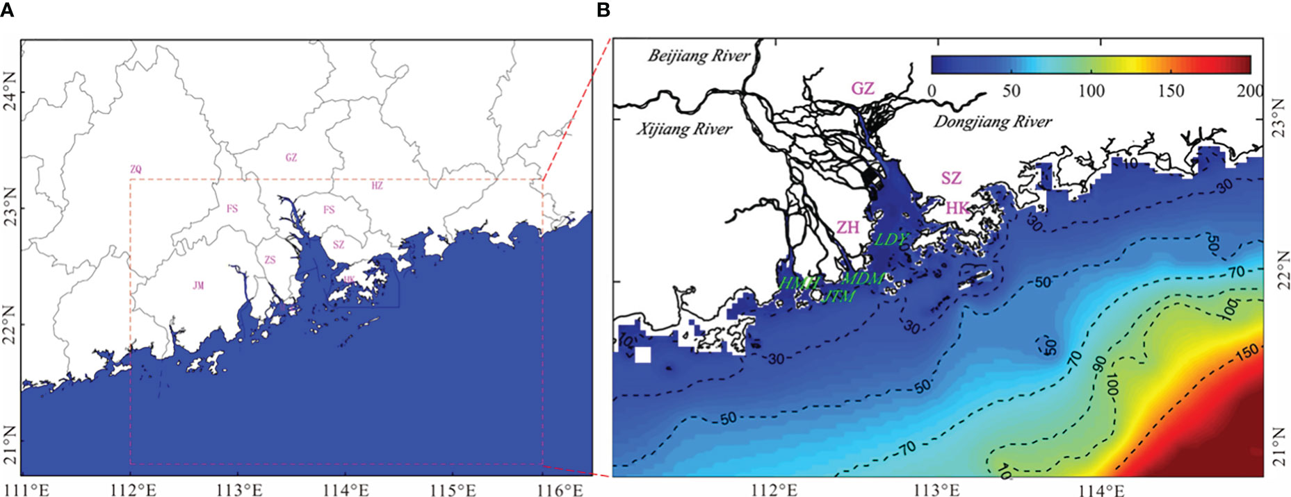
Figure 1 (A) Cites of Guangdong–Hong Kong–Marco Greater Bay Area, including Zhao-Qing (ZQ), Guang-Zhou (GZ), Hui-Zhou (HZ), Fo-Shan (FS), Dong-Guan (DG), Jiang-Men (JM), Zhong-Shan (ZS), Shen-Zhen (SZ), Zhu-Hai (ZH), Macau (MC), and Hong Kong (HK). (B) The tributaries of Pearl River, the Pearl River Estuary (PRE) and adjacent seas. Abbreviations are sub estuaries, including Ling-Ding-Yang (LDY), Mo-Dao-Men (MDM), Huang-Mao-Hai (HMH), and Ji-Ti-Men (JTM).

Over the last few decades, rapid economic growth and progressive urbanization in the Pearl River Delta have led to considerable population growth in large cities in this region, including Hong Kong, Macao, Shenzhen, Zhuhai, and Guangzhou. This population increase poses a threat to the water quality of the PRE due to dumping of new pollutants, such as organophosphorus compounds, pharmaceuticals, and microplastics derived from personal care products (Stedman and Dahl, 2008; Zhou et al., 2016; Wang and Rainbow, 2020). These pollutants can cause severe damage to estuarine ecosystems and reduce biodiversity and fishery resources. This has caused substantial ecological and economic losses. Thus far, the loss value of the PRE is estimated to be approximately $5 billion per year. Therefore, protecting the estuarine environment from further water quality degradation is of considerable interest to stakeholders.

Real-time environmental forecasting systems based on three-dimensional, coupled hydrodynamic-biogeochemistry models are important tools for providing information on spatio-temporal varied environmental conditions (Wang, 2001). These data can be used to assist local governments and private partners to establish specific strategies for water quality improvement. The increase in anthropogenic derived nutrients has fueled larger and more frequent hypoxia in recent years (Li D et al., 2020; Ma et al., 2009; Ye et al., 2017; Qian et al., 2018). Oyster aquaculture has been shown to mitigate eutrophication and hypoxia, whereas the location and size of the farming area require circulation and appropriate biogeochemical conditions (Yu and Gan, 2021).

The coupled hydrodynamic–biogeochemical model usually serves as the internal core of a real-time environmental forecasting system. Web-based visualization systems are another important component that aid in forecasting. Real-time environmental systems with visualization systems can provide an intuitive way for governments and private partners to understand data and facilitate rapid decision-making. These systems have been established in many estuarine areas and oceans adjacent to coastal areas worldwide. For example, the Chesapeake Bay Environmental Forecast System(CBEFS) runs every 6 h over 1–2 km as well as the Chesapeake Bay Regional Ocean Modelling System (ChesROMS) – Estuarine Carbon Biogeochemistry (ECB) Model (Feng et al., 2015). CBEFS can provide real-time nowcast and two-day forecasts of salinity, water temperature, pH, aragonite saturation state, alkalinity, dissolved oxygen, and hypoxic volume in graphics on the local website (www.vims.edu/hypoxia). Another example of a real-time forecasting system is the China high-resolution coastal ocean ecological environment numerical prediction system. This was constructed using the Regional Ocean Modelling System–Carbon Silicate and Nitrogen Ecosystem model (ROMS-CoSiNE) and Semi-implicit Cross-scale Hydroscience-Integrated System Model-CoSiNE (SCHIMS-CoSiNE) for the BoHuang Sea, Yellow Sea, South China Sea, and Xiamen Bay (http://202.108.199.24:8080/BJ_SZYB_Web/default.html). The system can predict water temperature, current, multiple inorganic nutrients, chlorophyll, dissolved oxygen (DO), and pH predictions every 6 h. For the PRE, we constructed the Guangdong–Hong Kong–Marco Greater Bay Area Ecological Security Prediction System V1.0 using the Regional Ocean Modelling System (ROMS), Soil and Water Assessment Tool (SWAT), and Estuarine Carbon Biogeochemistry Model (ECB). The system was run every 24 h and primarily used for forecasting ocean currents, temperature, salinity, NO₂ + NO₃, chlorophyll, and DO (http://zhujiangtest.xyz:8000/).

This study describes an updated version of the real-time Ecological Environmental Forecast System for the Pearl River Estuary, the Coupled Great Bay Ecological Environment Prediction System (CGEEPS). We have introduced a general model configuration and evaluated the model accuracy for multiple hindcast variables and graphic visualization. CGEEPS provides daily nowcasts and two-day forecasts of environmental conditions throughout the PRE for temperature, salinity, NO₂ + NO₃, chlorophyll, DO, and pH. Configuration of the first generation of CGEEPS used a coupled ocean circulation–atmosphere model with a nitrogen-based ocean biogeochemistry component. The river inputs were generated from the land surface model SWAT climatology. We have added a range of updates that build on the first generation model (http://zhujiangtest.xyz:8000/). This includes a carbonate chemistry module that has been previously implemented in an existing nitrogen-based biogeochemistry model. River discharge was updated in near real-time from the China National Water and Rain Information Center (http://xxfb.mwr.cn/) and snatched by the Python request module.

The remainder of this paper is organized as follows. Section 2 presents the configuration of the modelling system core for the Forecast System and the model validation methodology. Section 3 presents the model validation and advantages of coupling it with the atmospheric model in a typhoon passage case. Section 4 summarizes the results and discusses the disadvantages of the current version of the forecasting system and potential future techniques that can be implemented.

2 Materials and methods

2.1 Atmosphere–ocean circulation–carbon biogeochemistry model implementation

The physical model of CGEEPS is built on the Coupled Ocean–Atmosphere–Wave–Sediment Transport (COAWST) modelling system. This comprises an atmospheric Weather Research Forecasting (WRF) module and a ROMS (Warner et al., 2008; Warner et al., 2010). The WRF domain spans from 98 ° to 122 °E and from 16 °to 30°N with an average horizontal resolution of approximately 12 km. This encompasses the entire Pearl River Watershed and northern part of the South China Sea. The ROMS domain ranges from 105° to 121°E and from 16° to 26°N, covering the continental shelf of the North South China Sea (NSCS) and the PRE (Figure 2A). The horizontal grid spacing varies between 2.8 km and 40.7 km with an average resolution of approximately 4 km. The model has 30 vertical layers that follow the terrain with a higher resolution near the surface and bottom boundaries. The vertical s-coordinate function is based on that of Shchepetkin and McWilliams (2009). The physical model is configured to use the recursive MPDATA 3-D advection scheme for tracers, four-order horizontal advection of tracers, third-order upwind advection of momentum, and the Mellor and Yamada (1982) turbulence closure scheme for vertical mixing. A viscosity/diffusivity coefficient of 10^-5m²s^-1 was used for biharmonic horizontal mixing in the momentum and tracer equations. Based on the CFL criterion, which is one of the global stability conditions, the internal mode time step of the numerical integration was 900 s, while the external mode time step was 60 s.

FIGURE 2

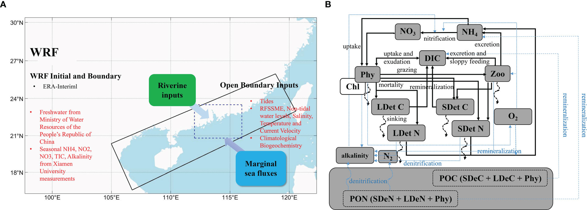
Figure 2 General setup of the Coupled Great Bay Ecological Environment Prediction System (CGEEPS) (A); the structure of the biogeochemistry model (B).

The circulation model was coupled with a nitrogen cycle model with consideration of carbonate chemistry and O₂ (Fennel et al., 2006, 2008, 2011). The model has 12 state variables, namely phytoplankton (Phy), chlorophyll (Chl), zooplankton (Zoo), nitrate (NO₃⁻), ammonium (NH₄⁺), O₂, dissolved inorganic carbon (DIC), total alkalinity (TAlk), and two detritus pools. These include small and large detritus, each split into nitrogen (SDetN and LDetN) and carbon (SDetC and LDetC) (Figure 2B). The mathematical description of the biogeochemical source and sink terms for the state variables is as follows.

$\begin{array}{ll}\frac{\partial \text{Phy}}{\partial t}={\mu }_{\text{max}}(T)f(E)L_{\text{N}}\text{Phy}-g_{\text{max}}\frac{{\text{Phy}}^2}{k_{\text{P}}+{\text{Phy}}^2}\text{Zoo}-m_{\text{P}}\text{Phy}- \tau (\text{SDetN}+\text{Phy})\text{Phy}-w_{\text{P}}\frac{\partial \text{Phy}}{\partial z} & (1)\end{array}$

Where

$\begin{array}{ll}{\mu }_{max}(T)={\mu }_0{1.066}^T& (2)\end{array}$

$\begin{array}{ll}f(E)=\frac{\alpha E}{\sqrt{{\mu }_{max}^2+{\alpha }^2{E}^2}}& (3)\end{array}$

$\begin{array}{ll}{L}_{N{O}_3}=\frac{N{O}_3}{k_{N{O}_3}+N{O}_3}\frac{1}{1+N{H}_4/k_{N{H}_4}}& (4)\end{array}$

$\begin{array}{ll}{L}_{N{H}_4}=\frac{N{H}_4}{k_{N{H}_4}+N{H}_4}& (5)\end{array}$

$\begin{array}{ll}E=E(z)= E_0\dot{}par\dot{}exp\left\{-Z(K_w+K_{chl}\underset{z}{\overset{0}{\int }}Chl(\vartheta )d\vartheta )\right\}& (6)\end{array}$

$\begin{array}{ll}\frac{\partial \text{Chl}}{\partial t}=\frac{{\theta }_{max}\mu Phy}{\alpha IChl} {\mu }_{\text{max}}(T)f(E)L_{\text{N}}\text{Chl}-g_{\text{max}}\frac{{\text{Phy}}^2}{k_P+{\text{Phy}}^2}\text{Zoo}-m_{\text{P}}\text{Chl}- \tau (\text{SDetN}+\text{Phy})\text{Chl}& (7)\end{array}$

$\begin{array}{ll}\frac{\partial \text{Zoo}}{\partial t}={(g}_{\text{max}}\frac{{\text{Phy}}^2}{k_{\text{P}}+{\text{Phy}}^2}\beta -l_{\text{BM}}-l_{\text{E}}\frac{{\text{Phy}}^2}{k_{\text{P}}+{\text{Phy}}^2}\beta -m_{\text{Z}}\text{Zoo})\text{Zoo}& (8)\end{array}$

$\begin{array}{ll}\frac{\partial {\text{NO}}_3^{-}}{\partial t}=- {\mu }_{\text{max}}(T)f(E)L_{{\text{NO}}_3^{-}}\text{Phy}+\widehat{n}{\text{NH}}_4^{+}& (9)\end{array}$

$\begin{array}{ll}\begin{array}{c}\frac{\partial {\text{NH}}_4^{+}}{\partial t}=- {\mu }_{\text{max}}(T)f(E)L_{{\text{NH}}_4^{+}}\text{Phy}-\widehat{n}{\text{NH}}_4^{+}+l_{\text{BM}}\text{Zoo}\hfill \\ + l_{\text{E}}\frac{{\text{Phy}}^2}{k_{\text{P}}+{\text{Phy}}^2}\beta \text{Zoo}+{\widehat{r}}_{\text{SD}}^{\text{N}}\text{SDetN}+ {\widehat{r}}_{\text{LD}}^{\text{N}}\text{LDetN}\end{array}& (10)\end{array}$

$\begin{array}{ll}\begin{array}{c}\frac{\partial \text{SDetN}}{\partial t}=g_{\text{max}}\frac{{\text{Phy}}^2}{k_{\text{P}}+{\text{Phy}}^2}(1-\beta )\text{Zoo}+m_{\text{Z}}{\text{Zoo}}^2+m_{\text{P}}\text{Phy}\hfill \\ - \tau (\text{SDetN}+\text{Phy})\text{SDetN}- {\widehat{r}}_{\text{SD}}^{\text{N}}\text{SDetN}\hfill \\ -w_{\text{SD}}\frac{\partial \text{SDetN}}{\partial z}\hfill \end{array}& (11)\end{array}$

$\begin{array}{ll}\begin{array}{c}\frac{\partial \text{SDetC}}{\partial t}={\theta }_{\text{C:N}}^{\text{Z}}{(g}_{\text{max}}\frac{{\text{Phy}}^2}{k_{\text{P}}+{\text{Phy}}^2}(1-\beta )\text{Zoo}+m_{\text{Z}}{\text{Zoo}}^2)\hfill \\ +{\theta }_{\text{C:N}}^{\text{P}}{m}_{\text{P}}\text{Phy}- \tau (\text{SDetC}+{\theta }_{\text{C:N}}^{\text{P}}\text{Phy})\text{SDetC}\hfill \\ - {\widehat{r}}_{\text{SD}}^{\text{C}}\text{SDetC}-w_{\text{SD}}\frac{\partial \text{SDetC}}{\partial z}\hfill \end{array}& (12)\end{array}$

$\begin{array}{ll}\frac{\partial \text{LDetN}}{\partial t}=\tau {(\text{SDetN}+\text{Phy})}^2-{\widehat{r}}_{\text{LD}}^{\text{N}}\text{LDetN}-w_{\text{LD}}\frac{\partial \text{LDetN}}{\partial z}& (13)\end{array}$

$\begin{array}{ll}\frac{\partial \text{LDetC}}{\partial t}=\tau {(\text{SDetC}+{\theta }_{\text{C:N}}^{\text{P}}\text{Phy})}^2-{\widehat{r}}_{\text{LD}}^{\text{C}}\text{LDetC}-w_{\text{LD}}\frac{\partial \text{LDetC}}{\partial z} & (14)\end{array}$

$\begin{array}{ll}\begin{array}{c}\frac{\partial {\text{O}}_2}{\partial t}={\mu }_{\max }(T)f(E)(\frac{L_{N0}\frac{-}{3}}{LN}{R}_{O_2}:NO\frac{-}{3}\hfill \\ +\frac{L_{NH}\frac{+}{4}}{L_N}{R}_{0_2:NH\frac{+}{4}})L_{N}Phy-2\widehat{n}NH\frac{+}{4}-(l_{BM}\\ +l_E\frac{Ph{y}^2}{kp+Ph{y}^2}\beta )R_{0_2:NH\frac{+}{4}}Zoo-\widehat{r}\frac{N}{SD}{R}_{0_2}:NH\frac{+}{4}SDetN\\ -\widehat{r}\frac{N}{LD}{R}_{0_2:NH\frac{+}{4}LDetN}\end{array}& (15)\end{array}$

$\begin{array}{ll}\begin{array}{c}\frac{\partial \text{DIC}}{\partial t}=- {\theta }_{\text{C:N}}^{\text{P}}{\mu }_{\text{max}}(T)f(E)L_{\text{N}}\text{Phy}+{\widehat{r}}_{\text{SD}}^{\text{C}}\text{SDetC}+{\widehat{r}}_{\text{LD}}^{\text{C}}\text{LDetC}\hfill \\ + {\widehat{r}}_{\text{RD}}^{\text{C}}\text{RDOC}+{\theta }_{\text{C:N}}^{\text{Z}}(l_{\text{BM}}+l_{\text{E}}\frac{{\text{Phy}}^2}{k_{\text{P}}+{\text{Phy}}^2}\beta )\text{Zoo}\end{array}& (16)\end{array}$

$\begin{array}{ll}\begin{array}{c}\frac{\partial \text{TAlk}}{\partial t}={\mu }_{\text{max}}(T)f(E)\frac{L_{{\text{NO}}_3^{-}}-L_{{\text{NH}}_4^{+}}}{L_{\text{N}}}{L}_{\text{N}}\text{Phy}-\widehat{2n}{\text{NH}}_4^{+}\hfill \\ +l_{\text{BM}}\text{Zoo}+ l_{\text{E}}\frac{{\text{Phy}}^2}{k_{\text{P}}+{\text{Phy}}^2}\beta \text{Zoo}+{\widehat{r}}_{\text{SD}}^{\text{N}}\text{SDetN}\\ + {\widehat{r}}_{\text{LD}}^{\text{N}}\text{LDetN}\end{array}& (17)\end{array}$

The parameter definitions, values, and units used in this model for coastal applications are listed in Table S1. The inclusion of inorganic carbon and alkalinity as state variables is critical for the successful simulation of pH using CO2SYS (Lewis and Wallace, 1998), as implemented in MATLAB. Phosphate is not included in this version of the model but will be added in the future to improve the system.

The bathymetry of the model domain was obtained from ETOPO and smoothed to reduce truncation errors, with the minimum water depth set to 5 m. The minimum depth was set to 5 m to ensure global stability, i.e., h_min+ζ_max>0 (h_min is the min undisturbed water depth and ζ_max is the max free surface elevation at the coast due to gust wind-induced storm surges, Wang, 1996). The river discharge data were sourced from the three main branches of the Pearl River (Xijiang, Dongjiang, and Beijing Rivers) and from the Ministry of Water Resources of the People’s Republic of China (http://xxfb.mwr.cn). Freshwater inflows for the forecast period of each daily simulation were held constant for the two-day forecast. This was based on the inflow during the nowcast period. The data were summed and assumed to be distributed in the upper part of Lingding Bay, the lower Modaomen sub-estuary, and Huangmaohai Bay. River nutrient concentration was retrieved from water samples collected monthly from the eight river outlets of the Pearl River Delta (Lu et al., 2009) This included NO₃, NH₄, and organic nitrogen. All riverine organic matter was treated as SDetN in the simulations. The phytoplankton, zooplankton, and LDetN values were set to zero. DIC and alkalinity riverine inputs were sourced from the Xiamen University on request. Given that the nutrient and carbon-associated measurements are highly limited, climatological values were used at the open boundary, and the physical module was forced by the daily average temperature, salinity, current velocity, and de-tidal water level from a high-resolution regional South China Sea model (Peng et al., 2015). The biochemical variables used for the boundary conditions of the model were derived from the historical simulation of the CMIP6 model CESM-WACCM. The main inputs and open boundary conditions are presented in Table 1. We spun up the model for over six years before using the available historical cruise data (2014–2018) to validate the model.

TABLE 1

Table 1 Major boundary conditions and inputs required to run the atmosphere–ocean circulation– carbon biogeochemistry model.

2.2 Forecast system configuration

CGEEPS is maintained manually and runs at a specific time of the day to automate the workflow of the prediction system. The forecast system retrieves the necessary information from NOAA ftp to download the seasonal climate forecast from the NCEP coupled forecast system model Version 2 (CFSv2) using the “wget” command. Python was used to interpolate the downloaded data to a fine WRF atmospheric model grid. The Python requests module was used to snatch the river discharge from the China National Water and Rain Information Center. NetCDF operators combined with MATLAB and Python were used to modify the NetCDF input and output files efficiently. The forecast system maintainer replaces dates in a generic ROMS text input file for the simulation to commence on the correct day. The system was run on a workstation with 66 CPUs and simulated for three days, including a one-day nowcast and a two-day forecast. Each successive nowcast resulted from the end of the nowcast for the previous day. MATLAB was used to further postprocess the model NetCDF output to generate portable network graphics (png) files for online visualization.

An ecological security prediction system requires nowcast and forecast boundary conditions. The WRF model was used to produce real-time forecasting meteorological conditions for CGEEPS (Figure 3). The WRF provides evaporation and precipitation, sea surface heat flux, sea surface wind, and air pressure data to the ocean model. The ROMS subsequently feeds the sea surface temperature back to the meteorological model. The exchange frequency was once every 10 min. In this study, the impact on the study area of Hurricane Hato in August 2018 was simulated with and without the WRF.

FIGURE 3

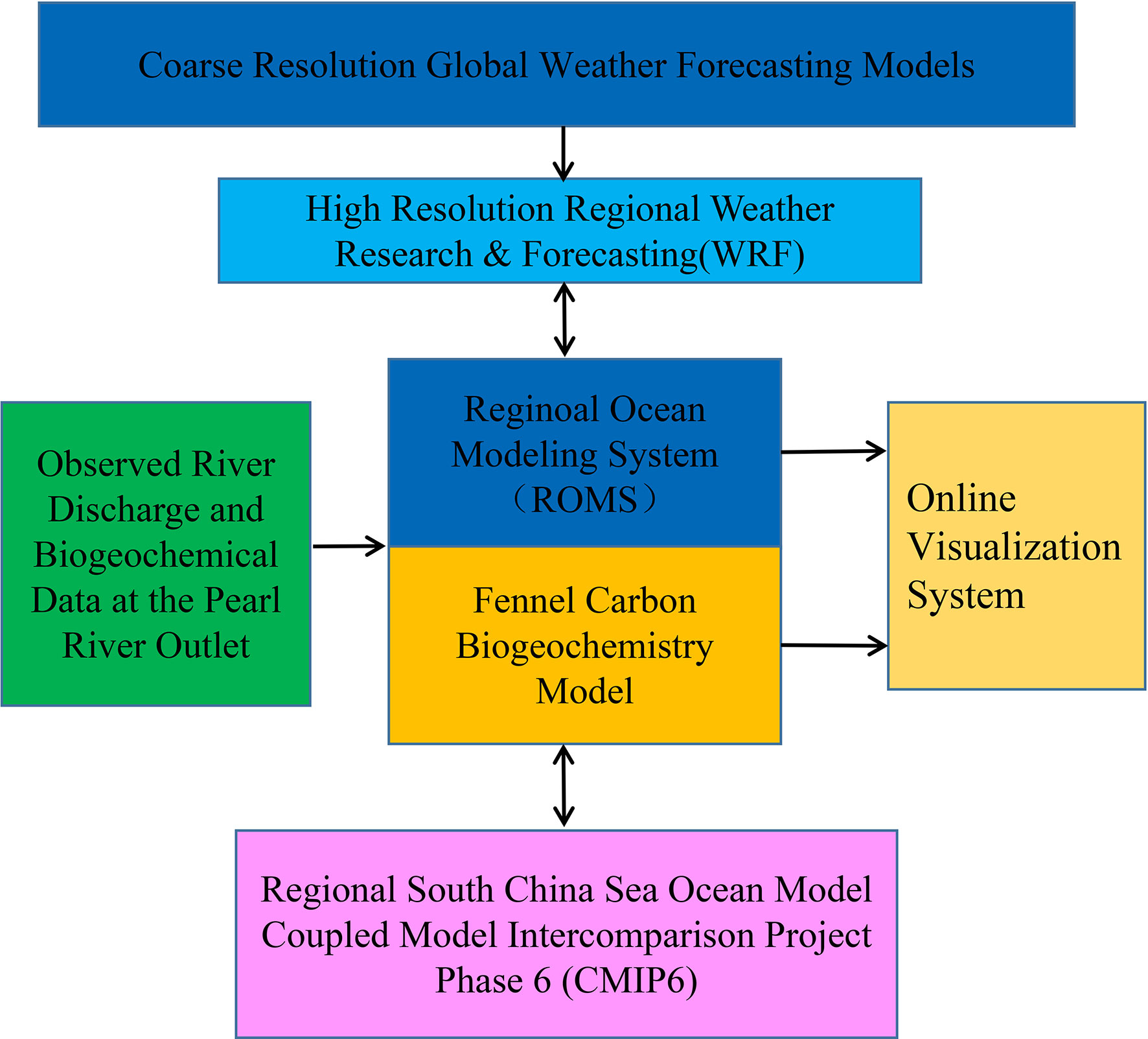
Figure 3 Flow chart of the forecast system automated workflow.

2.3 Observational data

We used a series of cruise observations from 2014 to 2018 to validate the model (Figure 4; Table 2). The observations are part of an ongoing program from a ship time-sharing project sponsored by the National Natural Science Foundation of China (NSCF) and Xiamen University. Measurements from Conductivity, Temperature, and Depth (CTD) sensors documented the vertical structure and monthly temperature, salinity, and DO. Chlorophyll, NO₃, NH₄, and pH levels were measured in the laboratory.

FIGURE 4

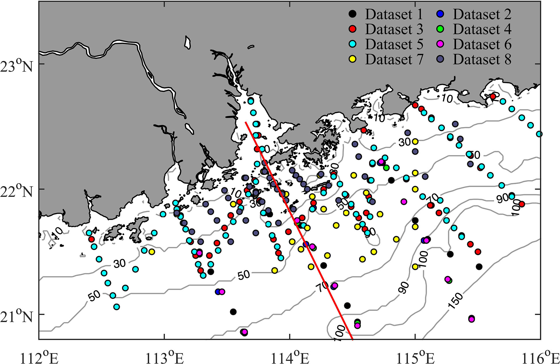
Figure 4 Sampling stations on the North South China Sea (NSCS) shelf off the PRE from multiple open cruises. The survey time is listed in Table 1. The red line shows the location of the vertical section in Figures 7, 5, and 11.

TABLE 2

Table 2 The survey time and variables of datasets 1–8 from the cruises.

2.4 Model skill metrics

Quantitative model–data comparisons using multiple skill metrics are critical because they highlight the advantages and potential limitations of a particular model, which must be carefully considered before using the model as a tool for scientific study or decision-making (Jolliff et al., 2009; Stow et al., 2009). In this analysis, multiple skill metrics were examined. This included the correlation coefficient the that measures the tendency of the model and observed values to covary, and was calculated as

$\begin{array}{ll}\text{r}=\frac{{\sum }_{i=1}^n(O_i-\overline{O})(M_i-\overline{M})}{\sqrt{{\sum }_{i=1}^n{(O_i-\overline{O})}^2{\sum }_{i=1}^n{(M_i-\overline{M})}^2}}& (18)\end{array}$

where O_i is the observation at time t_i, M_i is the model estimate at t_i, $\overline{O}$ is the mean of the observations, $\overline{M}$ is the mean of the model estimates, and n is the total number of observations available for comparison with model estimates. The bias, unbiased root–mean–squared difference (unbiased RMSD), and total root–mean–squared difference (RMSD) were calculated as:

$\begin{array}{ll}\text{Bias}=\frac{{\sum }_{i=1}^n(M_i-O_i)}{n}= \overline{M}-\overline{O}& (19)\end{array}$

$\begin{array}{ll}\text{unbiased RMSD}=\sqrt{\frac{{\sum }_{i=1}^n{[(M_i-\overline{M})-(O_i-\overline{O})]}^2}{n}}& (20)\end{array}$

$\begin{array}{ll}\text{RMSD}=\sqrt{\frac{{\sum }_{i=1}^n{(M_i-O_i)}^2}{n}}& (21)\end{array}$

These three skill assessment statistics are particularly useful as bias reports of the size of the model-observation discrepancies. Bias values near zero indicate a close match. However, this can be misleading because negative and positive discrepancies can cancel each other. The unbiased RMSD nullifies the effect of the mean and is a pure measure of how model variability differs from observational variability. Total RMSD provides an overall skill metric, given that it includes components for assessing mean (bias) and variability (unbiased RMSD).

2.5 Target and Taylor diagrams for model validation

Multiple model skill metrics are compactly visualized on Taylor (Taylor, 2001) and target diagrams (Hofmann et al., 2008; Friedrichs et al., 2009; Jolliff et al., 2009). For the Taylor diagram, in addition to these skill metrics, the model standard deviation, σ_m has also been calculated.

$\begin{array}{ll}{\sigma }_m=\sqrt{\frac{{\sum }_{i=1}^n{(M_i-\overline{M})}^2}{n}}& (22)\end{array}$

For both types of diagrams, skill statistics are typically normalized by the observational standard deviation (σ_o). This allows plotting of multiple different datasets on the same diagram.

$\begin{array}{ll}{\sigma }_O=\sqrt{\frac{{\sum }_{i=1}^n{(O_i-\overline{O})}^2}{n}}& (23)\end{array}$

The Taylor diagram is plotted using a polar coordinate system and summarizes the skill metrics, including r, σ, and unbiased RMSD. In contrast, the target diagram was plotted using a Cartesian coordinate system and summarized the total RMSD, unbiased RMSD, and bias. On the normalized Taylor diagram, the reference point at (1, 0) represents a perfect skill score. Meanwhile, on the target diagram, the center of the target (0, 0) represents a perfect skill score.

3 Results

3.1 Hindcast simulations for evaluating model accuracy

The hindcast simulation of sea surface salinity was in strong agreement with the observations for all eight cruises (Figure 5). The correlation coefficient was 0.89. The bias and RMSD were 0.83 and 2.77 PSU, respectively. The simulated sea surface salinity showed that the river plume exhibited multiple shapes during the eight cruises. It spread easterly in July, August, and September 2015 (Figures 5A, B, H) and along the west coast in October 2017 (Figure 5D). The river plume bulged offshore in June and August 2018 (Figures 5E, F), and symmetrical alongshore in September 2016 and June 2017 (Figures 5B, C). The simulated plume morphology is consistent with previous observational facts reported in literature that the Pearl River buoyant plumes formed during summer can be classified into four types, namely offshore bulge spreading, west alongshore spreading, east offshore spreading, and symmetrical alongshore spreading. These were predominantly determined by the combined effect of river discharge and wind (Chen et al., 2017; Luo et al., 2012; Zu and Gan, 2015; Ou et al., 2009). River discharge has regulated the plume size, while wind has played an important role in changing the plume shape. The east and southeast winds drive the buoyant plume westward, resulting in the plume spreading westward alongshore. Given that the river plume resides at the surface, it is susceptible to the surface Ekman effect. The southwest wind upwelled and detached the eastward plume off the coast, which then spread offshore. If the wind is purely in a southerly direction, the plume is confined nearshore and moves both eastward and westward, thus forming a symmetrical structure.

FIGURE 5

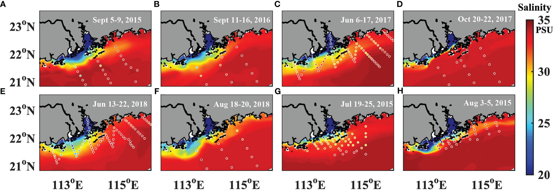
Figure 5 Comparison between observed (dots) and simulated (background color) surface salinity (< 2 m) for datasets (1) to (8) (Corresponding to A–H). The model results were assessed in the same time period as the observation.

Next, we compared the CGEEPS hindcast temperature and salinity along the vertical transect for six cruises where profiled CTD data were available (Figure 6). The simulated temperature and salinity were in strong agreement with the observations. For temperature, the CGEEPS hindcast replicated the observational fact that there was a strong thermocline in September 2015 and 2016, June 2017 and 2018, and August 2019, but not in October 2017. The correlation coefficient was 0.81. The bias and RMSD was 0.36 and 1.74 °C, respectively. The formation of a strong thermocline was due to upwelling of cold water under southwesterly winds, which generally occurs from June to August.

FIGURE 6

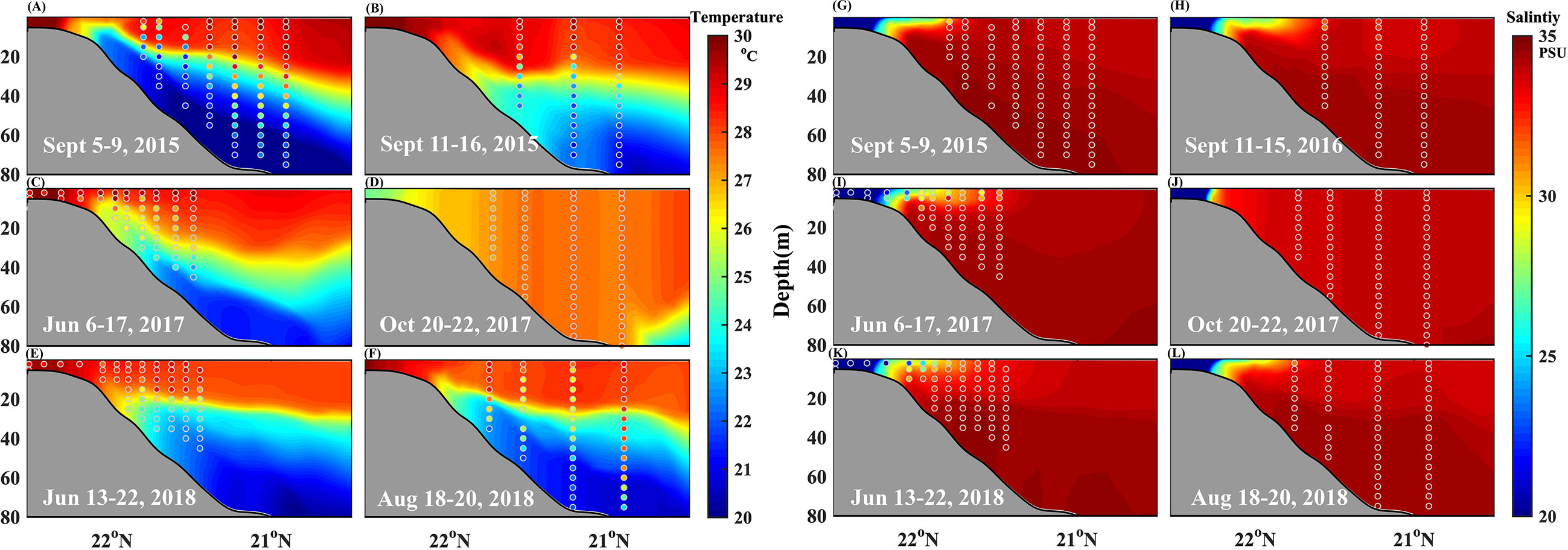
Figure 6 Comparison between observed (dots) and simulated (background color) temperature (A–F) and salinity (G–L) along vertical section for datasets (1) to (6).

In addition to the thermocline from upwelling, the low salinity riverine water extended further offshore with the southwesterly wind in both the CGEEPS hindcast simulation and observations. The 28 psu isohaline extended over 22 °N. However, October 2018 was highly favorable for the occurrence of downwelling conditions. The low salinity water was increasingly confined adjacent to the river mouth and the isohalines were vertically distributed. The correlation coefficient was 0.94 and the bias and RMSD were 0.19 and 1.78 psu, respectively.

The high level of skill in terms of temperature and salinity fields suggested that our modelling system was relatively robust in replicating the dynamics of the PRE–ocean system, which is a river-dominated margin (Rabouille et al., 2008).

We subsequently examined how the nitrogen type nutrients, which are a combination of NO₃ + NO₂ + NH₄, were reproduced by CGEEPS. Given that rivers and upwelling are the two main sources of nutrients, we initially observed that the concentrations of N-type nutrients can reach as high as 150 μM inside the estuary and decrease to less than 1 μM as the plume water extends offshore. The nitrate concentration was relatively high (5–10 μM) at 20 m from the bottom owing to upwelling (Figure 7). The correlation coefficient between simulated and observed NO₃ was 0.91; however, the bias seemed to be slightly larger (Bias = 20.79 μM, RMSD = 63.1 μM). We examined the output data and found that NO₃-overestimation predominantly occurred at three stations in the upper reaches of the estuary closer to the river mouth boundary of the model grid. This overestimation was likely because we had set up at the river mouth in the upper part of Lingding Bay rather than at the actual river mouth. If we excluded these three points from the calculation, the bias and RMSD were almost halved (Table 3).

FIGURE 7

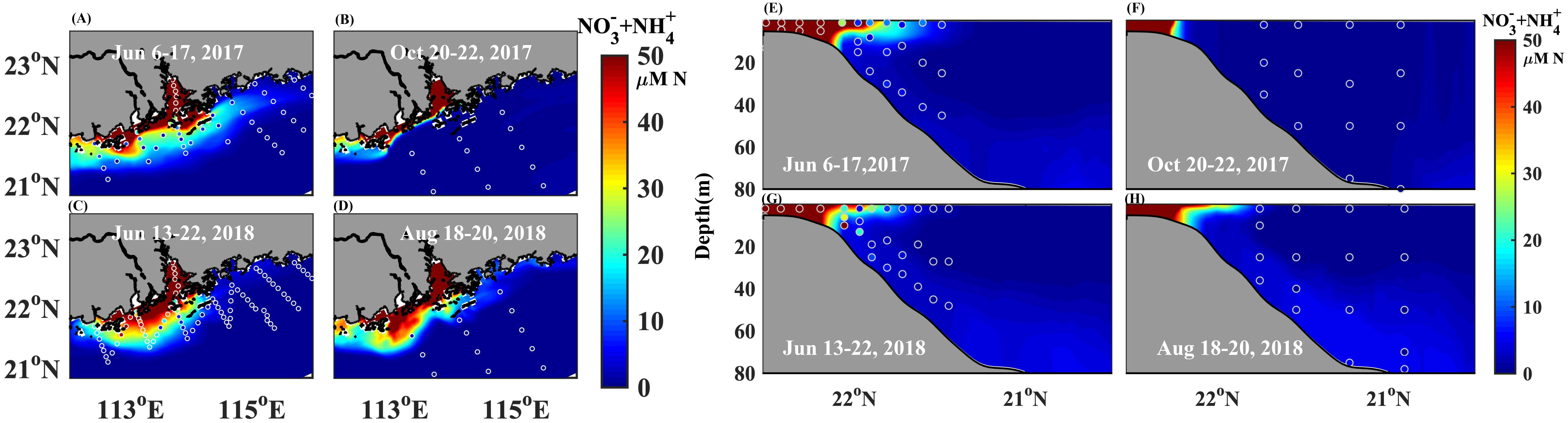
Figure 7 Comparison between observed and simulated nitrogen type nutrients (NO₃ + NO₂ + NH₄) for the surface (A–D) and along vertical transect (E–H) for datasets (3) to (6).

TABLE 3

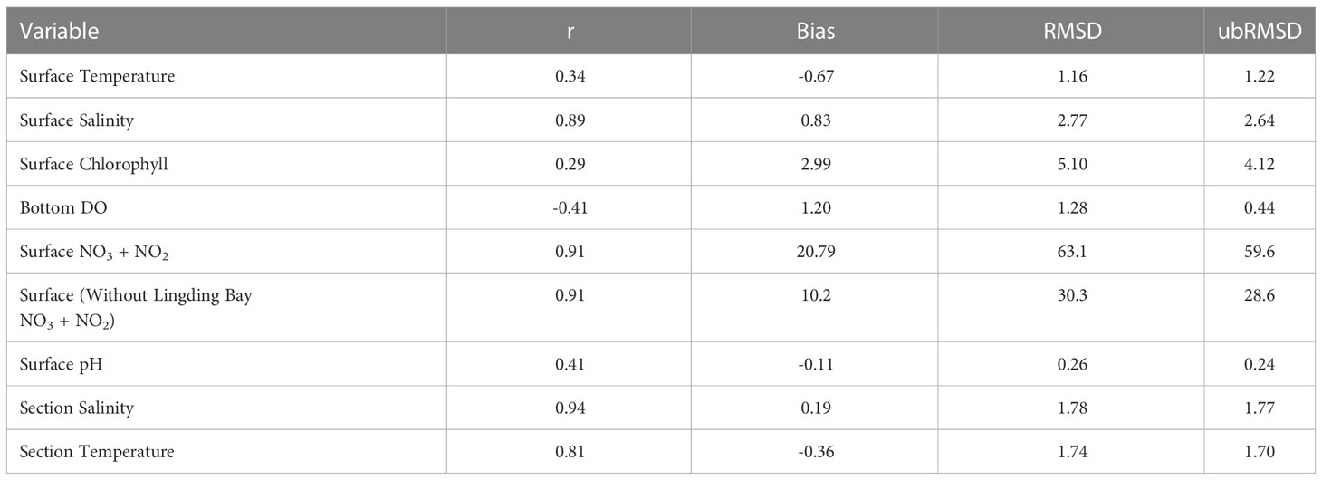
Table 3 Model evaluation statistics for 2015–2018.

The nutrient distribution was in line with the salinity distribution pattern in the river plume region, which were the two variables with the best performance in the simulation system.

The full model observation skill assessment is presented in Table 3. The comparison was conducted by gathering all the observational points and extracting the model output at the observational stations. This implies that the skill number incorporated both spatial and temporal variability. In addition to the temperature, salinity, and N-type nutrients, we also examined the model performance for surface chlorophyll concentration and bottom DO (Table 3). The comparison results showed that the correlation between the observed and simulated surface chlorophyll content was 0.29. The surface chlorophyll concentration was overestimated by approximately 3 μg–Chl/L, particularly in the plume area. This was likely due to the deficiency of the current ecosystem module in CGEEPS. To date, we have not incorporated the P- and light-limitation effects due to resuspended sediment. We expected that further incorporation of these processes would slow the growth of phytoplankton and decrease the surface chlorophyll concentration.

Although the surface chlorophyll concentration had been overestimated, the subsurface high chlorophyll maximum (DCM) structure was reproduced by the model (not shown here). The DCM layer lies immediately above the upwelled high NO₃ concentration, where nutrients and light were determined to be sufficient.

We further estimated the model’s overall ability to reproduce bottom DO and surface pH. The model’s skill in producing surface chlorophyll concentration and bottom DO was relatively poor. The correlation coefficient was positive at 0.41 for surface pH, but negative at −0.41 for bottom DO. The surface pH was underestimated by approximately −0.11 and the bottom DO was overestimated by approximately 1.2 mg/L. The underestimation of pH was likely associated with the surface temperature being underestimated by the model. This resulted in more dissolved CO₂ being held in the water and more hydrogen ions being released, resulting in lower pH values. The bottom DO was overestimated by the model, which was unexpected because the surface DO chlorophyll overestimated and more oxygen-consuming materials should be available. This overestimation may be because the current version of the biogeochemistry model did not include sediment oxygen consumption (SOC). Currently, the biogeochemistry model assumes that organic matter is immediately consumed upon reaching the bottom, whereas measurements show that organic matter consumption can be taken up over months. Instead of remaining in the same location, it is transported as fluid mud and undergoes numerous cycles of resuspension and deposition. The movement and long-term retention of organic matter in the sediment layer consumes additional oxygen when decomposed by bacteria. The current version of the carbon biogeochemistry model does not include the dissolved form of organic matter, which is another significant pool reserving organic matter and consuming DO. The current model parameter selections are predominantly empirical without optimization, which introduces considerable uncertainty to the simulated biogeochemical variables.

Table 3 provides the overall skill of the model by compiling multiple cruise data. However, it was not known how the model reflects spatial and temporal variability. Next, we performed a cruise-by-cruise comparison, which provided more specific information on the model’s skill in replicating the spatial variability of multiple variables. Both Taylor and target diagrams were introduced to graphically and quantitatively visualize multiple model skill metrics (Figure 8). For the predicted environmental variables at the surface and on the bottom, the model performances for salinity and temperature were uniform for all cruises. For salinity, the bias and RMSD were lower than 2 and 3.6 PSU, respectively, but the correlation coefficients were higher than 0.9. However, for temperature, both the bias and RMSD were low, and the correlation coefficients were also low (Figures 8A, B). In contrast to salinity and temperature, the performance of biogeochemical variables, especially surface chlorophyll, was cruise dependent. The model output showed a small bias and RMSD in October 2017, but a large bias and RMSD in June 2017. Similarly, the correlation coefficient was −0.08 in October 2017 but reached 0.61 in August 2018. Although the overall correlation coefficients for surface pH and chlorophyll concentration were 0.41 and 0.29, respectively, the correlation coefficient for a single cruise can reach as high as 0.7. These results suggest that surface chlorophyll and pH are more challenging to predict than temperature and salinity, because ecological and biogeochemical processes generally have larger uncertainties than physical processes.

FIGURE 8

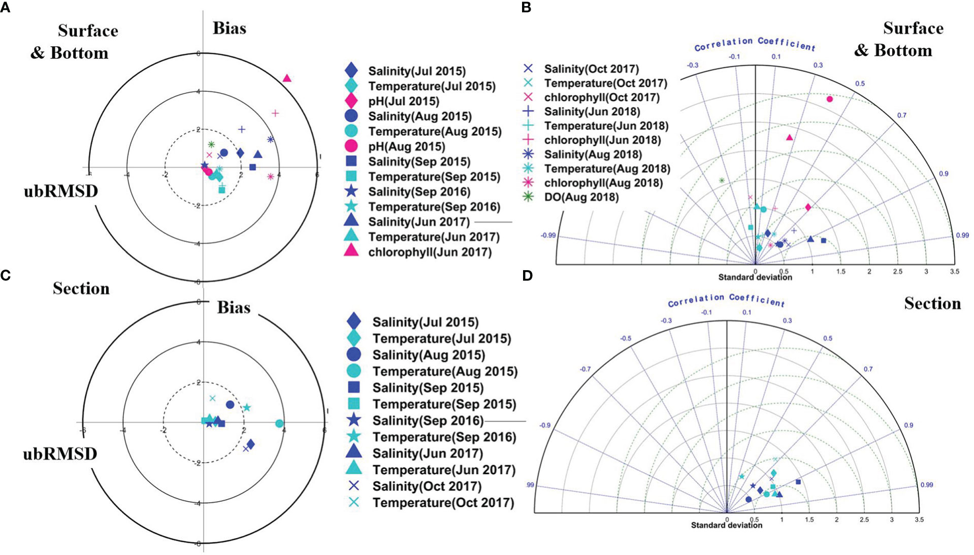
Figure 8 Target and Taylor diagrams displaying model skills for multiple hindicast variables between 2015 to 2017 individually on surface and bottom (A, B) and Sections (C, D). Each marker shape represents a different cruise.

Sectional data are only available for salinity and temperature. They showed a small bias and RMSD for all cruises. The correlation coefficients are over 0.7 for most cruises, except in September 2016, when the correlation coefficient for temperature was approximately 0.4.

Currently, data from multiple cruises are not collected at the same locations. Therefore, the ability of the model to reproduce temporal variability has not yet been assessed. Raw cruise data are processed using multiple laboratories. This implied that we could not guarantee that the same criteria and standards would be followed during data collection and preliminary processing. Therefore, the data quality itself may degrade the overall performance. We expect a future observational network and data-sharing platform to be set up in this region, which would benefit the systematic evaluation of the simulation performance in the future.

3.2 Differences in physical and biogeochemical fields by coupling with regional atmospheric model

Most coupled ocean–biogeochemistry model use atmospheric reanalysis products as forcing. One advantage of CGEEPS is the coupling of the regional atmospheric model with the regional ocean model. Compared to reanalysis products, the regional model usually has a high spatio-temporal resolution and the feedback of SST to the atmosphere. The coupled model has unique advantages in terms of simulating hurricane tracks and intensity. Therefore, we examined how the coupling technique has impacted ocean dynamics and biogeochemistry by using Hurricane Hato (2017) as an example.

Hurricane Hato formed over the western North Pacific at 128 °E, 20.4 °N on August 21, 2017. It moved westward and passed the Luzon Strait at approximately 0000 UTC on August 22 and intensified into a Category 1 typhoon by 0800 UTC on August 22, with maximum sustained near-surface wind speeds increasing to 33 ms⁻¹. At 0000 UTC on August 23, Hato was upgraded to a Category 2 typhoon with a maximum sustained near-surface wind speed of 42 ms⁻¹. Approximately 3 h later, Hato reached its peak intensity with a maximum sustained near-surface wind speed of 48 ms⁻¹. Hato made landfall near Zhuhai City (113.2 °E, 22.1 °N), Guangdong Province, at 0450 UTC on August 23. Soon after its landfall, Hato weakened rapidly to 30 ms⁻¹ over several hours and dissipated by 0800 UTC on August 24.

Two simulations were conducted from August 07 to September 05, 2017, the month when Hurricane Hato (2017) passed through. One was undertaken using two-way coupling with high-resolution regional configured WRF and the other by one-way forcing with coarse-resolution global ERA5. The simulated tracks of typhoons across the NSCS during August 22–24, 2017 are shown in Figure 9. The differences in both physical and biogeochemical fields are shown in Figures 10, 11.

FIGURE 9

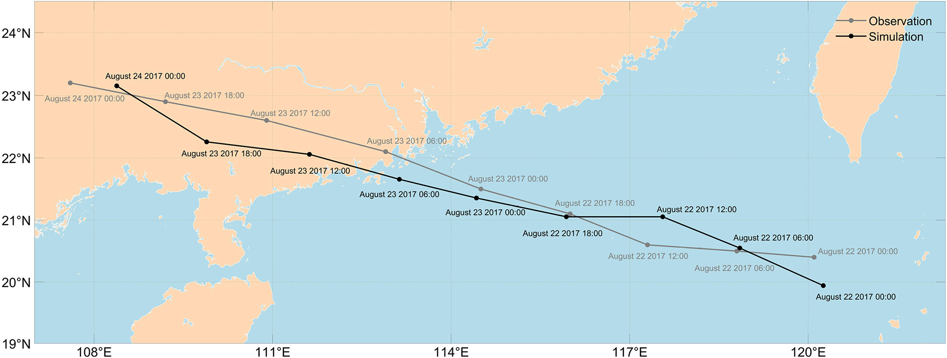
Figure 9 The observed and simulated track of Hurricane Hato (2017). The six-hour best-track TC data were obtained from the Shanghai Typhoon Institute.

FIGURE 10

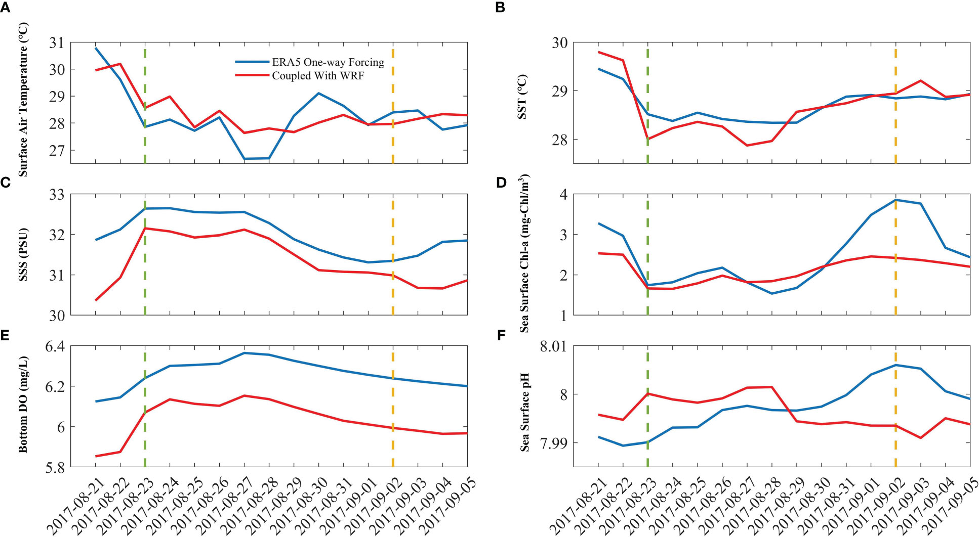
Figure 10 Surface air temperature (A), sea surface temperature (SST) (B), sea surface salinity (SSS) (C), sea surface chlorophyll (D), bottom DO (E), and sea surface pH (F) when forcing by one-way ERA5 atmosphere (blue lines) and two-way weather research forecasting (WRF; red lines). Vertical dashed lines depict timings for Hato (2017) passing by the PRE. The simulated passage of Hurricane Hato (2017) is shown in Figure 9.

FIGURE 11

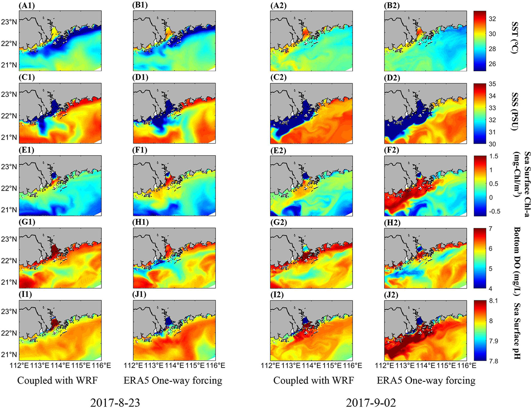
Figure 11 Comparison of horizontal distribution of SST, SSS, sea surface chlorophyll, bottom DO, and surface pH between ERA5 one-way atmospheric forcing (A, C, E, G, and I) and WRF two-way forcing (B, D, F, H, and J). Snapshots were selected during (August 23, 2017) and 11 d (September 02, 2017) after the typhoon.

We initially found that the typhoon tracks under the two runs were comparable. This indicates that the track of the typhoon was predominantly controlled by the background of large-scale atmospheric circulation (Figure 9).

For both runs, SST decreased and SSS increased rapidly from August 22 to August 23, 2017 (Figures 10B, C). This was caused by strong vertical mixing induced by the high wind of the hurricane. The SST increased after August 23 and decreased again from August 26. This was caused by upwelling after the eye passed offshore. The magnitude of the temperature drop from August 26 to August 28, 2017, in the two-way coupling WRF run was smaller than that in the one-way ERA5 run. This was likely because SST feedback to the atmosphere during the coupling weakened the strength of the tropical cyclone. The SST recovered from 28 August in both runs. However, the coupled WRF run diverged from the ERA5 one-way run from 31 August by maintaining a high SST at approximately 29°C. At the same time, the tropical cyclone brought heavy precipitation. This resulted in lower SSS in the two-way coupled WRF run than in the ERA5 one-way run.

Due to SST feedback to the atmosphere, we found that the difference between the two runs for surface air temperature (0.57 °C) was larger than SST (0.34 °C) (Figure 10A). The sea surface salinity was maintained at approximately 32 °C until August 27, 2017, and subsequently decreased. This was because river runoff increased after hurricane-induced heavy rainfall, which introduced a substantial amount of freshwater to the region being studied. The simulated results are consistent with the previous studies on ocean SST cooling and enhanced vertical mixing during a passage of a typhoon (Shen et al., 2021).

Surface chlorophyll, bottom DO, and surface pH varied with SSS and SST (Figures 10D–F). The temporal variability of chlorophyll, DO, and pH are strongly related to each other, that is, higher chlorophyll concentrations result in lower DO and higher pH. High surface chlorophyll concentrations indicate high primary production, which indicates that more oxygen-consuming materials are generated and DO decreases. A higher primary production also results in a higher pH because the equilibrium of carbonate ionization moves left after CO₂ is taken up by photosynthesis, thereby decreasing the concentration of hydrogen ions and increasing the pH value.

Owing to the strong vertical mixing induced by the hurricane, the surface chlorophyll concentration decreased, bottom DO increased, and surface pH decreased (Figures 10D–F). During the upwelling period when SST decreased, surface chlorophyll increased, bottom DO decreased, and surface pH also increased, which was caused by high primary production stimulated by sub-surface high nutrients. When the SSS decreased, the surface chlorophyll increased, the bottom DO decreased, and the increase in surface pH became larger.

A comparison between the two-time series and the two runs showed that the surface chlorophyll concentrations yielded larger differences than the SST and SSS differences. During Hato’s (2017) passage, although the chlorophyll concentration decreased in both runs, the average surface chlorophyll concentration in the ERA5 run was approximately 2.5 μg–Chl/L higher. The concentration differences were approximately 6.0 μg–Chl/L two weeks later (September 02, 2017). This suggests that the physical and biological processes are highly nonlinear. A minor change in the physical field may be enlarged several times in biogeochemical fields.

For a better view of the differences, we plotted the horizontal distribution of these variables for August 23 and September 02, 2017. During hurricane Hato’s (2017) passage and 11 d after it had passed, was when increased runoff substantially impacted biogeochemical processes.

On August 23, 2017, typhoons Hato induced strong vertical mixing and onshore currents, resulting in low-temperature water mixing up to the surface and confinement to the narrow nearshore band (Figure 11). Low salinity and riverine waters were predominantly confined to Lingding Bay. As a result, there was relatively higher chlorophyll and lower DO within Lingding Bay and adjacent to the nearshore western bank. As river discharge increased and was delivered to the coastal ocean, the plume water extended offshore. As a result, high surface chlorophyll, low DO, and high pH water also extended further offshore. The low salinity, high chlorophyll, and bottom DO water in the one-way ERA5 run occupied a larger area than that in the coupling WRF run. This was likely because the regionally configured WRF had a higher resolution than the one-way ERA5, which induced high sub-grid vertical mixing.

3.3 Forecasts for eutrophication, hypoxia, and ocean acidification

Although our simulation system may not have an exact accuracy in replicating the absolute value of all environmental variables at present, it is relatively informative in predicting variability under extreme weather conditions, such as floods and droughts.

The Pearl River Basin experienced a rainstorm in June 2022, which rapidly increased river discharge to 6×10⁴ m³s⁻¹ on June 15 (Figure 12A). CGEEPS successfully captured the surface salinity decrease associated with a sudden increase in runoff (Figure 12B). Compared to June 01, 2022, a low-salinity bulge formed on June 15 beside Lingding Bay (Figure 13B). The sudden increase in runoff also delivered more nutrients from land to the estuarine shelf, leading to phytoplankton blooms and a decrease in bottom dissolved oxygen (Figures 12E, F). At the surface, the low-salinity bulge was accompanied by a high NO₃ concentration (Figure 13D). However, the surface chlorophyll water was not synchronized with surface salinity and NO₃, which was relatively low within Lingding Bay and nearshore, but relatively high offshore (Figure 13H).The surface chlorophyll concentration depends on the relative importance of flushing and phytoplankton growth. High runoff reduces the residence time of phytoplankton, flushing them nearshore. Although the nutrient concentration was relatively high, there was insufficient time for phytoplankton to take up nutrients. Therefore, surface chlorophyll concentration was maintained at a low level. In contrast, phytoplankton had sufficient time to uptake NO₃ and bloom in the offshore region. We observed that high surface chlorophyll water was accompanied by higher pH levels. The pH was regulated by primary production. River runoff also brought a mass of DIC, resulting in a significant decrease in pH adjacent to the river mouth (Figure 13H). We also observed a sudden decrease in pH on June 16 from the time series after the peak discharge (Figure 12D).

FIGURE 12

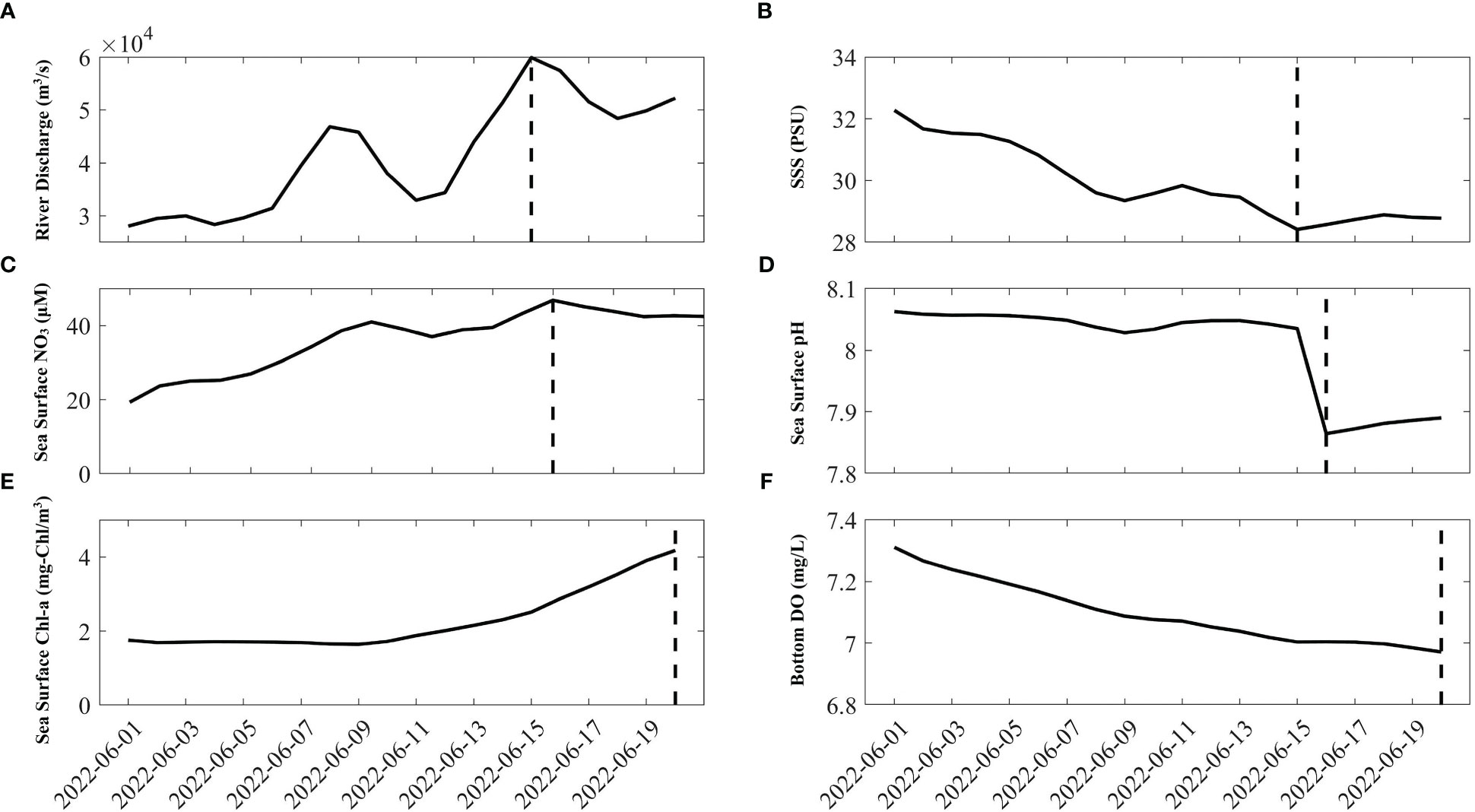
Figure 12 The river discharge (A) and CGEEPS predicted SSS (B), Sea surface NO₃ (C), pH (D), Chlorophyll (E), and bottom DO (F) from June 01, 2022, to June 20, 2022, when the flood happened. Vertical lines denote timing of maximum river runoff, sea surface NO₃, chlorophyll, and minimum sea surface salinity, surface pH and bottom DO.

FIGURE 13

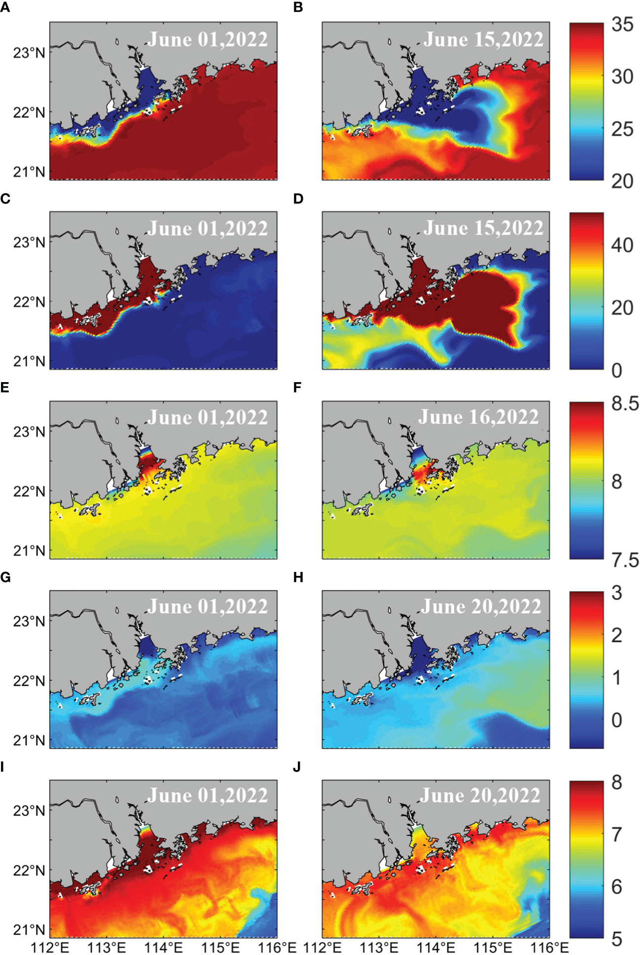
Figure 13 Comparison of SSS (A, B), Sea Surface NO₃ (C, D), pH (E, F), Chlorophyll (G, H), and bottom DO (I, J) before (June 01, 2022) and after flood occurrence (June 15, 2022). The snapshot dates are June 15, 2022 for surface salinity and NO₃; June 16, 2022 for surface pH; and June 20, 2022 for surface Chlorophyll and bottom DO.

These results suggest that the PRE and adjacent seas became more eutrophic, hypoxic, and acidic due to flooding. CGEEPS can capture such temporal and spatially varying environmental conditions, which can facilitate stakeholders making daily decisions regarding their usage of the bay’s resources.

To make it easier for the governments and private users to access and understand relevant information, the information provided by the CGEEPS system should be presented in an easily accessible format. In addition to the near-real-time simulation system, CGEEPS also includes a real-time online data visualization system in which the visualized graph is published in a webpage format. Graphics generated from CGEEPS can nowcast environmental variables daily and forecast them over two days (Figures 14, 15). The focus has been on the horizontal distribution of variables in the first generation of the forecast system (http://zhujiangtest.xyz:8000/). To better inform governance and stakeholders, we have recently extended it to produce a vertical profiles and maps to display the subsurface structure, which is informative for visualizing eutrophic, hypoxic, and acidic water.

FIGURE 14

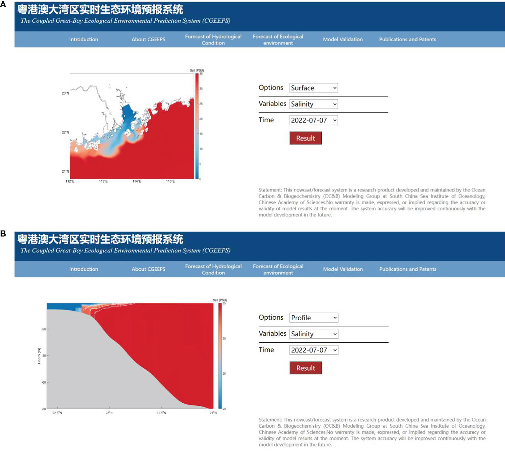
Figure 14 Real-time graphics displaying the surface (A) and vertical transect (B) of salinity (Screen shot from July 07, 2022).

FIGURE 15

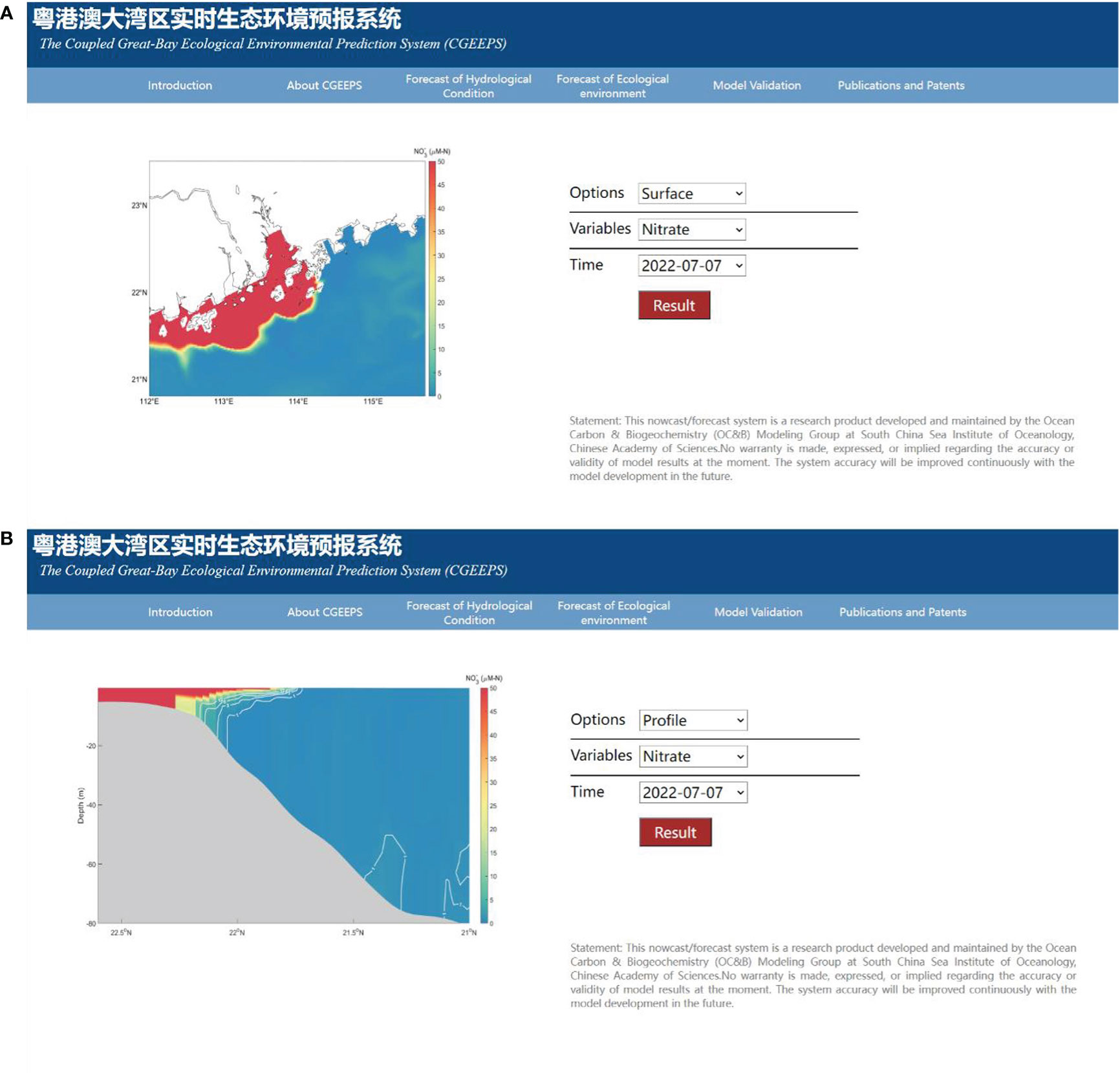
Figure 15 Real-time graphics displaying the surface (A) and vertical transect (B) of nitrate (Screen shot from July 07, 2022).

4 Discussion

Daily nowcasts and two-day forecasts from the ecological prediction system, the CGEEPS, were set up in the PRE and adjacent seas. The forecast systems were built on the COAWST modelling system. This comprises an atmospheric WRF module, an oceanic ROMS module, and a carbon-based biogeochemistry module (FENNEL). The forecast system can now provide real-time nowcast and two-day forecasts for temperature, salinity, NH₄ + NO₂ + NO₃, chlorophyll, DO, and pH. Hindcast comparison with available historical data from summer 2015–2018 has shown that the prediction system can replicate the temperature, salinity, and N-type nutrients for surface and vertical transects. However, the model performance for chlorophyll, DO, and pH was relatively poor. We also compared how the predicted biogeochemical fields differed from those predicted using coarse-resolution atmospheric reanalysis products. Using Hurricane Hato (2017) as an example, we found that stronger sub-grid vertical mixing was introduced after coupling with WRF. As a result, the surface salinity was lower than that when using coarse-resolution one-way ERA5 forcing. Due to the non-linear interaction between the physical and biogeochemical fields, the differences in surface chlorophyll became much greater than the salinity. Results suggest that the ecological environment prediction system was highly sensitive to physical forcing. The improved physical model would be beneficial to the system accuracy. We also determined how the physical and biological variables were predicted during the June 2022 rainstorm event. Results have shown that CGEEPS successfully captured data showing that the PRE and adjacent seas became fresher, more eutrophic, hypoxic, and acidic due to the Pearl River floods associated with the rainstorm. Results suggest that CGEEPS is capable of capturing the spatio-temporal variability of ecological environmental changes associated with extreme weather events.

At present, our ecological prediction system lacks accuracy in predicting some biological and biogeochemical environmental variables. We expect future improvements to increase system predictability, including: 1) more precise description of the water column and sediment processes, and 2) optimizing the parameter scheme of biogeochemical models. In addition to the modelling system itself, we found that building an observational network and data-sharing platform for this region was important. Compared to the Texas–Louisiana shelf, which is heavily impacted by the Mississippi River and Chesapeake Bay in the US, current observational data used to validate the system are relatively sparse and not spatially uniform. This increases the difficulty in evaluating the performance of the prediction system after new processes are introduced. An observational network has served as the basis for better parameterization of the ecosystem model. Another disadvantage of CGEEPS is that the system is currently operated and maintained manually, and we expect to use the Cron software utility to completely automate the CGEEPS workflow in the next phase of development.

Despite these disadvantages, CGEEPS is the first ecological environmental prediction system for the China Great Bay Area. The Hong Kong University of Science and Technology model data platform (http://ocean.ust.hk:8080/SiteMapApi/new/index.jsp) provides data visualization for daily averaged ocean circulation, ecosystem, and hypoxia, but no forecasts for these fields. Another example is the real-time Regional Forecast System of the SCS Marine Environment (https://epanf.scsio.ac.cn/), which is used to predict ocean circulation, waves, and several other important ocean–atmospheric dynamic variables rather than ecological environmental conditions (Zhu et al., 2020). Real-time environmental forecasting systems based on coupled ocean–atmosphere have also been set up worldwide. The Coupled Northwest Atlantic Prediction System (CNAPS), which is run by the North Carolina State University, predicts marine weather, ocean waves, and ocean circulation daily over an extensive area of the coastal northwest Atlantic Ocean. Another example is the South Eastern Levantine Israeli Prediction System (SLEIPS), which was setup through the Princeton Ocean Model (POM) and Variational Initial and Forcing Platform (VIFOP) for the coastal zone of the south eastern corner of the Levantine Basin (https://isramar.ocean.org.il/isramar2009/selips/), which provides temperature, salinity, and sea current prediction every 24 h. Compared with these prediction systems, CGEEPS is capable of predicting ecological environmental variables based on the coupled ocean–atmosphere–biogeochemistry technique. However, many challenges on prediction accuracy were present because biogeochemical models are highly unconstrained and observation streams are much sparser than physical streams (Fennel et al., 2019).

Therefore, we implemented a coupled ocean–atmosphere technique for ecosystem and biogeochemistry prediction. However, for river-dominated ocean margins, such as the Pearl River estuarine–coastal system, the land delivers substantial amounts of nutrients, organic matter, and suspended sediments. These materials regulate the biogeochemical cycle of estuarine–coastal ocean systems; therefore, coupling with process-based land ecosystem models is required in the future. Such a land–estuary–ocean biogeochemistry model has been developed for the Chesapeake Bay system (Feng et al., 2015). However, only land delivered materials in one-year was cycling used, and river discharge was still the USGS measurements (Bever et al., 2021). Model coupling techniques, such as CPL7, are required to develop an operational system (Sun et al., 2020).

Coastal marine ecosystems are subject to multiple stressors, such as climate change and human land activities. Implementation of an ecological environmental prediction system is important for protective and adaptive measures in ocean ecosystems. The prediction tool that we have constructed is based on realistic representations of ocean circulation coupled with biogeochemical and ecological models, which can forecast short-term (days to weeks) to seasonal (months) time intervals. In addition to this type of model, statistics based artificial intelligence models have emerged and have been applied to coastal ocean biogeochemistry studies in recent years (Chen et al., 2019; Li X et al., 2020; Ou et al., 2022; Yu et al., 2022). Compared with the coupled hydrodynamic–biogeochemistry model, artificial intelligent models are more efficient and require less computational resources. However, the application of such models to ocean biogeochemistry is still in its early stages. Therefore, the predictability and results explainable for such a model require further investigation.

5 Concluding remarks

Warming, acidification, deoxygenation, and eutrophication of estuarine–coastal oceans have manifested in recent decades due to climate change and human land activities. Ecological environmental prediction systems are important tools that help decision-makers and the public implement protective and adaptive measures for ocean ecosystems. Based on the coupled ocean–atmosphere–biogeochemistry model, we constructed a real-time ecological environmental forecast system for the Pearl River Estuary (PRE), namely the Coupled Great Bay Ecological Environment Prediction System (CGEEPS). Compared to previous ecological prediction systems built for this region, CGEEPS can not only provide real-time nowcasts and two-day forecasts for chlorophyll but also DO and pH. Although limited in its absolute accuracy, the system is still informative for eutrophication, deoxygenation, and acidification, especially under extreme weather events. We expect the expansion of biogeochemical and ecological observational systems built for this region to help develop and apply such prediction tools in the future. Ultimately, the predicted data products can benefit the economic, environmental, and public safety needs of stakeholders and governments.

Data availability statement

The datasets presented in this study can be found in online repositories. The names of the repository/repositories and accession number(s) can be found below:; http://www.gbaycarbontest.xyz:8008/.

Author contributions

LL, ZM: These authors contributed equally to this work and share first authorship. They are responsible for the writing of this paper. WM, JH, YLi, YLiu, YH, YZhu: These authors contributed equally to this work. They are responsible for the setup, calibration, operation and maintenance of the Coupled Great Bay Ecological Environmental Prediction System. YF: She share senior authorship. She is in charge of the whole project. All authors contributed to the article and approved the submitted version.

Funding

This research was supported by the State Key Laboratory of Tropical Oceanography Independent Research Fund (grant no. LTOZZ2103), the State Key Laboratory of Tropical Oceanography, South China Sea Institute of Oceanology, Chinese Academy of Sciences (grant no. LTO2215), the Major Projects of the National Natural Science Foundation of China (Grant Nos. 41890851, U21A6001), and the Strategic Priority Research Program of the Chinese Academy of Sciences (Grant No. XDA19060503).

Acknowledgments

The authors thank use of the HPCC at the South China Sea Institute of Oceanology, Chinese Academy of Sciences.

Conflict of interest

The authors declare that the research was conducted in the absence of any commercial or financial relationships that could be construed as a potential conflict of interest.

Publisher’s note

All claims expressed in this article are solely those of the authors and do not necessarily represent those of their affiliated organizations, or those of the publisher, the editors and the reviewers. Any product that may be evaluated in this article, or claim that may be made by its manufacturer, is not guaranteed or endorsed by the publisher.

Supplementary material

The Supplementary Material for this article can be found online at: https://www.frontiersin.org/articles/10.3389/fmars.2023.1096435/full#supplementary-material

Supplementary Table 1 | Definitions of biogeochemical parameters used in state variable equations.

References

[NOAA]National Oceanic and Atmospheric Administration (2020a) Chesapeake Bay operational forecast system (CBOFS) (Accessed May 1, 2020). Internet.

Google Scholar

[NOAA]National Oceanic and Atmospheric Administration (2020b) Sea Nettles probability of encounters (Accessed May 1, 2020). internet.

Google Scholar

Bever A. J., Friedrichs M. A. M., St-Laurent P. (2021). Real-time environmental forecasts of the Chesapeake bay: Model setup, improvements, and online visualization. Environ. Model. Software 140, 105036. doi: 10.1016/j.envsoft.2021.105036

CrossRef Full Text | Google Scholar

Cai M., Li K. (2011). Economic losses from marine pollution adjacent to pearl river estuary, China. Proc. Eng. 18, 43–52. doi: 10.1016/j.proeng.2011.11.008

CrossRef Full Text | Google Scholar

Chen Z., Gong W., Cai H., Chen Y., Zhang H. (2017). Dispersal of the pearl river plume over continental shelf in summer. Estuarine Coast. Shelf Sci. 194, 252–262. doi: 10.1016/j.ecss.2017.06.025

CrossRef Full Text | Google Scholar

Chen S., Hu C., Barnes B. B., Wanninkhof R., Cai W.-J., Barbero L., et al. (2019). A machine learning approach to estimate surface ocean PCO2 from satellite measurements. Remote Sens. Environ. 228, 203–226. doi: 10.1016/j.rse.2019.04.019

CrossRef Full Text | Google Scholar

Feng Y., Friedrichs M. A., Wilkin J., Tian H., Yang Q., Hofmann E. E., et al. (2015). Chesapeake Bay nitrogen fluxes derived from a land-estuarine ocean biogeochemical modeling system: Model description, evaluation, and nitrogen budgets. J. Geophysical Research: Biogeosciences 120 (8), 1666–1695. doi: 10.1002/2015JG002931

CrossRef Full Text | Google Scholar

Fennel K., Wilkin J., Levin J., Moisan J., O'Reilly J., Haidvogel. D. (2006). Nitrogen cycling in the middle Atlantic bight: Results from a three-dimensional model and implications for the north Atlantic nitrogen budget. Global. Biogeochem. Cycles 20, GB3007. doi: 10.1029/2005GB002456

CrossRef Full Text | Google Scholar

Fennel K., Wilkin J., Previdi M., Najjar R. (2008). Denitrification effects on air-sea CO2 flux in the coastal ocean: Simulations for the northwest north Atlantic. Geophys. Res. Lett. 35, L24608. doi: 10.1029/2008GL036147

CrossRef Full Text | Google Scholar

Fennel K., Hetland R., Feng Y., DiMarco. S. (2011). A coupled physical-biological model of the northern gulf of Mexico shelf: model description, validation and analysis of phytoplankton variability. Biogeosciences 8 (7), 1881–1899. doi: 10.5194/bg-8-1881-2011

CrossRef Full Text | Google Scholar

Fennel K., Gehlen M., Brasseur P., Brown C. W., Ciavatta S., Cossarini G., et al. (2019). Advancing marine biogeochemical and ecosystem reanalyses and forecasts as tools for monitoring and managing ecosystem health. Front. Mar. Sci. 6. doi: 10.3389/fmars.2019.00089

CrossRef Full Text | Google Scholar

Friedrichs M. A. M., Carr M. E., Barber R. T., Scardi M., Antoine D., Armstrong R. A., et al. (2009). Assessing the uncertainties of model estimates of primary productivity in the tropical pacific ocean. J. Mar. Syst. 76 (1-2), 113–133. doi: 10.1016/j.jmarsys.2008.05.010

CrossRef Full Text | Google Scholar

HKUST Hong Kong University of Science and Technology (2020) Ocean circulation, ecosystem and hypoxia around Hong Kong waters (OCEAN-HK) (Accessed August 6, 2020). Internet.

Google Scholar

Hofmann E., Druon J.-N., Fennel K., Friedrichs M., Haidvogel D., Lee C., et al. (2008). Eastern US Continental shelf carbon budget: Integrating models, data assimilation, and analysis. Oceanography 21 (1), 86–104. doi: 10.1111/j.1468-2958.1996.tb00396.x

CrossRef Full Text | Google Scholar

Jefferson T. A., Hung S. K. (2004). A review of the status of the indo-pacific humpback dolphin (Sousa chinensis) in Chinese waters. Aquat. Mammals 30 (1), 149–158. doi: 10.1578/AM.30.1.2004.149

CrossRef Full Text | Google Scholar

Jolliff J. K., Kindle J. C., Shulman I., Penta B., Friedrichs M. A. M., Helber R., et al. (2009). Summary diagrams for coupled hydrodynamic-ecosystem model skill assessment. J. Mar. Syst. 76 (1-2), 64–82. doi: 10.1016/j.jmarsys.2008.05.014

CrossRef Full Text | Google Scholar

Lewis E. R., Wallace D. W. R. (1998). Program developed for CO2 system calculations (Oak Ridge, Tennessee: Oak Ridge National Laboratory Press). doi: 10.15485/1464255

CrossRef Full Text | Google Scholar

Li X., Bellerby R. G. J., Ge J., Wallhead P., Liu J., Yang A. (2020). Retrieving monthly and interannual total-scale pH (pH T) on the East China Sea shelf using an artificial neural network: ANN-pH T-v1. Geoscientific Model. Dev. 13 (10), 5103–5117. doi: 10.5194/GMD-13-5103-2020

CrossRef Full Text | Google Scholar

Li D., Gan J., Hui R., Liu Z., Yu L., Lu Z., et al. (2020). Vortex and biogeochemical dynamics for the hypoxia formation within the coastal transition zone off the pearl river estuary. J. Geophysical Research: Oceans 125 (8), e2020JC016178. doi: 10.1029/2020JC016178

CrossRef Full Text | Google Scholar

Liu J.-x., Song C. (2022). A historical investigation of oyster breeding industryin pearl river estuary during Ming and Qing dynasties. Chin. Fisheries Economics 40 (01), 115–122.

Google Scholar

LiveOcean: Pacific Northwest ocean and estuary forecasts (2020) Internet (Accessed May 1, 2020).

Google Scholar

Lu F.-H., Ni H.-G., Liu F., Zeng E. Y. (2009). Occurrence of nutrients in riverine runoff of the pearl river delta, south China. J. Hydrology 376 (1-2), 107–115. doi: 10.1016/j.jhydrol.2009.07.018

CrossRef Full Text | Google Scholar

Luo L., Zhou W., Wang D. (2012). Responses of the river plume to the external forcing in pearl river estuary. Aquat. Ecosystem Health Manage. 15 (1), 62–69. doi: 10.1080/14634988.2012.655549

CrossRef Full Text | Google Scholar

Ma Y., Wei W., Xia H., Yu B., Wang D., Ma Y., et al. (2009). History change and influence factor of nutrient in lingdinyang Sea area of zhujiang river estuary. Actaoceanologica Sin. 31 (2), 69–77. Chinese edition/Haiyang Xuebao.

Google Scholar

Mellor G. L., Yamada T. (1982). Development of a turbulence closure model for geophysical fluid problems. Rev. Geophys 20, 851–875. doi: 10.1029/RG020i004p00851

CrossRef Full Text | Google Scholar

Ou Y., Li B., Xue Z. G. (2022). Hydrodynamic and biochemical impacts on the development of hypoxia in the Louisiana–texas shelf – part 2: Statistical modeling and hypoxia prediction. Biogeosciences 19 (15), 3575–3593. doi: 10.5194/bg-19-3575-2022

CrossRef Full Text | Google Scholar

Ou S., Zhang H., Wang D.-x. (2009). Dynamics of the buoyant plume off the pearl river estuary in summer. Environ. Fluid Mechanics 9 (5), 471–492. doi: 10.1007/s10652-009-9146-3

CrossRef Full Text | Google Scholar

Peng S., Li Y., Gu X., Chen S., Wang D., Wang H., et al. (2015). A real-time regional forecasting system established for the south China Sea and its performance in the track forecasts of tropical cyclones during 2011–13. Weather Forecasting 30 (2), 471–485. doi: 10.1175/WAF-D-14-00070.1

CrossRef Full Text | Google Scholar

Qian W., Gan J., Liu J., He B., Lu Z., Guo X., et al. (2018). Current status of emerging hypoxia in a eutrophic estuary: The lower reach of the pearl river estuary, China. Estuarine Coast. Shelf Sci. 205, 58–67. doi: 10.1016/j.ecss.2018.03.004

CrossRef Full Text | Google Scholar

Rabouille C., Conley D. J., Dai M. H., Cai W.-J., Chen C. T. A., Lansard B., et al. (2008). Comparison of hypoxia among four river-dominated ocean margins: The changjiang (Yangtze), Mississippi, pearl, and rhône rivers. Continental Shelf Res. 28 (12), 1527–1537. doi: 10.1016/j.csr.2008.01.020

CrossRef Full Text | Google Scholar

Shchepetkin A. F., McWilliams J. C. (2009). Computational kernel algorithms for fine-scale, multiprocess, longtime oceanic simulations. Handb. Numerical Analysis. 14 (08), 121–183. doi: 10.1016/S1570-8659(08)01202-0

CrossRef Full Text | Google Scholar

Shen D., Li X., Wang J., Bao S., Pietrafesa L. J. (2021). Dynamical oceanresponses to typhoon malakas, (2016) in the vicinity of Taiwan. J. Geophysical Research: Oceans 126 (2), e2020JC016663. doi: 10.1029/2020JC016663

CrossRef Full Text | Google Scholar

Stedman S., Dahl T. E. (2008). Coastal wetlands of the eastern united states: 1998 to 2004, status and trends. Natl. Wetlands Newslett. 30 (4), 18–20.

Google Scholar

Stow C. A., Jolliff J., McGillicuddy D.J. Jr, Doney S. C., Allen J. I., Friedrichs M. A., et al. (2009). Skill assessment for coupled biological/physical models of marine systems. J. Mar. Syst. 76 (1-2), 4–15. doi: 10.1016/j.jmarsys.2008.03.011

PubMed Abstract | CrossRef Full Text | Google Scholar

Sun L., Liang X. Z., Xia M. (2020). Developing the coupled CWRF-FVCOM modeling system to understand and predict atmosphere-watershed interactions over the great lakes region. J. Adv. Modeling Earth Syst. 12 (12), e2020MS002319. doi: 10.1029/2020MS002319

CrossRef Full Text | Google Scholar

Taylor K. E. (2001). Summarizing multiple aspects of model performance in a single diagram. J. Geophysical Research: Atmospheres 106 (D7), 7183–7192. doi: 10.1029/2000JD900719

CrossRef Full Text | Google Scholar

Wang J. (1996). Global linear stability of the two-dimensional shallow-water equations: An application of the distributive theorem of roots for polynomials on the unit circle. Monthly Weather Rev. 124 (6), 1301–1310. doi: 10.1175/1520-0493(1996)124<1301:GLSOTT>2.0.CO;2

CrossRef Full Text | Google Scholar

Wang J. A. (2001). Nowcast/forecast system for coastal ocean circulation using simple nudging data assimilation. J. Atmospheric Oceanic Technol. 18 (6), 1037–1047. doi: 10.1175/1520-0426(2001)018<1037:ANFSFC>2.0.CO;2

CrossRef Full Text | Google Scholar

Wang W.-X., Rainbow P. S. (2020). Pollution in the pearl river estuary. Estuaries World. 23 (686), 23, 13–35. doi: 10.1007/978-3-662-61834-9_3

CrossRef Full Text | Google Scholar

Warner J. C., Armstrong B., He R., Zambon J. B. (2010). Development of a coupled ocean–atmosphere–wave–sediment transport (COAWST) modeling system. Ocean Model. 35 (3), 230–244. doi: 10.1016/j.ocemod.2010.07.010

CrossRef Full Text | Google Scholar

Warner J. C., Sherwood C. R., Signell R. P., Harris C. K., Arango H. G. (2008). Development of a three-dimensional, regional, coupled wave, current, and sediment-transport model. Comput. Geosciences 34 (10), 1284–1306. doi: 10.1016/j.cageo.2008.02.012

CrossRef Full Text | Google Scholar

Ye F., Guo W., Shi Z., Jia G., Wei G. (2017). Seasonal dynamics of particulate organic matter and its response to flooding in the pearl river estuary, China, revealed by stable isotope (δ13C and δ15N) analyses. J. Geophysical Research: Oceans 122 (8), 6835–6856. doi: 10.1002/2017JC012931

CrossRef Full Text | Google Scholar

Yu L., Gan J. (2021). Mitigation of eutrophication and hypoxia through oyster aquaculture: an ecosystem model evaluation off the pearl river estuary. Environ. Sci. Technol. 55 (8), 5506–5514. doi: 10.1021/acs.est.0c06616

PubMed Abstract | CrossRef Full Text | Google Scholar

Yu L., Gan J. (2022). Reversing impact of phytoplankton phosphorus limitation on coastal hypoxia due to interacting changes in surface production and shoreward bottom oxygen influx. Water. Res. 212, 118094. doi: 10.1016/j.watres.2022.118094

PubMed Abstract | CrossRef Full Text | Google Scholar

Zhou L., Wang G., Kuang T., Guo D., Li G. (2019). Fish assemblage in the pearl river estuary: Spatial-seasonal variation, environmental influence and trends over the past three decades. J. Appl. Ichthyology 35 (4), 884–895. doi: 10.1111/jai.13912

CrossRef Full Text | Google Scholar

Zhou L., Zeng L., Fu D., Xu P., Zeng S., Tang Q., et al. (2016). Fish density increases from the upper to lower parts of the pearl river delta, China, and is influenced by tide, chlorophyll-a, water transparency, and water depth. Aquat. Ecol. 50 (1), 59–74. doi: 10.1007/s10452-015-9549-9

CrossRef Full Text | Google Scholar

Zhu Y., Li Y., Peng S. (2020). The track and accompanying Sea wave forecasts of the supertyphoon mangkhut, (2018) by a real-time regional forecast system. J. Atmospheric Oceanic Technol. 37 (11), 2075–2084. doi: 10.1175/JTECH-D-19-0196.1

CrossRef Full Text | Google Scholar

Zu T., Gan J. (2015). A numerical study of coupled estuary–shelf circulation around the pearl river estuary during summer: Responses to variable winds, tides and river discharge. Deep Sea Res. Part II: Topical Stud. Oceanography 117, 53–64. doi: 10.1016/j.dsr2.2013.12.010

CrossRef Full Text | Google Scholar