 Jian Zheng
 Chuanshuo Mao
 Qiang Zhang
94% of researchers rate our articles as excellent or good
Learn more about the work of our research integrity team to safeguard the quality of each article we publish.
Find out more
ORIGINAL RESEARCH article
Front. Mar. Sci. , 21 March 2023
Sec. Marine Affairs and Policy
Volume 10 - 2023 | https://doi.org/10.3389/fmars.2023.1095283
This article is part of the Research Topic Global Vessel-Source Maritime Pollution Governance—Technical Innovation and Policy Orientation View all 14 articles
Uncertainties in port handling efficiency can cause port delays in the liner shipping system. Furthermore, policies on carbon emission reduction, such as EEXI standards, restrict the potential for speed optimization in liner shipping operations. Traditional tactical planning speed optimization is unsuitable for operational-level decision making, leading to unreliable schedules. From a schedule-reliability and energy-efficiency perspective, we propose a real-time speed optimization method based on discrete hybrid automaton (DHA) and decentered model predictive control (DMPC). We use a dynamic adjustment of sailing speed to offset the disturbance caused by port handling efficiency uncertainties. First, we establish a DHA model that describes each ship’s hybrid dynamics of state switching between sailing and berthing; then, we develop a prediction model for the DMPC controller, which is analogous to the DHA model. The schedule is transferred into time–position coordinates as controller reference trajectories in the receding horizon speed optimization framework. We consider determining tracking errors, carbon emissions, and fuel consumption as our objectives, and we carry out engine power limitation (EPL) analysis for the sample ship, which turns the EEXI standards into constraints. We attain the recommended speed by solving a mixed-integer optimization. We carry out a case study, and our results indicate the effectiveness of our proposed DHA-DMPC scheme in lowering port delays and achieving the best trade-off between schedule reliability and energy efficiency. Additionally, we conduct further experiments to analyze the impacts of various carbon reduction policies on the performance levels of liner shipping operations.
Ships operated by container shipping lines follow published schedules and travel along fixed routes with regular port rotations. However, the schedule reliability of liner shipping is often influenced by uncertain factors at ports. For instance, a labor strike would lead to decreases in the pace of port handling, while port congestion would lengthen the time ships are required to wait before berthing. These uncertain factors result in schedule unreliability and port delays, reducing the competitive advantages of liner shipping lines and disturbing the regularity of the global supply chain (Zheng et al., 2021). Ship speeding up is the most common approach to reduce port delays. Moreover, IMO has imposed new technical measures, such as the Energy Efficiency Existing Ship Index (EEXI), which will come into force on January 1, 2023, attempting to achieve long-term goals to reduce greenhouse gas emissions (ABS, 2021). Shipping companies may need to implement solutions such as engine power limitation (EPL) on their fleets to comply with the EEXI standard. However, EPL lowers the top limit of the adjustable ship speed, which has an impact on the controllability of reducing port delays through ship speeding up. Therefore, real-time speed optimization for liner shipping operations is required to eliminate port delays caused by unpredictable port handling efficiency, improve schedule reliability while complying with the EEXI standard, and maintain low operating costs.
Speed changes have a significant impact on fluctuations in fuel consumption and carbon emissions, which are proportional to the third power of sailing speed. As a result, determining the ideal sailing speed is crucial (Leaper, 2019; Dunn et al., 2021); therefore, speed optimization has become a hot topic in research on liner shipping operations (Jimenez et al., 2022). Speed optimization is used in tactical planning to determine the service speed between adjacent ports, and is carried out in combination with other tactical decisions, such as fleet deployment and schedule design (Notteboom, 2006; Brouer et al., 2017; Karsten et al., 2017; Chen et al., 2022). Traditional tactical-level planning often considers minimizing operating costs, fuel consumption, and carbon emissions as objectives, with the problem formulated as a mixed-integer programming (MIP) model (Fagerholt et al., 2010; Wang and Meng, 2012a). Some studies have expanded the model’s application scenarios, taking into account more tactical decisions, such as cargo allocation and bunker policy, transforming the model into an integrated decision support system. Psaraftis and Kontovas (2014) considered various factors affecting speed decisions, such as load, fuel price, market condition, etc. Wen et al. (2017) studied the speed optimization of heterogeneous fleets. In addition to voyage duration, cost, and emissions, the satisfaction of shippers is also an objective. Based on statistical data from a shipping line, Xia et al. (2015) fit the relationship between load, sailing speed, and fuel consumption. Both cargo allocation and speed optimization are included in the optimization model. Guericke and Tierney (2015) established an MIP model to maximize shipping lines’ profits and designed a decision support system that can recommend the optimal speed, freight rate, and cargo allocation plan. Sheng et al. (2015) combined ship refueling problems with speed determination. Pasha et al. (2021) proposed an integrated optimization model that addresses all the major tactical liner shipping decisions for heterogeneous fleets.
While the aforementioned studies are capable of figuring out tactical plans, they fail to take into account uncertain factors that might affect how effective the plan is. Some scholars attempted to quantify the level of the uncertainties using a probabilistic model, allowing the uncertain factors to be measured and balanced out by adding buffer time to the schedule (Wang and Meng, 2012b; Meng et al., 2014; An and Lo, 2016). Qi and Song (2012) used simulation-based stochastic approximation methods to consider uncertain port times and created a robust schedule aimed at maintaining a high service level. Aydin et al. (2017) developed a speed optimization model with stochastic port times and time windows and then determined the service speed using dynamic programming. Liu et al. (2020) studied speed optimization and bunker policy under uncertain demand conditions. Tan et al. (2018) proposed a joint ship schedule design and sailing speed optimization problem for a single inland shipping service considering uncertain dam transit time.
A robust tactical plan can be generated by quantifying uncertain factors in the optimization model. However, some uncertainties, such as labor strikes and weather conditions, are hard to predict and cannot be measured properly. It is impossible to consider these factors in the tactic-level optimization model. Furthermore, the service speed in tactical plans remains a fixed value for the voyage in adjacent ports and there are no indications for a ship to adjust sailing speed during a voyage. As a result, operational-level speed management incorporating real-time optimization is needed. In operational-level speed optimization studies, the voyage is typically broken into multiple legs, and the sailing speed on each leg is then computed using dynamic programming. (Perera and Mo, 2016; Lee et al., 2018; Wang et al., 2017; Li et al., 2018). Wang et al. (2018) proposed a nonlinear model predictive control framework based on real-time updated environmental information and applied a particle swarm optimization algorithm to compute the optimal speed. Therefore, the sailing speed can be adjusted to consider varying environmental factors and remain optimal throughout the whole voyage. Huotari et al. (2021) presented a novel convex optimization model for ship speed profile optimization under varying environmental conditions and timetable constraints. Tzortzis and Sakalis (2021) proposed a dynamic speed optimization problem, transforming the optimization problem into several sub-problems for improved weather forecasting by segmenting the full time horizon into smaller time regions.
Although the above optimization models can effectively balance uncertainties, they are only able to represent a single voyage with a single ship. A predominant characteristic of liner shipping operations is that the ships’ motions repeatedly switch between sailing and berthing. Such a characteristic complicates the modeling process for liner shipping operations; hence, a more detailed optimization model that describes this hybrid dynamic phenomenon is required. In this paper, we model a discrete hybrid automaton (DHA), and then a decentered model predictive control (DMPC) framework is designed. As we focus on operational-level speed management, we assume that the service speed, the fleet deployment, and the schedule have already been determined. Real-time speed optimization is realized through the receding horizon optimization method with the objectives of operating the ships on predetermined schedules while complying with the EEXI standard and maintaining high energy efficiency.
We present the contributions of our paper as follows:
(a) We formulate the hybrid dynamic phenomenon of liner shipping operations by a DHA model constructed using a mixed logical dynamical (MLD) approach, which precisely captures ships’ motions and state switching rules;
(b) For real-time speed optimization against uncertain port handling efficiency, we design a DMPC controller based on a receding horizon optimization strategy, in which the prediction model is built analogous to the DHA model and the schedule is transferred into a tractable reference trajectory. Ships’ sailing speeds can be adjusted to reduce possible port delays;
(c) Our optimization model incorporates the EEXI standard and converts it into a constraint to guarantee that the emission policy is met while maintaining schedule reliability.
The remainder of our paper is organized as follows: In Section 2, we construct the DHA model and design the DMPC framework. We present our case study and extend experiment results in Section 3. We discuss our findings in Section 4 before concluding our paper in Section 5.
There are two motions for ships in liner shipping operations: sailing state and berthing state. These two states switch between each other in circles, reflecting a hybrid dynamical phenomenon that involves both continuous states (sailing states and berthing states) and logic rules (judging when will the state switch happen). While sailing, a ship’s positions are updated in real time, and the ship switches into a berthing state when it reaches the corresponding ports. Container handling is done during berthing while the ship’s position remains unchanged. In this section, a DHA model is constructed to characterize the dynamics of the ships in liner shipping operations. The real-time dynamical states of each ship in the liner shipping fleet can be calculated. The DHA model serves two purposes: (a) The DHA model functions as a system plant to represent the reality of liner shipping operations and test the proposed sped optimization method. (b) A prediction model in the DMPC framework is established, analogous to the DHA model. As a key component of the DMPC system, the prediction model forecasts the future states of the ships based on their present states. The control effect is determined by the degree of forecast accuracy.
The DMPC controller is designed in Section 2.2. Real-time speed optimization is realized through the receding horizon optimization scheme. Moreover, the decentralized controller arrangement mode reduces individual controllers’ computing capacity and improves the system’s overall computing efficiency. The DMPC controller is supposed to timely adjust the ships’ sailing speed against uncertain port handling efficiency to reduce port delays and keep the liner shipping system in optimal performance.
We propose a DHA model based on a discrete-time framework constructed using the MLD modeling approach to formulate the hybrid dynamics of liner shipping operations (Sirmatel and Geroliminis, 2018). A discrete hybrid automaton (DHA) consists of four modules: a switched affine system (SAS), an event generator (EG), a mode selector (MS), and a finite state machine (FSM). The SAS module describes the continuous dynamics of the liner shipping operations and the FSM module represents the logical rules. The EG and MS modules realize the interconnections between continuous dynamics and logic rules. Continuous state variables in different ranges trigger corresponding discrete events through the EG module, while the MS module alters the continuous variables’ evolving modes following indications generated by the FSM module (Bemporad and Morari, 1999).
The SAS module describes how the continuous states of each ship evolve in different modes: sailing, berthing, and reset. Each ship is in a specific mode at any instant. In sailing mode, the ship’s position changes while the quantities of handled containers remain 0; however, the situation is reversed in the berthing mode. The ship enters reset mode when it accomplishes a round-circle voyage; then, its position is reset to 0 for a new voyage.
We consider a liner shipping system with a fleet of ships. The number of calling ports is and the total number of sailing legs is . The distance between adjacent ports in the rotation is called a leg.
(a) Position dynamics can be described as follows:
where is the sampling time; (n mile) represents the position of ship at instant ; and (knots) is the sailing speed of ship at instant . , , and represent three modes of sailing, berthing, and resetting, respectively.
(b) The dynamics of container handling can be expressed as follows:
where denotes the quantities of handled containers of ship at port , which is the total number of containers being loaded or unloaded, or any other terminal operations; furthermore, is set to 0 when the ship is sailing. expresses the container handling efficiency of port at instant . The port handling efficiency is defined as an average container handling rate at port, which is calculated through dividing the total quantities of handled containers by the total observable time at port.
Binary events are triggered when the EG module detects that the continuous state variables reach certain ranges. In the liner shipping system, the events are triggered by the values of ships’ positions and the quantities of their handled containers.
(a) Event triggered by position dynamics is as follows:
where describes whether ship has reached port or not. At instant , if ship has reached port , then is true; otherwise, is false.
(b) Event generated when ship i finishes a round-circle voyage is as follows:
where describes whether ship has finished a circle voyage or not.
(c) Event triggered by container handling dynamics is as follows:
where describes whether ship has finished container handling at port or not. is the container quantities to be handled for ship at port , which is acquired through observation. is triggered when the already-handled container quantities exceed the due quantities.
In the MS module, different modes are activated by certain binary states and events, changing patterns as the continuous states evolve. The three modes of liner shipping operations are defined as follows:
For ,
where binary state variable represents at instant that ship is sailing on leg ; furthermore, binary state variable represents at instant that ship is berthing at port . If ship is sailing on a certain leg, then the sailing mode of this ship is activated; if ship is berthing at any port, then the berthing mode is activated; and if ship has finished a circle voyage, then the reset mode is activated. When ship finishes sailing on the last leg and reaches the first port, its position will be reset to 0 at the same time it enters the berthing state and a new circular voyage begins. Therefore, sailing and berthing modes are mutually exclusive, while berthing and reset modes are compatible.
The FSM module describes the evolution of binary states. At every instant, the current binary states are calculated on former states and events generated in the EG module.
(a) The logical rules judging whether ship is sailing on leg are defined as follows:
where and are auxiliary Boolean variables and function as events in the FSM module. denotes that ship begins sailing on leg ; furthermore, denotes that ship i is still sailing on leg . Ship i is deemed to be sailing on leg if it finishes port handling at port () or it is sailing on leg and has not reached the next port.
(b) The logical rules judging whether ship is berthing at port are defined as follows:
where and are auxiliary Boolean variables and function as events in the FSM module. denotes that ship reaches port () and begins to berth at port ; furthermore, denotes that ship is still berthing at port . Ship is deemed to be berthing at port if it reaches port or it is still berthing at port and port handling has not finished yet.
Figure 1 shows the state flow in the FSM module.
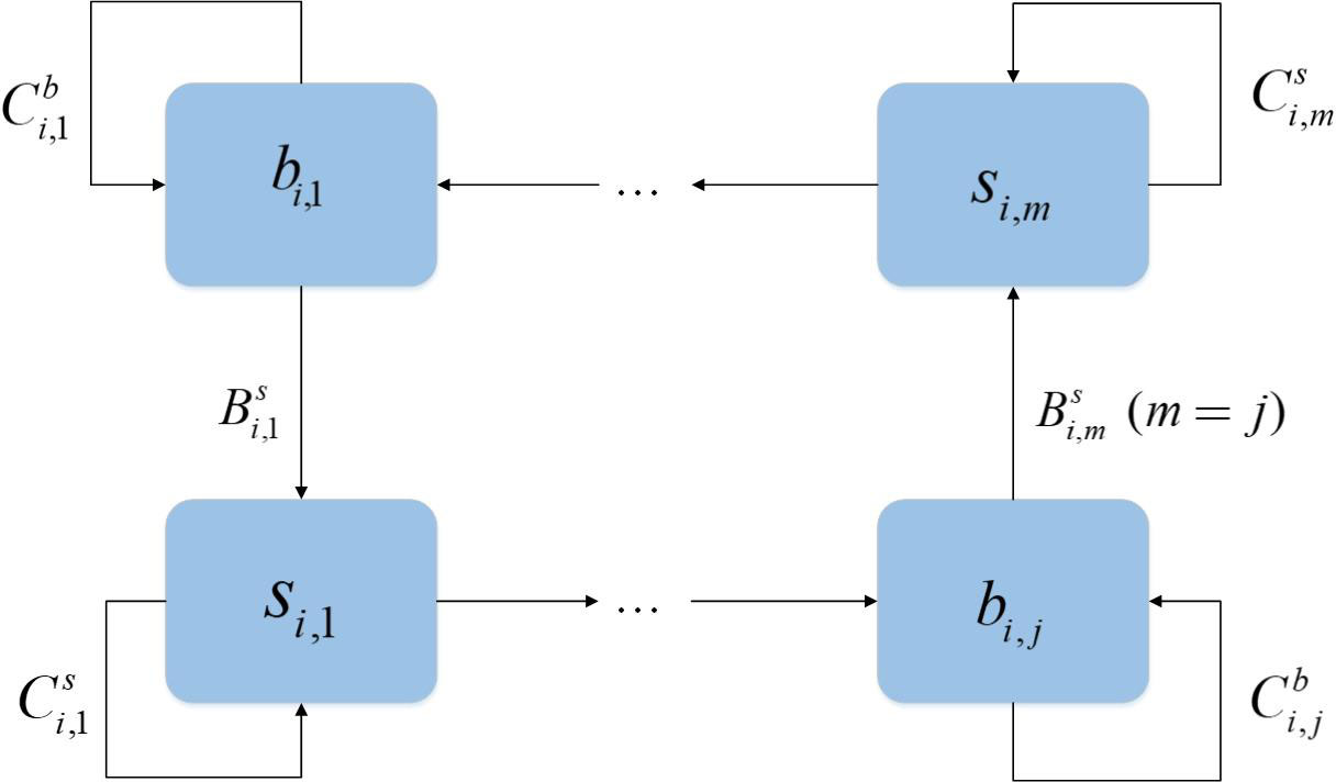
Figure 1 FSM module of liner shipping system.
A liner shipping schedule is a plan that combines time and space factors. Ships serving a certain shipping route are required to reach the corresponding port within the specified period. The importance of schedule reliability is reflected in two ways: (a) Container shipping is a key link in international cargo transportation. A liner shipping schedule provides an important basis for planning by other participants in the global supply chain, such as shippers, inland carriers, and marine container terminal (MCT) operators; therefore, any schedule delays would affect the subsequent logistics chain. (b) Schedule reliability reflects the service level a shipping line can achieve for customers; therefore, maintaining high levels of schedule reliability is beneficial for improving customer satisfaction and gaining competitive advantages.
Schedules published by shipping lines contain estimated times of arrival (ETA) and departure (ETD) for all ports they serve. In the liner shipping schedule, ETA and ETD are sequences of days, meaning that ships have to arrive or leave a port on a certain date, with the exact time (hours) not announced. For example, if the ETA for a certain port is 10, then the ship is supposed to arrive at the port within the period from 00:00 to 24:00 on the 10th day after the voyage starts—there is no requirement regarding the exact time (hours) of arrival. Such a practice allows some schedule flexibility.
However, at an operational level, more detailed instructions for arrivals and departures should be made; therefore, the ETA needs to be accurate to hours. An accurate ETA is key to the coordination between ships and MCT operators (Tao et al., 2023). As such, we transform the schedule into a series of position–time coordinates to obtain a tractable reference trajectory—the time series is in hours and the ships have reference positions at any instant.
In the voyage, the estimated time of arrival and departure of ship at port (denoted separately by and ) can be calculated by predetermined service speed (knots), estimated average port handling efficiency (TEU/hour), and estimated due quantities of containers to be handled (TEU). Then, and are set as relay points; therefore, we can derive all the position–time coordinates. Algorithm 1 shows the detailed process for generating the reference trajectories. We minimized the difference between the reference trajectories and the ships’ actual trajectories, which is called a tracking error, using a receding horizon scheme in Section 2.3 so that the ships follow the reference trajectories.
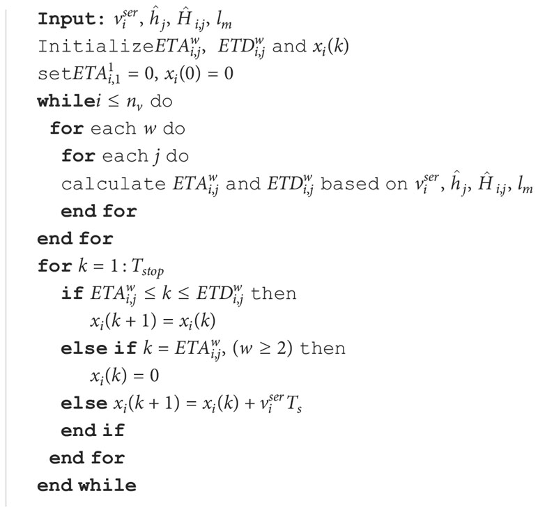
Algorithm 1 Reference trajectory generator.
Minimizing fuel consumption and carbon emissions are additional objectives when operating the liner shipping system in an energy-efficient way. Therefore, we calculate a formula for fuel consumption and carbon emissions as follows:
where is the indicated power (kW) of ship ; is the ship’s deadweight tonnage (DWT); is the admiralty coefficient; is the fuel consumption per unit time (t/h); and are the fuel consumption (t) and carbon emissions (t) in the time period ; and is the conversion factor between fuel consumption and emissions.
For calculation convenience, we transformed the fuel consumption and carbon emissions into linear expressions of speed. We used the cubic root of fuel consumption and carbon emissions as performance indicators of ship energy efficiency. The formulas are as follows:
The EEXI standard is introduced in the 2021 Marine Environmental Protection Committee meeting MEPC76, which acts as an expansion of the Energy Efficiency Design Index (EEDI) and covers existing ships. The attained EEXI for ships in liner shipping lines should be calculated and meet the required EEXI (IMO, 2022). Our calculation formulas for attained EEXI are as follows:
For ship ,
where is the required EEXI (), is the reference line of EEDI (), and is the attained EEXI (). is the reduction factor and is the safety margin, which are decided by the shipping lines themselves. is the service speed under the EEXI draft. is the correction factor and its value is 1. and are the carbon emissions of the main and auxiliary engines (); is the emissions of the shaft generator (); and and are the carbon emissions reduced by the innovative energy efficient devices in the auxiliary and main engines (). Our calculation formulas for the carbon emissions of various devices are as follows:
is the effective power of the main engine (kW), which is 75% of the maximum continuous rating (MCR); is the auxiliary engine power; , , and are the effective power of the shaft motor, and auxiliary and main engine power reductions due to energy efficient technology. and are correction factors and . and are the carbon converting factors; furthermore, here, we assume .
If the ship’s attained EEXI cannot meet the EEXI standard then adjusting measures should be carried out for EEXI compliance. Among various EEXI improvement solutions, EPL has been proven the most common choice by shipowners due to its effectiveness and economic feasibility. Therefore, our solution is to apply engine power limitation (EPL) to improve the ship’s EEXI.
Using the DHA model in Section 2.1 as the system plant, we created a DHA-DMPC framework, which is depicted in Figure 2. There is a local controller on each ship in the liner shipping fleet. The prediction model in the local MPC controller is a hybrid dynamical model built analogously to the DHA model from Section 2.1. We present the prediction model as follows:
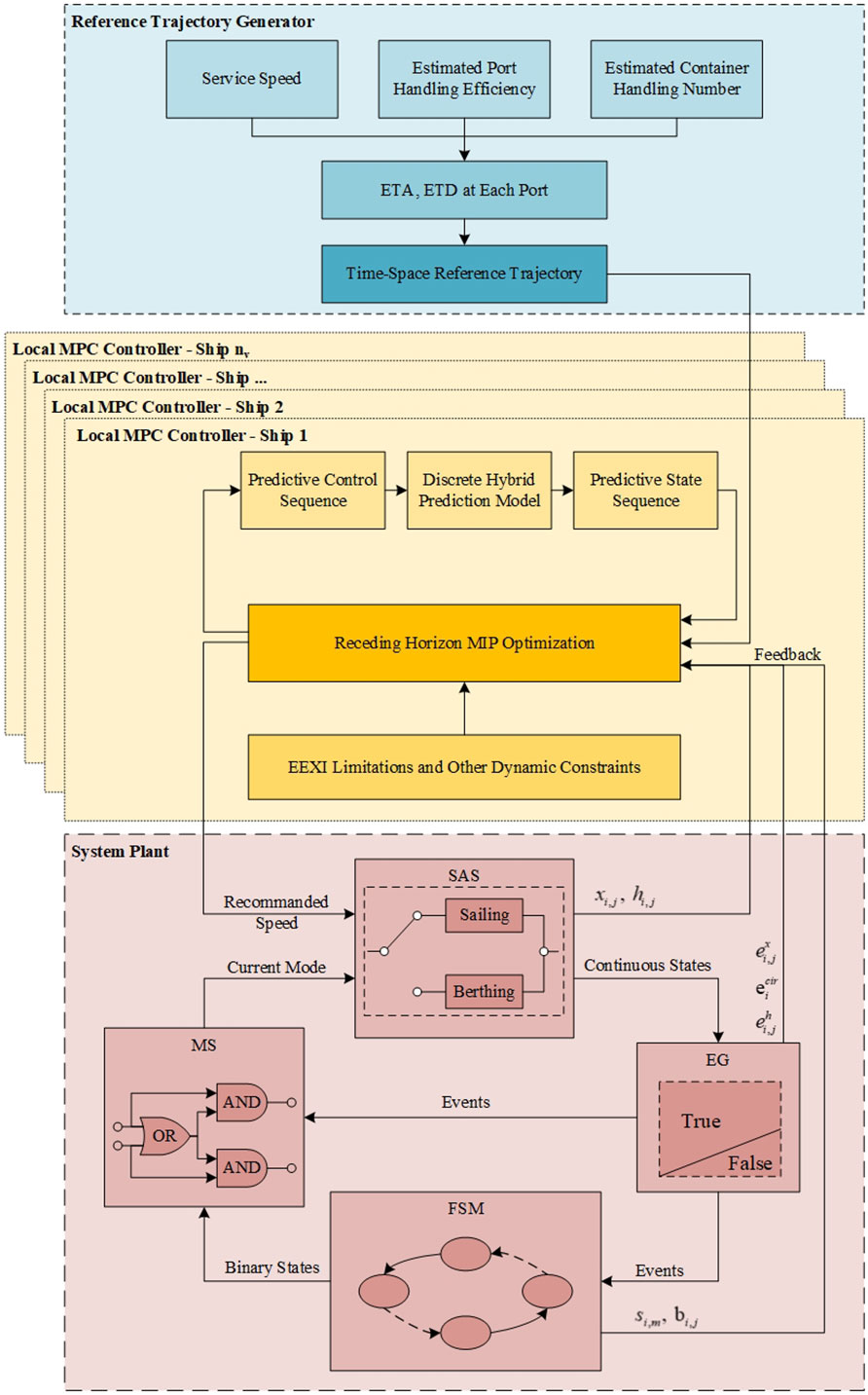
Figure 2 DHA-DMPC framework.
where (29) is analogous to the switched affine system in (1) and (2); , , and are the corresponding coefficients in mode M; the continuous state vector consists of the ship’s position at instant and handled container quantities at port ; the control vector contains the ship’s sailing speed at instant k; and the disturbance vector contains the port handling efficiency and due quantities of containers to be handled at port . Formula (30) is analogous to the event generator in (3)-(5); event vector consists of (the ship reaches port and container handling at port finishes) and (the ship accomplishes a round-circle voyage); and denotes the condition that triggers various events. Formula (31) is analogous to the mode selector in (6)-(8); the mode vector contains the sailing, berthing, and reset modes; the binary state vector consists of (the ship is sailing on leg ) and (the ship is berthing at port ); and represents the Boolean operation between the binary variables. Formula (32) is analogous to the finite state machine in (9)-(14); furthermore, in addition to those events in (30), event vector in (32) also consists of (the ship begins to sailing on leg ), (the ship is still sailing on leg ), (the ship begins to berth at port ), and (the ship is still berthing at port ); and represents the Boolean function, which consists of logical rules in the FSM module. Unlike the system plant, which includes all the ships in the fleet, the prediction model only considers a single ship; therefore, it involves fewer binary variables compared with the system plant and, thus, its computation capacity is much lower. This decentralized arrangement increases the computing speed of a local controller and enables real-time optimization of the ships’ speed (Negenborn and Maestre, 2014; Zheng et al., 2017; Wang et al., 2020).
Formula (33) is the optimization model in the DMPC controller, which considers minimizing tracking errors, fuel consumption, and carbon emissions as objectives. , , and are the weights of the three performance indicators (, ). The control variable is the sailing speed of each ship. We executed (33) using a receding horizon method to compensate for the uncertainties in the disturbances; moreover, binary variables are involved, such as the binary state variables and events in (30)-(32). Therefore, (33) is a mixed integer programming (MIP) problem.
In the receding horizon scheme, the prediction models predict future states in the prediction horizon after observing the current states; then, they calculate the tracking errors, resulting in every local controller computing the MIP optimization problem in (33) to obtain the control sequence in the control horizon. At each step, only the first element of the control sequence is implemented and the rest are ignored. Then, a new control sequence is obtained in the next step. We repeatedly execute this operation to realize online rolling optimization (Algorithm 2).
subject to
for ; :
initial states , , , ;
predictive model dynamics (29), (30), (31), (32);
EEXI limitations (22);
.
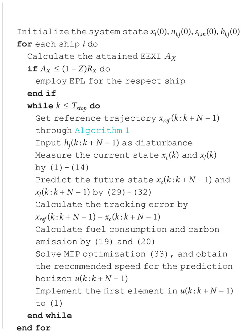
Algorithm 2 DHA-DMPC simulation..
We carried out a series of comparison studies to confirm the effectiveness of the suggested DHA-DMPC controller. In addition to the reference trajectory generated by Algorithm 1, we considered another reference trajectory to explore the performance of the controller. We introduce this new reference trajectory in Section 3.1.2. Furthermore, we expanded the EEXI standard into four phases with progressively higher reduction factors. We performed a sensitivity analysis to explore the impact of different carbon policies on liner shipping operations.
Various types of liner shipping routes exist, such as end-to-end, pendulum, and circular services (Notteboom, 2004). We choose the classical circular service for our case study, which is commonly used in practical liner shipping route design. Figure 3A shows the actual shipping route layout, and Table 1 displays the route’s parameters. The route can be abstracted as a concept of the circular voyage shown in Figure 3B, which means the ship visits a fixed port rotation on a pre-published schedule repeatedly. This route is served by four ships, and we assume that the fleet consists of four sister ships with the same technical conditions. Our calculations and solutions to improve the ships’ EEXI are shown in Section 3.1.3. All the data on shipping routes and sample ships are provided by CU Lines. The simulation period is the time for the fleet to accomplish two circle voyages, which is 1050 steps. The sampling time is 1h; furthermore, both the prediction and the control horizon are 10 steps. Table 2 shows the data from customer booking platform containing the due quantities of containers to be handled.
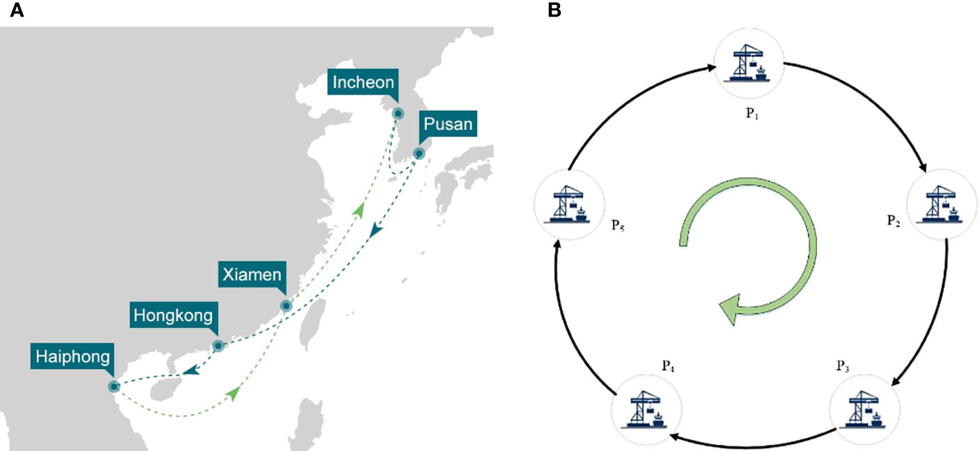
Figure 3 (A) real shipping route; (B) concept of circle voyage.
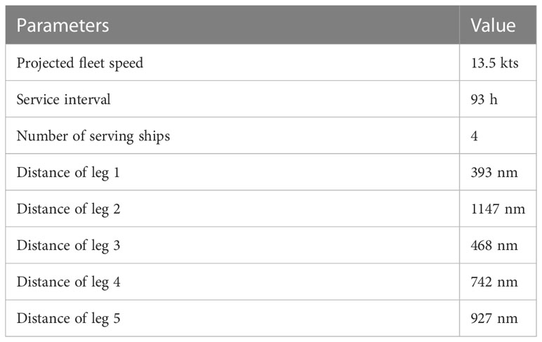
Table 1 Shipping route parameters.
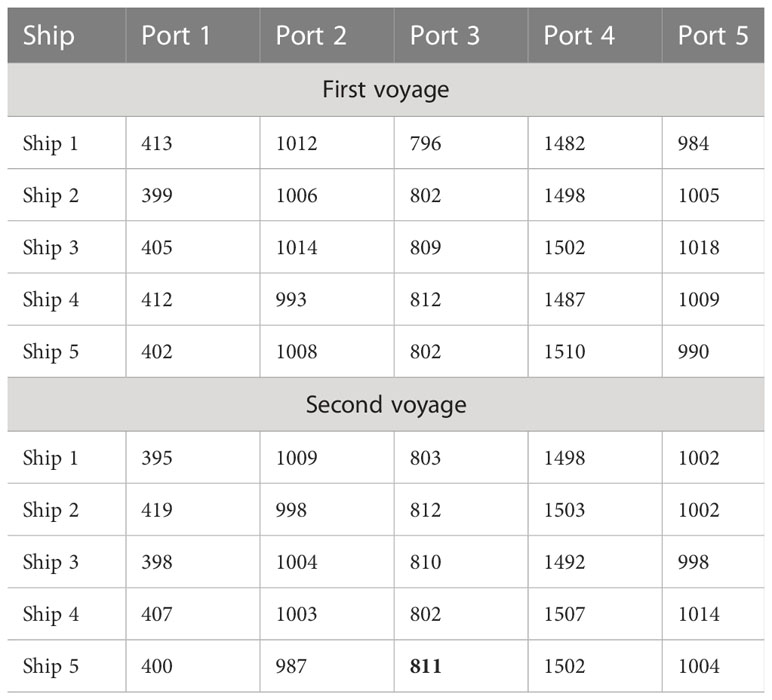
Table 2 Container handling numbers at different ports (TEU).
Table 3 displays the anticipated port handling efficiency used by shipping lines for tactical planning. The port handling efficiency is not the actual operation rate of the container terminal equipment; instead, it is an average handling efficiency rate, which is obtained by dividing the total number of containers handled by the total time that ships stay at port. However, in practice, port handling efficiency can fluctuate because of unpredictable factors, such as extreme weather, which makes loading and unloading operations difficult; port congestion, which increases the waiting time for ships to berth; or strikes, which result in low handling efficiency. Figure 4 shows the actual port handling efficiency during the simulation period, which we input into the optimization model as disturbances.
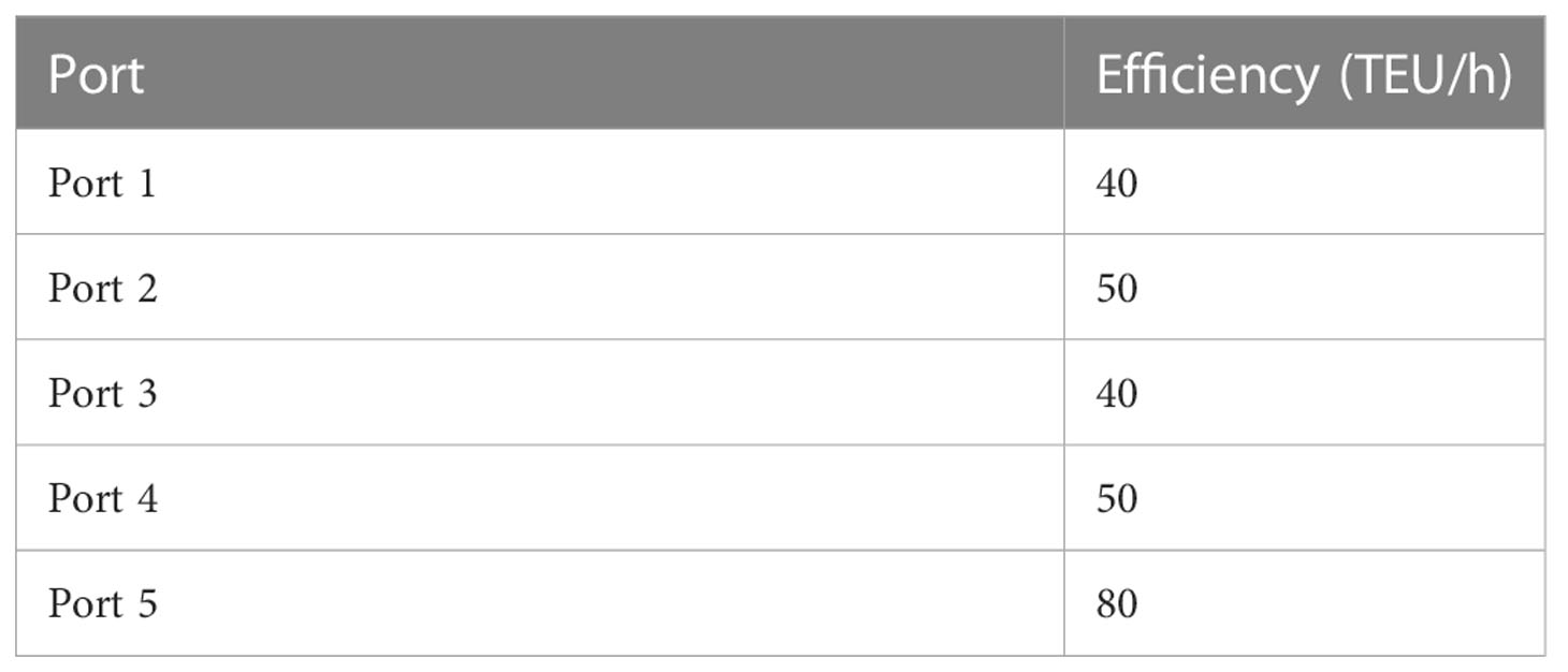
Table 3 Estimated port handling efficiency.
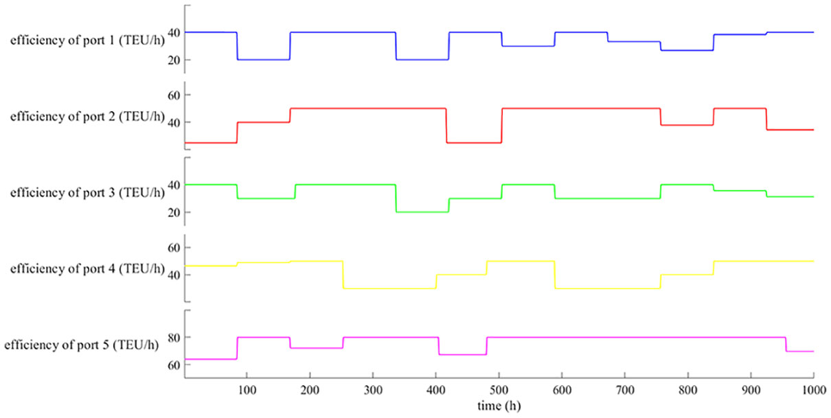
Figure 4 Real-time handling efficiency of each port.
We designed two reference trajectories and compared their performances: (a) Reference 1 ignores the berthing process. We set only as relay points to calculate the position–time coordinates. Algorithm 3 in Appendix A shows the detailed method to generate Reference 1. (b) Reference 2 considers the berthing process and is generated by Algorithm 1. Figure 5 illustrates the two reference trajectories.
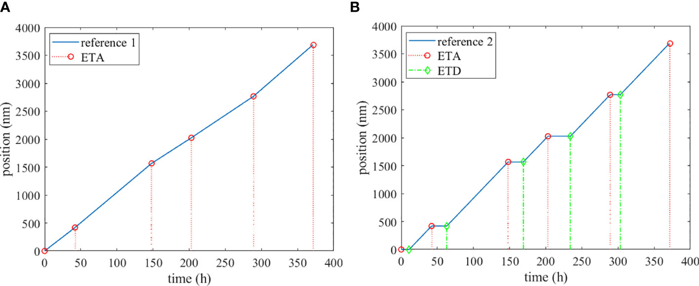
Figure 5 (A) Reference 1; (B) Reference 2.
Table 4 shows the ship’s parameters, which we used to calculate EEXI.
Table 4 Parameters for calculating EEXI.
The relationship between main engine power and speed can be described in a power–speed curve. The power–speed curve should be converted from the service draft to the EEXI draft. Figure 6 shows the transferred power–speed curve. The calculation equation is as follows:
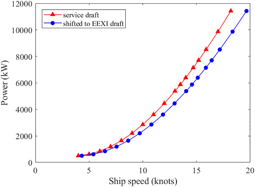
Figure 6 Power–speed curve.
where is the speed at EEXI draft, is the speed at service draft, is the displacement at service draft, and is the displacement at EEXI draft. For container ships, the service draft is the summer draft; furthermore, the EEXI draft is 70% summer draft.
The required EEXI/reference line is based on the below formula:
where , and .
The attained EEXI is 17.50 while the required EEXI with a 5% margin is 17.38 ; thus, the EPL has to be employed to limit the main engine power. We calculated the MCR after limitations as follows:
The limited MCR is 10787.9 kW, and the maximum speed under this limited MCR is 18 knots.
We created four scenarios to evaluate the controller’s effectiveness and assess how the two reference trajectories performed: (a) the ideal scenario, where the port handling efficiency retains the anticipated value throughout the simulation period; (b) the uncontrolled scenario; (c) the controlled scenario with Reference 1; and (d) the controlled scenario with Reference 2. Figure 7 shows the ships’ actual trajectories in the four scenarios, and the raw data are collected in Appendix B. Figure 7B shows that port delays and schedule disruptions are caused by uncertain port handling efficiency when no control actions are implemented. The intervals between the trajectory of ship 4 in its second voyage and that of ship 1 in the first voyage are larger compared to Figure 7A; in the second voyage, the trajectory of ship 3 is quite close to that of ship 4, and a bunching phenomenon (two ships stay at the same port at the same time) nearly happens at port 4. Figures 7C, D show the controlled results. We found that ships’ trajectories can be adjusted in time when a port delay happens to keep a steady ship delivery frequency.
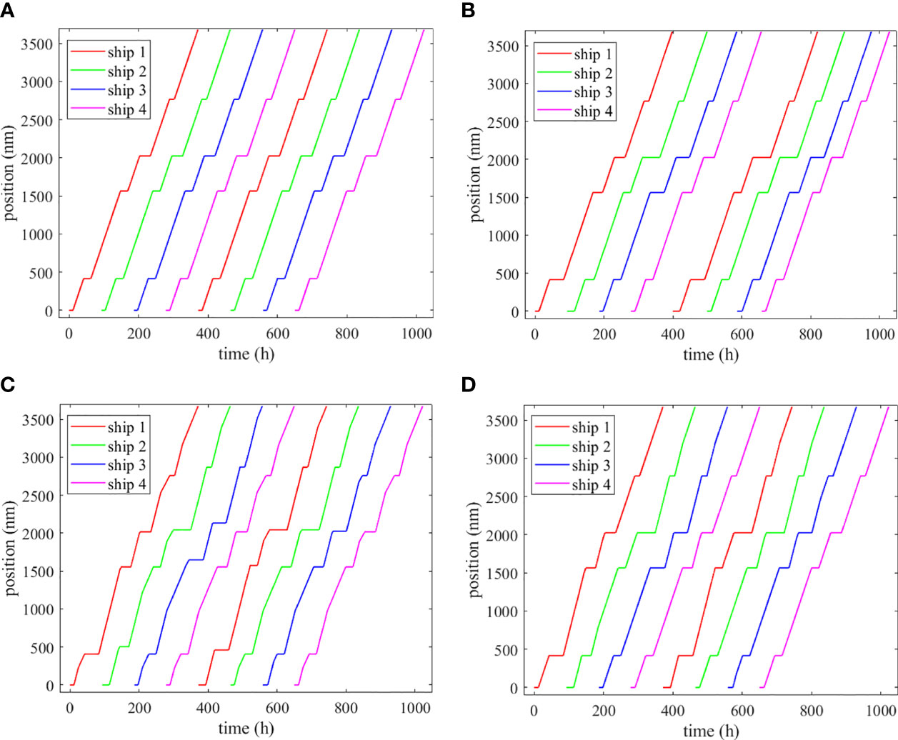
Figure 7 (A) Ideal trajectory; (B) uncontrolled; (C) controlled with Reference 1; (D) controlled with Reference 2.
Figures 8, 9 display the real-time sailing speed throughout each ship’s simulation period. The controller can increase the ship’s sailing speed with either reference trajectory whenever a delay is detected. We discovered differences between the performances of the two reference trajectories by comparing Figures 8, 9. After the delay is offset by the ship’s speed-up strategy, the ship’s speed will be reduced and maintained at a level lower than the projected service speed when controlled with Reference 1; however, when controlled with Reference 2, the ship’s speed will be turned back to the service speed after the speed-up strategy ceases.
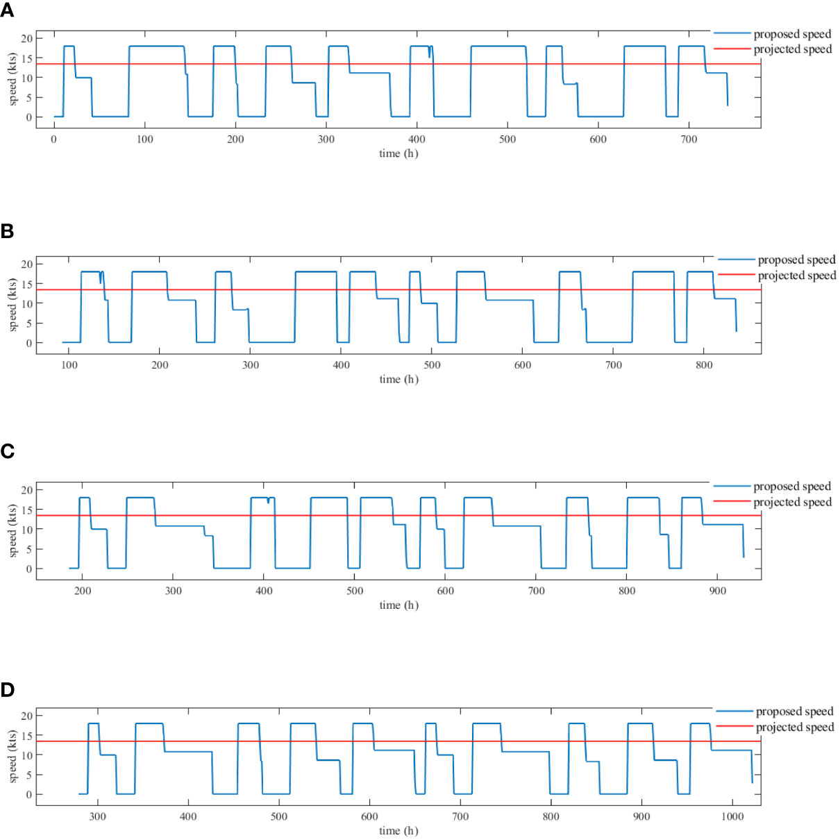
Figure 8 Speed of each ship under Reference 1: (A) ship 1; (B) ship 2; (C) ship 3; (D) ship 4.
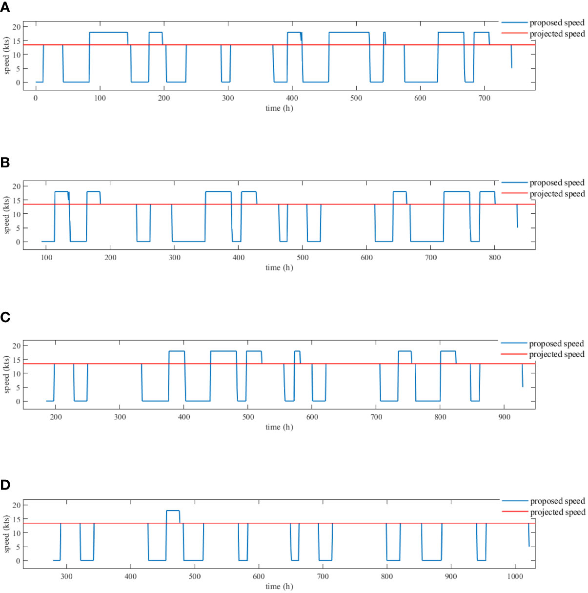
Figure 9 Speed of each ship under Reference 2: (A) ship 1; (B) ship 2; (C) ship 3; (D) ship 4.
Figure 10 demonstrates the delays (arrival time deviations) at each port of each ship under various scenarios. Figure 10 shows that compared with the uncontrolled scenario, the controller is capable of reducing port delays and maintaining high schedule reliability. When no control measures are taken, port delays cannot be corrected on time and will lead to progressively larger delays in subsequent ports. Take ship 1 as an example: Figures 10A, B demonstrate how port delays worsen over time. On the second voyage, the delay at port 5 reached 77 hours. Figures 10G, H depict the transferability of port delays. On the first voyage, ship 4 experienced a delay of 7 hours at port 4 due to fluctuations in handling efficiency at port 3. Thereafter, despite the normal efficiency of subsequent port operations, there were still 7-hour delays in each port. Instances of such delays will decrease (or even be eliminated) when control measures are taken, thus proving the effectiveness of our proposed DMPC controller.
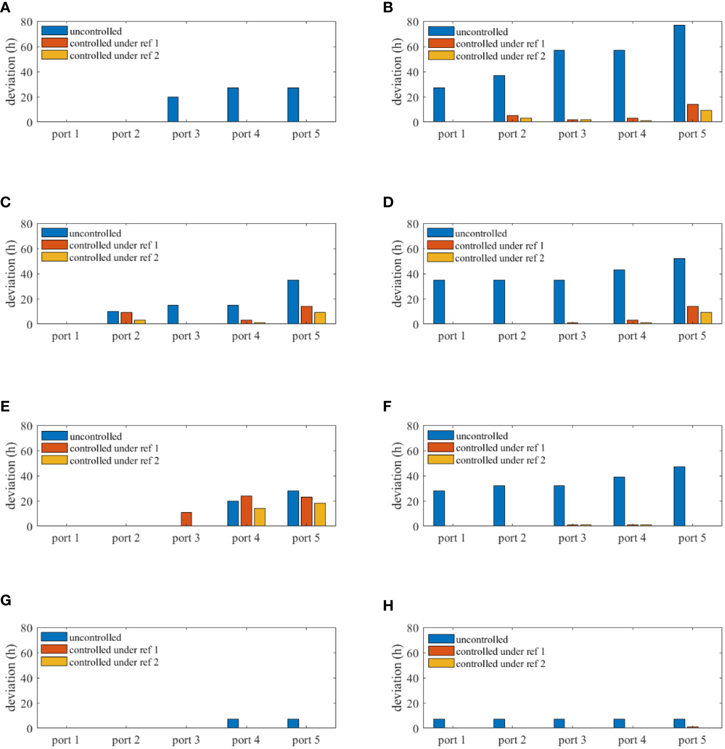
Figure 10 Arrival time deviations under different control methods at each port of: (A) ship 1 in the first voyage; (B) ship 1 in the second voyage; (C) ship 2 in the first voyage; (D) ship 2 in the second voyage; (E) ship 3 in the first voyage; (F) ship 3 in the second voyage; (G) ship 4 in the first voyage; (H) ship 4 in the second voyage.
Table 5 shows the total delay time, carbon emissions, and fuel consumption for various scenarios after two complete voyages; furthermore, we calculate the weighted comprehensive costs by the following formula:
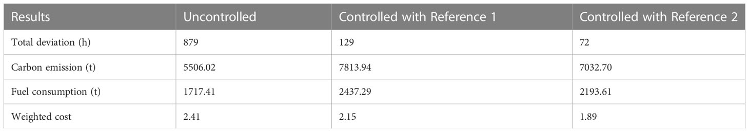
Table 5 Results under different control methods.
where is the standardized and weighted comprehensive costs under the scenario; is the total schedule deviations under the scenario; and and are the total carbon emissions and fuel consumption under the scenario, respectively. Our standardization operation divides each indicator by the maximum of all indicators under various scenarios, mapping the values of all indicators to the interval (Zhen et al., 2023). The weights of the indicators are , , and .
Table 5 shows that our proposed controller can effectively reduce port delays. The results also demonstrate the superiority of Reference 2 over 1. When the fleet is controlled with Reference 1, the total deviations is 14.68% of the result without control actions, while with Reference 2 the overall deviations only account for 8.20% of that without control. For fuel consumption and carbon emissions, the fleet consumes less fuel and produces fewer emissions due to the lower average speed. When control actions are involved, ships will speed up to the next port to catch the schedule at the cost of higher fuel consumption rates and more carbon emissions. Moreover, Reference 2 is superior to Reference 1 in terms of energy efficiency management. Carbon emissions and fuel consumption in a Reference-1 scenario are 10% less than with Reference 2. Such a result can be explained by the real-time speed displayed in Figures 8, 9. Compared with Reference 1, speed with Reference 2 is smoother. Speed with Reference 1 fluctuates too frequently and sharply, resulting in increased fuel consumption and carbon emissions. Our proposed controller can effectively reduce comprehensive and combined costs. Comprehensive cost under Reference 1 is 10.79% less than that without control, and the combined cost under Reference 2 is 21.58% less, which is twice as much as the former. However, on balance, Reference 2 achieves the best final result.
We designed further experiments to expand the EEXI standard into four phases and explore the impact of carbon emission policies on liner shipping operations. Each phase adopted stricter regulations than the previous, i.e., the reduction factor increases phase by phase. The reduction factors of the four phases are: 20%, 25, 30%, and 40%. The EEXI margin is 5%. Because we proved the superiority of Reference 2 in Section 3.2, we adopted Reference 2 as the reference trajectory for the DMPC controller. Table 6 shows EPL solutions applied to the sample ship in different phases.

Table 6 Limited MCR under different EEXI margins.
Figure 11 and Table 7 show our sensitive analysis results. Port delay statistics (Figure 11) show that a stricter EEXI standard produces higher schedule deviations. In Phase 4, due to the main engine’s excessive power limitations, the upper-speed limit drastically reduced—the maximum speed is only 14 knots, which is only 0.5 knots higher than the projected service speed. The speed-up method’s potency in reducing schedule delays is greatly diminished; therefore, the port delays cannot be dealt with effectively. Figure 11 shows that the transferability of port delays happened again in Phase 4, indicating that a speed-up strategy failed in eliminating port delays. Table 7 shows performance indicators with progressive emission limits in each phase. The maximum speed a ship can reach is gradually reduced, with carbon emissions and fuel consumption decreasing due to the overall reduction in sailing speed, eventually leading to higher overall costs due to the expansion of delays. In Phase 2, there is a small increase in port delays; however, overall carbon emissions and fuel consumption are reduced, making the overall cost comparable to Phase 1. Despite this, the comprehensive costs of Phase 3 and 4 are considerably increased due to excessive delays.
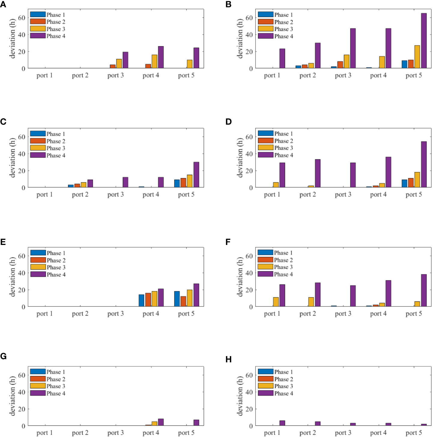
Figure 11 Arrival time deviations in different phases at each port of (A) ship 1 in the first voyage; (B) ship 1 in the second voyage; (C) ship 2 in the first voyage; (D) ship 2 in the second voyage; (E) ship 3 in the first voyage; (F) ship 3 in the second voyage; (G) ship 4 in the first voyage; (H) ship 4 in the second voyage.
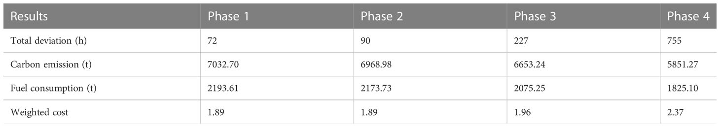
Table 7 Results in different phases.
In our paper, we investigated how liner shipping lines can maintain schedule reliability while reducing carbon emissions and fuel consumption through real-time speed optimization under the uncertainty of port handling efficiency and the need to meet EEXI standards. Firstly, we established a DHA model to describe the hybrid dynamic characteristics of the liner shipping system. Then, we constructed a prediction model using the DMPC framework by analogy with the previously established DHA model. Next, we designed a DMPC controller based on the receding horizon optimization method. In the DMPC framework, the schedule is converted into tractable position–time coordinates; furthermore, we considered minimizing tracking errors, carbon emissions, and fuel consumption as optimization objectives, and converted the EEXI specification into constraints by using the EPL solution. We adjusted the ships’ speeds by an online rolling optimization method to compensate for the impact caused by uncertain port handling efficiency. Our experiments verify the effectiveness of our proposed DHA-DMPC controller. Our sensibility analysis revealed that the rolling optimization method considerably reduces fleet port delays; however, these improvements come at the expense of consuming more fuel and emitting more carbon emissions. Therefore, the liner company must maximize the overall benefits by weighing the relationship between schedule reliability and energy efficiency.
Finally, we present our conclusions from analyzing our experimental results regarding decision making for liner shipping lines:
(a) Liner shipping operations are vulnerable to operational uncertainties in ports, and it is impossible to accurately predict port handling efficiency. As a result, the service speed determined in tactical planning often loses its optimality during operations. When a port delay occurs, if the ship continues to sail at the service speed, the delay will be worsened because of a lack of timely adjustment measures. This will eventually not only reduce the service level of the shipping company but also disrupt the supply chain by affecting the coordination of ships and MCT operators. Therefore, real-time ship speed management is essential. The real-time adjustment of vessel speeds enables robust fleet operation, allowing management to cope with unexpected external conditions and maintain high service levels while effectively controlling overall fleet fuel consumption and carbon emissions;
(b) Table 6 shows the main engine power limitations of the sample ship for various EEXI phases, and we can infer that under strict emission regulations, the fleet’s technology performance will be constrained, reducing the maximum speeds that the ships can reach. The ability to improve schedule reliability and energy efficiency by adjusting operation speeds will be considerably constrained if the maximum speed of the ship is further restricted. Liner shipping lines may consider adding more ships to the route or improving the fleet’s technical efficiency to maintain a steady schedule;
(c) Table 7 reveals that maintaining high schedule reliability by taking control actions will finally lead to more fuel consumption and carbon emissions. Liner shipping lines should balance the trade-off between ships’ fuel consumption, carbon emissions, and schedule reliability by implementing appropriate speed-reduction strategies. Another recommendation is to use sustainable energy so that the ship can significantly reduce its emissions while traveling at the same speed. As a result, the shipping lines can maintain a steady and competitive schedule while traveling faster and emitting less carbon dioxide.
The original contributions presented in the study are included in the article/supplementary material. Further inquiries can be directed to the corresponding author.
JZ and QZ contributed to conception and design of the study. JZ organized the database. CM performed the statistical analysis. JZ and CM wrote the first draft of the manuscript. JZ, CM, and QZ wrote sections of the manuscript. All authors contributed to the article and approved the submitted version.
The research is supported by the International Cooperation Project (21160710800) of Shanghai Science and Technology Committee.
The authors declare that the research was conducted in the absence of any commercial or financial relationships that could be construed as a potential conflict of interest.
All claims expressed in this article are solely those of the authors and do not necessarily represent those of their affiliated organizations, or those of the publisher, the editors and the reviewers. Any product that may be evaluated in this article, or claim that may be made by its manufacturer, is not guaranteed or endorsed by the publisher.
An K., Lo H. K. (2016). Two-phase stochastic program for transit network design under demand uncertainty. Transport. Res. Part B: Methodol. 84, 157–181. doi: 10.1016/j.trb.2015.12.009
Aydin N., Lee H., Mansouri S. A. (2017). Speed optimization and bunkering in liner shipping in the presence of uncertain service times and time windows at ports. Eur. J. Operational Res. 259 (1), 143–154. doi: 10.1016/j.ejor.2016.10.002
Bemporad A., Morari M. (1999). Control of systems integrating logic, dynamics, and constraints. Automatica 35 (3), 407–427. doi: 10.1016/S0005-1098(98)00178-2
Brouer B. D., Karsten C. V., Pisinger D. (2017). Optimization in liner shipping. 4OR 15 (1), 1–35. doi: 10.1007/s10288-017-0342-6
Chen J., Ye J., Liu A., Fei Y., Wan Z., Huang X. (2022). Robust optimization of liner shipping alliance fleet scheduling with consideration of sulfur emission restrictions and slot exchange. Ann. Operations Res., 1–31. doi: 10.1007/s10479-022-04590-x
Dunn C., Theriault J., Hickmott L., Claridge D. (2021). Slower ship speed in the Bahamas due to COVID-19 produces a dramatic reduction in ocean sound levels. Front. Mar. Sci. 8, 673565. doi: 10.3389/fmars.2021.673565
Fagerholt K., Laporte G., Norstad I. (2010). Reducing fuel emissions by optimizing speed on shipping routes. J. Operational Res. Soc. 61 (3), 523–529. doi: 10.1057/jors.2009.77
Guericke S., Tierney K. (2015). Liner shipping cargo allocation with service levels and speed optimization. Transport. Res. Part E: Logistics Transport. Rev. 84, 40–60. doi: 10.1016/j.tre.2015.10.002
Huotari J., Manderbacka T., Ritari A., Tammi K. (2021). Convex optimisation model for ship speed profile: Optimisation under fixed schedule. J. Mar. Sci. Eng. 9 (7), 730. doi: 10.3390/jmse9070730
IMO (2022). “Resolution MEPC.350(78),” in 2022 guidelines on the method of calculation of the attained energy efficiency existing ship index (EEXI) (London: IMO).
Jimenez V. J., Kim H., Munim Z. H. (2022). A review of ship energy efficiency research and directions towards emission reduction in the maritime industry. J. Clean. Prod. 366, 132888. doi: 10.1016/j.jclepro.2022.132888
Karsten C. V., Brouer B. D., Pisinger D. (2017). Competitive liner shipping network design. Comput. Operations Res. 87, 125–136. doi: 10.1016/j.cor.2017.05.018
Leaper R. (2019). The role of slower vessel speeds in reducing greenhouse gas emissions, underwater noise and collision risk to whales. Front. Mar. Sci. 6, 505. doi: 10.3389/fmars.2019.00505
Lee H., Aydin N., Choi Y., Lekhavat S., Irani Z. (2018). A decision support system for vessel speed decision in maritime logistics using weather archive big data. Comput. Operations Res. 98, 330–342. doi: 10.1016/j.cor.2017.06.005
Li X., Sun B., Zhao Q., Li Y., Shen Z., Du W., et al. (2018). Model of speed optimization of oil tanker with irregular winds and waves for given route. Ocean Eng. 164, 628–639. doi: 10.1016/j.oceaneng.2018.07.009
Liu M., Liu X., Chu F., Zhu M., Zheng F. (2020). Liner ship bunkering and sailing speed planning with uncertain demand. Comput. Appl. Math. 39 (1), 1–23. doi: 10.1007/s40314-019-0994-2
Meng Q., Wang S., Andersson H., Thun K. (2014). Containership routing and scheduling in liner shipping: overview and future research directions. Transport. Sci. 48 (2), 265–280. doi: 10.1287/trsc.2013.0461
Negenborn R. R., Maestre J. M. (2014). Distributed model predictive control: An overview and roadmap of future research opportunities. IEEE Control Syst. Mag. 34 (4), 87–97. doi: 10.1109/MCS.2014.2320397
Notteboom T. E. (2004). A carrier's perspective on container network configuration at sea and on land. J. Int. logistics trade 1 (2), 65–87. doi: 10.24006/jilt.2004.1.2.65
Notteboom T. E. (2006). The time factor in liner shipping services. Maritime Econ Logistics 8 (1), 19–39. doi: 10.1057/palgrave.mel.9100148
Pasha J., Dulebenets M. A., Fathollahi-Fard A. M., Tian G., Lau Y. Y., Singh P., et al. (2021). An integrated optimization method for tactical-level planning in liner shipping with heterogeneous ship fleet and environmental considerations. Adv. Eng. Inf. 48, 101299. doi: 10.1016/j.aei.2021.101299
Perera L. P., Mo B. (2016). Emission control based energy efficiency measures in ship operations. Appl. Ocean Res. 60, 29–46. doi: 10.1016/j.apor.2016.08.006
Psaraftis H. N., Kontovas C. A. (2014). Ship speed optimization: Concepts, models and combined speed-routing scenarios. Transport. Res. Part C: Emerging Technol. 44, 52–69. doi: 10.1016/j.trc.2014.03.001
Qi X., Song D. P. (2012). Minimizing fuel emissions by optimizing vessel schedules in liner shipping with uncertain port times. Transport. Res. Part E: Logistics Transport. Rev. 48 (4), 863–880. doi: 10.1016/j.tre.2012.02.001
Sheng X., Chew E. P., Lee L. H. (2015). (s, s) policy model for liner shipping refueling and sailing speed optimization problem. Transport. Res. Part E: Logistics Transport. Rev. 76, 76–92. doi: 10.1016/j.tre.2014.12.001
Sirmatel I. I., Geroliminis N. (2018). Mixed logical dynamical modeling and hybrid model predictive control of public transport operations. Transport. Res. Part B: Methodol. 114, 325–345. doi: 10.1016/j.trb.2018.06.009
Tan Z., Wang Y., Meng Q., Liu Z. (2018). Joint ship schedule design and sailing speed optimization for a single inland shipping service with uncertain dam transit time. Transport. Sci. 52 (6), 1570–1588. doi: 10.1287/trsc.2017.0808
Tao Y., Zhang S., Lin C., Lai X. (2023). A bi-objective optimization for integrated truck operation and storage allocation considering traffic congestion in container terminals. Ocean Coast. Manage. 232, 106417. doi: 10.1016/j.ocecoaman.2022.106417
Tzortzis G., Sakalis G. (2021). A dynamic ship speed optimization method with time horizon segmentation. Ocean Eng. 226, 108840. doi: 10.1016/j.oceaneng.2021.108840
Wang K., Li J., Yan X., Huang L., Jiang X., Yuan Y., et al. (2020). A novel bi-level distributed dynamic optimization method of ship fleets energy consumption. Ocean Eng. 197, 106802. doi: 10.1016/j.oceaneng.2019.106802
Wang S., Meng Q. (2012a). Robust schedule design for liner shipping services. Transport. Res. Part E: Logistics Transport. Rev. 48 (6), 1093–1106. doi: 10.1016/j.tre.2012.04.007
Wang S., Meng Q. (2012b). Sailing speed optimization for container ships in a liner shipping network. Transport. Res. Part E: Logistics Transport. Rev. 48 (3), 701–714. doi: 10.1016/j.tre.2011.12.003
Wang K., Yan X., Yuan Y., Jiang X., Lin X., Negenborn R. R. (2018). Dynamic optimization of ship energy efficiency considering time-varying environmental factors. Transport. Res. Part D: Transport Environ. 62, 685–698. doi: 10.1016/j.trd.2018.04.005
Wang K., Yan X., Yuan Y., Jiang X., Lodewijks G., Negenborn R.R., et al (2021). Study on route division for ship energy efficiency optimization based on big environment data. In Proceedings of the 4th International Conference on Transportation Information and Safety (ICTIS) (Banff, AB, Canada), 111-116. doi: 10.1109/ICTIS.2017.8047752
Wen M., Pacino D., Kontovas C. A., Psaraftis H. N. (2017). A multiple ship routing and speed optimization problem under time, cost and environmental objectives. Transport. Res. Part D: Transport Environ. 52, 303–321. doi: 10.1016/j.trd.2017.03.009
Xia J., Li K. X., Ma H., Xu Z. (2015). Joint planning of fleet deployment, speed optimization, and cargo allocation for liner shipping. Transport. Sci. 49 (4), 922–938. doi: 10.1287/trsc.2015.0625
Zhen R., Lv P., Shi Z., Chen G. (2023). A novel fuzzy multi-factor navigational risk assessment method for ship route optimization in costal offshore wind farm waters. Ocean Coast. Manage. 232, 106428. doi: 10.1016/j.ocecoaman.2022.106428
Zheng J., Ma Y., Ji X., Chen J. (2021). Is the weekly service frequency constraint tight when optimizing ship speeds and fleet size for a liner shipping service? Ocean Coast. Manage. 212, 105815. doi: 10.1016/j.ocecoaman.2021.105815
Zheng H., Negenborn R. R., Lodewijks G. (2017). Closed-loop scheduling and control of waterborne AGVs for energy-efficient inter terminal transport. Transport. Res. Part E: Logistics Transport. Rev. 105, 261–278. doi: 10.1016/j.tre.2016.07.010

Algorithm 3 reference trajectory generator ignoring berthing process..
Table 8 ETA/ETD in the ideal situation.
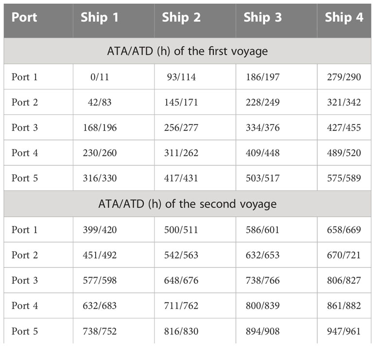
Table 9 ATA/ATD (Actual time of arrival/departure) in an uncontrolled scenario.
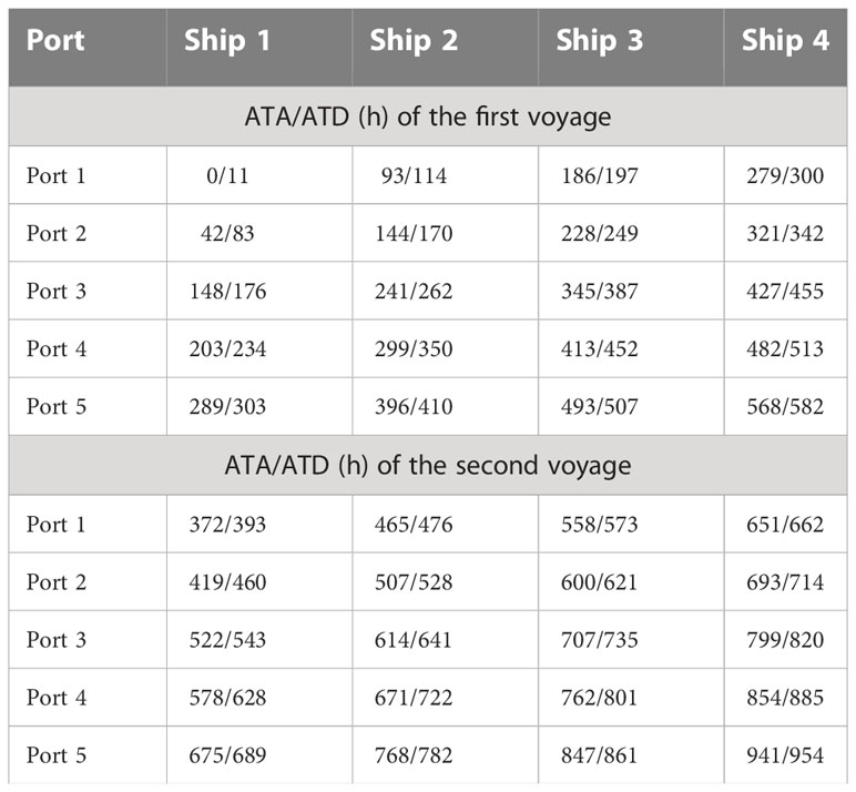
Table 10 ATA/ATD in the scenario under reference 1.
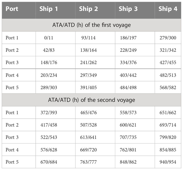
Table 11 ATA/ATD in the scenario under reference 2.
Keywords: liner shipping, speed optimization, model predictive control, discrete hybrid automaton, Energy Efficiency Existing Ship Index (EEXI)
Citation: Zheng J, Mao C and Zhang Q (2023) Hybrid dynamic modeling and receding horizon speed optimization for liner shipping operations from schedule reliability and energy efficiency perspectives. Front. Mar. Sci. 10:1095283. doi: 10.3389/fmars.2023.1095283
Received: 11 November 2022; Accepted: 09 March 2023;
Published: 21 March 2023.
Edited by:
Jihong Chen, Shenzhen University, ChinaReviewed by:
Kang Chen, Dalian Maritime University, ChinaCopyright © 2023 Zheng, Mao and Zhang. This is an open-access article distributed under the terms of the Creative Commons Attribution License (CC BY). The use, distribution or reproduction in other forums is permitted, provided the original author(s) and the copyright owner(s) are credited and that the original publication in this journal is cited, in accordance with accepted academic practice. No use, distribution or reproduction is permitted which does not comply with these terms.
*Correspondence: Qiang Zhang, cWlhbmd6aGFuZ0BzaG10dS5lZHUuY24=
Disclaimer: All claims expressed in this article are solely those of the authors and do not necessarily represent those of their affiliated organizations, or those of the publisher, the editors and the reviewers. Any product that may be evaluated in this article or claim that may be made by its manufacturer is not guaranteed or endorsed by the publisher.
Research integrity at Frontiers
Learn more about the work of our research integrity team to safeguard the quality of each article we publish.