Developing machine learning methods for automatic recognition of fishing vessel behaviour in the Scomber japonicus fisheries

Introduction: With a higher degree of automation, fishing vessels have gradually begun adopting a fishing monitoring method that combines human and electronic observers. However, the objective data of electronic monitoring systems (EMS) has not yet been fully applied in various fishing boat scenarios such as ship behavior recognition.

Methods: In order to make full use of EMS data and improve the accuracy of behaviors recognition of fishing vessels, the present study proposes applying popular deep learning technologies such as convolutional neural network, long short-term memory, and attention mechanism to Chub mackerel (Scomber japonicus) fishing vessel behaviors recognition. The operation process of Chub mackerel fishing vessels was divided into nine kinds of behaviors, such as “pulling nets”, “putting nets”, “fish pick”, “reprint”, etc. According to the characteristics of their fishing work, four networks with different convolutional layers were designed in the pre-experiment. And the feasibility of each network in behavior recognition of the fishing vessels was observed. The pre-experiment is optimized from the perspective of the data set and the network. From the standpoint of the data set, the size of the optimized data set is significantly reduced, and the original data characteristics are preserved as much as possible. From the perspective of the network, different combinations of pooling, long short-term memory(LSTM) network, and attention(including CBAM and SE) are added to the network, and their effects on training time and recognition effect are compared.

Results: The experimental results reveal that the deep learning methods have outstanding performance in behaviors recognition of fishing vessels. The LSTM and SE module combination produced the most apparent optimization effect on the network, and the optimized model can achieve an F1 score of 97.12% in the test set, surpassing the classic ResNet, VGGNet, and AlexNet.

Discussion: This research is of great significance to the management of intelligent fishery vessels and can promote the development of electronic monitoring systems for ships.

1 Introduction

Behaviors recognition of vessels is a very active topic in intelligent maritime navigation, which is of great significance for identifying potential risks of vessels and improving maritime traffic efficiency (Chen et al., 2020). Vessels behavior recognition algorithms have been widely used in marine traffic (Arguedas et al., 2017) and other aspects. However, due to the relatively low degree of informatization of fishing vessels, the current fishing vessel’s behavior recognition is still in its infancy. There are relatively few applications related to fishing vessels’ behavior recognition. In addition to its contribution to optimizing maritime traffic, the recognition of fishing vessel behavior is of unique significance (relative to commercial) for regulating fishing operations, reducing the cost of fisheries management, etc. Most applications in previous years were based on vessel position data, such as VMS(Vessel Monitoring System), to identify and predict vessel behavior. With the rapid development of electronic monitoring systems in recent years, more and more ships have installed electronic monitoring systems (Gilman et al., 2019). These electronic monitoring systems have become a powerful supplement or even a substitute for human observers as electronic observers. And the rich EMS data provides more robust data support for ship behavior recognition. Therefore, vessel behavior recognition can be divided into ship position-based and video-based from the data source.

Many positions and trajectory information has accumulated with satellite positioning technology’s wide application in ships. Faced with these massive amounts of information, scientific researchers and fishery production personnel hope to obtain practical knowledge. The rich positioning information reflects the position change process of the ship, which can reflect the operation characteristics of the ship in a period to a certain extent. Therefore, many studies on ship behavior recognition based on position data have sprung up in academia. Fishing vessel behavior identification is significant to safety production and fishery ecology. Therefore, studies on ship behavior recognition based on ship position data have emerged in an endless stream in recent years. Feng et al (Feng et al., 2019). used VMS data and BP neural network method to identify the fishing behavior of fishing boats. Variation trends of fishing boat angle and speed were selected as input parameters, and the accuracy of identifying fishing behavior reached 79%. Patroumpas K et al (Patroumpas et al., 2017). proposed a system for online monitoring of maritime activities based on AIS data and embedded a complex behavior recognition module. The behavior recognition module is mainly used to identify potential risks at sea. Sun et al (Sun et al., 2018). mine various motion patterns based on ship position data, which can be applied to ship behavior recognition. Although there are many studies on ship behavior based on ship position information, most of these studies focus on distinguishing whether a ship is fishing. In working, fishing boats may have many behaviors, and even different fishing methods will have different fishing behaviors. Simply dividing all fishing vessel activities into “fishing” and “other” is not enough to reflect the complete working process of fishing vessels.

In recent years, vessel behavior detection based on video data has been an emerging ship behavior recognition method. Video data mainly includes surveillance video data installed on the hull and public surveillance data nestled on the shore. Solano-Carrillo et al. The amount of information included in the video data is obviously far greater than that of the position data. The popularity of EMS helps to monitor the fishing process comprehensively and limit illegal fishing. However, the development of EMS is still in its infancy, and there is a lack of complete examples in the industry. A considerable part of EMS is still set for research (Solano-Carrillo et al., 2021). used marine surveillance camera data to detect anomalous behavior of ships using generative adversarial networks. Wang et al. (2022) proposed a 3D convolutional neural network method to detect the behavior of Acetes chinensis fishing boats and achieved an accuracy of 97.09% with EMS data. Cao et al. (2020) proposed a method of extracting ship features by combining a convolutional neural network and Zemike aiming at the problem of ship recognition in video images and the recognition accuracy rate for three types of ships reached 87%. The amount of information in the video data is more significant, and the recognition results are also more verifiable.

The EMS on fishing vessels has not yet formed a mature installation system, and the installation positions of cameras on different ships are also different. Therefore, exploratory research on vessel behavior identification based on EMS data can only be found on some specific fishing vessels. Chub mackerel Scomber japonicus (Hunter and Kimbrell, 1980) is a near-coastal pelagic migratory fish with phototaxis and vertical movement phenomenon. It is distributed in the Korean Peninsula, Japan, the Atlantic, and Mediterranean coasts, the southern coast of the Indian Ocean and Africa, the western coast of the Pacific Ocean from the Philippines to the Russian Far East, and the most northerly to the Gulf of Alaska in North America. In China, S. japonicus is found in the Yellow Sea, East China Sea, and South China Sea. Because of its good taste, Chub mackerel’ firm meat is sold fresh, pickled, canned, and refined into artificial butter. In addition, its liver is rich in vitamin A and can be used to make cod liver oil. Therefore, it has a high economic value. Chinese fishing vessels mainly fish for Chub mackerel resources utilizing light purse seine and light lift net. And the fishing vessel used in this research used the light lift net method. China’s Chub mackerel fishing vessel electronic monitoring system is gradually covered, but the use of its electronic monitoring system data is more petite.

The popularization of EMS is one of the important development directions of fishery monitoring in the future, so it is of great significance to identify ship behavior based on EMS data. In video and image recognition, the current common processing schemes include traditional computer vision processing schemes, support vector machine classification schemes (Hamdan, 2021), and convolutional neural network processing schemes (Rani et al., 2021). The convolutional neural network has the most excellent performance in video recognition tasks in various fields.

Therefore, this research transplants convolutional neural networks and popular deep learning methods into Chub mackerel EMS data processing, trying to provide an effective solution for EMS data processing. And the specific task of this research is to complete the behavior identification of a specific fishing vessel through the electronic monitoring data of the fishing vessel. The results of behavior recognition are used for further fishing vessel monitoring. The conclusions of this research can provide technical support for improving the standardization of fishing.

2 Data and methods

2.1 Data

All data used in the present study come from the EMS of the Chub mackerel fishing vessels of Zhoushan Xinhai Fishery Company in China(starting now referred to as Xinhai vessels). We collected 9000GB of EMS data from 10 of the above fishing vessels. EMS with specific specifications is equipped in Xinhai’s Chub mackerel fishing vessels. And each set of EMS includes seven cameras(Hikvision’s DS-2CE16F5P-IT3 camera). Seven sets of cameras are installed on the bow, stern, cabin, and other positions of Xinhai vessels to record different types of video data. The installation position of each camera on the hull is shown in Figure 1.

FIGURE 1

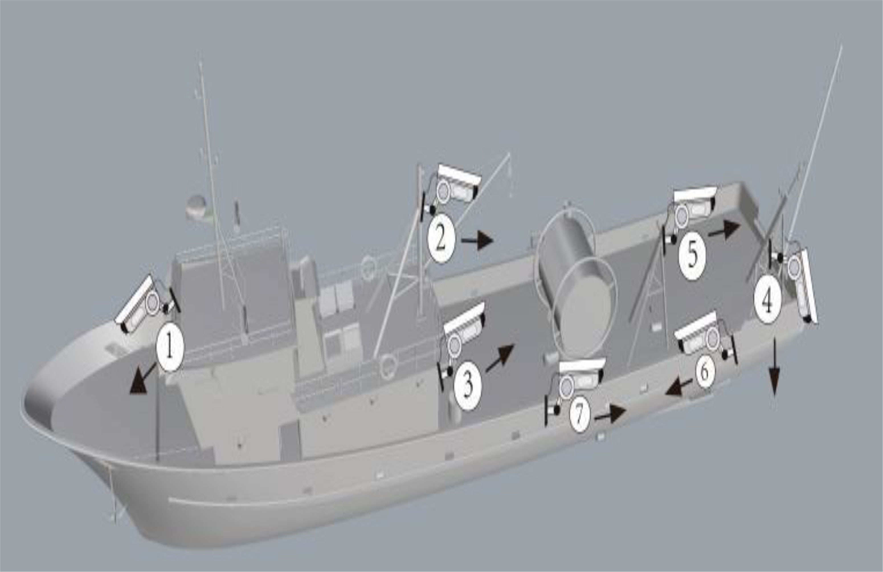
Figure 1 The position of the cameras in Xinhai vessels.

The present study aims to recognize the behavior of Chub mackerel fishing vessels, so only three sets of cameras numbered 2, 6, and 7 are mainly used. Camera 2 can be used to extract the winch behavior (pulling and putting nets) and the overall behavior of the vessels(sailing and waiting). Camera 6 was used to extract fish-related behaviors (“Waiting for fish”, “Fish in” and “Fish pick”). Camera 7 was also installed inside the cabin and had a particular overlapping area with camera 6, which can verify each other. In addition, camera 7 can also extract catch preparation behaviors, such as “Organize fish box”, “Reprint”, and the like. Therefore, nine behaviors such as “Sailing”, “Putting nets”, “Waiting”, “Pulling nets”, “Waiting for fish”, “Organize fish box”, “Fish in”, “Fish pick” and “reprint” can be extracted from the EMS data of Xinhai’s Chub mackerel fishing vessels. And the nine behaviors are reflected in the EMS data, as shown in Figure 2.

FIGURE 2

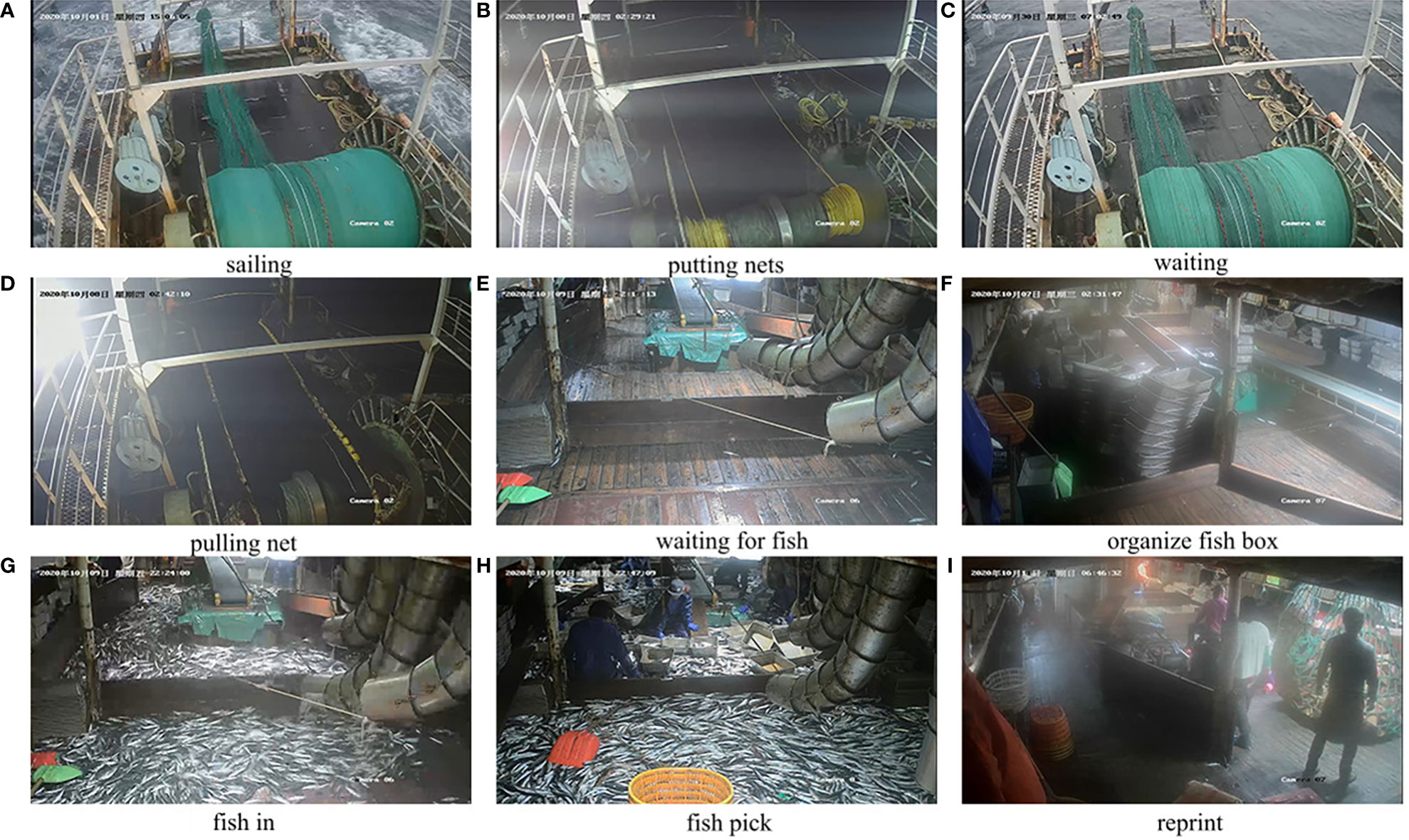
Figure 2 Nine kinds of ship behavior reflected in EMS.

Figure 2 shows that the above nine ship behaviors have their characteristics, but some of the behaviors have high similarities. Specifically, under the behavior of “sailing”, the lower end of the net is fixed on the hook, and the ship sails to find a suitable place for putting the nets. Under the behavior of “putting nets”, the winch rotates in the direction that the net is lowered into the sea. Under the behavior of “waiting”, there is no net (or only a tiny amount of net) wound on the winch. Under the behavior of “pulling nets”, the winch rotates in the direction of the net recovery. Under the behavior of “waiting for fish”, there is no catch in the fish entry room in the cabin. Under the “organize fish box” behavior, the crew stood in the fish entry room to organize the fish box and prepare to load the catch. Under the “fish in” behavior, the fish suction pump sucks the catch into the fish entry room. Under the “fish pick” behavior, the crew put the catch into the prepared fish box for processing. Under the behavior of “reprint”, the crew members put the loaded fish into the conveyor net, lift them out of the cabin and transport them to the transshipment vessel.

Among the nine vessel behaviors, “putting nets” and “pulling nets” have relatively high similarities, and it is difficult to distinguish them quickly with the naked eye. However, it is much easier for the naked eye to distinguish between these two vessel behaviors based on consecutive seconds of EMS video. To verify whether the neural network will encounter the same difficulty in extracting features of various vessel behaviors, we made two datasets of single-frame samples and multi-frame samples. The single-frame sample dataset is similar to that of most neural network classification tasks. Each sample included an EMS image as the data and a marked vessel behavior as the label. However, the dataset of multi-frame samples preserved specific temporal characteristics between EMS images. In the dataset of multi-frame samples, 100 consecutive EMS images were connected horizontally. The connected image was used as data, and each data was marked with a vessel behavior as the label. The structures of the above two datasets are shown in Figure 3.

FIGURE 3

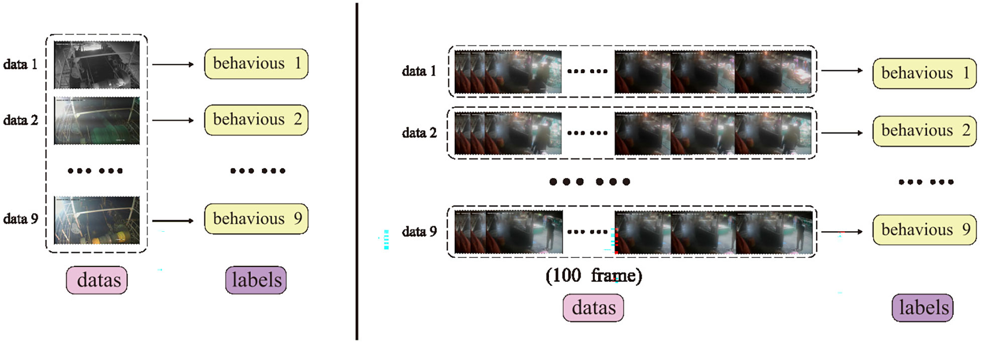
Figure 3 The structure of two types of datasets of single-frame samples and multi-frame samples.

No matter which data set is used, the size of the data set is exactly the same. Specifically, 23932 sets of data are divided into a training set (19146 sets of data), a validation set (2393 sets of data), and a test set (2393 sets of data) according to the ratio of 8:1:1. The training set is used to train the trainable parameters of the model, the validation set is used to adjust the hyper-parameters, and the test set is used to test the recognition effect of the models. These samples were obtained through the program and manual screening. First, write a script to extract 10s of images every five minutes from each video data. Subsequently, 23,932 data samples were manually screened out, including different sea areas and weather.

2.2 Pre-experimental method

The number of convolutional layers plays a crucial role in convolutional neural networks in general. However, some studies have shown that the number of convolutional layers is not strictly positively related to the effect of neural networks. An increase in the number of convolutional layers will inevitably lead to a significant increase in model sizes. Therefore, we first designed multiple convolutional neural networks with different numbers of convolutional layers purpose to roughly compare the effect of the number of convolutional layers on vessel behavior extraction and choose the most suitable one for extracting vessel behavior. In addition, the recognition of vessel behaviors may be applied to the real-time scene of EMS in the future. Real-time-related parameters such as model size and detection efficiency are essential reference factors for model selection. The present study designed four groups of parallel experiments with 3, 6, 9, and 12 convolutional layers, respectively. The convolution parameters of each convolutional layer had not been fine-tuned. The reason is that we want to roughly explore the impact of the number of convolutional layers on the recognition effect. The parameter values of each group of comparative experiments are shown in Table 1.

TABLE 1

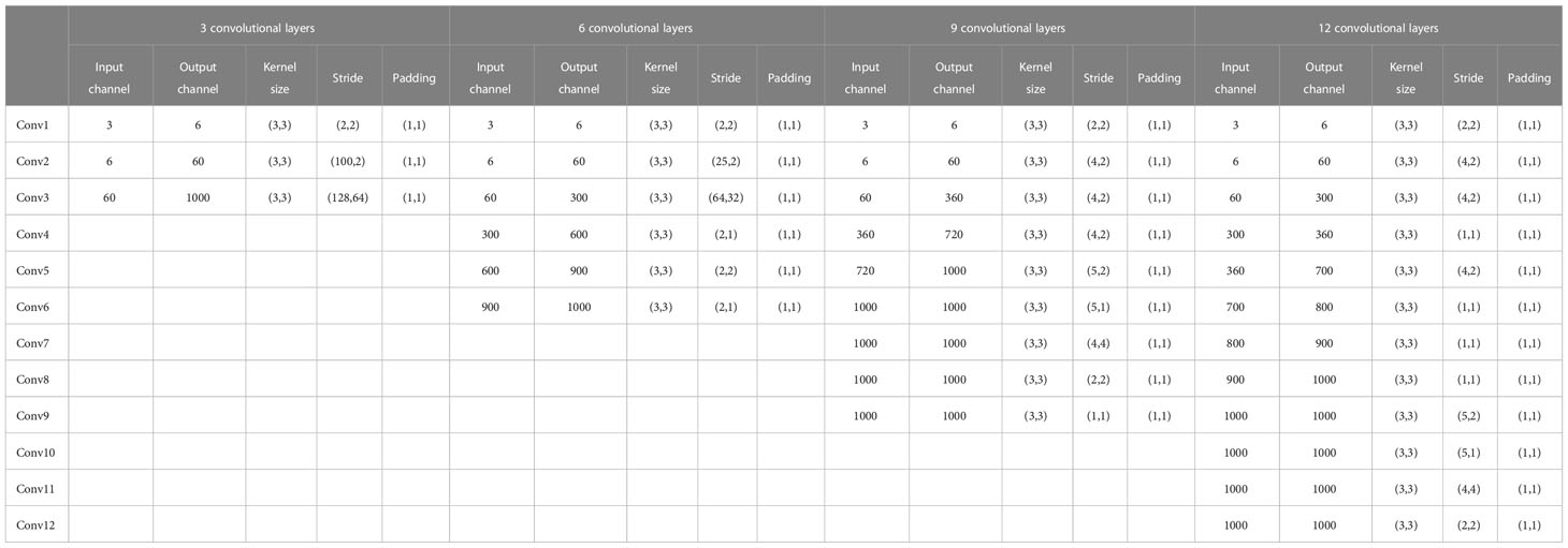
Table 1 Parameters of each group of the comparison experiments.

As mentioned in Section 2.1, apart from the network structure, the data set also significantly impacts the recognition performance. And two datasets in different formats had been created based on single-frame and multi-frame samples in the data processing stage. Therefore, we also need to compare the effects of the two different datasets on recognizing various fishing vessel behaviors in the pre-experimen.

2.3 Optimization methods

The various methods described in the pre-experiment section only roughly verified the feasibility of applying deep learning methods to recognize Chub mackerel fishing vessel behaviors and compared the number of convolutional layers and datasets on the recognition effect. The above procedures must be further improved if the behavioral recognition effect of Japanese mackerel fishing vessels is to reach an industrially usable level of operation. We designed multiple sets of experiments from the perspectives of the dataset and network structure to find out the most suitable method to be applied to the behavior recognition of Chub mackerel fishing vessels.

2.3.1 Data set optimization

The two designed datasets have their advantages and disadvantages. The dataset based on single-frame samples has a fast data loading speed and contains most of the data features. However, some fishing vessel behaviors have prominent characteristics of the time dimension. For example, the change of winches and nets at a particular time is the most apparent feature of the vessel behavior of “pulling nets”. But the dataset based on single-frame samples completely abandons these characters of the temporal dimension. The dataset based on multi-frame samples makes up for the defect of data loss in the time dimension of single-frame samples. Still, the sample size of 100 consecutive frames is too large, which may bring great difficulties to data loading and training and lead to some problems, such as long training time and low recognition efficiency. The FPS value of EMS video data is 25, which means that each multi-frame sample (100 data frames) includes 4 seconds of video data, so the data difference between two consecutive frames is minimal. Splicing 100 consecutive frames of data as a dataset sample is a waste of resources to a certain extent.

We proposed a new dataset creation method based on the above two datasets, which is a compromise method of the two datasets. Unlike the multi-frame sample dataset splicing 100 consecutive frames of consecutive images, the new dataset construction method skips the subsequent 19 frames after splicing one frame and splices the 20th frame of the image until each data sample contains five images. The construction method of the new dataset and the structure of the new data are shown in Figure 4. As shown in Figure 4, this new dataset sample is a subset of the multi-frame sample dataset, which preserves the most prominent temporal features of the samples in a skip-sampling manner. Compared with the multi-frame sample dataset, the new dataset discards the similar space features among similar frames but keeps the temporal features. It adds some of the most significant features in the temporal dimension relative to the single-frame sample dataset. Therefore, the data loading speed of the new dataset is better than that of the single-frame sample dataset in terms of feature extraction integrity due to the multi-frame sample dataset. The optimized 5-frame dataset still maintains the same size as the previously described dataset. And the comparison between different networks in the following is based on this optimized data set.

FIGURE 4

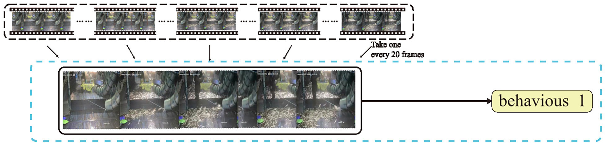
Figure 4 Datasets’ optimization method and optimized datasets’ structure.

2.3.2 Network structure optimization

The input vector of traditional artificial neural networks (ANN) such as multilayer perceptron (MLP) needs to be manually designed and calculated (Taud and Mas, 2018). However, previous studies have shown that feature vectors obtained by humans often cannot truly reflect the characteristics of the data, which is manifested in the fact that the classification application effect of artificial neural networks is lower than that of classifiers such as support vector machines. If the entire data of the whole image is used as a feature vector, it is a tremendous challenge for training the machine. And in the current situation, it is almost impossible and unnecessary. Therefore, Convolutional Neural Networks came into being. Since the advent of convolutional neural networks, the status of neural networks in image object detection and classification tasks has been dramatically improved. In recent years, neural networks have gradually become the preferred solution for image detection and object classification. In the fishery field, with a relatively low degree of informatization, neural networks have also been applied to a certain extent (Sarr et al., 2021; Selvaraj et al., 2022).

The convolutional layer is one of the most critical layers in the convolutional neural network. It consists of multiple convolutional units, and the back-propagation algorithm optimizes the parameters of each convolutional unit. Convolutional layers are used to extract features from input samples. Multiple convolutional layers are often used to extract different features in convolutional neural networks. For example, the first convolutional layer is used to extract image edge features, and deeper convolutional layers are used to extract color features. To further improve the comprehensive performance of convolutional neural networks, many scholars have made different improvements to the structure of neural networks. The more influential designs include pooling layers, long short-term memory modules, etc. In recent years, with the publication of the paper “Attention is all you need” (Vaswani et al., 2017), more and more scholars have chosen to use Transformer to achieve their various classification tasks. The attention mechanism has gradually been recognized. Therefore, in the current study, we mainly use the optimization method of adding a pooling layer, Long Short-Term Memory (LSTM) module, and attention mechanisms (including SE module and Convolutional Block Attention Module (CBAM)) to the convolutional neural network to compare the optimization effect of the network.

2.3.2.1 Pooling

The pooling method is actually a down-sampling method, and it was first seen in LeCun Y’s paper (LeCun et al., 1998), which the authors simply called “Subsample”. In 2012, AlexNet (Krizhevsky et al., 2012) was proposed, and this method was officially named “Pooling”. Standard pooling methods include max pooling, average pooling, random pooling, and combined pooling. The most common and currently used methods are max pooling and average pooling. The specific process of these two pooling methods is shown in Figure 5. The filters and stride parameters control the size of each pooling window and the jumping stride after each pooling.

FIGURE 5

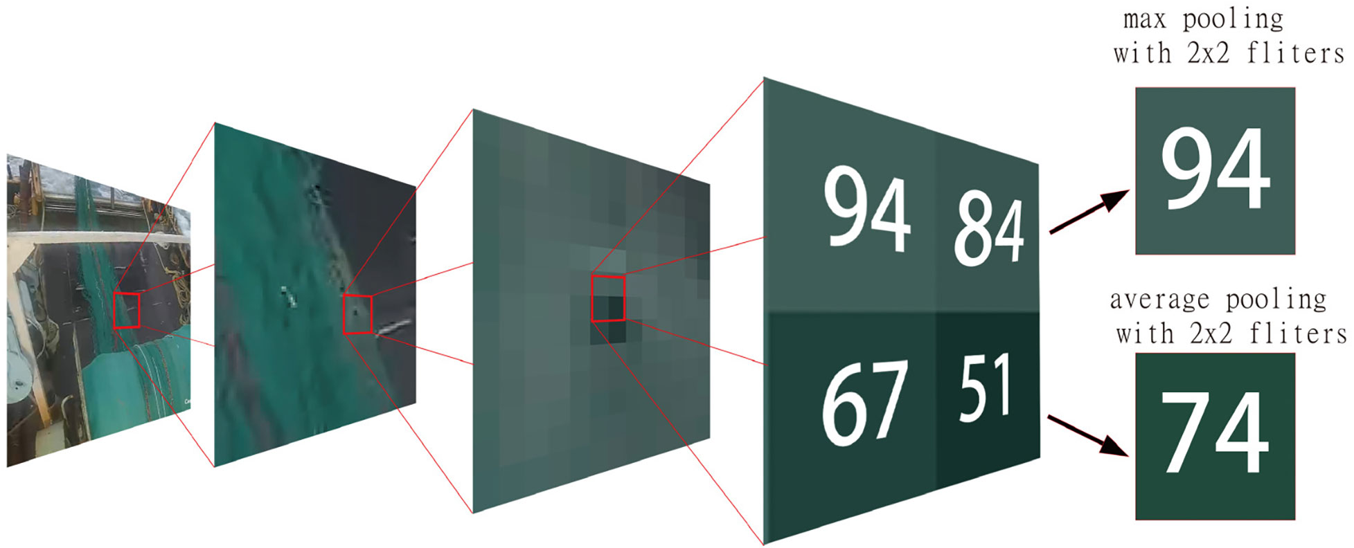
Figure 5 Demonstration of max pooling and average pooling.

In the current study, we try to reduce the magnitude of the network model by randomly adding max pooling and average pooling layers in the convolutional layers. Pooling layers are widely used to reduce model complexity while preserving as many data features as possible.

2.3.2.2 LSTM

Long short-term memory (Hochreiter and Schmidhuber, 1997) is a particular recurrent neural network (RNN), first proposed by Hochreiter and Schmidhuber in 1997, which can be used to learn time-dependent features. After the improvement and promotion of Alex Graves (Graves and Schmidhuber, 2005) and others, LSTM has been widely used in many fields now. Traditional recurrent neural networks pass forward with a single state, and gradient explosion or disappearance problems are prone to occur during long-sequence training. Compared with the traditional recurrent neural network, the most significant feature of LSTM is that it adds a new transfer state, that is, the cell state. The structure of a classic LSTM is shown in Figure 6. LSTM mainly includes three processing units: Forget Gate, Input Gate, and Output Gate. The forget gate is primarily responsible for the selective forgetting of the pre-node cell state. The input gate is responsible for selective memory of the current node input. The output gate is responsible for determining the output of the current node.

FIGURE 6

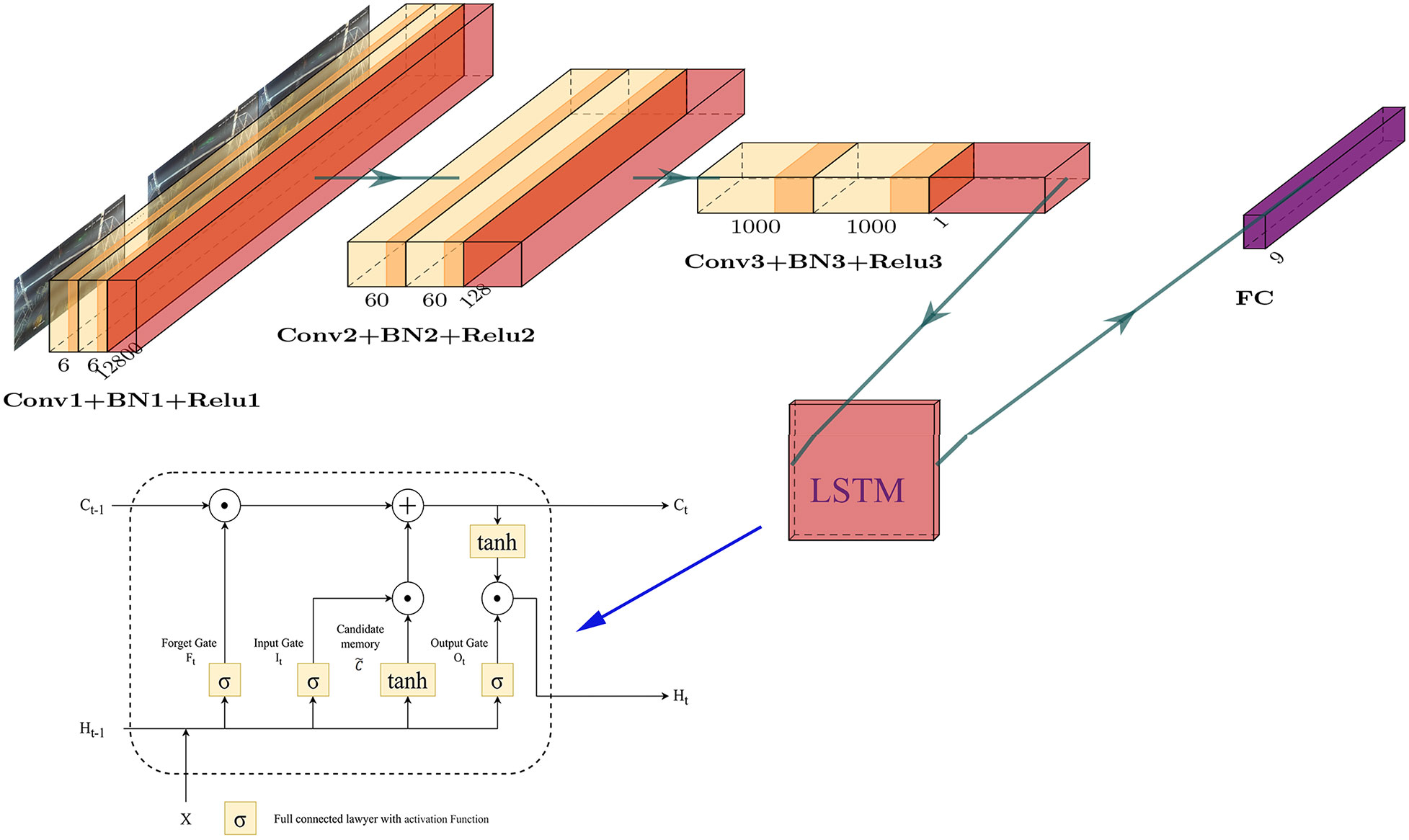
Figure 6 The structure of the LSTM module and the position of the LSTM module in the network.

Both the 100-frame sample data set in the pre-experiment and the optimized 5-frame sample data set have long-sequence features to a certain extent. Therefore, adding an LSTM to a convolutional network might be able to enhance the feature extraction capability of the network, especially for the temporal dimension.

2.3.2.3 Attention mechanism

In a traditional convolution operation, all channels and regions of each channel have the same weight, which is significantly different from how humans observe things. The attention mechanism aims to distribute the weights of the input more reasonably. The attention mechanism and pooling have certain similarities from an algorithmic point of view, and it can even be said that pooling is a unique (average-weighted) attention mechanism. Or the attention mechanism is a generalized pooling that redistributes the input weights. Attention models such as SE and CBAM are commonly used in the current convolutional neural networks.

SENet won the classification task of the 2017 ImageNet competition. Compared with the previous convolutional neural networks, its most significant feature and contribution are the proposed Squeeze-and-Excitation (SE) module. The SE module expects the machine to learn the importance of different channels automatically. As the name suggests, the SE module is mainly composed of two essential operations, Squeeze and Excitation. What Squeeze does is a global average pooling operation. The attention mechanism hopes to obtain the feature relationship between channels. Still, the convolution operation is always performed in a specific part, and it is difficult for any convolution layer to receive the complete information in a channel. This feature is more evident in the convolutional layers located at the front. The receptive field of the convolutional layer at the front of the network is relatively small, reflecting a small proportion of information in a channel. Therefore, the Squeeze operation in SE encodes the spatial features on the entire channel as a global feature. This encoding process is implemented by global average pooling, as shown in Equation 1.

$\begin{array}{ll}{z}_{\text{c}}=F_{\text{sq}}(u_c)=\frac{1}{H\times W}{\displaystyle \sum _{i=1}^H{\displaystyle \sum _{j=1}^W{u}_c(i,j)}},z\in R^C& (1)\end{array}$

In Formula 1, F_sq(u_c) represents the Squeeze operation performed by SENet on the input matrix u_c, and z_c is the output of this operation. H and W represent the height and weight of u_c, respectively. u_c(i, j) represents the value of the input matrix u_c at row i, column j. z_c has all the receptive fields in the channel with the squeeze operation. After getting the description of the global features of an entire channel, the attention mechanism also needs to find the relationship between each channel. The relationship between the individual channels is non-linear and cannot be one-hot. Therefore, the Excitation operation in the SE module uses the gating mechanism of sigmoid functions to capture the relationship between channels. And this gating mechanism is shown in Equation 2.

$\begin{array}{ll}s=F_{\text{ex}}(z,W)=\sigma (g(z,W))=\sigma (W_2\mathrm{Re}\text{LU}(W_1,z))& (2)\end{array}$

In Formula 2, F_ex(z, W) represents the Excitation operation performed by SENet, z is the input of the operation, and s is the output of the operation. ReLU represents the activation function of ReLU and σ represents the activation function of sigmoid. W₁ and W₂ are two fully connected layers, which are used to train the weight values of different channels. After learning the sigmoid activation values for each channel, multiply the activation values by the original feature values. The structure of SENet is shown in Figure 7. Therefore, the purpose of the entire SE module is to learn the weight of each channel so that the model can learn more pertinently for each channel. To prove the potent portability of the SE module, SENet also did experiments to embed SE module into classical ResNet and VGG and achieved a lower error rate (top-5 err) and parameter amount (GFLOPs).

FIGURE 7

Figure 7 The structure of SENet.

Convolution Block Attention Module (CBAM) is an attention module proposed by S Woo et al (Woo et al., 2018). in 2018. CBAM includes two necessary sub-modules, Channel Attention Module (CAM) and Spatial Attention Module (SAM), whose structure is shown in Figure 8. Channel Attention Module is a channel-based attention mechanism, and its design idea is very similar to the SE module. The most apparent difference between CAM and SE in structure is that CAM adopts the parallel method of max pooling and average pooling to extract channel features. The processing process of CAM after two parallel pooling is the same as SE, which is to reduce the dimension first and then increase the dimension. The difference is that CAM adds the operation results of the two parallel pooling layers before performing sigmoid activation and multiplying it with the original feature map. Woo’s experiments show that parallel pooling layers perform better than a single global average pooling. In addition to focusing on the weights on individual channels, CBAM also uses SAM to assign different weights to spatially other regions. The operation of SAM is after CAM (experiments have shown that this order can get better results). SAM uses the feature map obtained by the CAM module as the input value and then performs two pooling whose size of the pooling window is the number of column channels. The feature map obtained by the first pooling is convolved with the feature map obtained by the second pooling, the purpose is to compress the channel, and finally, sigmoid is performed. This spatial attention mechanism makes the machine pay more attention to the regions with more target information in the image, which is closer to the process of human learning tasks. To prove the portability of the CBAM module, Woo, like the authors of SENet, embedded the CBAM module in classic networks such as ResNet and MobileNet. The performance gains on these networks demonstrate the effectiveness of CBAM. In addition, the visualization results of the weight data on regions and channels show that the network which has added the CBAM module pays more attention to the areas with richer target information. This visualization method also improves the interpretability of the CBAM module.

FIGURE 8

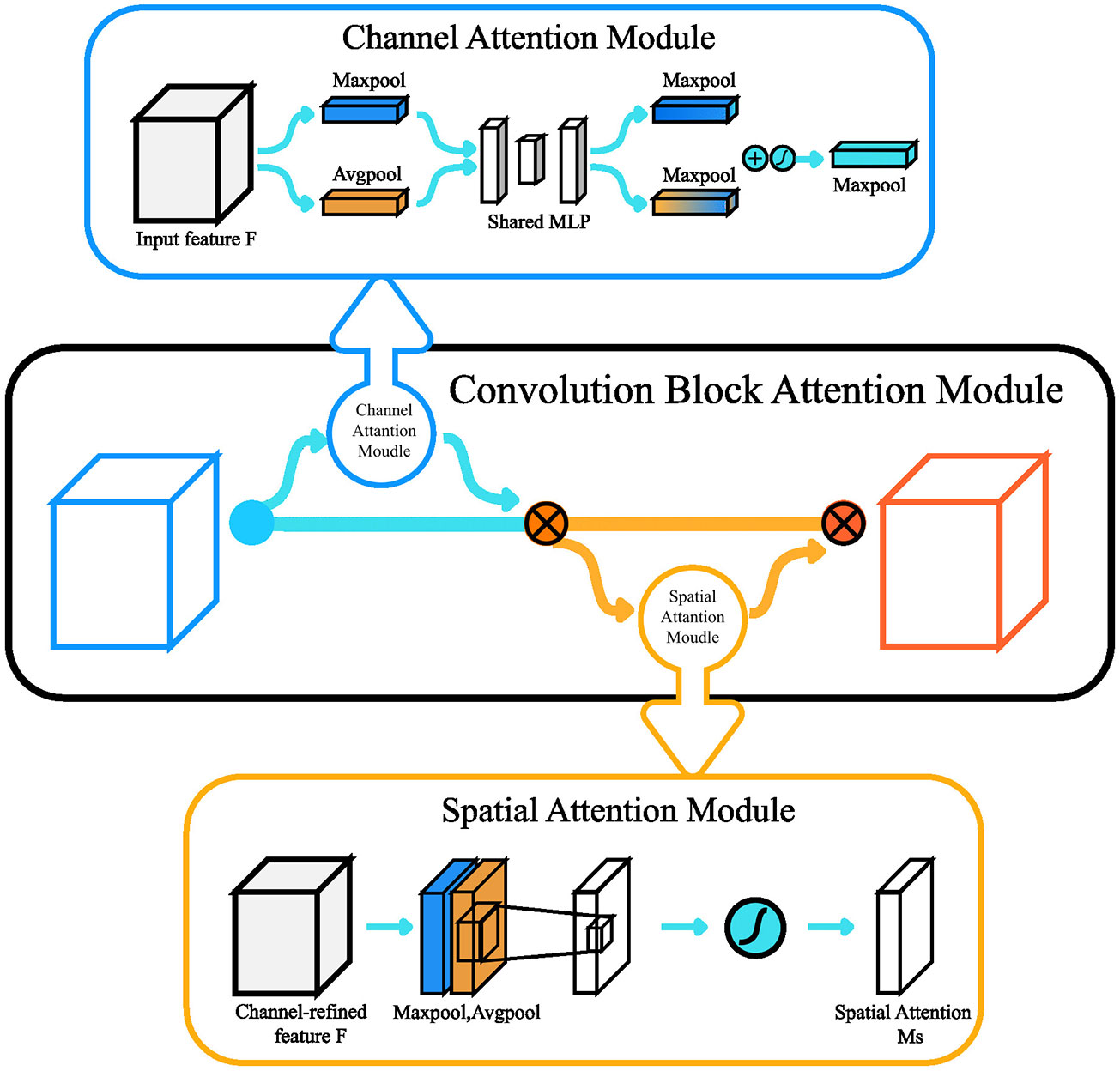
Figure 8 The structure of the CBAM module.

In the current study, four groups of experiments were designed in combination with the above various network optimization methods to compare the effects of different combinations of these optimization methods on the network performance. The optimization methods used in each group of experiments are shown in Table 2.

TABLE 2

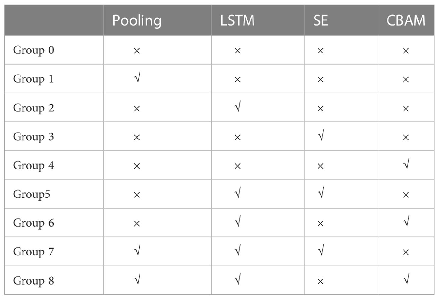
Table 2 Experimental group information for network structure optimization.

Described below are the locations of the various modules in the network. The pooling layers used in the experiments appeared after each convolutional layer and alternated between max pooling and average pooling. Attention modules such as SE and CBAM were designed in the convolutional layer at the front of the network and the network’s last layer to extract the attention under different receptive fields. The attention mechanism may play a greater role in the front and back positions in the network. And in our several sets of experiments, when the attention module is placed after Conv2, the performance of the network is better than that after Conv1. The LSTM module is designed after the last convolutional layer. If there was an attention module after the final convolutional layer, the LSTM was created after the attention module. Each network with the LSTM optimization module includes only one LSTM module. The length of the time step of each LSTM module is 5, and the number of hidden layers of is 20. There are two reasons for setting the time step value to 5. The first reason is that after multiple comparison experiments, the model can exert the greatest performance effect when the time step is 5. The second reason is that we believe that the behavior of fishing vessels may have a certain correlation with the five consecutive samples before and after. Taking a 9-layer convolutional network as an example, Figure 7 shows the location of each module in the network. It should be noted that the convolutional layers (Conv1, Conv2, etc.) in Figure 9 actually contain a Convolution layer, a Batch Normalization layer (Santurkar et al., 2018), and a Rectified Linear Unit (Xu et al., 2015). Since such combinations are common collocations in neural network design, they are simply called “Conv x” in Figure 7.

FIGURE 9

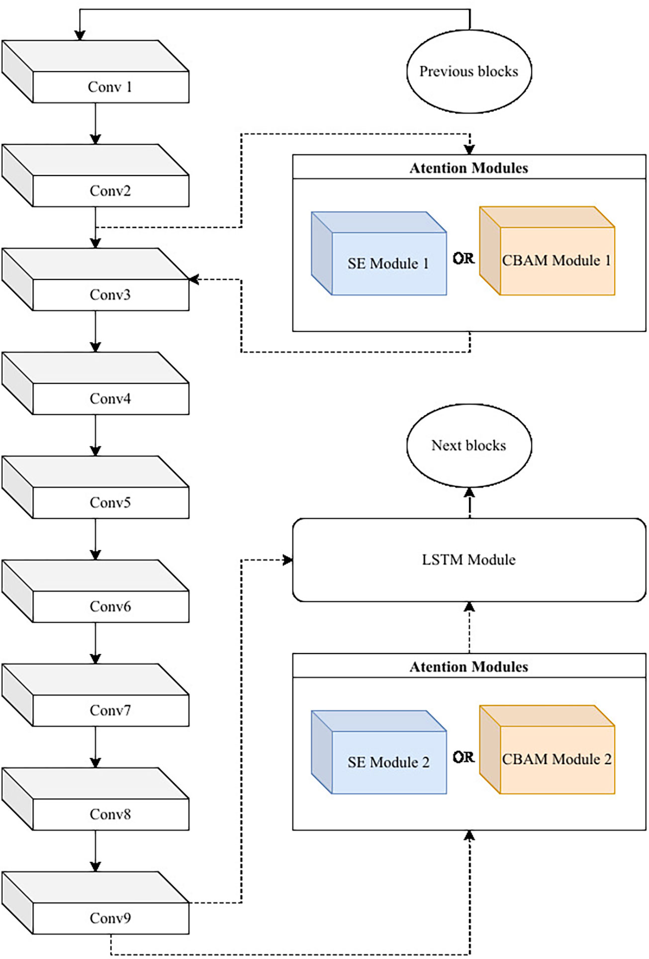
Figure 9 The position of each optimization module in the 9-layer convolutional network.

3 Result

3.1 Results of the pre-experiment

In the pre-experiment, 3-layer, 6-layer, 9-layer, and 12-layer convolutional networks were designed to find out the relationship between the number of convolutional layers and the effect of ship behavior recognition, which purpose is to choose the most suitable number of layers for the subsequent formal experiments. The F1 score (Goutte and Gaussier, 2005) is used to represent the recognition effect of the network model. This is because the F1 score is a comprehensive reflection of the Precision and Recall parameters, which can better represent the actual effect of the model. It is also one of the most common evaluation indicators in deep learning tasks. The Loss value reflects the classification loss value of the model. This research selects the classic cross-entropy loss (Zhang and Sabuncu, 2018) as the criterion for judging the classification loss. Low Loss, high Precision, high Recall, and high F1 score mean better model classification results. This research is typical applied research. In addition to the requirement of high accuracy, the ship behavior recognition model should also pursue lightweight and high efficiency as much as possible. Therefore, when judging the most suitable network model for ship behavior recognition, the network training time and the size of the network model are also considered. Figure 10 shows the performance of four different network models on classification parameters (a), model size (b), and training time (c). The above classification parameters refer to the performance of each model in the test set.

FIGURE 10

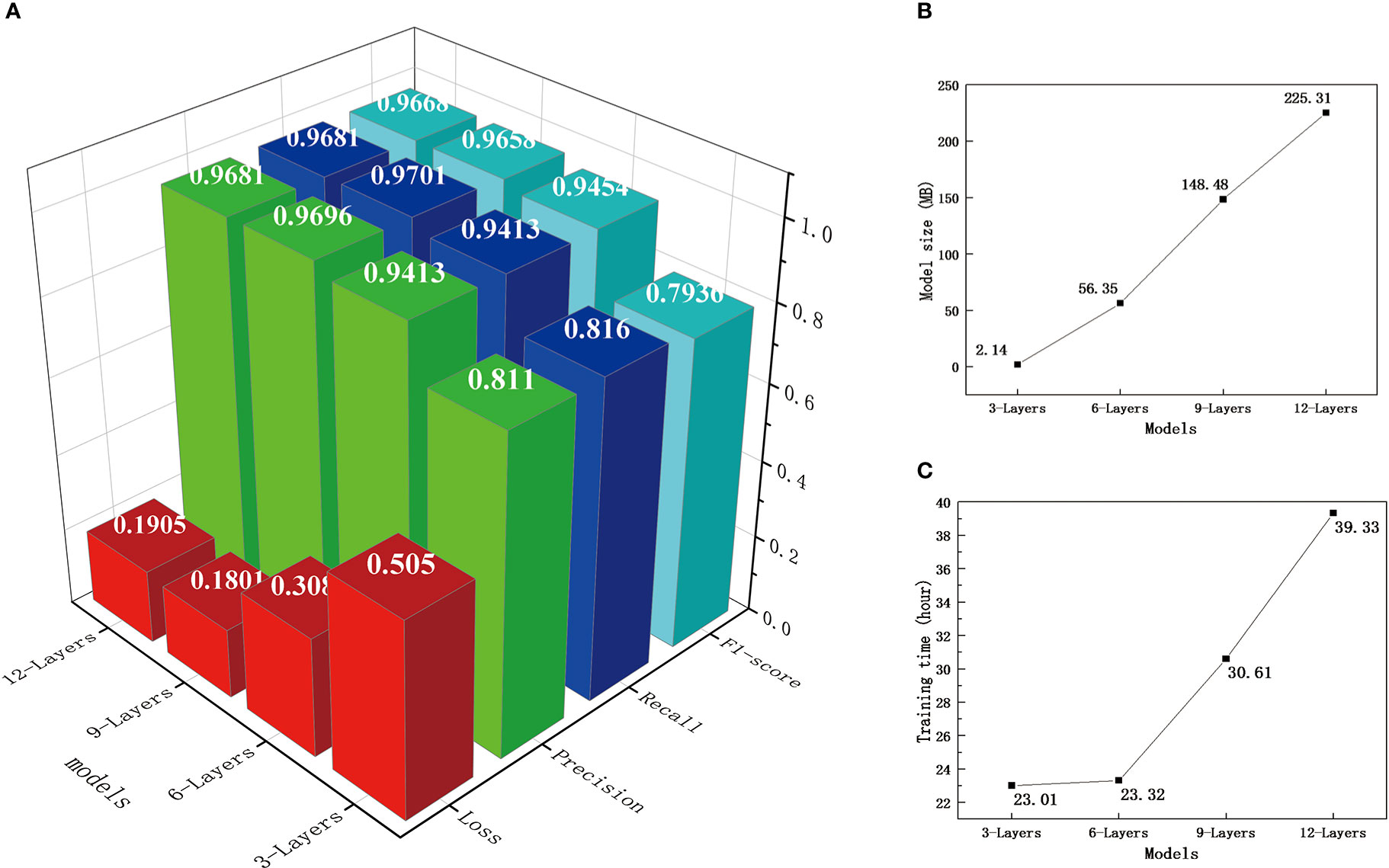
Figure 10 Comprehensive performance of network models with different convolutional layers. Part A is the effect comparison of models with different convolutional layers, Part B is their Size comparison, and Part C is their training time-consuming comparison.

Figure 10 shows that the number of convolutional layers has a significant impact on the classification performance of the neural network, the size of the neural network model, and the training time. Within a specific range, the increase of the number of convolutional layers can significantly improve the classification effect of the model. However, once the improvement effect of this method is saturated, the classification effect cannot continue to improve with the increase in the number of convolutional layers. It might even go backward (from a 9-layer convolutional to a 12-layer convolutional network). With the increase in the number of convolutional layers, the model’s size and the training time increase significantly. The increase in the number of convolutional layers leads to a rise in the number of parameters, inevitably leading to an increase in model size and training time. Therefore, this research selects the 9-layer convolutional neural network with the best classification effect and all-around performance as the primary condition in the formal experiment.

In addition to studying the impact of the number of convolutional layers on the network’s overall performance, the pre-experiment also compared the effect of two different datasets, the single-frame sample dataset and the multi-frame sample dataset. The single-frame sample and multi-frame sample data sets were trained for 100 Epochs under the 9-layer convolutional network, which took 1.98 hours and 30.61 hours, respectively. Therefore, the single-frame sample data set can significantly shorten the training time compared to the multi-frame sample data set. Experimenters infer a single frame of sample data before the experiment and may confuse the two ship behaviors of “Putting Nets” and “Pulling Nets”. To test this conjecture, Figure 11 shows the ability of the model to distinguish ship behavior under the two datasets using a confusion matrix.

FIGURE 11

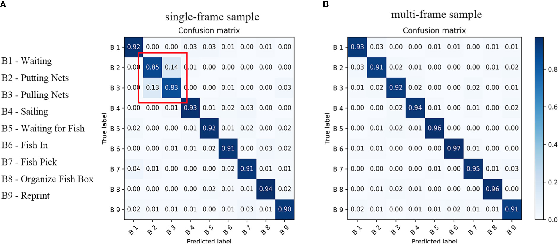
Figure 11 Confusion matrix for two different datasets in test set. Part A is the confusion matrix of a single-frame dataset, and part B is the confusion matrix of a multi-frame dataset.

Figure 11 shows that the comprehensive performance of single-frame data samples is significantly worse than that of multi-frame data samples, especially the ability to distinguish between the two behaviors of “Putting Nets” and “Pulling Nets”. However, the multi-frame sample data sets training takes too long, and the practical application is complex. The above comparison data shows that increasing the number of frames of data samples can improve the network’s ability to extract features. Still, it will also have a relatively significant negative impact on the training time. Therefore, it is necessary to design a compromise between the two datasets to ensure that the network can extract enough features while reducing the training time as much as possible.

3.2 Results of optimization

The 9-layer convolutional neural network takes 2.72 hours to train for 100 epochs in the optimized 5-frame sample dataset, which is much lower than 30.61 hours in the 100-frame sample dataset. And the F1 score of this model in the test set reached 0.9665, which is close to the F1 score (0.9797) of 100-frame samples. Therefore, the optimized dataset is more suitable for application in the vessel behaviors recognition task in the current study.

The addition of the pooling layer, SE, CBAM, LSTM, and other modules (and their different combinations) impacts the network model’s training process and recognition effect. During the training process of 100 epochs, the change process of F1 score in each group of models in the training set is shown in Figure 12. The impact of adding these optimization modules on the F1 score of the models in the training set is mainly reflected in the first 20 Epochs. The reason is that, after enough epochs, each parameter gradually reaches a convergent state, and the F1 score will oscillate slightly around the saturation state. As a result, the second half of Figure 12A has a cluttered crossover (although some data points have been removed from the second half). Therefore, Figure 12B illustrates the enlarged data for the first 20 Epochs to clearly show the optimization module’s impact on the training process.

FIGURE 12

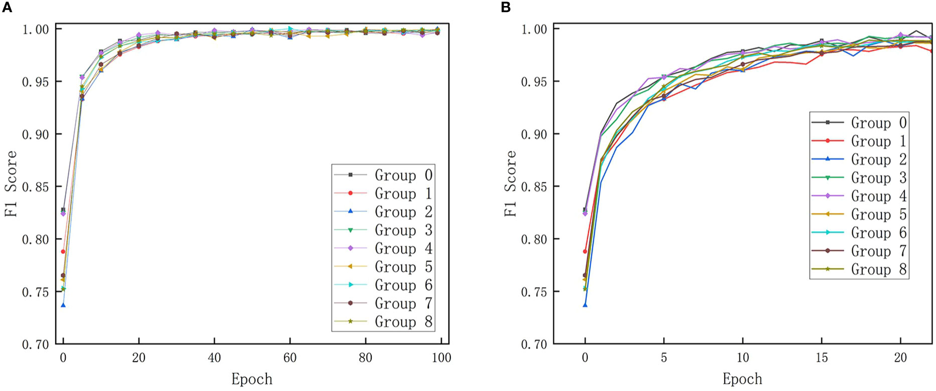
Figure 12 Changes in F1 score during training. Part A is the parameter change of 100 epochs, and part B is the parameter change of the first 20 epochs.

Figure 12 shows that, compared with the control group (Group 0), the addition of each optimization module does not significantly accelerate the convergence process. Only the CBAM module showed a small effect of accelerating the convergence, and the convergence speed of the other groups was even slightly lower than that of Group 0. However, the convergence process is not an important factor in selecting network models in the current study. Although the convergence rates of these experimental groups were inconsistent, the gap between them was small. In practical applications, factors such as recognition rate and model size will have a more direct impact on economic benefits. In order to verify whether the addition of different optimization modules will have a significant impact on the detection accuracy of the model. We performed Single-factor analysis of variance with different groups as the independent variable and the detection accuracy as the dependent variable. The results of the analysis are shown in Table 3.

TABLE 3

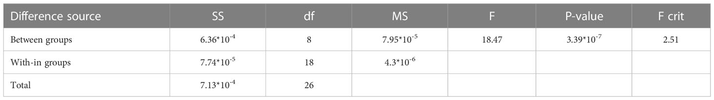
Table 3 The result of Single-factor analysis of variance with different groups.

Table 3 shows that the P-value between groups is 3.39*10^-7, which is far less than 0.01, and the F value between groups is 18.47, which is greater than F crit(2.51). Therefore, the selection of different optimization modules has a very significant impact on the recognition effect of the model. Below I will show the specific performance of each group in the ablation test in Table 4, purpose to more clearly show the differences between the groups. The training time, model size, and parameter performance of the model in the test set of each experimental group are shown in Table 4. And the P, R, F1, and L in the Indicators directory in Table 4 represent Precision, Recall, F1 score, and cross-entropy loss, respectively. Params represents the parameter quantity of the model, and FLOPs(floating point operations) is used to measure the calculation amount of the model.

TABLE 4

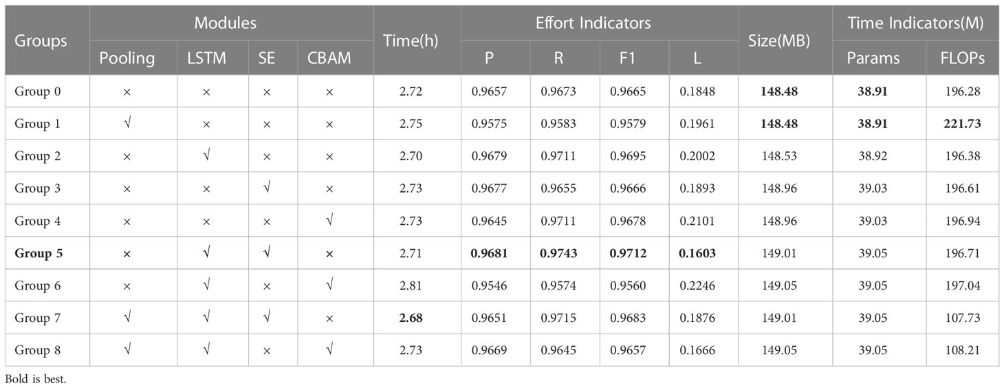
Table 4 Comparison of test results of each group.

Table 4 systematically presents the results of each group of experiments. In terms of training time, the addition of the single optimization module increased training time except for the LSTM module, but the increase is slight (between 0.3% and 3%). The LSTM module is a particular case. The addition of the LSTM module shortens the training time of the basic 9-layer convolutional network (Group 0) and the 9-layer convolutional network with the SE module (Group 3). Still, it increases that of the 9-layer convolutional network with CBAM (Group4). However, whether this situation is an inevitable phenomenon caused by the modules or an accidental phenomenon caused by the load of the training machine remains to be further verified. In terms of the model size, the addition of each optimization module increased the model size. Compared with the number of convolutional layers, the addition of the optimization module has little impact on the model size. In terms of the recognition effect of the test set, the addition of LSTM, SE, and CBAM modules all have a positive impact on the F1 score indicator in the test set. The impact of the pooling layer on the model is more complicated. When the pooling layer is added to the network without any optimization module, the recognition effect of the model becomes worse, and the number of parameters and FLOPs are not significantly reduced. However, when the pooling layer is added to the network with the attention mechanism, the FLOPs of the model are significantly reduced, and the drop even reaches about 45%. The optimization effect of the pooling layer on the CBAM attention mechanism is particularly obvious, and the recognition effect is improved a little under the premise of greatly reducing FLOPs.The combination of LSTM and SE performed best in each group of experiments, and the combination of LSTM and CBAM performed the worst in each group of experiments. Before adding LSTM, SE was very close to CBAM. To further observe the optimization effect of SE and CBAM modules on the network, the network’s weights in Group 3 and Group 4 before entering the LSTM module are recorded and restored in the receptive field in the form of heat. As shown in Figure 13, SE and CBAM have significant differences in the attentional points. Taking the “Waiting” behavior in the figure as an example, the attention of SE and CBAM modules are obviously focused on the reeling machine and the nearby sea, but there are some differences in the specific distribution of their attention. SE’s attention is focused on the position of the reeling machine in the last three frames. In comparison, CBAM’s attention is focused on the middle part of the first three frames. This distribution of attention also has a logical explanation. Behaviors captured by the same camera have a relatively high similarity. The “waiting” behavior is captured by the camera 2. In addition to the “waiting” behavior, the camera 2 also captures three behaviors of “pulling net”, “putting net” and “sailing”. Compared with the behaviors of “pulling net” and “putting net”, the “waiting” behavior has the biggest difference in that the reeling machine under the “waiting” behavior will not rotate. Compared with the behavior of “sailing”, the main characteristic of the behavior of “waiting” is that its sea surface has no waves. Both SE and CBAM focus on the two key areas of the reeling machine and the sea surface, but they are distributed on the left and right sides of the sample. This is also one of the explanations for the poor performance of CBAM with the LSTM module and the better performance of SE with the LSTM module. The attention mechanism mainly optimizes the classification effect of images by adjusting the weights in different spaces and channels. SE and CBAM showed a large effect difference in this experiment. Judging from the effect in Figure 13, there are indeed some differences in the focus areas of the two attention mechanisms. From a structural point of view, in addition to adding a spatial attention mechanism, the biggest difference between CBAM and SE is that CBAM uses both maximum pooling and average pooling, while SE only uses average pooling. The choice of pooling method is also likely to be the reason why SE is significantly better than CBAM in the experiments in this paper. In short, The SE attention mechanism mainly adds the weight of the space, while the CBAM adds the weight of the channel on the basis of SE. This structural difference leads to different weights of the two attention mechanisms on different receptive fields. However, we still don’t have a firm conclusion as to why this different weighting leads to a large difference in the model results. The above analysis is only the author’s speculation from the structure and receptive field, and the verification of this speculation still needs to be followed up by follow-up research. How the attention mechanism affects the classification performance of the model is still an important issue worthy of research.

FIGURE 13

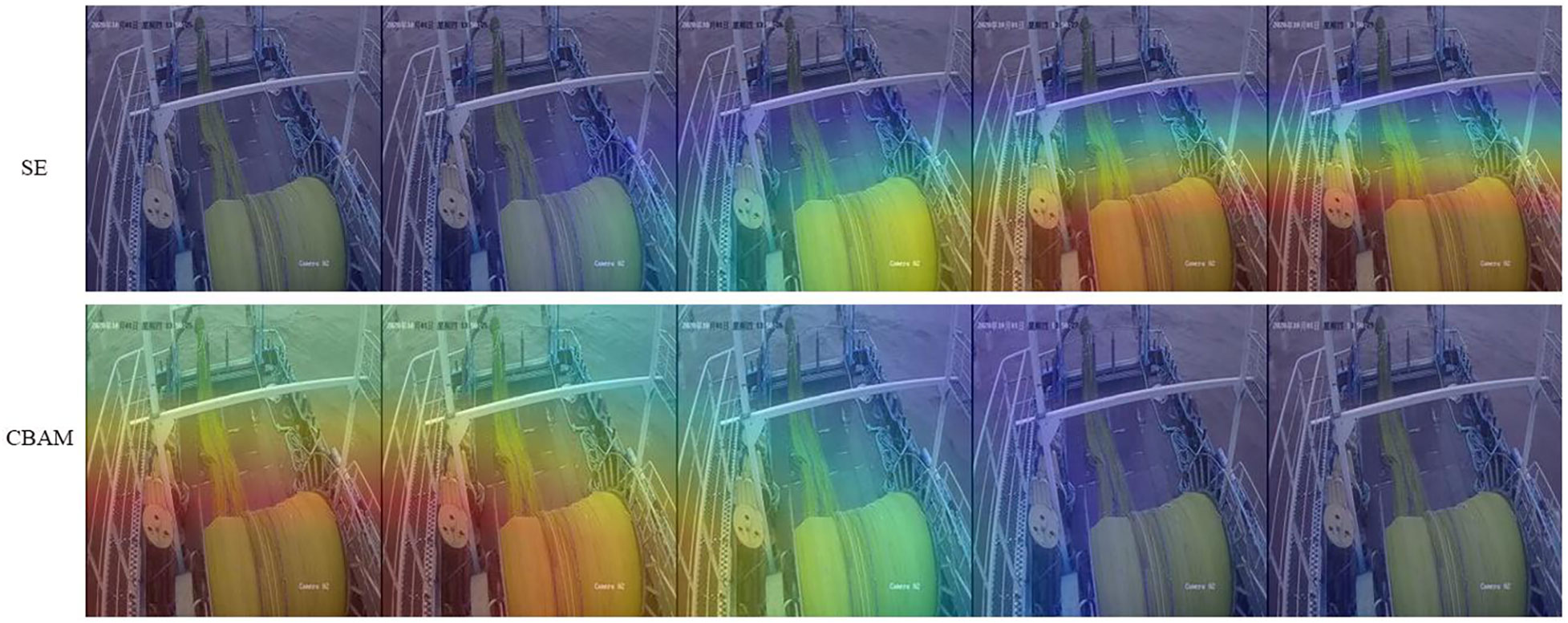
Figure 13 Attention of SE and CBAM.

This research can be considered as a special image classification problem technically. In the field of image classification, there are already excellent classic models such as AlexNet, VGGNet, and ResNet. In the dataset of behavior recognition of Japanese mackerel fishing boats, the model we designed is more targeted and achieves better recognition results. The comparison data between the classical model and our model are shown in Table 5.

TABLE 5

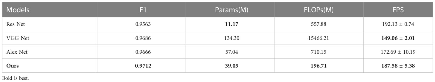
Table 5 Comparison of accuracy and efficiency of the models.

In Table 5, Ours refers to the Group 5 with the best performance in the ablation test. Table 5 shows that among Res Net, VGG Net, Alex Net, and our model, our model performs best in F1 score, Params, and FLOPs. The FPS (Frames per second) in the table is the average detection efficiency of 10 detections on the test set. Although the FPS value of our model detection efficiency is slightly lower than that of ResNet, the detection efficiency of 187.58 has exceeded the FPS of the video (25), so the detection efficiency of our model can meet the real-time requirements.

4 Discuss

This research mainly studied the feasibility of applying a convolutional neural network in the behavior recognition of Chub mackerel fishing vessels by using the data of the vessel’s electronic monitoring system. The number of convolutional layers, pooling layers, LSTM module, SE module, CBAM module, and other factors (and different combinations of each factor) are compared to the recognition effect of vessel behaviors and the impact of the model’s size. The experimental results showed that the number of convolutional layers could significantly impact the recognition effect and the magnitude of the network. With the increase in the number of convolutional layers, the volume of the network also increases significantly, and within a specific range, the recognition effect is also considerably improved. However, the improvement of the recognition effect is not linear. After the recognition effect is saturated, the increase of the number of convolutional layers can no longer improve the recognition effect and may even reduce the recognition effect. The purpose of adding the pooling layer is to reduce the magnitude of the network. After adding the pooling layer, the size of the network model is indeed significantly reduced. Still, the addition of a single pooling layer has a negative impact on the recognition effect in a certain extent. It is for this reason that pooling layers have been used less and less in mainstream neural networks in recent years (Springenberg et al., 2014). In data sets with time-series features (100-frame sample data set and optimized 5-frame sample data set), the LSTM module has a relatively pronounced improvement effect. Moreover, the addition of the LSTM module will only increase the size of the network model by a small margin. Relative to this slight increase, the positive impact of the LSTM module on the recognition performance is quite apparent. SE module and CBAM module are two of the most widespread attention mechanism modules due to their powerful optimization effect and portability. The addition of these two modules had a particularly positive impact on the recognition effect.

The current study further proved the feasibility of applying electronic monitoring data to recognize vessel behaviors and specifically proposed a deep learning-based vessel behaviors recognition scheme. Before the promotion of electronic monitoring, ship behavior often needed to be recorded manually or extracted based on ship position data. But both methods have apparent flaws. The manual recording method requires higher labor costs, and the recorded data is highly subjective. In addition, due to the impact of COVID-19, new challenges have arisen in the dispatch of professional human observers (Sorensen et al., 2020). Vessel behavior recognition methods based on vessel position data have more substantial objectivity, and vessel position data are generally obtained through AIS or VMS. The main problems of vessel behavior recognition methods based on position data were the limited number of identifiable behaviors, the low recognition success rate, and the difficulty of verification. For example, when the VMS data showed that the speed of the fishing vessel was 0, it is difficult for the vessel behavior identification methods based on the vessel position data to determine whether the vessel is in the “Stop” behavior or the “Pulling Net” behavior. The vessel behaviors recognition methods based on electronic monitoring can avoid the above problems well. The electronic monitoring system records the most real visible data in vessels. The amount of information contained and the objectivity of the information is much higher than those of the other two schemes. Because of the enormous amount of information in video surveillance data, we can identify various vessel behaviors of research value from the data of electronic monitoring systems. Table 6 compared the characteristics of the above three types of vessel behaviors recognition methods.

TABLE 6

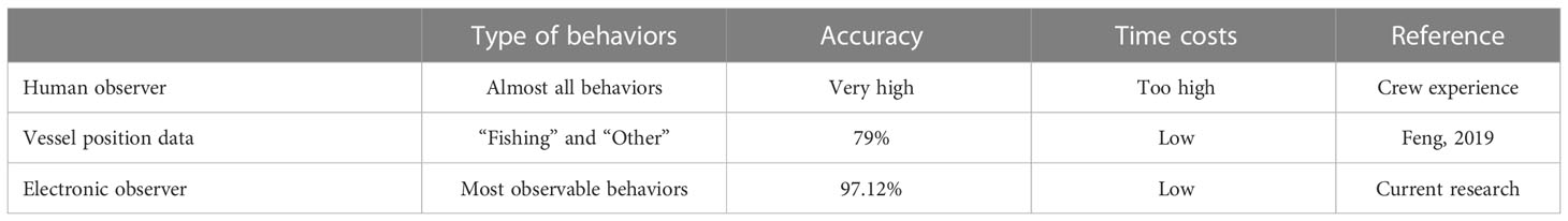
Table 6 Comparison of three methods of ship behavior recognition.

The vessel behaviors recognition method proposed by this research had strong feasibility. However, due to the influence of various factors such as time, there is still some room for improvement. After it had been determined in the pre-experiment that nine convolutional layers are more suitable for the behavior recognition of this dataset, the subsequent network model optimization was carried out in the 9-layer convolutional network. This experimental scheme defaults to the premise that the addition of LSTM, SE, CBAM, and other modules will not change the influence of the number of convolutional layers on the recognition rate of the network model. Still, this premise has not been fully proved. Although the increase in the number of convolutional layers will significantly improve the recognition rate, it will also considerably increase the model size. Suppose a lighter network such as 6-layer and 3-layer is optimized, and its optimization effect can exceed that of a 9-layer convolutional neural network. In that case, it will have greater economic significance (a lightweight network means lower computational cost). Since Group 0 of the control group has achieved a good recognition effect, the optimization space for Group 0 of Group 1-8 is relatively limited. In the construction of the data set, the data samples of 5 frames may not be the best construction method. However, there are many optional frames for data set construction, and it is difficult to compare all possibilities through an exhaustive method. In addition, the 5-frame data set has been able to meet the industrial requirements in terms of detection effect and detection efficiency. Adjusting the optimal data set frame number may be one of the directions for further optimization in the future. Although this paper compares the designed model with the classic Res Net, VGG Net and Alex Net, the comparative research is still insufficient. For example, convLSTM is a common combination of convolutional neural network and LSTM. Follow-up research can continue to compare the model of this paper with the models with convLSTM architecture. In addition, the use of electronic monitoring data in this study is still insufficient, and there may be more than the nine types of ship behaviors that can be mined with research value. In addition, the structures of the fishing vessels participating in the experiment are similar, and the universality of the network model has not been fully verified yet. The best model proposed in this paper may only perform best in a specific fishing boat, and the generality of the model should be further improved in the future. Expanding the use of models has important implications for fisheries, but requires data and industry support. There is still a long way to go for a highly versatile fishing boat behavior recognition model.

Electronic monitoring systems, known as “electronic observers”, are considered the next generation ship management system with the most potential to replace human observers due to their significant advantages in data recording (Evans and Molony, 2021). However, the current ship’s electronic monitoring system is still in its infancy. And there are still many problems, such as the lack of efficient and feasible methods for the processing of electronic monitoring system data. The vessel behaviors recognition method proposed in this study is of great significance to the data processing of electronic monitoring systems. The future electronic monitoring system is bound to rely less and less on humans, so in addition to the automation of the data acquisition part, the data processing part also needs a higher degree of automation. It is of great significance to study the application of electronic monitoring systems in vessel behavior recognition for building a complete intelligent electronic monitoring system. The current electronic monitoring system has the problem that the data capacity is too large. An electronic monitoring system needs to be equipped with a hard disk of dozens of TB, and the storage and transmission costs are too high. Therefore, we will focus on the fusion and extraction of various sensor data in electronic systems in future research. For example, information such as ship behavior, fish species, and the catch is extracted from camera data, and environmental factors such as chlorophyll and sea surface temperature are obtained from other sensors. Use the intelligent analysis system to analyze and record each data, and store the analyzed fish catch and additional information in the hard disk. The clever analysis system analyzes and records each data and stores the analyzed fishing catch and other information on the hard disk. Older data can be deleted when hard disk space is low. When urgent data transmission is required, only the intelligently analyzed data can be transmitted, significantly reducing the transmission cost. The fusion of various sensor data will also substantially improve the coupling of the electronic monitoring system.

5 Conclusions

This research explores the application of convolutional neural networks in the behavior recognition of Chub mackerel fishing vessels and in-depth compares the optimization effects of deep learning modules such as pooling, LSTM, SE, and CBAM on the above applications. Experiments have demonstrated that the convolutional neural network is competent for the task of behavior recognition of Chub mackerel fishing vessels. These optimization modules and their combinations can affect the neural network differently. The combination of SE and LSTM performs the best, with an F1 score of 97.12% in the test set. The electronic monitoring system of fishing boats is gradually being popularized, which means that there will be more video data of fishing vessels waiting to be processed in the future. Data processing is a significant part of a mature, intelligent electronic monitoring system. Therefore, this research is not only of great significance to the intelligent recording of Chub mackerel fishing vessel behaviors but also can promote the development of electronic monitoring systems for vessels. It is worth noting that the test set data in the current study is very similar to the training set data. Still, there is currently no unified electronic monitoring installation specification for international ocean-going fishing vessels. Therefore, this research results have a relatively obvious scope of application. A universal vessel recognition scheme still needs the joint efforts of electronic monitoring installation specifications and data processing optimization.

Data availability statement

The raw data supporting the conclusions of this article will be made available by the authors, without undue reservation.

Author contributions

SW: The writing of the main code and manuscript. Made a significant intellectual contribution to the system and experimental design in the article. SZ: Data acquisition and manuscript communication. The analysis and interpretation of data associated with the work contained in the article. FT: Data acquisition. Contributed to drafting the article. YCS: Essay writing assistance (fishing-related parts). Contributed to reviewing and revising it forintellectual content. YS: Complete further corrections to article grammar. XF: Data processing. Approved the final version of the article as accepted for publication. JC: Data visualization. Contributed to drafting the article. All authors contributed to thearticle and approved the submitted version.

Funding

This work was supported by the Laoshan Laboratory under Grant No. LSKJ202201804, National Natural Science Foundation of China under Grant No. 61936014; National Key Research and Development Program of China under Grant No. 2019YFD0901405.

Conflict of interest

The authors declare that the research was conducted in the absence of any commercial or financial relationships that could be construed as a potential conflict of interest.

Publisher’s note

All claims expressed in this article are solely those of the authors and do not necessarily represent those of their affiliated organizations, or those of the publisher, the editors and the reviewers. Any product that may be evaluated in this article, or claim that may be made by its manufacturer, is not guaranteed or endorsed by the publisher.

References

Arguedas V. F., Pallotta G., Vespe M. (2017). Maritime traffic networks: From historical positioning data to unsupervised maritime traffic monitoring. IEEE Trans. Intell. Transport. Syst. 19, 722–732. doi: 10.1109/TITS.2017.2699635

CrossRef Full Text | Google Scholar

Cao X., Gao S., Chen L., Wang Y. (2020). Ship recognition method combined with image segmentation and deep learning feature extraction in video surveillance'. Multimed. Tools Appl. 79, 9177–9192. doi: 10.1007/s11042-018-7138-3

CrossRef Full Text | Google Scholar

Chen X., Qi L., Yang Y., Luo Q., Postolache O., Tang J., et al (2020). Video-based detection infrastructure enhancement for automated ship recognition and behavior analysis. J. Adv. Transport. Pt.2, 7194342.1. doi: 10.1155/2020/7194342

CrossRef Full Text | Google Scholar

Evans R., Molony B. (2021). “Pilot evaluation of the efficacy of electronic monitoring on a demersal gillnet vessel as an alternative to human observers,” in Fisheries research report no. 221 (Western Australia: Department of Fisheries), 20.

Google Scholar

Feng Y., Zhao X., Han M., Sun T., Li C. (2019). The study of identification of fishing vessel behavior based on VMS data. Proc. 3rd Int. Conf. Telecomm. Commun. Eng., 63–68. doi: 10.1145/3369555.3369574

CrossRef Full Text | Google Scholar

Gilman E., Legorburu G., Fedoruk A., Heberer C., Zimring M., Barkai A. (2019). Increasing the functionalities and accuracy of fisheries electronic monitoring systems. Aquat. Conserv.: Mar. Freshw. Ecosyst. 29, 901–926. doi: 10.1002/aqc.3086

CrossRef Full Text | Google Scholar

Goutte C., Gaussier E. (2005). “A probabilistic interpretation of precision, recall and f-score, with implication for evaluation,” in 27th Annual European Conference on Information Retrieval Research (ECIR 2005). 345–359. (Santiago de Compostela, Spain: Springer).

Google Scholar

Graves A., Schmidhuber J (2005). Framewise phoneme classification with bidirectional LSTM and other neural network architectures. Neural Networks 18, 602–610. doi: 10.1016/j.neunet.2005.06.042

PubMed Abstract | CrossRef Full Text | Google Scholar

Hamdan Y. B. (2021). Construction of statistical SVM based recognition model for handwritten character recognition. J. Inf. Technol. 3, 92–107. doi: 10.36548/jitdw.2021.2.003

CrossRef Full Text | Google Scholar

Hochreiter S., Schmidhuber J. (1997). Long short-term memory. Neural Comput. 9, 1735–1780. doi: 10.1162/neco.1997.9.8.1735

PubMed Abstract | CrossRef Full Text | Google Scholar

Hunter J. R., Kimbrell C. A. (1980). Early life history of pacific mackerel, Scomber japonicus. Fish Bull. 78, 89–101. doi: 10.1577/1548-8446(1980)005<0059:SLC>2.0.CO;2

CrossRef Full Text | Google Scholar

Krizhevsky A., Sutskever I., E Hinton G. (2012). Imagenet classification with deep convolutional neural networks. Adv. Neural Inf. Process. Syst. 25, 84–90. doi: 10.1145/3065386

CrossRef Full Text | Google Scholar

LeCun Y., Bottou L., Bengio Y., Haffner P. (1998). Gradient-based learning applied to document recognition. Proc. IEEE 86, 2278–2324. doi: 10.1109/5.726791

CrossRef Full Text | Google Scholar

Patroumpas K., Alevizos E., Artikis A., Vodas M., Pelekis N., Theodoridis Y. (2017). Online event recognition from moving vessel trajectories. GeoInformatica 21, 389–427. doi: 10.1007/s10707-016-0266-x

CrossRef Full Text | Google Scholar

Rani P., Kotwal S., Manhas J., Sharma V., Sharma S. (2021). Machine learning and deep learning based computational approaches in automatic microorganisms image recognition: Methodologies, challenges, and developments. Arch. Comput. Methods Eng. 29 (3), 1–37. doi: 10.1145/3065386

CrossRef Full Text | Google Scholar

Santurkar S., Tsipras D., Ilyas A., Madry A. (2018). How does batch normalization help optimization? Adv. Neural Inf. Process. Syst. 31. doi: 10.48550/arXiv.1805.11604

CrossRef Full Text | Google Scholar

Sarr J.-M. A., Brochier T., Brehmer P., Perrot Y., Bah A., Sarré A., et al. (2021). Complex data labeling with deep learning methods: Lessons from fisheries acoustics. Isa Trans. 109, 113–125. doi: 10.1016/j.isatra.2020.09.018

PubMed Abstract | CrossRef Full Text | Google Scholar

Selvaraj J. J., Rosero-Henao L. V., Cifuentes-Ossa M. A. (2022). Projecting future changes in distributions of small-scale pelagic fisheries of the southern Colombian pacific ocean. Heliyon, e08975. doi: 10.1016/j.heliyon.2022.e08975

PubMed Abstract | CrossRef Full Text | Google Scholar

Solano-Carrillo E., Carrillo-Perez B., Flenker T., Steiniger Y., Stoppe. J. (2021). “Detection and geovisualization of abnormal vessel behavior from video,” in 2021 IEEE International Intelligent Transportation Systems Conference: ITSC 2021, Indianapolis, Indiana, USA, 19-22 September 2021. (Indianapolis: IEEE) 2193–2199.

Google Scholar

Sorensen J., Echard J., Weil R. (2020). From bad to worse: the impact of COVID-19 on commercial fisheries workers. J. Agromed. 25, 388–391. doi: 10.1080/1059924X.2020.1815617

CrossRef Full Text | Google Scholar

Springenberg J. T., Dosovitskiy A., Brox T., Riedmiller M. (2014). Striving for simplicity: The all convolutional net. arXiv preprint arXiv. doi: 10.48550/arXiv.1412.6806

CrossRef Full Text | Google Scholar

Sun L., Zhou W., Guan J., He Y. (2018). Mining spatial–temporal motion pattern for vessel recognition. Int. J. distrib. sens. Networks 14, 1550147718779563. doi: 10.1177/1550147718779563

CrossRef Full Text | Google Scholar

Taud H., Mas J. F. (2018). “Multilayer perceptron (MLP),” in Geomatic approaches for modeling land change scenarios (Springer).

Google Scholar

Vaswani A., Shazeer N., Parmar N., Uszkoreit J., Jones L., Gomez A. N., et al. (2017). Attention is all you need. Adv. Neural Inf. Process. Syst. 30:5998–6008. doi: 10.48550/arXiv.1706.03762

CrossRef Full Text | Google Scholar

Wang S., Zhang S., Liu Y., Zhang J., Sun Y., Yang Y., et al. (2022). Recognition on the working status of acetes chinensis quota fishing vessels based on a 3D convolutional neural network. Fish. Res. 248, 106226. doi: 10.1016/j.fishres.2022.106226

CrossRef Full Text | Google Scholar

Woo S., Park J., Lee J.-Y., Kweon. I. S. (2018). Cbam: Convolutional block attention module. Proc. Eur. Conf. Comput. Vision (ECCV), 3–19. doi: 10.1007/978-3-030-01234-2_1

CrossRef Full Text | Google Scholar

Xu B., Wang N., Chen T., Li M. (2015). Empirical evaluation of rectified activations in convolutional network. arXiv preprint arXiv. doi: 10.48550/arXiv.1505.00853

CrossRef Full Text | Google Scholar

Zhang Z., Sabuncu M. (2018). 'Generalized cross entropy loss for training deep neural networks with noisy labels'. Adv. Neural Inf. Process. Syst. 31, 8778–8788. doi: 10.48550/arXiv.1805.07836

CrossRef Full Text | Google Scholar