Abstract
Time series of satellite-derived chlorophyll-a concentration (Chl, a proxy of phytoplankton biomass), continuously generated since 1997, are still too short to investigate the low-frequency variability of phytoplankton biomass (e.g. decadal variability). Machine learning models such as Support Vector Regression (SVR) or Multi-Layer Perceptron (MLP) have recently proven to be an alternative approach to mechanistic ones to reconstruct Chl synoptic past time-series before the satellite era from physical predictors. Nevertheless, the relationships between phytoplankton and its physical surrounding environment were implicitly considered homogeneous in space, and training such models on a global scale does not allow one to consider known regional mechanisms. Indeed, the global ocean is commonly partitioned into biogeochemical provinces (BGCPs) into which phytoplankton growth is supposed to be governed by regionally-”homogeneous” processes. The time-evolving nature of those provinces prevents imposing a priori spatially-fixed boundary constraints to restrict the learning phase. Here, we propose to use a multi-mode Convolutional Neural Network (CNN), which can spatially learn and combine different modes, to globally account for interregional variabilities. Each mode is associated with a CNN submodel, standing for a mode-specific response of phytoplankton biomass to the physical forcing. Beyond improving performance reconstruction, we show that the different modes appear regionally consistent with the ocean dynamics and that they may help to get new insights into physical-biogeochemical processes controlling phytoplankton spatio-temporal variability at global scale.
1 Introduction
Phytoplankton, the microalgae that populate the upper sunlit layers of the ocean, plays a key role in the global carbon cycle and fuels the oceanic food web. It accounts for half of the total carbon fixation in the global biosphere through photosynthesis (Mélin and Hoepffner, 2011) and conditions the oceanic protein production on which ~3,3 billion people rely for their alimentation (FAO, 2020). Thus, understanding and monitoring phytoplankton biomass past and current spatio-temporal variability is of crucial importance to predict and thus anticipate its future evolution in the context of climate change.
Ocean color satellite observations allow documentation of its synoptic variations. Global surface chlorophyll-a concentrations (Chl, a proxy of phytoplankton biomass) can be retrieved from space since the launch of the “Coastal Zone Color Scanner” (CZCS) which has operated from 1978 to 1986. At the end of 1997, the launch of the SeaWiFS sensor, followed by others, was the beginning of 25 years of continuous observations. Although ocean color remote sensing products present a number of uncertainties [due among others to radiometric properties and stability of the sensor, the conditions in the atmosphere or water, the design of the algorithm or the irregular spatio-temporal sampling of the ocean, (Gregg and Casey, 2007; IOCCG, 2019)], radiometric observations have allowed one to point out regional seasonal and interannual phytoplankton variability and to provide new insights about mechanisms driving its spatio-temporal variations (e.g., Longhurst, 1995; McClain et al., 2004; Messié and Chavez, 2012; Racault et al., 2017). However, available ocean color time-series remain too short to inform without ambiguity the basin-scale phytoplankton response to natural decadal climate cycles (Martinez et al., 2009; d'Ortenzio et al., 2012), as well as to derive reliable anthropogenic induced long-term trends for which at least 30-40 years of homogeneous observations would be required (Henson et al., 2010). Some in-situ biogeochemical observatories have locally collected long-term time series, but the network coverage is far too sparse to study basin-scale evolutions (Henson et al., 2016). Moreover, if coupled physical-biogeochemical models are able to reproduce the main past global Chl interannual variations, large discrepancies are reported regarding decadal variabilities (Henson et al., 2009b; Patara et al., 2011).
In that context, data-driven methods have appeared to be relevant alternative approaches to reconstruct long-term, continuous and homogeneous phytoplankton time-series based on satellite observations (Schollaert Uz et al., 2017; Martinez et al., 2020a; Martinez et al., 2020b). Phytoplankton growth is limited by light and nutrient availability (e.g., nitrogen, phosphorus, iron). Thus, along with a variety of other biological factors influenced by temperature and/or seascape connectivity [e.g. phytoplankton physiology (Grimaud et al., 2017) and ecology (Boyd et al., 2010; Winder and Sommer, 2012)], the spatio-temporal distribution of surface phytoplankton on a global scale is strongly shaped by changes in the supply of nutrients to the sunlit upper ocean through vertical exchange. Phytoplankton changes can also be related to other known processes as the predation by grazers, such as zooplankton (the so-called “top-down control”) whose variability can also be related to their physical environment (e.g., temperature; Beaugrand et al., 2002). Consequently, as physical ocean and atmospheric dynamics largely drive global phytoplankton variability (Wilson and Adamec, 2002; Wilson and Coles, 2005; Kahru et al., 2010; Feng et al., 2015), statistical relationships can be determined between some physical predictors and Chl. Once such statistical relationships are established and validated, they provide new means to retrieve past and future Chl based on physical data from satellites (with a longer time period than for Chl) and/or numerical model simulations.
Schollaert Uz et al. (2017) were the first to use this approach in the tropical Pacific Ocean ([20°S-20°N]) with a linear canonical correlation analysis applied on Sea Surface Temperature (SST) and Sea Surface Height (SSH) vs. Chl. They reproduced most of the Chl variability within 10° around the equator over 1958-2008, and evidenced decadal variations corresponding to the Pacific Decadal Oscillation (PDO). Martinez et al. (2020a) extended such an approach to the global ocean using a Support Vector Regression (SVR) model relying on a larger number of surface oceanic and atmospheric predictors from numerical models. Given their capacity to model complex non-linear relationships between data (Hornik et al., 1989), dense neural network models (namely Multi-Layer Perceptrons, MLPs) have been successfully applied in geoscience and biogeochemical oceanography to regress some variables from predictors (Long et al., 2014; Sauzède et al., 2016; Sammartino et al., 2020). Thus, in a second study, Martinez et al. (2020b) extended their work to satellite observations and showed that an MLP outperforms the SVR to retrieve both Chl spatial and temporal patterns. However, in these two studies, the considered point-wise machine learning models explicitly relied on spatial coordinates (periodized longitude and latitude) and temporal information (periodized month) as predictors. This may impede the ability of neural networks to capture changes in the boundaries of biogeochemical provinces (BGCPs) that are naturally time-evolving (Oliver and Irwin, 2008; Devred et al., 2009; Reygondeau et al., 2013). In addition, these results remained hard to interpret in terms of processes involved in the Chl reconstruction and variability, whereas data-driven approaches have great potential to discover new patterns, structure and relationships in scientific datasets (Bergen et al., 2019). Understanding what drives neural network output is also essential to ensure they behave appropriately to the field of application (Xie et al., 2020) so as to enhance the degree of confidence that can be placed in them.
Besides MLPs, other deep learning schemes, in particular Convolutional Neural Networks (CNNs), have shown a much greater ability to decompose and represent the space-time variations. We may cite numerous successful applications in Earth science forecasting (Haidar and Verma, 2018; Ham et al., 2019; Pan et al., 2019; Chattopadhyay et al., 2020; Weyn et al., 2020) and reconstruction (Cooke and Scott, 2019; Sun et al., 2019; Ai et al., 2020; Kim et al., 2020; Jeon et al., 2021; Meng et al., 2021; Pyo et al., 2021) problems, including studies focusing on Chl data (Yu et al., 2020; Ye et al., 2021). CNNs assume translation equivariance of the input data (Goodfellow et al., 2016), so that they cannot learn region-specific representations when trained over the whole ocean (Cachay et al., 2020). On the other hand, the a priori definition of BGCPs to train region-specific CNN models are not fully relevant due to their time-evolving nature, especially as they are expected to be impacted by climate changes (Polovina et al., 2008; Irwin and Olivier, 2009; Reygondeau et al., 2020). By contrast, attention mechanisms (Chen et al., 2017; Jetley et al., 2018) provide a generic approach to account for different modes of variability within CNNs. For instance, Pyo et al. (2021) inserted such attention blocks into a CNN and improved both performance and interpretability to predict cyanobacteria cells from spatialized water quality predictors.
Here, we introduce a regular CNN, then a CNN with attention mechanisms, referred to as a Multi-Mode Convolutional Neural Network (CNNMM), to reconstruct phytoplankton dynamics from physical predictors. The statistical models are trained between ocean color observations vs. physical variables from satellite observations and reanalysis outputs. The study is conducted from 1998 to 2015. We demonstrate that the CNNMM scheme outperforms the state-of-the-art MLP data-driven approach and illustrate its relevance to analyze the space-time variabilities of physics-driven phytoplankton dynamics.
2 Material and methods
2.1 Chl observations, physical predictors and climate index
The different datasets used in this study are briefly described here. They comprise the same products as those used in Martinez et al. (2020b), complemented with bathymetry data.
Several ocean color sensors embedded on different satellite platforms have been operating since 1997. However, their limited lifespan and differences in calibration lead to inter-sensor bias and make them irrelevant for decadal time-scales studies. In order to provide more homogeneous data, the European Space Agency (ESA) has produced the Ocean Color Climate Change Initiative (OC-CCI) Chl products, hereafter referred to as ChlOC-CCI. Radiometric observations from the Sea-viewing Wide Field-of-View Sensor (SeaWIFS, 1997-2010), the Moderate Resolution Imaging Spectroradiometer (MODIS, 2002-present), the MEdium Resolution Imaging Spectrometer (MERIS, 2002-2012) and the Visible and Infrared Imaging Radiometer Suite (VIIRS, 2012-ongoing) were consistently reprocessed to produce a global longer-term and “bias-corrected” ocean-color time series (Sathyendranath et al., 2019). Level 3 products from v4.2 were downloaded at https://oceancolor.gsfc.nasa.gov/l3/, with a monthly temporal resolution on a 1° grid and over 50°N-50°S to reduce the number of missing data due to cloud cover and/or permanent night in wintertime at high latitudes. Even though the OC-CCI Chl products benefit from merged data from multiple satellite missions to provide a better spatial and temporal coverage and a more consistent long-term time series, it is worth noting that these data still present some uncertainties. Indeed, with a global uncertainty of about 30% for derived Chl (IOCCG, 2019; Sathyendranath et al., 2019), reported accuracies may vary significantly regionally (Szeto et al., 2011) and seasonally (Bisson et al., 2021). Thus, one should be aware that the satellite-derived Chl used in this study may not always properly describe the in-situ Chl variability. Yet, satellite-derived Chl, with the spatio-temporal resolution chosen in this study, are still commonly used to study global intra-annual to longer timescale variations in phytoplankton biomass.
Short-Wave radiations (SW), referred to total solar irradiance with wavelengths in the range of 300-3000 nm, are considered as a proxy of Photosynthetically Active Radiation (PAR, 400-700 nm) used for phytoplankton growth. SW are here preferred to PAR as they are available over the historical period (e.g. from the 50’s) from ocean and atmosphere numerical model outputs, that do not include irradiance in the photosynthetic range, bearing in mind that the model developed in this study is meant to be later used to reconstruct phytoplankton past long-term time series. The reanalysis daily product NCEP/NCAR (Kalnay et al., 1996) delivered by the National Oceanic and Atmospheric Administration (NOAA) with a resolution of 2°x2° is used in this study and available at https://psl.noaa.gov/data/gridded/data.ncep.reanalysis.derived.html.
SST is usually considered as a good proxy of ocean vertical mixing, being itself related to nutrient availability in the upper ocean (e.g., Wilson and Coles, 2005; Behrenfeld et al., 2006; Martinez et al., 2009; d'Ortenzio et al., 2012). Moreover, SST can impact phytoplankton metabolic rates (Lewandowska et al., 2014). The monthly 1°x1° SST of the Reyn_SmithOIv2 dataset produced at NOAA using both in situ and satellite data (Reynolds et al., 2002) was downloaded at http://iridl.ldeo.columbia.edu/.
Sea Level Anomaly (SLA) variability has been shown to be a proxy for the thermocline/pycnocline/nutricline depth variability in most parts of the global ocean (Wilson and Adamec, 2002). The Ssalto/Duacs merged satellite altimetry product of CNES/SALP project is used here. It consists in a weekly product with a 1/3°x1/3° spatial resolution and was retrieved at https://resources.marine.copernicus.eu (accessed on December 2020).
Zonal and meridional surface currents (U and V, respectively) could supply nutrients from remote regions through lateral advection (Messié and Chavez, 2012). The Ocean Surface Current Analysis Real-time (OSCAR) unfiltered product (ESR, 2009) is used here to depict global ocean surface currents. It was generated by NASA Earth Space Research (ESR) at a 1/3° x 1/3° resolution every 5-days from 1993. Horizontal velocities are computed from satellite-sensed SSH gradients, surface vector winds and SST fields with simplified physics. This product allows detection of eddies that range from 100 to 300 km (Dohan, 2017). The data is available from the NASA Physical Oceanography data center at https://podaac.jpl.nasa.gov/dataset/OSCAR_L4_OC_third-deg.
Zonal and meridional surface wind stress (Uera and Vera, respectively) exhibits global large-scale correlation patterns with Chl (Kahru et al., 2010). In the open ocean, increased winds contribute to deepen the mixed layer and thus to either reduce phytoplankton light exposition in subpolar regimes or to increase nutrients availability in subtropical regions. They account for one part of the interannual and decadal mixed layer depth (MLD) variability, that is reflected on phytoplankton bloom timing and magnitude variations (Henson et al., 2009a; Kahru et al., 2010; Martinez et al., 2011). Monthly global atmospheric reanalysis computed by the ECMWF was used. The ERA-Interim 4 product was downloaded with a spatial resolution of 0.25° x 0.25° at: https://www.ecmwf.int/en/forecasts/datasets/reanalysis-datasets/era-interim.
The General Bathymetric Chart of the Oceans (GEBCO) produced under the auspices of the International Hydrographic Organization and the Intergovernmental Oceanographic Commission of UNESCO is used. It consists in a continuous, global terrain model for ocean and land, with a spatial resolution of 15 arc seconds. The GEBCO_2020 product was downloaded at https://www.gebco.net/data_and_products/gridded_bathymetry_data/gebco_2020/.
The monthly Multivariate El Ninõ Southern Oscillation Index (MEI) is provided by the National Oceanic and Atmospheric Administration (NOAA) website at https://psl.noaa.gov/enso/mei/.
The choice of the 8 physical predictors (SW, SST, SLA, U, V, Uera, Vera, Bathy) is motivated by our will to use the most realistic environmental conditions, that only observations allow, to learn relationships with Chl. Among routinely measured oceanic properties, we chose to rely on surface ones only (except for the bathymetry), for which observations are much less scarce at global and interannual scales than the ones below the surface. These variables have also been selected as they are known to be proxies of dynamical processes which drive the variability of phytoplankton to the first order. In addition, deep neural networks are expected to derive other related quantities (e.g., wind curl, eddy kinetic energy, etc) on their own through operations (squares, cubes, gradients, etc), although some subjective choices of predictors can sometimes help the network to identify meaningful relationships.
Moreover, monthly physical fields are used in this study to predict simultaneous monthly Chl, without considering any time-lag. This choice is motivated by the rapid response of phytoplankton growth to changes in physical forcing, with an associated average turnover time of global oceanic plant biomass on the order of a week or less (Falkowski et al., 1998). It is also consistent with the strong large-scale correlation patterns that were previously reported in the literature between environmental forcing and synchronous phytoplankton biomass at monthly timescales (Wilson and Adamec, 2002; Wilson and Coles, 2005; Feng et al., 2015; Schollaert Uz et al., 2017).
2.2 Data pre-processing
The eight physical predictors’ datasets are extracted over [1998-2015] and resampled to the same spatio-temporal resolution as Chl, i.e. monthly on a 1°x1° grid between 50°N and 50°S. Some missing values (NaN: Not a Number) remained in the different datasets such as on land for oceanic variables. As CNNs cannot account for NaN values for the input predictors, a gap-filling scheme is applied. A classic zero-filling strategy is discarded as it may lead to spurious results especially in coastal areas. Alternatively, we extrapolate missing data using the heat diffusion equation (see Equation 1), that is widely used in the field of computer vision (Aubert et al., 2006):
where u0 is the field with a zero-filling scheme for missing data, u the interpolated field, t the iteration step and x the space coordinates. This diffusion is applied to all the input fields involving missing data (as illustrated in Figure S1) but is not needed for the output field (Chl).
Given the well-known log-normal distribution of Chl data, Chl is logarithmically transformed prior to being used in the machine learning schemes. Back-transformation is applied afterwards to the reconstructed log(Chl) (where log stands for the natural logarithm, to the base e) to retrieve Chl fields that can be validated against Chl satellite observations. As classically done in deep learning approaches to stabilize training, we normalize each variable by subtracting its mean from the original values and dividing by its standard deviation over [1998-2015].
2.3 Deep learning schemes
In this study, we explore three different neural architectures: the baseline MLP considered in Martinez et al. (2020b), a basic CNN and the proposed multi-mode CNN. According to our choice of not considering time-lags, those three models have in common to only rely on instantaneous relationships. We detail below these three architectures.
2.3.1 Baseline MLP
We implement the same MLP as in Martinez et al. (2020b). The MLP is composed of seven dense layers (see Table 1) with LeakyReLU activations. We refer the reader to Martinez et al. (2020b) for more details about its architecture. It involves 1,800,000 parameters. We may point out that the MLP applies pixel-wise, that is to say to a vector of input data, corresponding to a predefined set of features defined at each space-time location. Similarly to (Martinez et al., 2020b), the feature vector comprises the following 12 variables: SLA, SST, Uera, Vera, U, V, SW, sin(lat), sin(lon), cos(lon), sin(month), cos(month). Cosine and sine of longitude are used to account for periodicity (longitude 0° = longitude 360°), and sine of latitude is used to keep the same ranges of values between longitude and latitude predictors. In a similar manner, months are periodized using sine and cosine of month to account for seasonal similarities (month 1, i.e. January, is seasonally related to month 12, i.e. December).
Table 1
| Model | Layers | Number of neurons/filters | Number of parameters | |
|---|---|---|---|---|
| MLP | 7 dense layers | 12:1000:1000:500:500:120:120 | ~1 800 000 | |
| CNN1 | 5 convolutional layers | 9:16:32:64:128 | ~100 000 | |
| CNNMM8 | W | 3 convolutional layers | 9:16:32 | ~7 000 |
| Mi | 5 convolutional layers | 9:16:32:64:128 | ~100 000 | |
Summary of the models’ architectures. CNNMM8 corresponds to the multi-mode CNN composed of an attention-based module W and 8 CNNs submodels Mi trained in parallel.
2.3.2 Baseline CNN
CNNs, and their variants such as convolutional ResNets (He et al., 2016) and Unets (Ronneberger et al., 2015) are state-of-the-art architectures for a variety of image processing and computer vision applications. They offer a new way of processing multidimensional data by extracting patterns using convolution. Here, we consider a basic CNN architecture composed of a sequence of five 2 dimensional convolutional layers with 3x3 kernel sizes, stride and padding 1x1, and with ReLU activations. We report the details of the mono-mode CNN (hereafter referred to as CNN1) architecture in Table 1. Overall, it involves ~100,000 parameters. Contrary to the MLP, the CNN applies directly to the concatenation of the 2D fields predictors.
2.3.3 Multi-mode CNN
The proposed multi-mode architecture aims at better accounting for the space-time variabilities of the relationship between plankton dynamics and the physical forcing. Modular neural networks were proposed in the 80’s (Micheli-Tzanakou, 1987; Anzai and Shimada, 1988) with the aim of enabling decomposing complex tasks into more practicable sub-parts (Auda and Kamel, 1999; Azam, 2000). They rely on the idea that the combination of several estimators can lead to better results than when using only one. More recently, attention-based mechanisms (Chen et al., 2017; Kirsch et al., 2018) provide means to implement this general concept. As sketched in Figure 1, the proposed architecture applies in parallel i CNNs (referred to as Mi). These i CNNs have the same architecture than the baseline CNN introduced above, and only differ from one another in the way their respective weights are optimized during training. As such, for a given set of 2D fields predictors, we are provided with i outputs with the same size than the target Chl field. We then compute a pixel-wise weighted average of these i outputs according to weights computed by the attention-based network W (this product is hereafter referred as “mode”). W is also a CNN with the same architecture than the baseline one, but with 3 convolutional layers only. This CNN also uses as inputs the multivariate 2D fields formed by the physical forcing. Importantly, the last layer of this CNN is a softmax layer, so that the weights are positive and sum to one for each pixel. The key features of this multi-mode CNN architecture are three-fold: (1) it can explicitly account for regional physics-driven variabilities, (2) there is no need to a priori delineate BGCPs boundaries, (3) the learnt attention-based module defines the space-time activation domain of each mode, which may improve the interpretability of the network. As summarized in Table 1, the multi-mode CNN for an 8-modes configuration (referred to as CNNMM8) comprises ~807,000 parameters (8*100 000 + 7000).
Figure 1
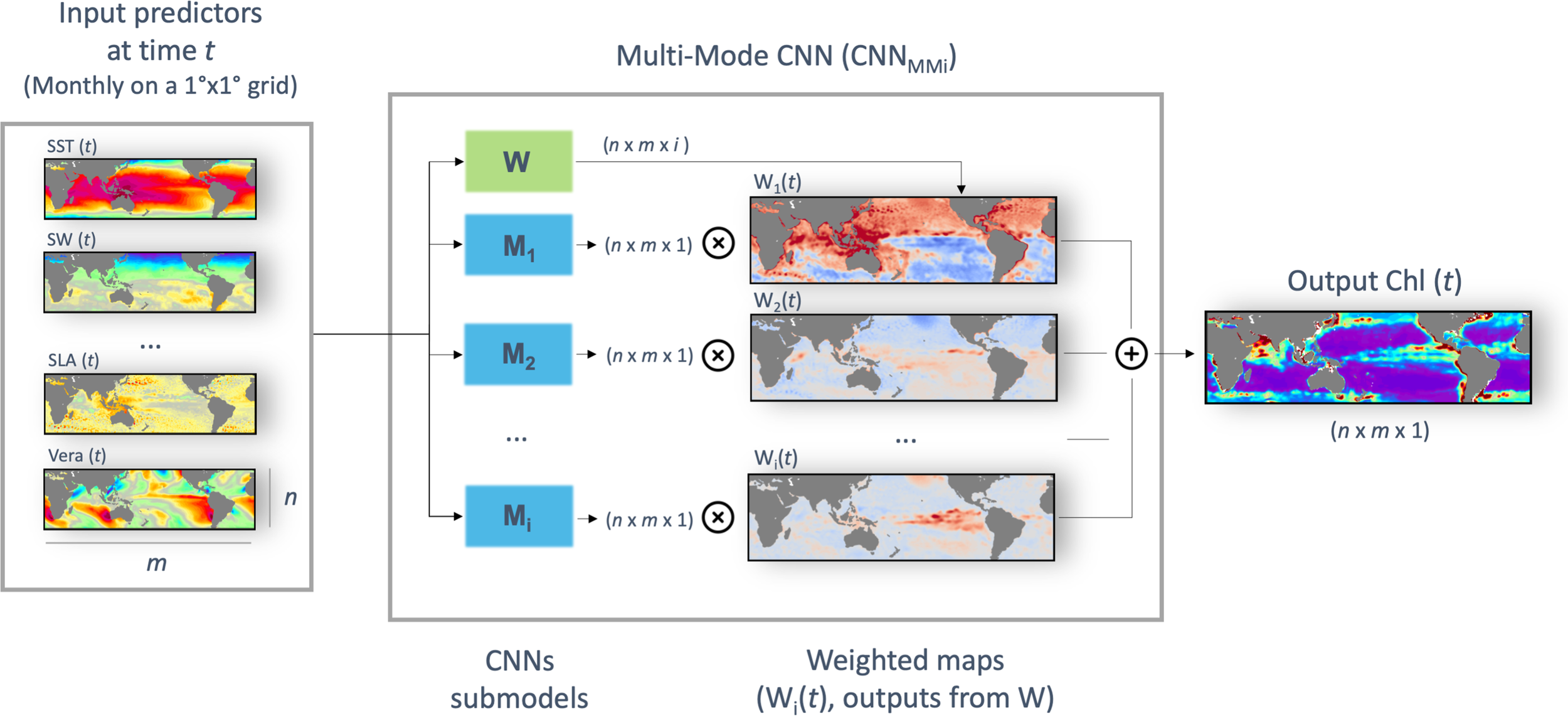
Diagram of the CNNMMi architecture. For a given set of input 2D predictors, each of size n x m, i outputs of size n x m x 1 are computed from the i CNN submodels (Mi). Those are spatially weighted according to the i dynamic probability maps outputted at each time t from the W spatial attention module, and summed to obtain the output Chl 2D field.
2.4 Learning settings
For evaluation purposes, the whole database is split into three independent datasets to train, validate and test the deep-learning schemes. We consider non-overlapping time periods for each dataset as sketched in Figure 2: the training is performed over [2003-2010], the validation dataset covers [1998-2001] to monitor the generalization performance of the models during the training phase and select models’ parameters through sensitivity tests, and reconstructed Chl are compared to satellite Chl over [2012-2015] (i.e., the test time-period). Years 2002 and 2011 are discarded so that the training, test and validation datasets are not auto-correlated. This configuration delivers long-enough test time periods to assess the seasonal and interannual timescales of interest (i.e., El Niño Southern Oscillation - ENSO). It also defines time periods during which the number of ocean color sensors remains the same in the OC-CCI dataset (Sathyendranath et al., 2019) to avoid confusions between possible Chl variations due to switch in sensors or occurring in nature (Gregg et al., 2017).
Figure 2
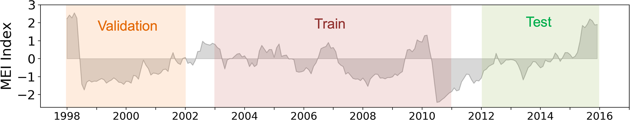
Time-series of the MEI. The validation, training and test time periods used to compare the implemented regression models’ performances are indicated as orange, red and green filled sections, respectively.
We train all models using a Mean Squared Error (MSE) loss and Adam optimizer (Kingma and Ba, 2014). The MLP is trained over 200 epochs with a learning rate of 10-4 and a dropout of 0.15. The CNNs and CNNMMi are trained over 500 epochs with an initial learning rate of 0.001 that is decreased to 0.0001 at the 400th epoch to stabilize the training. Dropout values of 0.15 and 0.35 are used for the CNN1 and CNNMMi, respectively, to prevent overfitting (Srivastava et al., 2014)(see respective learning curves in Figure S3). Hyperparameters settings were chosen according to sensitivity tests summarized in (Supplemental Table S1).
During each training run, we assess the score of the trained model on the validation dataset at the end of each epoch and save the one with the best score. We implement all models using Python with the Pytorch library. We run numerical experiments with a GPU NVIDIA Tesla T4 with 32Go of RAM. As recommended by many ethics’ guidelines for developers (Vinuesa et al., 2020; Ryan and Stahl, 2021; Taddeo et al., 2021), we also report the carbon footprint of the training phase of each model using the Carbontracker Python library (Anthony et al., 2020). Our computing server is located in France, with a detected averaged carbon intensity of 294.21 gCO2/kWh.
2.5 Evaluation framework
We consider the following three quantitative metrics for evaluation purposes: the root-mean-square error (RMSE, Eq. 2), the coefficient of determination (R2, Eq. 3) and the linear regression slope are used to compare the reconstructed log(Chl) times series vs. OC-CCI satellite observations:
with N the number of samples, σ the standard deviation and the horizontal bar the time average, both calculated over the considered time period.
Global map of correlation and of normalized RMSE (NRMSE, Eq. 4) of Chl times series vs. OC-CCI satellite observations are also used to assess regional discrepancies:
To estimate the model’s ability to reproduce seasonal and interannual variabilities, an Empirical Orthogonal Function (EOF) analysis is performed as follows. First, the annual (monthly) ChlOC-CCI average is removed from the initial time series to obtain the seasonal (interannual) Chl anomalies which are then normalized with respect to their standard deviations. We project the reconstructed Chl time series onto these seasonal and interannual ChlOC-CCI spatial patterns and the resulting seasonal and interannual temporal patterns (i.e. the principal components, PCs) are compared to those of ChlOC-CCI using Pearson correlation.
For each pixel, the percentage of variance explained by each of the i modes of the multi-mode CNNMMi is derived to assess their relative importance. It relies on (1) successively reconstructing Chl while putting the probability weights of the corresponding mode to zero, and (2) calculating the difference in RMSE that is observed compared to when Chl is inferred with the full model.
From the obtained i percentages of variance Pk, we further compute, for each pixel, the following entropy-based metric H:
It allows us to evaluate to which extent the reconstruction at a given pixel truly results from a multi-mode relationship (large entropy values) or from a single-mode one (low entropy values).
Finally, we also assess the relative importance of each physical predictor to reconstruct Chl using a perturbation-based method as in Kim et al. (2020). From a given CNNMMi, the difference of the RMSE of the predicted Chl when using the initial data vs. randomly shuffled data (both in time and space) for each predictor individually is computed. RMSE differences are normalized so that the relative importance of all the predictors sums up to one for each pixel.
3 Results and discussion
3.1 Performance of the mono-mode CNN vs. MLP baseline
The reconstructed Chl from both the mono-mode CNN1 and the state-of-the-art MLP are compared to satellite Chl over the [2012-2015] test period to assess the added value of convolutions. When the 12 predictors [namely SLA, SST, Uera, Vera, U, V, SW, sin(lat), sin(lon), cos(lon), sin(month), cos(month)] are used, performances obtained with the MLP and CNN1 remain close (Table 2). However, the CNN1 contains almost twenty times less parameters than the state-of-the-art MLP (~100 000 vs. ~1 800 000, respectively), is ten times faster to compute and more than ten times more energy-efficient, supporting that convolutions are better suited to reconstruct Chl.
Table 2
| Predictors | Global scatterplot | Corr. Seas. PC | Corr. Inter. PC | N param | Time computation | Km travelled by car | |||
|---|---|---|---|---|---|---|---|---|---|
| Model | R2 | RMSE | Slope | ||||||
| 12 | MLP | 0.85 | 0.30 | 0.84 | 0.99 | 0.97 | 1 840 000 | 50h13 | 13.5 |
| CNN1 | 0.86 | 0.30 | 0.87 | 0.99 | 0.98 | 99 889 | 5h | 0.95 | |
| 9 (without sin(lat), cos(lon), sin(lon)) | MLP | 0.59 | 0.50 | 0.57 | 0.97 | 0.85 | 1 836 000 | 50h13 | 13.4 |
| CNN1 | 0.80 | 0.35 | 0.77 | 0.99 | 0.94 | 99 457 | 4h53 | 0.93 | |
| 7 (without sin(month), cos(month)) | CNN1 | 0.80 | 0.35 | 0.81 | 0.98 | 0.96 | 99 169 | 4h52 | 0.92 |
| 9 (+ bathymetry + continental binary mask) | CNN1 | 0.84 | 0.31 | 0.85 | 0.99 | 0.95 | 99 457 | 4h54 | 1.04 |
| CNNMM8 | 0.87 | 0.28 | 0.90 | 1.00 | 0.96 | 803 920 | 39h | 8.9 | |
Global performance metrics obtained with the state-of-the-art MLP, CNN1 and CNNMM8 over the [2012-2015] test period.
The R2, RMSE and slope metrics are calculated between the reconstructed log(Chl) and satellite log(ChlOC-CCI). Correlations of seasonal and interannual 1st principal components from EOF analysis are calculated between the reconstructed Chl and satellite ChlOC-CCI. The number of parameters used and the computation time of the training phase (performed over [2003-2010]) are reported, as well as the associated carbon footprints in equivalent km traveled by car. Performance metrics of the proposed multi-mode approach are highlighted in bold.
To avoid learning constraints of time and space, the models are trained removing the spatial coordinates, i.e. on 9 predictors. Results further stress the relevance of convolutional architectures to reconstruct ChlOC-CCI. Indeed, whereas the MLP highly drops in performance (R2 down to 0.59 and RMSE up to 0.5), the CNN1 still presents satisfactory scores (R2 = 0.80 and RMSE = 0.35) (Table 2). These results averaged at global scale are consistent over the three oceanic basins with a higher R2 between ChlOC-CCI and CNN1 than with MLP by 0.23 and 0.24 respectively in the Indian and Pacific oceans and by 0.14 in the Atlantic Ocean (Figure 3 lower row vs. upper row).
Figure 3
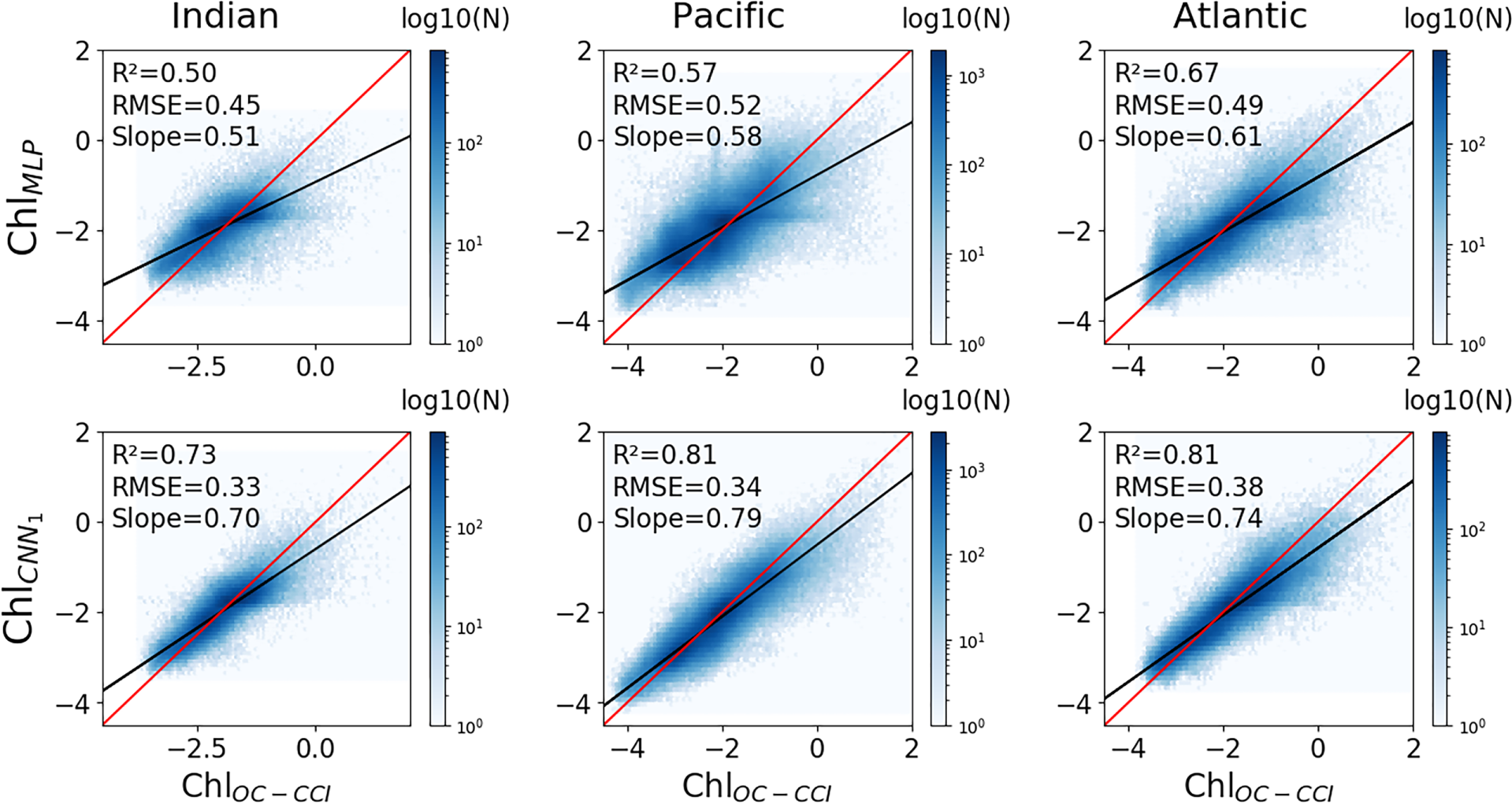
Scatterplots of reconstructed log(Chl) from the MLP (upper row) and CNN1 (lower row) vs. satellite ChlOC-CCI, when explicit geographic predictors (i.e., sin(lat), cos(lon), sin(lon)) are removed from the training phase. Columns correspond to different oceanic basins (left: Indian Ocean, middle: Pacific Ocean, right: Atlantic Ocean). The log of ChlOC-CCI vs. reconstructed log of Chl regression lines are plotted in black and the 1:1 regression lines are plotted in red. Plots are color-coded according to the density of observations.
Interestingly, removing the temporal predictors (i.e., sin(month) and cos(month)) does not reduce the CNN1 performance and even tends to slightly improve it (slope of 0.81 vs. 0.77, and interannual correlation coefficient of 0.96 vs 0.94, Table 2). It suggests that temporal predictors only bring redundant information already included into the seasonally-fluctuating physical fields provided as predictors. This result also suggests that the network benefits from being no longer monthly constrained when interannual time-series are considered. Indeed, learning on periodized months may force the network to learn static seasonal phytoplankton bloom characteristics (e.g., start, duration and amplitude) over several years. Thus, it would impede to correctly account for interannual delays in bloom timing or difference in the length of the growing period (Henson et al., 2009a) that can for instance reach ~10 weeks for major ENSO events (Racault et al., 2012) and that would be otherwise considered through other physical fields such as SST.
The CNN1 is further improved by the addition of two other predictors: the bathymetry and a continental mask. The bathymetry is considered as it would participate to distinguish open ocean ecosystems from coastal ones, where specific processes can occur (shelf break fronts, tidal mixing, river discharge, coastal upwelling, etc) and where the water-leaving radiance measured by ocean color sensors may only partially represent Chl (inorganic particles dominate over phytoplankton concentration). Moreover, as being more spatially resolved than OSCAR data, it is also expected to bring additional information about the ocean circulation (especially concerning the fine-scale dynamic) that is regionally related to the seafloor topography (Gille et al., 2004; Bryan, 2016). The binary continental mask (0 on ocean and 1 on land) is also added because the oceanic predictors are filled over land with data through diffusion (see the data section) inducing that no information on the exact boundary between ocean and land are no longer available. Doing so, results are slightly improved (R2 = 0.84, RMSE = 0.31 and slope = 0.85) and the CNN1 better captures Chl spatial structure in some places as observed over the tropical Atlantic Ocean (Supplemental Figure S2).
3.2 Chl reconstruction improvement from mono-mode CNN1 to multi-mode CNNMM8
Given the overall good performance of the CNN1, we chose this model as a basis to document the impact of multi-modality. With the same 9 predictors, performances of the proposed multi-mode CNNMMi schemes are investigated from 1 to 15 modes. R2 increases from 0.81 up to 0.87 and RMSE decreases from 0.32 down to 0.27 from one to four modes (Figure 4, see Table S2 for details). For both metrics, a plateau is reached from the fourth mode for R2 and the eighth mode for RMSE. Overall, the CNNMM8 model seems to be the best trade-off between performance and computational complexity. Thus, the CNNMM8 is investigated hereafter and compared to CNN1 to further discuss the advantages of the multi-modality.
Figure 4
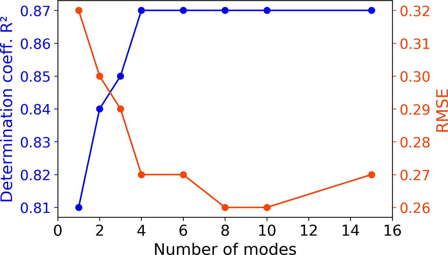
Performance evolution according to the number of modes of the CNNMMi models. Metrics are computed over the [1998-2001] validation period during which model parameters are assessed.
Time averaged satellite ChlOC-CCI over the [2012-2015] test period compares reasonably well with that reconstructed from CNNMM8 (Figures 5A vs. 5B). The CNNMM8 correctly represents the main spatial patterns with, for instance, higher Chl at high latitudes and along the equatorial and eastern boundary upwelling, as well as in the Arabian Sea. The CNNMM8 also captures low Chl in the subtropical gyres delimited by the 0.07 mg.m-3 mean Chl isocontour. The correlation map computed between ChlOC-CCI and CNNMM8 shows values higher than 0.8 over large parts of the global ocean and especially in the subtropical areas (Figure 5C). Conversely, low correlation values, associated in most cases to high NRMSE (Figure 5D), can be observed at higher latitudes than 40° and in the eastern and tropical part of the Pacific Ocean oligotrophic gyres. This can be due to several factors. In some places, the spatio-temporal resolution (i.e., monthly on a 1° grid) used in the present study may be too coarse to capture the overall Chl variability. In particular, this would mainly explain the lack of correlation observed in the tropical southeastern and northwestern Pacific where the dominating timescales of Chl variability have been very recently reported to be below 30 days (Jönsson et al., 2023; see their Figure 7B). This may also explain part of the Chl underestimation observed in highly energetic areas with mesoscale and sub-mesoscale eddies (<100 km scales) that may impact phytoplankton along dynamical fronts (Lévy et al., 2018). This component of the ocean dynamics might not be sufficiently resolved here, as along the Gulf Stream, the Kuroshio and Agulhas currents and in subantarctic waters along the Antarctic Circumpolar Current (Frenger et al., 2018). In addition, the list of predictors that we used is not exhaustive and variables representative of some biogeochemical and physical mechanisms may be missing. For instance, terrigenous inputs at the mouths of large rivers (driven by precipitations) supply nutrient rich waters which are not considered in our predictors. In addition, ocean color observations in these regions may rather reflect suspended particles and colored dissolved organic matter (respectively SPM and CDOM) rather than Chl. This could explain the high NRMSE values observed along the Amazon, the Congo and Kunene rivers. More generally, the predictors we used in this study cannot account for some ocean color sources of uncertainties (e.g., atmospheric conditions, solar zenith angle, properties of the sensors, etc), so potentially biased Chl values cannot be fully reproduced by the networks. Moreover, biological effects such as zooplankton grazing (the so-called top-down control), which are not directly accounted for by any of our predictors, may also regionally inhibit the signature of phytoplankton growth on satellite observations, especially at high latitudes. Proxy of iron supply in the open ocean from other external sources, such as dust deposition or hydrothermal vents, are also missing among our predictors. This can limit the ability of our network to distinguish areas of different nutrient (co-)limitations (Moore et al., 2013) and to account for phytoplankton responses driven by the dynamics of these sources, especially in iron-limited High Nutrient Low Chlorophyll (HNLC) regions. As such, one part of the low correlations observed in the eastern tropical Pacific could come from the role played by dust deposition in altering the timing and amplitude of ENSO-related phytoplankton response (Lim et al., 2022a). This could also partly explain low correlations values observed in the northwestern Pacific (Meng et al., 2022), or high NRMSE values observed in the northern Arabian Sea where dust deposition would play a key role in controlling phytoplankton bloom amplitude (Guieu et al., 2019).
Figure 5
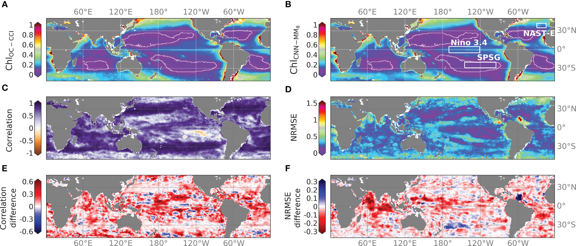
Time averaged (A) ChlOC-CCI and (B) CNNMM8 (in mg.m-3) over [2012-2015]. Oligotrophic gyre boundaries are delimited by the 0.07 mg.m-3 mean Chl isocontour superposed in white. (C) Correlation and (D) NRMSE of ChlOC-CCI vs. CNNMM8 over the same time-period. (E) Correlation and (F) NRMSE differences between CNNMM8 and ChlCNN1 over the same time period. NB: the colorbar is reversed for the NRMSE difference when compared to the correlation difference to highlight in red where the Chl reconstruction with CNNMM8 is improved.
Mean difference maps between CNNMM8 and CNN1 in terms of correlation and NRMSE with ChlOC-CCI illustrate that the CNNMM8 improves correlations over most of the global ocean (in red in Figure 5E). Differences higher than 0.3, and that can exceed 0.6, appear in the tropical zone between 20°S and 20°N (Figure 5E) where Chl are not well reconstructed with the CNN1 (Figure S4). Subtropical areas that already show high correlations with the CNN1 model led to lower differences (yet show no degradation) in the correlation scores. The analysis is a bit more contrasted for the NRMSE metrics. NRMSE values are also improved by the CNNMM8 over most of the global ocean (in red in Figure 5F). However, the NRMSE is deteriorated (in blue) in several regions of the ocean, reaching values up to 0.5 around the Amazon River plume, and up to 0.3 at the mouths of the Congo and Kunene rivers off the coast of Angola, although correlations are improved when multi-modality is introduced. The use of a multi-mode CNN, whose learning is expected to be more regionally focused than a CNN1, might increase the NRMSE in these regions, where Chl variability might rather reflect SPM and CDOM variability whose related predictors are missing.
To illustrate the ability of the CNNMM8 to better capture regional processes than CNN1, the improvement in reconstructed Chl for specific regions when the CNN1 is trained regionally vs. the CNN1 and CNNMM8 trained at global scale is investigated. The CNN1 trained regionally is expected to better learn regional processes than the CNN1 trained over the global ocean (Fourrier et al., 2020). Table 3 shows the performance metrics obtained for two different BGCPs, a productive vs. an oligotrophic region: the Ninõ 3.4 region [5°N–5°S; 120°W–170°W] and the ultra-oligotrophic part of the South Pacific Subtropical Gyre (SPSG, [20°S–30°S; 95°W–145°W]). They present contrasting responses to the regional learning process. The Niño 3.4 region displays a significant potential for performance improvement as shown by the improvement between the globally and locally learnt CNN1, which means that the relationships learnt at global scale are different than those learnt at regional scale. Here, the CNNMM8 reaches those performances and even outperforms the regional CNN1, confirming the hypothesis of a better ability of the multi-mode CNN to reconstruct regional Chl. Contrastingly, in the SPSG region the reconstruction of Chl is already well performed by the globally and locally learnt CNN1 with R2 = 0.85 vs. 0.92, respectively, leaving little room for improvement by the CNNMM8. However, the CNNMM8 allows reduction of the NRMSE. Thus, in both regions, the CNNMM8 outperforms the regionally trained CNN1 due to its ability to switch between different modes while it is less prone to overfitting.
Table 3
| Model | Ninõ 3.4 | SPSG | ||
|---|---|---|---|---|
| R 2 | NRMSE | R 2 | NRMSE | |
| Globally learned CNN1 | 0.28 | 0.17 | 0.85 | 0.14 |
| Regionally learned CNN1 | 0.48 | 0.12 | 0.92 | 0.17 |
| Globally learned CNNMM8 | 0.68 | 0.11 | 0.90 | 0.14 |
Performance metrics obtained between spatially averaged reconstructed Chl and ChlOC-CCI over two contrasted BGCPs: the Ninõ 3.4 region ([5°N–5°S, 120°W–170°W]) and the South Pacific Subtropical Gyre (SPSG, [20°S–30°S; 95°W–145°W]), when the CNN1 is either trained at global scale or regionally, and the CNNMM8 is trained globally.
Best performances are highlighted in bold.
Using the proposed EOF-based analysis, the ability of the CNNMM8 to retrieve the satellite-derived Chl spatio-temporal variability is investigated. The first EOF modes calculated on the seasonal and interannual ChlOC-CCI signal over [2012-2015] are presented in Figure 6 (upper and lower row, respectively). They respectively account for 33.2% and 13.2% of the total variance. Regarding the seasonal variability, the observed spatial patterns depict a clear contrast between the two hemispheres (Figure 6A), reflecting their opposite seasonal cycles. Consistently, the associated PC time-series depicts a sinusoidal signal with a one-year period (black line in Figure 6B). This seasonal variability is well reproduced by both the CNN1 and CNNMM8 models, with correlations of their projected PCs with those of ChlOC-CCI of 0.99 and 1.00, respectively (Figure 6B). Even though the amplitude of the ChlOC-CCI PC was already very well captured by the monomode model, the multi-mode one still allows the correction of the slight underestimation that was observed otherwise.
Figure 6
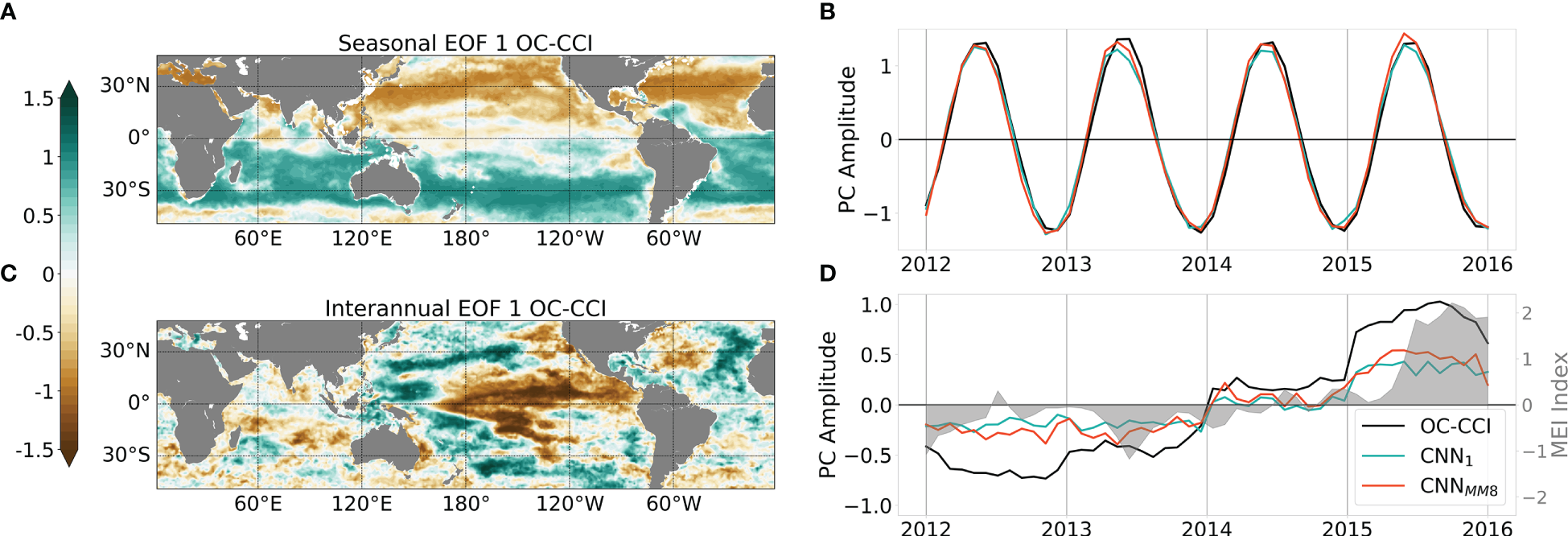
(A) Spatial pattern and (B) associated principal component (PC, as the black line) of the EOF first mode calculated on seasonal ChlOC-CCI over [2012-2015]. ChlCNN1 and ChlCNN-MM8 PCs obtained from the projection on ChlOC-CCI EOF spatial pattern are reported as the green and orange lines, respectively. (C, D) same as (A, B) but for the interannual signal. In (D), the MEI is reported as the grey shaded area.
Regarding the interannual variability, the first ChlOC-CCI EOF mode illustrates the strong spatio-temporal signature of ENSO events observed in the Pacific Ocean (Figure 6C), with opposite Chl responses to ENSO-related physical anomalies observed in the eastern Pacific compared to the western Pacific (Chavez et al., 1999). The temporal evolution of this first interannual ChlOC-CCI PC is highly related to the MEI (r=0.75, p<0.001) which reaches its maximum during the strong 2015/2016 El Niño event (Figure 6D). Here again, the interannual signal is well represented by CNN1 and CNNMM8 with high correlation coefficients of their PCs with those of ChlOC-CCI (0.95 and 0.96, respectively), although the amplitudes are underestimated. These results stress the ability of the learning-based schemes to inform about the seasonal and interannual variability while it is not explicitly constrained during the training phase. Indeed, neither the training loss nor the architecture exploits time-related information. The underestimation of the interannual signal may be related to processes not considered, either related to the predictors (e.g. rivers inputs of nutrients, dust, land wildfire …) or to unresolved spatio-temporal scales. For instance, some discrepancies in the patterns of respective interannual EOF modes 1 can be observed in the Indian ocean and in the north Atlantic ocean (Figures S5B, D, F) where atmospheric dust inputs are most important (Jickells et al., 2005). Other sources of error can arise from differences between the training and the test periods chosen for this study. Beyond differences in the amplitude of ENSO events observed during those periods, different types of ENSO [Eastern Pacific (EP) versus Central Pacific (CP)] have also been reported. Thus, our training period [2003-2011] mainly hosts CP events, whereas the strong 2015/2016 El Niño event is usually classified as an EP event, with different processes and related impact on primary production (Radenac et al., 2012; Racault et al., 2017). Finally, delayed effects of climate modes have been very recently shown to influenced Chl in large parts of the ocean (see Figure 6 of Lim et al., 2022b), and especially in the eastern tropical Pacific one, whereas time-lags are not considered into our model.
3.3 Emergence of coherent spatio-temporal distribution of modes
The main advantage of the multi-mode CNN is the ability of its different sub-models to regionally specialize during the training phase. The training of the network benefits from all the sub-models that activate differently in various parts of the ocean. Maps of the percentage of variance explained by each mode of the CNNMM8 are computed over [2012-2015] (Figures 7A–H). This resulting regionalization, even if presenting some slight modifications of their spatial imprints, are quite consistent from one run to another. These percentages can regionally exceed 30% of the total variance for some modes in specific regions, such as in the three oligotrophic gyres of the southern hemisphere (mode 1), and, to a lesser extent, in those of the northern one (modes 2 and 3). These high variances which predominate for specific modes correspond to low values of entropy (the lower the entropy is, the more a specific mode dominates the signal: purple areas in Figure 7I). The percentages of variance of the remaining oceanic regions are distributed in a more balanced way between a larger number of modes (higher entropy, Figure 7I), but still present some regional variations.
The eight sub-models thus depict some clear, coherent and non-random spatial patterns. Figure 7J synthetizes areas over which the different modes dominate, depicting for each pixel the mode that presents the maximum of explained variance. At first glance, there is a zonal spatial distribution of the modes in agreement with the original BGCPs distribution from Longhurst (1995). It partly results from latitudinal variations in physical forcing and leads to distinguishing what is called the “westerly winds domain” from the “trade wind domain” in the open ocean, whose seasonal changes in MLD are driven by different processes. The first one is reported to extend from the equator to ~30° of latitude, whereas the second one corresponds to mid-latitude areas. From the trained CNNMM8, mode 7 mostly activates at higher latitudes than ~30°N/°S (in blue in Figure 7J), whereas mode 6 mainly activates at low-latitude. The first mode highly matches the three southern hemisphere oligotrophic gyres whereas the second and third modes coincide with the two gyres of the northern hemisphere. The spatial distribution of the three remaining modes (i.e., 4, 5 and 8) fits regions with specific oceanographic dynamics. Indeed, mode 4 (in red in Figure 7J) principally corresponds to areas of wind-induced coastal upwellings, as the Peru, Canary and Benguela areas and to a lesser extent to the California one, as well as to the Pacific and Atlantic equatorial upwelling. Mode 5 (in orange, Figure 7J) seems to stand for the mid-latitude highly dynamical parts of the ocean, that is to say the Gulf Stream and the Kuroshio currents. Finally, mode 8 (in yellow, Figure 7J) potentially highlights the Pacific frontal areas such as the Transition Zone Chlorophyll Front (Polovina et al., 2001) or the boundary between the equatorial Pacific high nutrient low chlorophyll (HNLC) area and the subtropical gyres.
Another feature of the multi-mode CNN is the ability of the sub-models to be variably activated over time. When considering two BGCPs with contrasting entropy such as the eastern North Atlantic Subtropical Gyre (NAST-E, [35°N–42°N; 15°W–30°W]) and the already mentioned SPSG (delimited on Figure 7J) it appears that the percentages of variance explained by each mode, spatially averaged over their respective areas, present contrasted temporal patterns (Figure 8). For instance, clear seasonal patterns emerge in the NAST-E (Figure 8A). The activation of the 7th mode (in light blue) occurs seasonally (with some inter-annual variability) with a maximum in November/December and a smaller secondary peak in April before starting to decrease. Then, the percentage of variance explained by modes 3 and 6 (in garnet and gray, respectively) increases in turn, followed by mode 2 (in green). The strong seasonal cycle observed here is consistent with the seasonal phytoplankton blooms reported in the North Atlantic. Contrastingly, in the SPSG one mode totally prevails over the others and does not display a clear seasonal cycle (purple line in Figure 8B). This strong dominance is also highlighted in Figures 7A, J and in the entropy map (Figure 7I). These results show that the learned modes vary in space but also in time and that they can be variably activated according to the variations of the physical predictors.
Figure 7
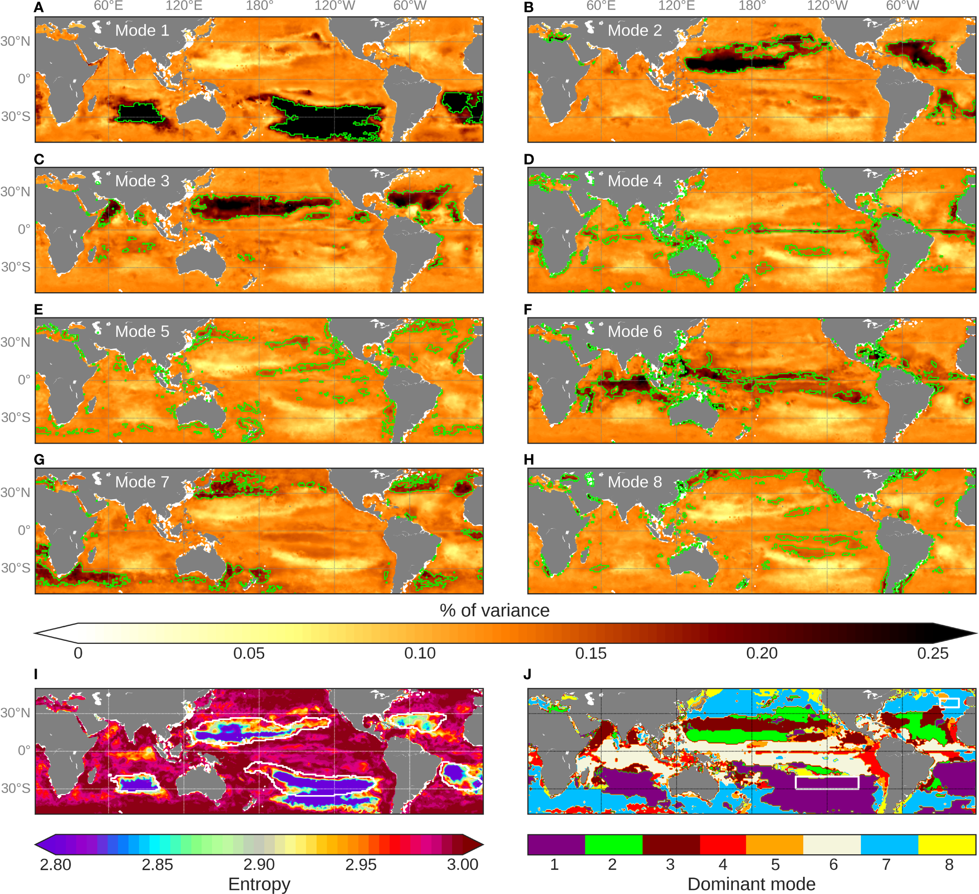
(A–H) Percentages of variance explained by each of the 8 modes of CNNMM8. Isolines of percentile-90 of the values are superposed in green. (I) Entropy characteristics computed from the above percentage of variance. Oligotrophic areas (with mean Chl < 0.07 mg.m-3 calculated over [2012-2015]) are delineated as white isocontours. (J) Spatial distribution of the modes explaining the highest percentage of variance.
Figure 8
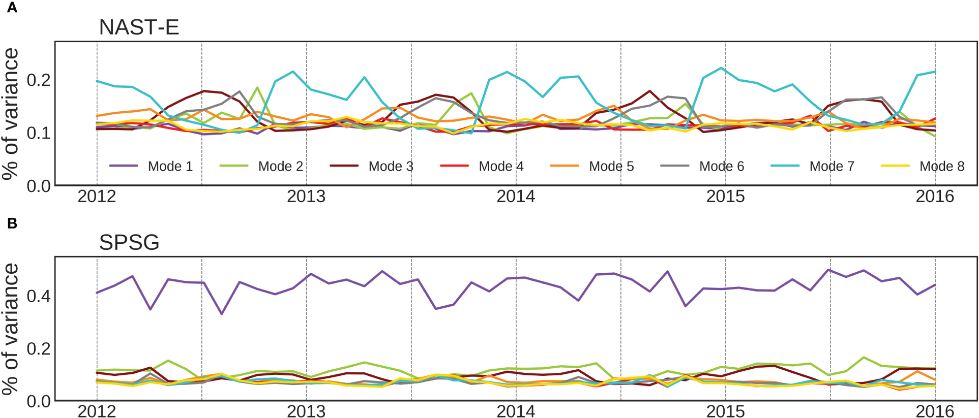
Temporal evolution of the percentages of variance explained by the 8 modes of the CNNMM8 in two BGCPs with contrasting entropy: (A) in the eastern North Atlantic Subtropical Gyre (NAST-E, [35°N–42°N; 15°W–30°W]) and (B) in the SPSG ([20°S–30°S; 95°W–145°W]). The colors correspond to the modes as in Figure 6J.
3.4 Predictors’ relative importance in Chl reconstruction according to the modes
Using the perturbation-based method described in the last paragraph of Section 2.5, here we provide an insight in the relative importance of the physical predictors to reconstruct satellite-derived Chl. Histograms in Figure 9 show the normalized distribution along with the relative importance of each predictor in areas characterized by one dominant mode (i.e. the areas reaching the 90th percentile of variance, delimited by the green lines in Figures 7A–H), over the [2012-2015] test period. Those histograms illustrate that the different modes specialize by learning specific relationships between Chl and the physical predictors, implying possible different physical-biogeochemical interactions and dominant mechanisms. This is especially obvious with regards to the SST for which the eight histograms display various distributions. Those appear to be in general agreement with known physical-biogeochemical processes, but also highlight some unexpected while plausible relationships.
Figure 9
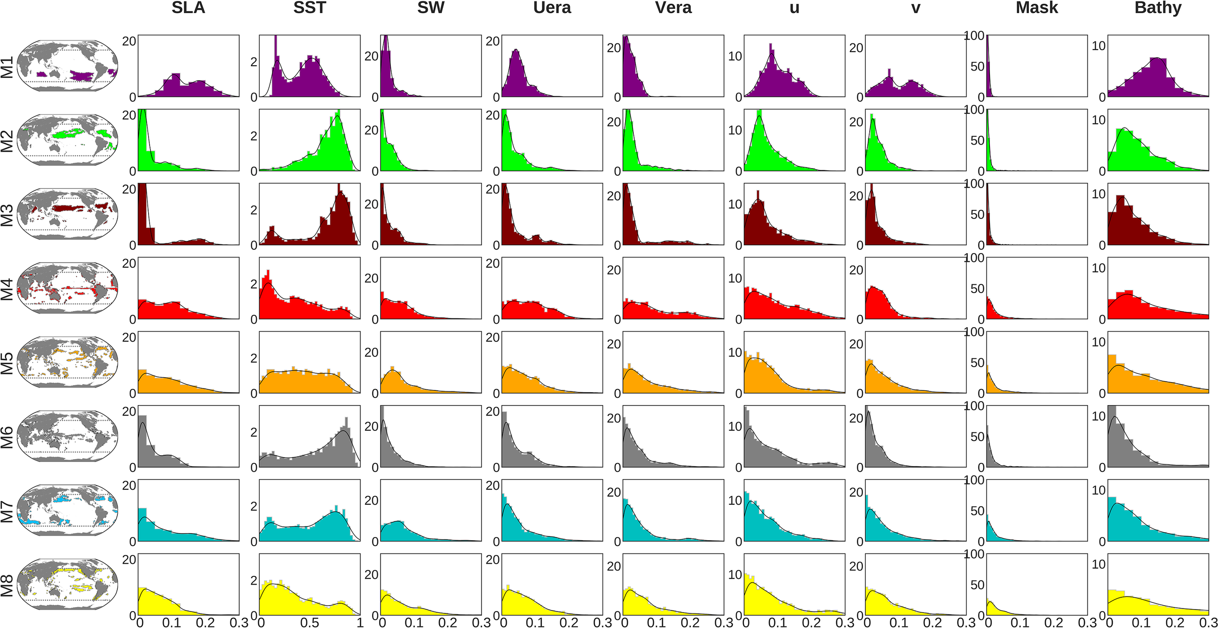
Normalized distribution (y-axis) of the relative importance of each predictor (x-axis) computed over the percentile-90 area for each mode. NB: the scale on the x-axis is homogeneous across all the variables but SST.
As expected and already noted in a previous machine learning based study (Martinez et al., 2020b), SST has the strongest relative importance when compared to other physical predictors in all mode-associated regions (NB: the scale on the x-axis in Figure 9 differs for SST when compared to the other predictors). However, this relative importance is particularly striking in the subtropical gyres of the northern (modes 2 and 3) and southern (mode 1) hemispheres, and in some of the equatorial areas (mode 6) where most of the pixels reach a relative value higher than 0.5. Yet, a maximum/peak of occurrence around 0.7 is reached only for modes 2, 3 and 6. In those latter regions representing (i) the northern subtropical gyres and (ii) the equatorward boundaries of the northern and southern boundaries subtropical gyres, the strong dominance of SST as a predictor is consistent with the SST-Chl inverse relationship reported at global scale in literature (e.g., Behrenfeld et al., 2006; Martinez et al., 2009). Indeed, in the permanently stratified ocean which is nutrient-limited, SST variability is a proxy of vertical mixing variability and thus of the potential uplift of nutrients within the euphotic zone (Signorini et al., 2015).
Interestingly, this statement slightly differs for the southern oligotrophic gyres (mode 1) where the SST importance is weaker (but still dominant) than in the northern gyres (modes 2 & 3). On the contrary, other predictors such as SLA and surface currents (U, V) seem to have a greater relative importance in the southern gyres than in the northern ones. Counterintuitively, it suggests that some of the mechanisms that are at play in the oligotrophic gyres would be different between the two hemispheres. One hypothetic explanation may come from the possible stronger iron limitation in the southern hemisphere (Moore et al., 2001), resulting in a decoupling between the vertical inputs of macro-nutrients (e.g. NO3, PO4) and the phytoplankton local growth, thus minimizing the imprint of the SST-Chl inverse relationship characteristic of the northern hemisphere gyres. Considering the lack of vertical inputs of the limiting nutrients, lateral transport of tracers (nutrients and phytoplankton) near transition zones surrounding the gyres may thus be of greater relative importance in the southern hemisphere, which is consistent with the greater importance of the SLA and currents. The double peak SST distribution in mode 1 could then be interpreted as one characteristic of the gyres [related to the vertical input of nutrients and common to the southern and northern gyres (Signorini et al., 2015)] and one related to the lateral transport of tracers mostly at play in the southern gyres. Consistently, for both mode 1 and mode 3, the smaller relative importance of SST occurs where the relative importance of surface currents (U, V) is larger (not shown), the first peak of low SST importance observed for mode 3 corresponding to the Arabian Sea area.
For the other modes (4, 5, 7 and 8) which correspond to more productive regions (e.g. mode 4 highlights equatorial and coastal upwelling regions) SST, while still dominating, appears to be of weaker relative importance than in the gyres. In addition, the other predictors’ relative weights are more uniformly distributed. This suggests that a significant part of the Chl variability is not explained by processes affecting the SST but is rather related to a complex interaction of processes whose signatures are embedded in other predictors (e.g. lateral currents, light, winds).
Overall, Figure 9 shows that the multi-mode CNN approach may give mechanistic insights on the functioning of specific ocean provinces. Hypothesis drawn from such analysis may therefore be further tested using for example mechanistic numerical models.
4 Discussion and perspectives
CNNs have been widely used these last years in geosciences to leverage the spatial dimension of datasets, and their ability to capture spatial patterns have been largely demonstrated (Makantasis et al., 2015; Shen, 2018; Brodrick et al., 2019; Kattenborn et al., 2021). Consistently, our results confirm their relevance to reconstruct phytoplankton spatio-temporal distribution from physical predictors without using any explicit geographical predictors (i.e., latitude and longitude). Compared to previous studies based on CNNs, our study goes further and provides a more efficient method to manage spatio-temporal heterogeneities. This is one of the main limitations of CNNs, and deep learning models in general, when dealing with environmental variables (Bai et al. 2016; Reichstein et al., 2019; Yuan et al., 2020), especially in a highly dynamical environment such as the ocean. Introducing a multi-mode CNN, we showed that the network can identify different areas over which the learning phase can be regionally optimized. The sub-models have been shown to specialize on physically-consistent regions and thus to better capture regional processes. Such kind of neural network architectures have been previously proposed to tackle the merging of data from various sensors and/or spatio-temporal resolutions (Martínez and Yannakakis, 2014; Yang et al., 2016; Melotti et al., 2018; Ienco et al., 2019; Joze et al., 2020; Zhang et al., 2022). However, to our knowledge, no studies have been done to apply them to regionalization issues. This approach focusing on regional mechanisms converges to recent deep learning architecture built on self-attention processes such as Transformers (Dosovitskiy et al., 2020), but are cheaper in terms of computing cost.
The multi-mode CNN not only allows a better simulation of the chlorophyll concentration spatio-temporal variations, but it also improves the network interpretability, which is of particular interest in the Earth science field as it can allow one to find new unexpected relationships among data. Some post-hoc explanation methods [i.e., once the model is already trained (Fan et al., 2021; Xie et al., 2020)] specifically designed for CNNs, and which are still heavily under-exploited in Earth sciences, may have been considered to go further in the network interpretability (Ras et al., 2022). For instance, Ham et al. (2019) computed heatmaps or Class Activation Maps (CAM, Zhou et al., 2016) from a CNN to analyze which parts of the global ocean contribute the most to the prediction of El Niño events. Zeiler and Fergus (2014) also proposed a way to access and visualize how much information from input data is processed according to the different network layers of CNNs. However, these latter methods do not allow one to optimize the regional learning nor to provide some interpretability from the model outputs, which are both specificities of our multi-mode CNN. Optimizing, during training, specifically designed explanations is what the so-called intrinsic methods aim to do. This is one of the advantages of the proposed multi-mode CNN compared to the mono-mode.
Here, we took advantage of both the intrinsic explainable methods and post-hoc diagnostics to increase the interpretability. Indeed, in the present study, the intrinsic multi-modality shows some consistency in the learning of the eight modes with the spatio-temporal variations of the ocean dynamics, which is somehow expected to be reflected in the variations of the phytoplankton biomass. Applying a basic post-hoc perturbation-based method to the CNNMM8 allowed us investigating the relative importance of the predictors (as illustrated in Figure 9). Other post-hoc methods shedding light on features that drive the model’s decision would deserve to be investigated and compared with one another. For instance, the Shapley Additive exPlanations (SHAP) method (Lundberg and Lee, 2017), which can be applied to any kind of neural networks, measures the effects of an input perturbation on the network’s output to retrieve the relative importance of each predictors (Padarian et al., 2020; Betancourt et al., 2022; Pauthenet et al., 2022). This method would allow consideration of interdependencies between variables, whereas removing them one by one, as did in our study, may not be optimum.
Multi-mode CNN results are promising even if some strategies could further improve the performance of the Chl reconstruction. From the architecture point of view, the addition of pooling layers, especially for the W attention module (see Figure 1), may allow a better consideration of large-scale spatial structures and thus of the regionalization of the different modes. Coupling the CNN sub-models with Recurrent Neural Networks (RNNs) should help accounting for temporal dynamics/time history with a more sophisticated way than if adding time-lags as predictors within our current architecture. Indeed, while instantaneous environmental fluctuations are thought to explain much of the observed phytoplankton temporal variability, time-lag responses of weeks to a few months would also be expected (Ji et al., 2010; Feng et al., 2015; Schollaert Uz et al., 2017; Lim et al., 2022b). This would arise from biological processes mainly, such as dormancy and reproduction (Ji et al., 2010), or ecological interactions as species competition or grazing pressure (Feng et al., 2015). Assessing their own impact on the Chl reconstruction using models that take into account temporal dependencies is certainly worth doing and would deserve a dedicated study but was beyond the scope of this paper. Moreover, while the current network learns different sub-models on specific areas (spatial attention), sub-models could also learn according to different temporal periods (temporal attention). In addition, the current architecture could be easily adapted to learn from predictors with different higher spatio-temporal resolutions. This may improve the Chl reconstruction performance by considering processes currently not resolved with the actual monthly dataset averaged on a 1° grid, such as the mesoscale ocean dynamics or high frequency wind events. This would also enable a better assessment of the impact of finer scale dynamics on Chl low-frequency variability at global scale.
New predictors should also be considered in upcoming studies to stand for a wider range of processes, as mentioned in Section 3.2. Aerosol Optical Depth (AOD) observations could help to account for the sporadic supply of nutrients into the ocean from atmospheric deposition, such as dust-derived iron that can play a significant role on interannual phytoplankton dynamics in some regions (Letelier et al., 2019; Lim et al., 2022a; Meng et al., 2022). Precipitations could help to distinguish wet from dry dust deposition, known to present different iron solubility (Fan et al., 2006), a proxy of iron bioavailability (Schulz et al., 2012). In situ water column data provided from Argo floats could also be considered to better represent the MLD variability rather than using surface proxy only. However, one drawback to fix is that it would reduce the length of available time series of more than 10 years (a sufficient data coverage is not expected before the 2010’s). Chl is a proxy of phytoplankton biomass, and other underlying processes can be reflected on Chl changes. For instance, in response to changes in light conditions, phytoplankton cells can adjust their intracellular Chl so that Chl changes may be rather related to photoadaptation than to biomass. Thus, reconstructing the ratio between Chl and particulate backscattering coefficient [bbp, related to the size particles, Loisel et al., 2002] would deserve to be investigated in future studies. Here we used SW as a proxy of PAR, whereas SW spatiotemporal changes may not always reflect PAR variability due to strong absorption by water vapor, ozone, and clouds outside the PAR spectral range (Chou and Suarez, 1999). Yet, not considering the spectral form of incident radiation can lead to large errors in modeling oceanic primary production (Sathyendranath et al., 1989; Frouin et al., 2018). Sensitivity tests concerning the use of SW as a proxy of PAR should be carried out in the future, for example by comparing the results obtained here with those obtained using PAR products from radiometric observations or reanalysis data (e.g., MERRA-2). Finally, considering uncertainties of the different products used (either for the physical predictors or for the reference satellite-derived Chl) would deserve to be investigated. When available, using pixel-by-pixel estimates of uncertainties as inputs of the network may, for example, allow to give less importance on the learned relationships between predictors and Chl where data quality is lower. In addition, using metrics of performance that include ocean color uncertainties would be useful to distinguish errors that arise in our reconstructions due to such uncertainties from those due to our network architecture and/or used predictive input data.
Here, we have focused on comparing the ability of different deep learning schemes to simulate phytoplankton variability at seasonal and interannual timescales, and have shown that the proposed approach outperforms previous machine learning models introduced in the literature to achieve this task [namely the MLP, and indirectly the less-performant SVR approach (Martinez et al., 2020b)]. In (Martinez et al., 2020a), the SVR approach was quantitatively compared to a coupled physical-biogeochemical ocean model simulation (NEMO-DFS5.2-PISCES) and was found to better reproduce patterns of satellite-derived Chl trends (but less well captures their amplitudes) as well as its interannual variability. This suggests that the proposed multi-mode CNN would, by extent, also better reproduce some aspects of Chl long-term variabilities than biogeochemical models, appearing as a complementary tool to retrieve past Chl variability. Further work is expected to investigate this point, especially regarding multi-decadal changes in global phytoplankton that were pointed out between the CZCS and SeaWiFS era (Martinez et al., 2009) using historical consistent ocean color dataset built by Antoine et al. (2005). Here, we also suggest that data-driven approaches can be complementary to classical models’ studies to explore mechanisms driving phytoplankton variabilities at large scales. For sure, coupled physical-biogeochemical models, that are built upon explicit formulation of processes governing phytoplankton distribution, undoubtedly remain the most robust and straightforward way to test impacts on primary production of processes that are well understood and well parameterized. However, some unknown processes would be missing, or others would be roughly parameterized so that their impact on primary production would be hard to assess without bias. As an example, large variations of parameterized iron solubility in dust are reported among global ocean biogeochemistry models, and the fixed values used globally doesn’t allow reproducing all the regionally and temporally variability of oceanic dust-derived dissolved iron (Tagliabue et al., 2016). On the contrary, using dust deposition flux as inputs predictors, data-driven methods could give new regards and further clues on their regional impact on phytoplankton biomass without having to explicitly parameterize bio-physical values such as solubility. As another example, deriving information about factors driving the phytoplankton ecosystem structure could be achieved using the proposed multi-mode approach. This could be done by learning and reconstructing the phytoplankton community structure [using for example PHYSAT data (Alvain et al., 2008)] with the actual set of predictors and assessing how their relative importance vary in time and space. Such information is of great importance as phytoplankton taxonomic and size composition strongly determines carbon fluxes (Boyd and Newton, 1995; Guidi et al., 2009).
5 Conclusion
In this study, a new deep learning architecture was proposed to reconstruct surface Chl from oceanic and atmospheric physical predictors in the global ocean. Spatial attention mechanisms (i.e. multi modes) were introduced into a CNN to regionally learn relationships in a preferential way according to the modes. Its performance was evaluated over a fully-independent time period hosting the strong 2015/2016 El Niño event. Both mono and multi-mode CNNs outperformed the previous state-of-the-art MLP schemes to reconstruct spatial and temporal satellite-derived Chl distribution while being computationally more efficient. One other main interest of CNNs is their ability to not need explicit geographical information as predictors (e.g. longitude and latitude) leading to the opportunity to seize BGCPs boundaries evolutions according to climate oscillations. In addition, the multi-mode CNNMM8 allowed us to better capture some regional processes than CNN1 thanks to its modes that can regionally learn specific phytoplankton responses to the physical forcing. The multi-mode CNNMM8 also provided insights into where and when the modes preferentially activate, improving the interpretability of the network. Those activations appeared to be in general agreement with known physical-biogeochemical interactions at global scale. However, they also allowed us to highlight an unexpected difference in the mechanisms at play between the oligotrophic gyres of both hemispheres. Overall, while some biases remain between the reconstructed Chl fields and satellite observations, the proposed multi-mode model is greatly valuable as it offers an interesting perspective to reconstruct phytoplankton biomass over a long time-period and new ways to explore the physical mechanisms at play.
Statements
Data availability statement
The datasets presented in this study can be found in online repositories. The names of the repository/repositories and accession number(s) can be found below: https://www.seanoe.org/data/00807/91910/ and https://github.com/JoanaR/multi-mode-CNN-pytorch.
Author contributions
JR led the study, implemented the neural networks, processed the data and wrote the first draft of the manuscript; JR, RF, EM, TG, LD, and JL contributed to the conception of the research and results analysis; EM, RF, TG, and LD contributed to the improvement of the manuscript. JL contributed to run the regionalized mono-mode CNN and to compute the predictors’ relative importance. EM: funding acquisitions. All authors contributed to the article and approved the submitted version.
Funding
The J. Roussillon PhD grant was funded by the ISblue project, Interdisciplinary graduate school for the blue planet (ANR-17-EURE-0015) and co-funded by a grant from the French government under the program “Investissements d’Avenir. We also thank the French National Program of Spatial Remote Sensing (INSU PNTS) for co-funding this work. The Master 2 internship of J. Littaye was funded by the French National Research institute for sustainable Development (IRD).
Acknowledgments
We would like to thank Anwar Brini for providing his Python program to compute the heat diffusion equation. We also warmly thank two reviewers for their very helpful comments on the manuscript. We also acknowledge the NOAA PSL for providing the NCEP-NCAR Reanalysis 1 data. Thanks to NOAA NCEP EMC CMB GLOBAL Reyn-SmithOIv2 for providing monthly SST data. The authors also acknowledge ECMWF for providing the ERA-Interim reanalysis data set. GEBCO is acknowledged for proving bathymetry data. NASA Physical Oceanography data center for providing OSCAR Data. We acknowledge the project team of Ocean Colour Climate Change Initiative for generating and sharing the merged datasets on chlorophyll-a concentrations.
Conflict of interest
The authors declare that the research was conducted in the absence of any commercial or financial relationships that could be construed as a potential conflict of interest.
Publisher’s note
All claims expressed in this article are solely those of the authors and do not necessarily represent those of their affiliated organizations, or those of the publisher, the editors and the reviewers. Any product that may be evaluated in this article, or claim that may be made by its manufacturer, is not guaranteed or endorsed by the publisher.
Supplementary material
The Supplementary Material for this article can be found online at: https://www.frontiersin.org/articles/10.3389/fmars.2023.1077623/full#supplementary-material
References
1
Ai B. Wen Z. Wang Z. Wang R. Su D. Li C. et al . (2020). “Convolutional neural network to retrieve water depth in marine shallow water area from remote sensing images,” in IEEE Journal of Selected Topics in Applied Earth Observations and Remote Sensing, Vol. 13. 2888–2898.
2
Alvain S. Moulin C. Dandonneau Y. Loisel H. (2008). Seasonal distribution and succession of dominant phytoplankton groups in the global ocean: A satellite view. Global Biogeochemical Cycles22 (3). doi: 10.1029/2007GB003154
3
Anthony L. F. W. Kanding B. Selvan R. (2020). Carbontracker: Tracking and predicting the carbon footprint of training deep learning models. arXiv preprint arXiv:2007.03051. doi: 10.48550/arXiv.2007.03051
4
Antoine D. Morel A. Gordon H. R. Banzon V. F. Evans R. H. (2005). Bridging ocean color observations of the 1980s and 2000s in search of long-term trends. J. Geophysical Research: Oceans110 (C6). doi: 10.1029/2004JC002620
5
Anzai Y. Shimada T. (1988). “Modular neural networks for shape and/or location recognition,” in Int Neural Network Soc First Ann Meeting, Boston, USA.
6
Aubert G. Kornprobst P. Aubert G. (2006). Mathematical problems in image processing: partial differential equations and the calculus of variations Vol. 147 (New York: Springer), 26.
7
Auda G. Kamel M. (1999). Modular neural networks: a survey. Int. J. Neural Syst.9 (02), 129–151. doi: 10.1142/S0129065799000125
8
Azam F. (2000). Biologically inspired modular neural networks (Virginia Polytechnic Institute and State University).
9
Bai Y. Wu L. Qin K. Zhang Y. Shen Y. Zhou Y. (2016). A geographically and temporally weighted regression model for ground-level PM2. 5 estimation from satellite-derived 500 m resolution AOD. Remote Sens.8 (3), 262. doi: 10.3390/rs8030262
10
Beaugrand G. Reid P. C. Ibanez F. Lindley J. A. Edwards M. (2002). Reorganization of north Atlantic marine copepod biodiversity and climate. Science296 (5573), 1692–1694. doi: 10.1126/science.1071329
11
Behrenfeld M. J. O’Malley R. T. Siegel D. A. McClain C. R. Sarmiento J. L. Feldman G. C. et al . (2006). Climate-driven trends in contemporary ocean productivity. Nature444 (7120), 752–755. doi: 10.1038/nature05317
12
Bergen K. J. Johnson P. A. Maarten V. Beroza G. C. (2019). Machine learning for data-driven discovery in solid earth geoscience. Science363 (6433). doi: 10.1126/science.aau0323
13
Betancourt C. Stomberg T. T. Edrich A. K. Patnala A. Schultz M. G. Roscher R. et al . (2022). Global, high-resolution mapping of tropospheric ozone–explainable machine learning and impact of uncertainties. Geoscientific Model. Dev. Discussions15 (11), 4331–4354. doi: 10.5194/gmd-15-4331-2022
14
Bisson K. M. Boss E. Werdell P. J. Ibrahim A. Frouin R. Behrenfeld M. J. (2021). Seasonal bias in global ocean color observations. Appl. optics60 (23), 6978–6988. doi: 10.1364/AO.426137
15
Boyd P. Newton P. (1995). Evidence of the potential influence of planktonic community structure on the interannual variability of particulate organic carbon flux. Deep Sea Res. Part I: Oceanographic Res. Papers42 (5), 619–639. doi: 10.1016/0967-0637(95)00017-Z
16
Boyd P. W. Strzepek R. Fu F. Hutchins D. A. (2010). Environmental control of open-ocean phytoplankton groups: Now and in the future. Limnology oceanography55 (3), 1353–1376. doi: 10.4319/lo.2010.55.3.1353
17
Brodrick P. G. Davies A. B. Asner G. P. (2019). Uncovering ecological patterns with convolutional neural networks. Trends Ecol. Evol.34 (8), 734–745. doi: 10.1016/j.tree.2019.03.006
18
Bryan K. (2016). A review of observations of the effect of bathymetry on ocean circulation in recent decades. Izv. Atmos. Ocean. Phys.52, 341–347. doi: 10.1134/S0001433816040034
19
Cachay S. R. Erickson E. Bucker A. F. C. Pokropek E. Potosnak W. Osei S. et al . (2020). Graph neural networks for improved El Nino forecasting. arXiv preprint arXiv:2012.01598. doi: 10.48550/arXiv.2012.01598
20
Chattopadhyay A. Hassanzadeh P. Pasha S. (2020). Predicting clustered weather patterns: A test case for applications of convolutional neural networks to spatio-temporal climate data. Sci. Rep.10 (1), 1–13. doi: 10.1038/s41598-020-57897-9
21
Chavez F. P. Strutton P. G. Friederich G. E. Feely R. A. Feldman G. C. Foley D. G. et al . (1999). Biological and chemical response of the equatorial Pacific Ocean to the 1997-98 El Niño. Science286 (5447), 2126–2131. doi: 10.1126/science.286.5447.2126
22
Chen L. Zhang H. Xiao J. Nie L. Shao J. Liu W. et al . (2017). “Sca-cnn: Spatial and channel-wise attention in convolutional networks for image captioning,” in Proceedings of the IEEE conference on computer vision and pattern recognition. 5659–5667.
23
Chou M. D. Suarez M. J. (1999). A Solar Radiation Parameterization for Atmospheric Studies. In: Suarez (Hrsg.) Technical Report Series on Global Modeling and Data Assimilation NASA/TM-1999-104606, Vol. 15(Greenbelt: NASA Goddard Space Flight Center). 38 pp.
24
Cooke C. L. Scott K. A. (2019). “Estimating sea ice concentration from SAR: Training convolutional neural networks with passive microwave data,” in IEEE Transactions on Geoscience and Remote Sensing, Vol. 57. 4735–4747.
25
d'Ortenzio F. Antoine D. Martinez E. Ribera d'Alcalà M. (2012). Phenological changes of oceanic phytoplankton in the 1980s and 2000s as revealed by remotely sensed ocean-color observations. Global Biogeochemical Cycles26 (4). doi: 10.1029/2011GB004269
26
Devred E. Sathyendranath S. Platt T. (2009). Decadal changes in ecological provinces of the Northwest Atlantic ocean revealed by satellite observations. Geophysical Res. Lett.36 (19). doi: 10.1029/2009GL039896
27
Dohan K. (2017). Ocean surface currents from satellite data. J. Geophysical Research: Oceans122 (4), 2647–2651. doi: 10.1002/2017JC012961
28
Dosovitskiy A. Beyer L. Kolesnikov A. Weissenborn D. Zhai X. Unterthiner T. et al . (2020). An image is worth 16x16 words: Transformers for image recognition at scale. arXiv preprint arXiv:2010.11929. doi: 10.48550/arXiv.2010.11929
29
ESR (2009). OSCAR third degree resolution ocean surface currents. Ver. 1. PO DAAC, CA, USA. doi: 10.5067/OSCAR-03D01
30
Falkowski P. G. Barber R. T. Smetacek V. (1998). Biogeochemical controls and feedbacks on ocean primary production. science281 (5374), 200–206. doi: 10.1126/science.281.5374.200
31
Fan S. M. Moxim W. J. Levy H. (2006). Aeolian input of bioavailable iron to the ocean. Geophysical Res. Lett.33 (7). doi: 10.1029/2005GL024852
32
Fan F. L. Xiong J. Li M. Wang G. (2021). On interpretability of artificial neural networks: A survey. IEEE Transactions on Radiation and Plasma Medical Sciences5 (6), 741–760. doi: 10.48550/arXiv.2001.02522
33
FAO (2020). The state of world fisheries and aquaculture 2020. sustainability in action (Rome). doi: 10.4060/ca9229en
34
Feng J. Durant J. M. Stige L. C. Hessen D. O. Hjermann D.Ø. Zhu L. et al . (2015). Contrasting correlation patterns between environmental factors and chlorophyll levels in the global ocean. Global Biogeochemical Cycles29 (12), 2095–2107. doi: 10.1002/2015GB005216
35
Fourrier M. Coppola L. Claustre H. D’Ortenzio F. Sauzède R. Gattuso J. P. (2020). A regional neural network approach to estimate water-column nutrient concentrations and carbonate system variables in the Mediterranean Sea: CANYON-MED. Front. Mar. Sci.7, 620. doi: 10.3389/fmars.2020.00620
36
Frenger I. Münnich M. Gruber N. (2018). Imprint of southern ocean mesoscale eddies on chlorophyll. Biogeosciences15, 4781–4798. doi: 10.5194/bg-15-4781-2018
37
Frouin R. Ramon D. Boss E. Jolivet D. Compiègne M. Tan J. et al . (2018). Satellite radiation products for ocean biology and biogeochemistry: needs, state-of-the-art, gaps, development priorities, and opportunities. Front. Mar. Sci.5, 3. doi: 10.3389/fmars.2018.00003
38
Gille S. T. Metzger E. J. Tokmakian R. (2004). Seafloor topography and ocean circulation. NAVAL Res. Lab. STENNIS SPACE CENTER MS OCEANOGRAPHY DIV. doi: 10.5670/oceanog.2004.66
39
Goodfellow I. Bengio Y. Courville A. (2016). “Convolutional networks,” in Deep learning (Cambridge, MA, USA: MIT Press), 330–372.
40
Gregg W. W. Casey N. W. (2007). Sampling biases in MODIS and SeaWiFS ocean chlorophyll data. Remote Sens. Environ.111 (1), 25–35. doi: 10.1016/j.rse.2007.03.008
41
Gregg W. W. Rousseaux C. S. Franz B. A. (2017). Global trends in ocean phytoplankton: a new assessment using revised ocean colour data. Remote Sens. Lett.8 (12), 1102–1111. doi: 10.1080/2150704X.2017.1354263
42
Grimaud G. M. Mairet F. Sciandra A. Bernard O. (2017). Modeling the temperature effect on the specific growth rate of phytoplankton: a review. Rev. Environ. Sci. Bio/Technology16 (4), 625–645. doi: 10.1007/s11157-017-9443-0
43
Guidi L. Stemmann L. Jackson G. A. Ibanez F. Claustre H. Legendre L. et al . (2009). Effects of phytoplankton community on production, size, and export of large aggregates: A world-ocean analysis. Limnology Oceanography54 (6), 1951–1963. doi: 10.4319/lo.2009.54.6.1951
44
Guieu C. Al Azhar M. Aumont O. Mahowald N. Levy M. Éthé C. et al . (2019). Major impact of dust deposition on the productivity of the Arabian Sea. Geophysical Res. Lett.46 (12), 6736–6744. doi: 10.1029/2019GL082770
45
Haidar A. Verma B. (2018). “Monthly rainfall forecasting using one-dimensional deep convolutional neural network,” in IEEE Access, Vol. 6. 69053–69063.
46
Ham Y. G. Kim J. H. Luo J. J. (2019). Deep learning for multi-year ENSO forecasts. Nature573 (7775), 568–572. doi: 10.1038/s41586-019-1559-7
47
He K. Zhang X. Ren S. Sun J. (2016). “Identity mappings in deep residual networks,” in Computer Vision–ECCV 2016: 14th European Conference, Amsterdam, The Netherlands, October 11–14, 2016, Proceedings, Part IV 14. 630–645 (Springer International Publishing). doi: 10.1007/978-3-319-46493-0_38
48
Henson S. A. Beaulieu C. Lampitt R. (2016). Observing climate change trends in ocean biogeochemistry: when and where. Global Change Biol.22 (4), 1561–1571. doi: 10.1111/gcb.13152
49
Henson S. A. Dunne J. P. Sarmiento J. L. (2009a). Decadal variability in north Atlantic phytoplankton blooms. J. Geophysical Research: Oceans114 (C4). doi: 10.1029/2008JC005139
50
Henson S. A. Raitsos D. Dunne J. P. McQuatters-Gollop A. (2009b). Decadal variability in biogeochemical models: Comparison with a 50-year ocean colour dataset. Geophysical Res. Lett.36 (21). doi: 10.1029/2009GL040874
51
Henson S. A. Sarmiento J. L. Dunne J. P. Bopp L. Lima I. Doney S. C. et al . (2010). Detection of anthropogenic climate change in satellite records of ocean chlorophyll and productivity. Biogeosciences7 (2), 621–640. doi: 10.5194/bg-7-621-2010
52
Hornik K. Stinchcombe M. White H. (1989). Multilayer feedforward networks are universal approximators. Neural Networks2 (5), 359–366. doi: 10.1016/0893-6080(89)90020-8
53
Ienco D. Interdonato R. Gaetano R. Minh D. H. T. (2019). Combining sentinel-1 and sentinel-2 satellite image time series for land cover mapping via a multi-source deep learning architecture. ISPRS J. Photogrammetry Remote Sens.158, 11–22. doi: 10.1016/j.isprsjprs.2019.09.016
54
IOCCG (2019). Uncertainties in ocean colour remote sensing. Ed. MélinF. (Dartmouth, Canada: International Ocean Colour Coordinating Group). doi: 10.25607/OBP-696
55
Irwin A. J. Oliver M. J. (2009). Are ocean deserts getting larger? Geophysical Res. Lett.36 (18). doi: 10.1029/2009GL039883
56
Jeon W. Kim J. S. Seo K. W. (2021). Reconstruction of terrestrial water storage of GRACE/GFO using convolutional neural network and climate data. J. Korean Earth Sci. Soc.42 (4), 445–458. doi: 10.5467/JKESS.2021.42.4.445
57
Jetley S. Lord N. A. Lee N. Torr P. H. (2018). Learn to pay attention. arXiv preprint arXiv:1804.02391. doi: 10.48550/arXiv.1804.02391
58
Ji R. Edwards M. Mackas D. L. Runge J. A. Thomas A. C. (2010). Marine plankton phenology and life history in a changing climate: current research and future directions. J. plankton Res.32 (10), 1355–1368. doi: 10.1093/plankt/fbq062
59
Jickells T. D. An Z. S. Andersen K. K. Baker A. R. Bergametti G. Brooks N. et al . (2005). Global iron connections between desert dust, ocean biogeochemistry, and climate. science308 (5718), 67–71. doi: 10.1126/science.1105959
60
Jönsson B. F. Salisbury J. Atwood E. C. Sathyendranath S. Mahadevan A. (2023). Dominant timescales of variability in global satellite chlorophyll and SST revealed with a MOving standard deviation saturation (MOSS) approach. Remote Sens. Environ.286, 113404. doi: 10.1016/j.rse.2022.113404
61
Joze H. R. V. Shaban A. Iuzzolino M. L. Koishida K. (2020). “MMTM: Multimodal transfer module for CNN fusion,” in Proceedings of the IEEE/CVF Conference on Computer Vision and Pattern Recognition. 13289–13299.
62
Kahru M. Gille S. T. Murtugudde R. Strutton P. G. Manzano-Sarabia M. Wang H. et al . (2010). Global correlations between winds and ocean chlorophyll. J. Geophysical Research: Oceans115 (C12). doi: 10.1029/2010JC006500
63
Kalnay E. Kanamitsu M. Kistler R. Collins W. Deaven D. Gandin L. et al . (1996). The NCEP/NCAR 40-year reanalysis project. Bull. Am. meteorological Soc.77 (3), 437–472. doi: 10.1175/1520-0477(1996)077<0437:TNYRP>2.0.CO;2
64
Kattenborn T. Leitloff J. Schiefer F. Hinz S. (2021). Review on convolutional neural networks (CNN) in vegetation remote sensing. ISPRS J. Photogrammetry Remote Sens.173, 24–49. doi: 10.1016/j.isprsjprs.2020.12.010
65
Kim Y. J. Kim H. C. Han D. Lee S. Im J. (2020). Prediction of monthly Arctic sea ice concentrations using satellite and reanalysis data based on convolutional neural networks. Cryosphere14 (3), 1083–1104. doi: 10.5194/tc-14-1083-2020
66
Kingma D. P. Ba J. (2014). Adam: A method for stochastic optimization. arXiv preprint arXiv, 1412.6980. doi: 10.48550/arXiv.1412.6980
67
Kirsch L. Kunze J. Barber D. (2018). Modular networks: Learning to decompose neural computation. Adv. Neural Inf. Process. Syst.31. doi: 10.48550/arXiv.2001.02522
68
Letelier R. M. Björkman K. M. Church M. J. Hamilton D.S. Mahowald N. M. Scanza R.A. et al . (2019). Climate-driven oscillation of phosphorus and iron limitation in the north pacific subtropical gyre. Proc. Natl. Acad. Sci.116, 12720–12728. doi: 10.1073/pnas.1900789116
69
Lewandowska A. M. Boyce D. G. Hofmann M. Matthiessen B. Sommer U. Worm B. (2014). Effects of sea surface warming on marine plankton. Ecol. Lett.17 (5), 614–623. doi: 10.1111/ele.12265
70
Lévy M. Franks P. J. Smith K. S. (2018). The role of submesoscale currents in structuring marine ecosystems. Nat. Commun.9 (1), 1–16. doi: 10.1038/s41467-018-07059-3
71
Lim H. G. Dunne J. P. Stock C. A. Ginoux P. John J. G. Krasting J. (2022a). Oceanic and atmospheric drivers of post-El-Niño chlorophyll rebound in the equatorial pacific. Geophysical Res. Lett.49 (5), e2021GL096113. doi: 10.1029/2021GL096113
72
Lim H. G. Dunne J. P. Stock C. A. Kwon M. (2022b). Attribution and predictability of climate-driven variability in global ocean color. J. Geophysical Research: Oceans127 (10), e2022JC019121. doi: 10.1029/2022JC019121
73
Loisel H. Nicolas J.-M. Deschamps P.-Y. Frouin R. (2002). Seasonal and inter-annual variability of particulate organic matter in the global ocean. Geophys. Res. Lett.29 (24), 2196. doi: 10.1029/2002GL015948
74
Long D. Shen Y. Sun A. Hong Y. Longuevergne L. Yang Y. et al . (2014). Drought and flood monitoring for a large karst plateau in southwest China using extended GRACE data. Remote Sens. Environ.155, 145–160. doi: 10.1016/j.rse.2014.08.006
75
Longhurst A. Sathyendranath S. Platt T. Caverhill C. (1995). An estimate of global primary production in the ocean from satellite radiometer data. J. plankton Res.17 (6), 1245–1271. doi: 10.1093/plankt/17.6.1245
76
Lundberg S. M. Lee S. I. (2017). A unified approach to interpreting model predictions. Adv. Neural Inf. Process. Syst.30. doi: 10.48550/arXiv.1705.07874
77
Makantasis K. Karantzalos K. Doulamis A. Doulamis N. (2015). “Deep supervised learning for hyperspectral data classification through convolutional neural networks,” in 2015 IEEE International Geoscience and Remote Sensing Symposium (IGARSS). 4959–4962 (IEEE).
78
Martinez E. Antoine D. D’Ortenzio F. Gentili B. (2009). Climate-driven basin-scale decadal oscillations of oceanic phytoplankton. Science326 (5957), 1253–1256. doi: 10.1126/science.1177012
79
Martinez E. Antoine D. d'Ortenzio F. de Boyer Montegut C. (2011). Phytoplankton spring and fall blooms in the north atlantic in the 1980s and 2000s. J. Geophysical Research: Oceans116 (C11). doi: 10.1029/2010JC006836
80
Martinez E. Brini A. Gorgues T. Drumetz L. Roussillon J. Tandeo P. et al . (2020a). Neural network approaches to reconstruct phytoplankton time-series in the global ocean. Remote Sens.12 (24), 4156. doi: 10.3390/rs12244156
81
Martinez E. Gorgues T. Lengaigne M. Fontana C. Sauzède R. Menkes C. et al . (2020b). Reconstructing global chlorophyll-a variations using a non-linear statistical approach. Front. Mar. Sci.7, 464. doi: 10.3389/fmars.2020.00464
82
Martínez H. P. Yannakakis G. N. (2014). “Deep multimodal fusion: Combining discrete events and continuous signals,” in Proceedings of the 16th International conference on multimodal interaction. 34–41.
83
McClain C. R. Signorini S. R. Christian J. R. (2004). Subtropical gyre variability observed by ocean-color satellites. Deep Sea Res. Part II: Topical Stud. Oceanography51 (1-3), 281–301. doi: 10.1016/j.dsr2.2003.08.002
84
Mélin F. Hoepffner N. (2011). “Monitoring phytoplankton productivity from satellite–an aid to marine resources management,” in Handbook of satellite remote sensing image interpretation: Applications for marine living resources conservation and management. Eds. MoralesJ.StuartV.PlattT.SathyendranathS. (EU PRESPO and IOCCG), 79–93.
85
Melotti G. Premebida C. Gonçalves N. M. D. S. Nunes U. J. Faria D. R. (2018). “Multimodal CNN pedestrian classification: a study on combining LIDAR and camera data,” in 2018 21st International Conference on Intelligent Transportation Systems (ITSC). 3138–3143 (IEEE).
86
Meng L. Yan C. Zhuang W. Zhang W. Yan X. H. (2021). Reconstruction of three-dimensional temperature and salinity fields from satellite observations. J. Geophysical Research: Oceans126 (11), e2021JC017605. doi: 10.1029/2021JC017605
87
Messié M. Chavez F. P. (2012). A global analysis of ENSO synchrony: The oceans' biological response to physical forcing. J. Geophysical Research: Oceans117 (C9). doi: 10.1029/2012JC007938
88
Yao F. Zhang J. Liu Q. Liu Q. Shi L. Zhang D. et al . (2022). Impact of dust deposition on phytoplankton biomass in the northwestern pacific: A long-term study from 1998 to 2020. Sci. Total Environ.813, 152536. doi: 10.1016/j.scitotenv.2021.152536
89
Micheli-Tzanakou E. (1987). “A neural network model of the vertebrate retina,” in 9th Ann. Conf. IEEE Engineering in Medicine and Biology Society (Boston, MA, USA). 13–16.
90
Moore J. K. Doney S. C. Glover D. M. Fung I. Y. (2001). Iron cycling and nutrient-limitation patterns in surface waters of the world ocean. Deep Sea Res. Part II: Topical Stud. Oceanography49 (1-3), 463–507. doi: 10.1016/S0967-0645(01)00109-6
91
Moore C. M. Mills M. M. Arrigo K. R. Berman-Frank I. Bopp L. Boyd P. W. et al . (2013). Processes and patterns of oceanic nutrient limitation. Nat. Geosci.6 (9), 701–710. doi: 10.1038/ngeo1765
92
Oliver M. J. Irwin A. J. (2008). Objective global ocean biogeographic provinces. Geophysical Res. Lett.35, L15601. doi: 10.1029/2008GL034238
93
Padarian J. McBratney A. B. Minasny B. (2020). Game theory interpretation of digital soil mapping convolutional neural networks. Soil6 (2), 389–397. doi: 10.5194/soil-6-389-2020
94
Pan B. Hsu K. AghaKouchak A. Sorooshian S. (2019). Improving precipitation estimation using convolutional neural network. Water Resour. Res.55 (3), 2301–2321. doi: 10.1029/2018WR024090
95
Patara L. Visbeck M. Masina S. Krahmann G. Vichi M. (2011). Marine biogeochemical responses to the north Atlantic oscillation in a coupled climate model. J. Geophysical Research: Oceans116 (C7). doi: 10.1029/2010JC006785
96
Pauthenet E. Bachelot L. Balem K. Maze G. Tréguier A. M. Roquet F. et al . (2022). Four-dimensional temperature, salinity and mixed layer depth in the gulf stream, reconstructed from remote sensing and in situ observations with neural networks. Ocean Sci.18 (4), 1221–1244. doi: 10.5194/os-18-1221-2022
97
Polovina J. J. Howell E. A. Abecassis M. (2008). Ocean's least productive waters are expanding. Geophysical Res. Lett.35 (3). doi: 10.1029/2007GL031745
98
Polovina J. J. Howell E. Kobayashi D. R. Seki M. P. (2001). The transition zone chlorophyll front, a dynamic global feature defining migration and forage habitat for marine resources. Prog. oceanography49 (1-4), 469–483. doi: 10.1016/S0079-6611(01)00036-2
99
Pyo J. Cho K. H. Kim K. Baek S. S. Nam G. Park S. (2021). Cyanobacteria cell prediction using interpretable deep learning model with observed, numerical, and sensing data assemblage. Water Res.203, 117483. doi: 10.1016/j.watres.2021.117483
100
Racault M. F. Le Quéré C. Buitenhuis E. Sathyendranath S. Platt T. (2012). Phytoplankton phenology in the global ocean. Ecol. Indic.14 (1), 152–163. doi: 10.1016/j.ecolind.2011.07.010
101
Racault M. F. Sathyendranath S. Brewin R. J. Raitsos D. E. Jackson T. Platt T. (2017). Impact of El Niño variability on oceanic phytoplankton. Front. Mar. Sci.4, 133. doi: 10.3389/fmars.2017.00133
102
Radenac M. H. Léger F. Singh A. Delcroix T. (2012). Sea Surface chlorophyll signature in the tropical pacific during eastern and central pacific ENSO events. J. Geophysical Research: Oceans117 (C4). doi: 10.1029/2011JC007841
103
Ras G. Xie N. Van Gerven M. Doran D. (2022). Explainable deep learning: A field guide for the uninitiated. J. Artif. Intell. Res.73, 329–397. doi: 10.1613/jair.1.13200
104
Reichstein M. Camps-Valls G. Stevens B. Jung M. Denzler J. Carvalhais N. (2019). Deep learning and process understanding for data-driven earth system science. Nature566 (7743), 195–204. doi: 10.1038/s41586-019-0912-1
105
Reygondeau G. Cheung W. W. Wabnitz C. C. Lam V. W. Frölicher T. Maury O. (2020). Climate change-induced emergence of novel biogeochemical provinces. Front. Mar. Sci.7, 657. doi: 10.3389/fmars.2020.00657
106
Reygondeau G. Longhurst A. Martinez E. Beaugrand G. Antoine D. Maury O. (2013). Dynamic biogeochemical provinces in the global ocean. Global Biogeochemical Cycles27 (4), 1046–1058. doi: 10.1002/gbc.20089
107
Reynolds R. W. Rayner N. A. Smith T. M. Stokes D. C. Wang W. (2002). An improved in situ and satellite SST analysis for climate. J. Climate15 (13), 1609–1625. doi: 10.1175/1520-0442(2002)015<1609:AIISAS>2.0.CO;2
108
Ronneberger O. Fischer P. Brox T. (2015). “U-net: Convolutional networks for biomedical image segmentation,” in Medical Image Computing and Computer-Assisted Intervention–MICCAI 2015: 18th International Conference, Munich, Germany, October 5-9, 2015, Proceedings, Part III 18. 234–241 (Springer International Publishing). doi: 10.1007/978-3-319-24574-4_28
109
Roussillon J. Fablet R. Gorgues T. Drumetz L. Littaye J. Martinez E. (2022). satellIte phytoplaNkton drivers in the global ocean over 1998-2015 (INDIGO benchmark dataset). SEANOE. doi: 10.17882/91910
110
Ryan M. Stahl B. C. (2021). Artificial intelligence ethics guidelines for developers and users: clarifying their content and normative implications. J. Information Communication Ethics Soc.19 (1), 61–86. doi: 10.1108/JICES-12-2019-0138
111
Sammartino M. Buongiorno Nardelli B. Marullo S. Santoleri R. (2020). An artificial neural network to infer the Mediterranean 3D chlorophyll-a and temperature fields from remote sensing observations. Remote Sens.12 (24), 4123. doi: 10.3390/rs12244123
112
Sathyendranath S. Brewin R. J. W. Brockmann C. Brotas V. Calton B. Chuprin A. et al . (2019). An ocean-colour time series for use in climate studies: the experience of the ocean-colour climate change initiative (OC-CCI). Sensors19, 4285. doi: 10.3390/s19194285
113
Sathyendranath S. Platt T. Caverhill C. M. Warnock R. E. Lewis M. R. (1989). Remote sensing of oceanic primary production: computations using a spectral model. deep Sea research part a. Oceanographic Res. Papers36 (3), 431–453. doi: 10.1016/0198-0149(89)90046-0
114
Sauzède R. Claustre H. Uitz J. Jamet C. Dall'Olmo G. d'Ortenzio F. et al . (2016). A neural network-based method for merging ocean color and argo data to extend surface bio-optical properties to depth: Retrieval of the particulate backscattering coefficient. J. Geophysical Research: Oceans121 (4), 2552–2571. doi: 10.1002/2015JC011408
115
Schollaert Uz S. Busalacchi A. J. Smith T. M. Evans M. N. Brown C. W. Hackert E. C. (2017). Interannual and decadal variability in tropical pacific chlorophyll from a statistical reconstruction: 1958–2008. J. Climate30 (18), 7293–7315. doi: 10.1175/JCLID-16-0202.1
116
Schulz M. Prospero J. M. Baker A. R. Dentener F. Ickes L. Liss P. S. et al . (2012). Atmospheric transport and deposition of mineral dust to the ocean: Implications for research needs. Environ. Sci. Technol.46 (19), 10390–10404. doi: 10.1021/es300073u
117
Shen C. (2018). A transdisciplinary review of deep learning research and its relevance for water resources scientists. Water Resour. Res.54 (11), 8558–8593. doi: 10.1029/2018WR022643
118
Signorini S. R. Franz B. A. McClain C. R. (2015). Chlorophyll variability in the oligotrophic gyres: mechanisms, seasonality and trends. Front. Mar. Sci.2, 1. doi: 10.3389/fmars.2015.00001
119
Srivastava N. Hinton G. Krizhevsky A. Sutskever I. Salakhutdinov R. (2014). Dropout: a simple way to prevent neural networks from overfitting. J. Mach. Learn. Res.15 (1), 1929–1958. doi: 10.5555/2627435.2670313
120
Sun A. Y. Scanlon B. R. Zhang Z. Walling D. Bhanja S. N. Mukherjee A. et al . (2019). Combining physically based modeling and deep learning for fusing GRACE satellite data: can we learn from mismatch? Water Resour. Res.55 (2), 1179–1195. doi: 10.1029/2018WR023333
121
Szeto M. Werdell P. J. Moore T. S. Campbell J. W. (2011). Are the world's oceans optically different? J. Geophysical Research: Oceans116 (C7). doi: 10.1029/2011JC007230
122
Taddeo M. Tsamados A. Cowls J. Floridi L. (2021). Artificial intelligence and the climate emergency: Opportunities, challenges, and recommendations. One Earth4 (6), 776–779. doi: 10.1016/j.oneear.2021.05.018
123
Tagliabue A. Aumont O. DeAth R. Dunne J. P. Dutkiewicz S. Galbraith E. et al . (2016). How well do global ocean biogeochemistry models simulate dissolved iron distributions? Global Biogeochemical Cycles30 (2), 149–174. doi: 10.1002/2015GB005289
124
Vinuesa R. Azizpour H. Leite I. Balaam M. Dignum V. Domisch S. et al . (2020). The role of artificial intelligence in achieving the sustainable development goals. Nat. Commun.11 (1), 233. doi: 10.1038/s41467-019-14108-y
125
Weyn J. A. Durran D. R. Caruana R. (2020). Improving data-driven global weather prediction using deep convolutional neural networks on a cubed sphere. J. Adv. Modeling Earth Syst.12 (9), e2020MS002109. doi: 10.1029/2020MS002109
126
Wilson C. Adamec D. (2002). A global view of bio-physical coupling from SeaWiFS and TOPEX satellite data 1997–2001. Geophysical Res. Lett.29 (8), 98–91. doi: 10.1029/2001GL014063
127
Wilson C. Coles V. J. (2005). Global climatological relationships between satellite biological and physical observations and upper ocean properties. J. Geophysical Research: Oceans110 (C10). doi: 10.1029/2004JC002724
128
Winder M. Sommer U. (2012). Phytoplankton response to a changing climate. Hydrobiologia698, 5–16. doi: 10.1007/s10750-012-1149-2
129
Xie N. Ras G. van Gerven M. Doran D. (2020). Explainable deep learning: A field guide for the uninitiated. arXiv preprint arXiv:2004.14545. doi: 10.48550/arXiv.2004.14545
130
Yang X. Molchanov P. Kautz J. (2016). “Multilayer and multimodal fusion of deep neural networks for video classification,” in Proceedings of the 24th ACM international conference on Multimedia. 978–987.
131
Ye H. Tang S. Yang C. (2021). Deep learning for chlorophyll-a concentration retrieval: A case study for the pearl river estuary. Remote Sens.13 (18), 3717. doi: 10.3390/rs13183717
132
Yu B. Xu L. Peng J. H. Hu Z. Wong A. (2020). Global chlorophyll-a concentration estimation from moderate resolution imaging spectroradiometer using convolutional neural networks. J. Appl. Remote Sens.14 (3), 034520. doi: 10.1117/1.JRS.14.034520
133
Yuan Q. Shen H. Li T. Li Z. Li S. Jiang Y. et al . (2020). Deep learning in environmental remote sensing: Achievements and challenges. Remote Sens. Environ.241, 111716. doi: 10.1016/j.rse.2020.111716
134
Zeiler M. D. Fergus R. (2014). “Visualizing and understanding convolutional networks,” in European conference on computer vision. 818–833.
135
Zhang H. Yao J. Ni L. Gao L. Huang M. (2022). Multimodal attention-aware convolutional neural networks for classification of hyperspectral and LiDAR data. IEEE J. Selected Topics Appl. Earth Observations Remote Sens. doi: 10.1109/JSTARS.2022.3187730
136
Zhou B. Khosla A. Lapedriza A. Oliva A. Torralba A. (2016). “Learning deep features for discriminative localization,” in Proceedings of the IEEE conference on computer vision and pattern recognition. 2921–2929.
Summary
Keywords
Convolutional Neural Networks, attention mechanisms, satellite ocean color, phytoplankton physical drivers, biogeochemical regions, neural networks interpretability, time-series regression, global scale
Citation
Roussillon J, Fablet R, Gorgues T, Drumetz L, Littaye J and Martinez E (2023) A Multi-Mode Convolutional Neural Network to reconstruct satellite-derived chlorophyll-a time series in the global ocean from physical drivers. Front. Mar. Sci. 10:1077623. doi: 10.3389/fmars.2023.1077623
Received
23 October 2022
Accepted
24 February 2023
Published
16 March 2023
Volume
10 - 2023
Edited by
Mark C. Benfield, Louisiana State University, United States
Reviewed by
Bruno Buongiorno Nardelli, National Research Council (CNR), Italy; Robert J. Frouin, University of California, San Diego, United States
Updates
Copyright
© 2023 Roussillon, Fablet, Gorgues, Drumetz, Littaye and Martinez.
This is an open-access article distributed under the terms of the Creative Commons Attribution License (CC BY). The use, distribution or reproduction in other forums is permitted, provided the original author(s) and the copyright owner(s) are credited and that the original publication in this journal is cited, in accordance with accepted academic practice. No use, distribution or reproduction is permitted which does not comply with these terms.
*Correspondence: Joana Roussillon, joana.roussillon@gmail.com
This article was submitted to Ocean Observation, a section of the journal Frontiers in Marine Science
Disclaimer
All claims expressed in this article are solely those of the authors and do not necessarily represent those of their affiliated organizations, or those of the publisher, the editors and the reviewers. Any product that may be evaluated in this article or claim that may be made by its manufacturer is not guaranteed or endorsed by the publisher.