Bayesian geoacoustic parameters inversion for multi-layer seabed in shallow sea using underwater acoustic field

Seabed geoacoustic parameters play an important role in underwater acoustic channel modeling. Traditional methods to determine these parameters, for example, drilling, are expensive and are being replaced by acoustic inverse technology. An inversion method based on Bayesian theory is presented to derive the structure and geoacoustic parameters of a layered seabed in a shallow sea. The seabed was considered a layered elastic medium. The objective of this research was to use the sound pressure detected by underwater acoustic sensors at different positions and to use nonlinear Bayesian inversion to estimate the geoacoustic parameters and their uncertainties in the multi-layer seabed. Specifically, the thickness, density, compression wave speed, shear wave speed, and the attenuation of these two wave speeds were determined. The maximum a posterior (MAP) model and posterior probability distribution of each parameter were estimated using the optimized simulated annealing (OSA) and Metropolis-Hastings sampling (MHS) methods. Model selection was carried out using the Bayesian information criterion (BIC) to determine the optimal model that thoroughly explained the experimental data for different parameterizations. The results showed that the OSA is much more capable of delivering high-accuracy results in multi-layer seabed models. The compression wave speed and shear wave speed were less uncertain than the other parameters, and the parameters in the upper layer had less uncertainty than those in the lower layer.

1 Introduction

Acoustic waves are currently the only means of realizing underwater long-distance detection and communication. When acoustic waves propagating in shallow sea, they will be significantly affected by environment parameters. Moreover, the influence of seabed geoacoustic parameters on acoustic propagation is apparent. Therefore, the accurate inversion of shallow sea geoacoustic parameters is vital. (Benavente et al., 2019). Methods used to determine the seabed’s geoacoustic parameters can be divided into those that rely on direct and indirect measurements (Yin and Hu, 2016). Direct methods mainly involve the acquisition of samples of the seabed substrate by drilling into the seabed. In contrast, acquiring of geoacoustic parameters relies more on the indirect measurement of acoustic inversion techniques. This technology has been widely used to obtain geoacoustic parameters because of its technical efficiency.

Past inversion studies for the acoustic properties of shallow seabed mainly focused on the geoacoustic parameters in the surface seabed, and assumed the seabed to be a liquid medium (Michalopoulou and Gerstoft, 2019). With the development of technology, simply treating the seabed as a liquid medium cannot meet the research needs, also it is urgent to obtain the stratified structure and parameters of the seabed simultaneously and accurately. Since Low-Frequency (LF)/Very-Low-Frequency (VLF) acoustic waves can penetration into the seabed deeply, they are more suitable to be used to obtain the structure and parameters (Yuan et al., 2019). However, there are few related studies at present. Therefore, this paper proposes an algorithm suitable for obtaining the geoacoustic parameters of the elastic seabed with multiple layers. (Zhang et al., 2020)

Geoacoustic parameter inversion represents a strongly nonlinear problem with multiparameter solutions for which an immediate answer is unavailable. Initially, optimization algorithms such as simulated annealing (SA) and genetic algorithm (GA) approaches have been widely used in the field of inversion to solve the error function (Sen and Stoffa, 2006; Zhang et al., 2021). However, the disadvantage of SA and GA algorithms is that they can only provide a set of MAP (Maximum A Posteriori, MAP) values, which is unrealistic for the multi-parameter coupling problem. In fact, because of the high randomness of the sea environment, the measured data inevitably contain systematic and random errors; thus, an uncertainty analysis of the inversion results is essential. It is unreasonable and insufficiently comprehensive to provide only a set of MAP values for optimal solution parameters to obtain the inversion result. The inversion method based on nonlinear Bayesian theory is a global optimization algorithm with roots in interdisciplinary subjects, such as probability theory, applied mathematics, and optimization theory. This algorithm can not only be used to effectively estimate the parameters of the MAP model, but it can also evaluate the uncertainty in the parameter inversion results from a statistical perspective, making it more suitable for meeting the current needs of the research on geoacoustic parameter inversion.

In general, the seabed of the shallow sea environment along the coast has a layered structure with multiple sedimentary layers, and the hardness of this seabed structure increases with the depth of the seabed. The research objective of this study was to determine the sound pressure detected by underwater acoustic sensors at different positions to extract the geoacoustic parameters of this environment, thus contributing to the modeling of underwater acoustic channels in the shallow sea. In addition, a nonlinear Bayesian inversion method was applied to estimate the seabed density, compression wave speed, shear wave speed, two types of wave speed attenuation, and their corresponding uncertainties. To improve the accuracy of the optimization results, optimized simulated annealing (OSA) is proposed to solve the error function, and Metropolis-Hastings sampling (MHS) was applied to estimate the MAP model and compute the marginal posterior probability distributions. The Bayesian information criterion (BIC) was used to determine the optimal parameterization model in terms of the likelihood function.

The paper is organized as follows: the inverse theory and algorithms are described in Section 2. Section 2.1 introduces the shallow sea model with an n-layered seabed and nonlinear Bayesian inversion theory. In addition, the BIC is described in this section. Section 2.2 presents a description of the OSA method. Section 3 provides the motivation for selecting a shallow sea model with a two-layer seabed as the discussion model and presents the analysis, which was conducted by way of simulation, of the feasibility of the result obtained using BIC, and the best model selected by BIC is analyzed by OSA. The inversion results for the experimental data obtained using the proposed method are provided in Section 4. Specifically, in Section 4.1, the laboratory experiments are described; Section 4.2 provides the results of the model selection analysis; Section 4.3 presents the inversion results and introduces the uncertainty analysis of the inversion results. Finally, the conclusions are presented in Section 5.

2 Inverse theory and algorithms

2.1 Nonlinear Bayesian inversion theory

This section describes the nonlinear Bayesian inversion theory as applicable to the pressure field generated by underwater sound. More general descriptions of Bayesian theory can be found elsewhere (Dosso et al., 2009; Dosso and Dettmer, 2011). In this study, the shallow sea environment was considered a layered waveguide model, and the seabed was considered a layered elastic medium, as illustrated in Figure 1. In the model, the r-axis represents the propagation direction of the acoustic signals, and the z-axis represents the depth of the sea. Furthermore, z_s and f₀ represent the depth and frequency of the sound source, respectively; ρ₁ and c₁ represent the density and speed of sound in the sea column; c_pn, c_sn, ρ_bn, α_pn, α_sn, and H_n are the parameters of the seabed model; c_pn, c_sn, and ρ_bn are the compression wave speed, shear wave speed, and density of the n-layered seabed, respectively; α_pn and α_sn represent the two types of wave speed attenuation, and H_n is the depth of the n-layered seabed (Li et al., 2019).

FIGURE 1

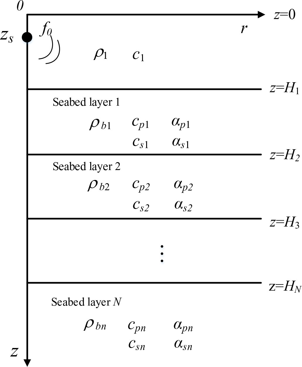
Figure 1 Shallow sea waveguide model with n-layered seabed.

In the model shown in Figure 1, under the wave theory, the wave equation can be transformed into a form that conforms to the Fourier transform through discrete processing. This enables the model to be solved quickly by the fast field method (FFM) (Zhu et al., 2012), and to derive the potential functions of each layer included in the wave equation. The relationship between the sound pressure p in the seabed layer and the potential function φ, represented by p=ρ₁ω²φ, is then used to obtain the value of the sound pressure at each point in the seabed layer. Where ω represents the angular frequency corresponding to the source frequency f, that is ω=2πf. The sound pressure field can be expressed as follows, where ξ represents the wave number.

$\begin{array}{ll}\mathit{p}\left(r,z,\omega \right)={\mathit{\rho }}_1{\omega }^2{\displaystyle {\int }_0^{\infty }{Z}_1\left(z,\xi ,\omega \right)}{J}_0\left(\xi r\right)\xi d\xi & (1)\end{array}$

The random variables d and m represent the experimental data from the sound field and the awaiting inversion geoacoustic parameters in the seabed model (Zhu et al., 2019). The vectors d and m satisfy the Bayesian theorem.

$\begin{array}{ll}\mathit{P}\left(\mathbf{m}|\mathbf{d}\right)=\mathit{P}\mathbf{\left(}\mathbf{d}|\mathbf{m}\right)\mathit{P}\left(\mathbf{m}\right)/\mathit{P}\left(\mathbf{d}\right)& (2)\end{array}$

where P(m|d) is the posterior probability density (PPD), P(d) is the probability density function (PDF) of d, P(m) is the prior PDF, and represents the available parameter information independent of the data. P(d|m) is the conditional PDF of m under the given measured data d, which is expressed by the likelihood function L(d|m) for the measured data. Thus, Equation (2) can be written as

$\begin{array}{ll}P\mathbf{\left(}\mathbf{m}|\mathbf{d}\right)\propto L\left(\mathbf{m}\right)P\left(\mathbf{m}\right)& (3)\end{array}$

The likelihood function is determined by the form of the measured data and the statistical distribution of the data errors. In practice, obtaining an independent estimate of the error statistics is often tricky; thus, the assumption of unbiased Gaussian errors is used in processing, and the likelihood function is given by

$\begin{array}{ll}L\left(\mathbf{m}\right)=P(\mathbf{d}|\mathbf{m})\propto \exp \left[-E\left(\mathbf{m}\right)\right]& (4)\end{array}$

where E(m) represents the error function. After normalization, we obtain

$\begin{array}{ll}P(\mathbf{m}|\mathbf{d})=\frac{\exp \left[-E\left(\mathbf{m}\right)\right]P(\mathbf{m})}{{\displaystyle \int \exp \left[-E\left(\mathbf{m}\text{'}\right)\right]P(\mathbf{m}\mathbf{\text{'}})\text{d}\mathbf{m}\mathbf{\text{'}}}}& (5)\end{array}$

The domain of integration spans the M-dimensional parameter space.

In the Bayesian inversion method, the multidimensional PPD of m represents the most general solution to the inversion problem. However, interpreting the PPD for a multi-dimensional problem requires the properties to be estimated by defining the parameter values, uncertainties, and inter-relationships, such as the MAP model, mean model, and marginal probability distributions, which are defined, respectively, as

$\begin{array}{ll}\widehat{\mathbf{m}}=A{\text{rg}}_{\max }\left\{P\left(\mathbf{m}|d\right)\right\}& (6)\end{array}$

$\begin{array}{ll}\overline{\mathbf{m}}={\displaystyle \int \mathbf{m}\mathbf{\text{'}}P(\mathbf{m}\mathbf{\text{'}})\text{d}\mathbf{m}\mathbf{\text{'}}}& (7)\end{array}$

$\begin{array}{ll}P({\mathbf{m}}_{\mathbf{i}}|\mathbf{d})={\displaystyle \int }\delta ({\mathbf{m}}_{\mathbf{i}}={\mathbf{m}}_{\mathbf{i}}^{\mathbf{\prime }})P({\mathbf{m}}^{\mathbf{\prime }}\mathbf{|}\mathbf{d})\text{d}{\mathbf{m}}^{\mathbf{\prime }}& (8)\end{array}$

where δ is the Dirac delta function, and the range of the integral is the space of each parameter.

Inter-parameter relationships are quantified by normalizing the covariance matrix C_m to produce a correlation matrix with elements between +1 and −1.

$\begin{array}{ll}{R}_{ij}=\frac{C_{m_{ij}}}{\sqrt{C_{m_{ii}}{C}_{m_{jj}}}}& (9)\end{array}$

where the parameters are completely positively correlated for R_ij= +1 and negatively correlated for R_ij = −1. Furthermore, R_ij = 0 indicates that the parameters were not relevant.

MAP estimates in this study were computed using the OSA. Marginal distributions were determined by numerical integration of the PPD, which was obtained using MHS. Although the MHS results do not depend on the initial model, the accuracy of the inversion results can be improved by selecting the correct initial value. In this study, the MAP estimate searched by the OSA was used as the initial model for the MHS (Zheng et al., 2020).

In Bayesian inversion theory, solving the PPD requires the likelihood function to be obtained. In addition, because the uncertainties in the data are often not well known, physically reasonable assumptions are required for the form of the uncertainty distribution; thus, assuming the data errors are independent Gaussian-distributed random variables, the likelihood function can be given by

$\begin{array}{ll}L\left(\mathbf{m}\right)={\displaystyle \prod _{f=1}^F\frac{1}{{\pi }^k\left|C_{\text{m}}^f\right|}}\exp \left\{-{\left[{\text{P}}_{mea}^f-{\text{P}}_{pre}^f\left(\mathbf{m}\right)\right]}^T{\left(C_{\text{m}}^f\right)}^{-1}\left[{\text{P}}_{mea}^f-{\text{P}}_{pre}^f\left(m\right)\right]\right\}& (10)\end{array}$

where ${\mathbf{\text{ p}}}_{\text{mea}}^{\mathbf{\text{f}}}(\mathbf{\text{m)}}$ represents the measured sound pressure data at K receiving positions for the f^th frequency, and ${\mathbf{\text{p}}}_{\text{pre}}^{\mathbf{\text{f}}}(\mathbf{\text{m)}}$ and ${\mathbf{\text{ C}}}_m^f$, respectively, represent the sound pressure data predicted by the model and the covariance matrix under the same conditions (Dong and Dosso, 2011; Gao et al., 2017).

The sound pressure predicted by the model, ${\text{p}}_{\text{pre}}^{\text{f}}(\mathbf{\text{m)}}$, can be expressed as

$\begin{array}{ll}{\mathbf{p}}_{\text{pre}}^{\mathbf{f}}\left(\mathbf{m}\right)=A^f{\text{e}}^{\text{i}{\theta }^f}{\mathbf{p}}_{\text{FFM}}^{\mathbf{f}}\left(\mathbf{m}\right)& (11)\end{array}$

where ${\mathbf{\text{p}}}_{\text{FFM}}^{\mathbf{\text{f}}}\mathbf{\text{(m)}}$ is the sound pressure computed by the FFM, and A^f and θ^f are the magnitude and phase of the unknown complex source at each frequency, respectively. Then, the likelihood can be maximized with respect to the source by setting ∂L(m)/∂A^f=∂L(m)/∂θ^f=0, leading to

$\begin{array}{ll}{A}^f{\text{e}}^{\text{i}{\theta }^f}=\frac{{\left[{\mathbf{p}}_{\text{FFM}}^f\left(\mathbf{m}\right)\right]}^{*}{\mathbf{p}}_{\text{mea}}^f}{{\left|{\mathbf{p}}_{\text{FFM}}^f\left(\mathbf{m}\right)\right|}^2}& (12)\end{array}$

where “*” denotes the conjugate transpose.

For each frequency, the standard approximation of the diagonal covariance ${\text{ C}}_m^f{\text{=v}}^{\text{f}}\text{I}$, where v^f is the unknown variance at the f^th frequency, and I is the identity matrix, in which case the likelihood function becomes

$\begin{array}{ll}L(\mathbf{m})=\prod _{f=1}^F\frac{1}{{(\pi v^f)}^K}\exp \left[-\frac{B^f(\mathbf{m}){\left|{\mathbf{p}}_{\text{mea}}^f\right|}^2}{v^f}\right]& (13)\end{array}$

where B^f(m) represents the normalized Bartlett disqualification, which can be expressed as

$\begin{array}{ll}{B}^f(\mathbf{m})=1-\frac{{\left|{\left[{\mathbf{p}}_{\text{FFM}}^f\left(\mathbf{m}\right)\right]}^{*}{\mathbf{p}}_{\text{mea}}^f\right|}^2}{{\left|{\mathbf{p}}_{\text{mea}}^f\right|}^2{\left|{\mathbf{p}}_{\text{FFM}}^f\left(\mathbf{m}\right)\right|}^2}& (14)\end{array}$

To obtain a maximum likelihood estimate of the data variance by setting ∂L(m)/∂v^f = 0, the maximum likelihood solution of the variance estimate can be expressed as

$\begin{array}{ll}{\widehat{v}}_f=\frac{B^f(\mathbf{m})\left|{\left|{\mathbf{p}}_{\text{mea}}^f\right|}^2\right|}{K}& (15)\end{array}$

Substituting Equation (15) into Equation (13) and Equation (4), the error function E(m) becomes

$\begin{array}{ll}E(\mathbf{m})=K{\displaystyle \sum _{f=1}^F\ln \left[B^f(\mathbf{m}){\left|{\mathbf{p}}_{\text{mea}}^f\right|}^2\right]}& (16)\end{array}$

Determining an appropriate model parameterization is another essential aspect of geoacoustic parameter inversion. Model selection involves selecting a set of parameterized models that are most consistent with the measured data based on a certain target criterion. Models for which either too many or too few parameters are specified (over-parameterization and under-parameterization, respectively) are known to have a certain impact on the inversion results (Dettmer et al., 2009; Li et al., 2012). In this study, BIC is used to select the parameterized model that is most consistent with the measured data. BIC is an asymptotic approximation of the Bayesian theorem P(d|I) of model I, and I denotes the presupposition of different inversion models. Assuming the measurement data d, the likelihood function of model I is expressed as follows

$\begin{array}{ll}-2\text{In}P(\mathbf{d}|\text{I})\approx \text{BIC = }-2\text{In}L(\widehat{\mathbf{m}})+M\text{In}N& (17)\end{array}$

The likelihood function is replaced with the error function to obtain, where M represents the number of model parameters, N represents the number of data

$\begin{array}{ll}\text{BIC = }2E(\widehat{\mathbf{m}})+M\text{In}N& (18)\end{array}$

The parameterization with the smallest BIC value was selected as the most appropriate model. According to Equation (18), the BIC value is determined by the error function, number of parameters, and number of measured data points. Therefore, minimizing the BIC provides a balance between the error value and number of parameters, identifying the simplest parameterization consistent with the resolving power of the data.

2.2 Optimised simulated annealing

Searching for the MAP values in the prior interval based on the error function is an important step in the Bayesian inversion method. Because the error function is nonlinear, multi-dimensional, and may have multiple peaks, the search process is highly challenging, and the correlation between the parameters complicates the search. Currently, most researchers apply global optimization algorithms, such as SA and GA, to search for the MAP (Dosso et al., 2001). In geoacoustic parameter inversion for a multi-layer seabed, the number of awaiting inversion parameters increases as the number of layers in the seabed increases, and the choice of the parameter prior interval also becomes more difficult. An interval range that is too large increases the difficulty, at the same time, reduces the accuracy of the results, whereas a range that is too small may not include the true value of the geoacoustic parameters in the interval. The use of traditional global optimization algorithms, owing to the lack of effective limiting measures, usually involves setting large prior intervals for the inversion, resulting in low inversion efficiency and poor results. The effective reduction of the range of the previous interval in the optimization process would enable the accuracy and efficiency of the inversion result to be effectively improved (Ohta et al., 2008).

Previous research showed that the solution to multi-layer sea environment problems led to the emergence of an objective law according to which the value of the acoustic impedance in the seabed generally increases with the depth of the seabed (Yang, 2009; Li, 2012). This law provides the possibility of narrowing the prior interval in the inversion. Therefore, the OSA we proposed is based on the SA algorithm, which is an improved SA that can be used to correct the prior interval in the process of optimizing and solving the parameters according to the acoustic impedance law of the upper and lower layers of the seabed (Xue et al., 2021). The algorithm first optimizes and solves the parameters of the lower layer, and adds constraints on the basis of the existing results to realize the accurate solution of the parameters of the upper layer. The inversion flow chart that includes the additional correction process is shown in Figure 2.

FIGURE 2

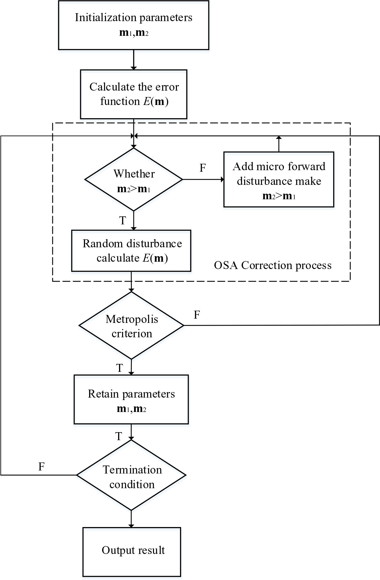
Figure 2 Inversion flow chart reflecting the additional correction process.

3 Simulation analysis

Selecting an appropriate forward model is crucial for improving the accuracy of the inversion (Seongryong et al., 2016; Enming et al., 2018). For shallow sea environments, the seabed is regarded as a uniform and isotropic multi-layer medium, and the density ρ_b, compression wave speed c_p, shear wave speed c_s, and the two types of wave speed attenuation α_p and α_s are taken as the inversion objects in this study. To verify the reliability of the above-mentioned theoretical research pertaining to inversion, a simulation example was used for verification. In this example, the seabed is modelled as a two-layer elastic medium. The true values are listed in Table 1, where the source frequency is 155 Hz, the depth of the sound source z_s is 20 m, the receiving depth z_r is 10 m, and the depth of the sea H₁ is 100 m. The transmission loss (TL) is calculated by FFM under the true value condition (Zhu et al., 2012), as shown in Figure 3. The sound waves propagating in the sound field can be regarded as the superposition of normal waves of different orders. The superposition of normal waves is related to the phase and will show interference structure. Thus, the TL at different locations is up and down, and the TL increases significantly at the 500m location due to the reverse superposition of a large number of normal positive waves.

TABLE 1

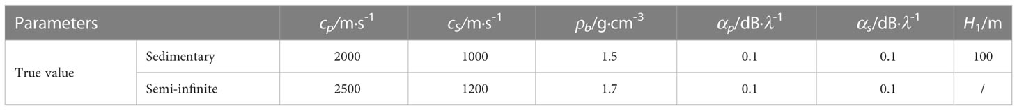
Table 1 Parameters used for the simulation of the sea environment.

FIGURE 3

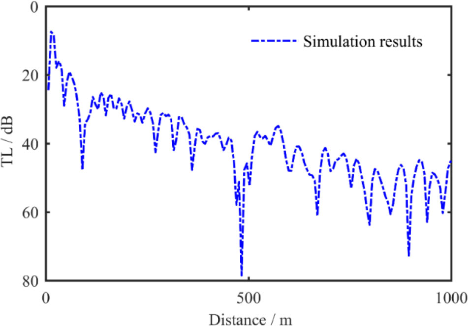
Figure 3 TL obtained by using the true value set in the simulation.

3.1 Model selection

The main discussion in this section is the feasibility of BIC. The sound pressure data obtained from the 2-layer model simulation is used as the validation object. Different inversion models are used to invert this set of sound pressures, When the BIC value is smallest, if the inversion results of the corresponding model best match. We considered three different versions of the inversion model: a parameterization model with one to three layers of the isotropic uniformly distributed seabed. Based on the sound pressure values obtained under the simulation conditions listed in Table 1, we used the OSA to get the BIC values corresponding to the inversion results for the different versions of the model for model selection.

The results of the study designed to select the model were obtained from the simulation analysis and are shown in Figure 4. Here, m₁, m₂, and m₃ represent the inversion model of the one-, two-, and three-layer uniformly distributed seabed, respectively. Figure 4A shows that the simulation inversion of different models lowers the error value as the number of layers in the model increases, with the error value of the one-layered model being the largest. Figure 4B shows that the number of parameters that need to be also considered increases, which increases the uncertainty of the inversion results. BIC fully considers the balance among the error values of the model, the number of parameters, and the number of data points and selects the parameterized model most consistent with the measured data. Figure 4C shows that the model based on the initial settings determined by BIC with the best fit is the two-layer model of the uniformly distributed seabed. These results show that the BIC can be employed to select the layered model of the seabed that best fits the parameters that were initially specified.

FIGURE 4

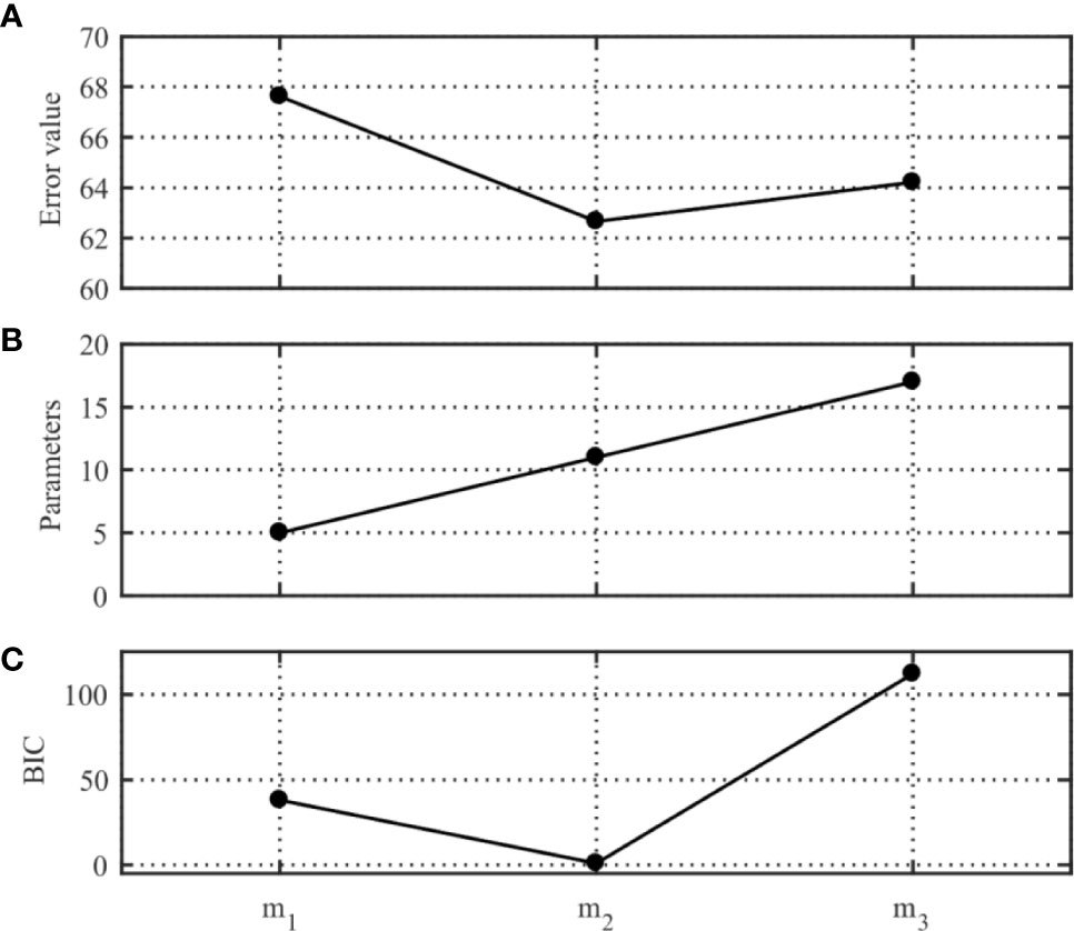
Figure 4 Results of the model selection study in terms of the (A) error value, (B) parameters, and (C) BIC, where m₁, m₂, and m₃ represent the inversion model of the one-, two-, and three-layer uniformly distributed seabed, respectively.

The TL values obtained by the different inversion models are compared in Figure 5. Figures 5A–C Shows the TL comparison between the inversion model using different layered structures and the two-layer structure simulation data inversion results. The results qualitatively indicate that the inversion model of the two-layer structure is the most consistent with the initially specified model and demonstrates that BIC can select the model with the best parameterization.

FIGURE 5

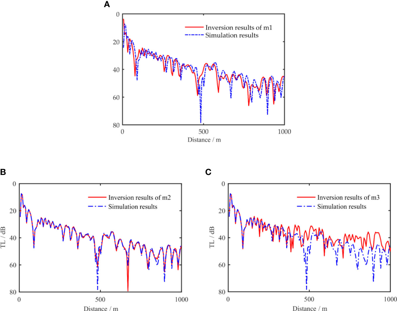
Figure 5 Comparison of transmission loss obtained by the different inversion models (A) m1, (B) m2, (C) m3. Inversion results of the simulation data of the two-layer structure using different layered structure inversion models. The blue dotted line indicates the transmission loss resulting from simulation with the true value set.

3.2 Optimisation error value by OSA

Many optimization algorithms, such as SA and GA, can optimize the error function (Bevans and Buckingham, 2016; Yang et al., 2017; Fu et al., 2018). However, application of the traditional optimization algorithm to the error function established in this study for the multi-layer uniformly layered seabed model often produces optimization results that do not conform to the actual physical laws. In addition, considering seabed stratification, the prior interval inevitably needs to be expanded. This means that the accuracy of the results obtained when the traditional optimization algorithm is optimized for the above model is greatly reduced. Because the conventional global optimization algorithms SA and GA have certain difficulties with the application of multi-layer seabed inversion, we proposed an improved algorithm (Julien et al., 2018; Li et al., 2018).

Table 2 compares the mean values and standard deviation (std) before and after the application of OSA. The results in the table indicate that the mean value of the optimization result after the application of OSA is closer to the true value obtained in the simulation, and the corresponding standard deviation is reduced; in particular, the parameters of the second seabed improved significantly. Figures 6, 7 show the PPD of the parameters of the first and second layers of the seabed, respectively. The red line represents the true value, and the blue line represents the distribution of the difference between the mean and standard deviation of the data results in the interval. These results show that the PPD distribution of the parameter inversion obtained after applying OSA is narrower. Figure 7 shows that the PPD distribution after application of the OSA is further concentrated near the true value; in particular, the improvement in the speed and density of the acoustic wave of the second seabed is more pronounced.

TABLE 2

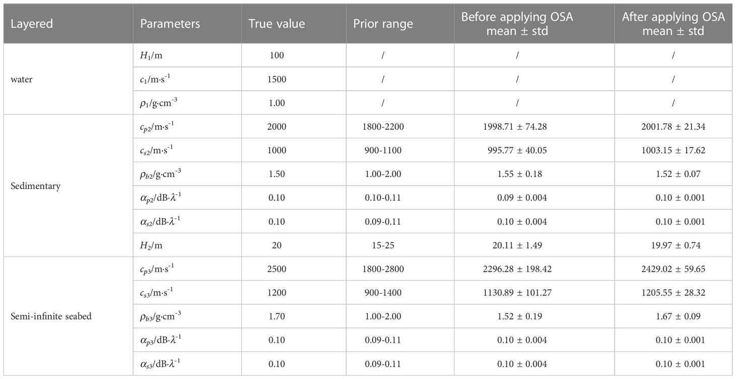
Table 2 Comparison of the mean and standard deviation of inversion parameters before and after improvement of the simulated algorithm.

FIGURE 6

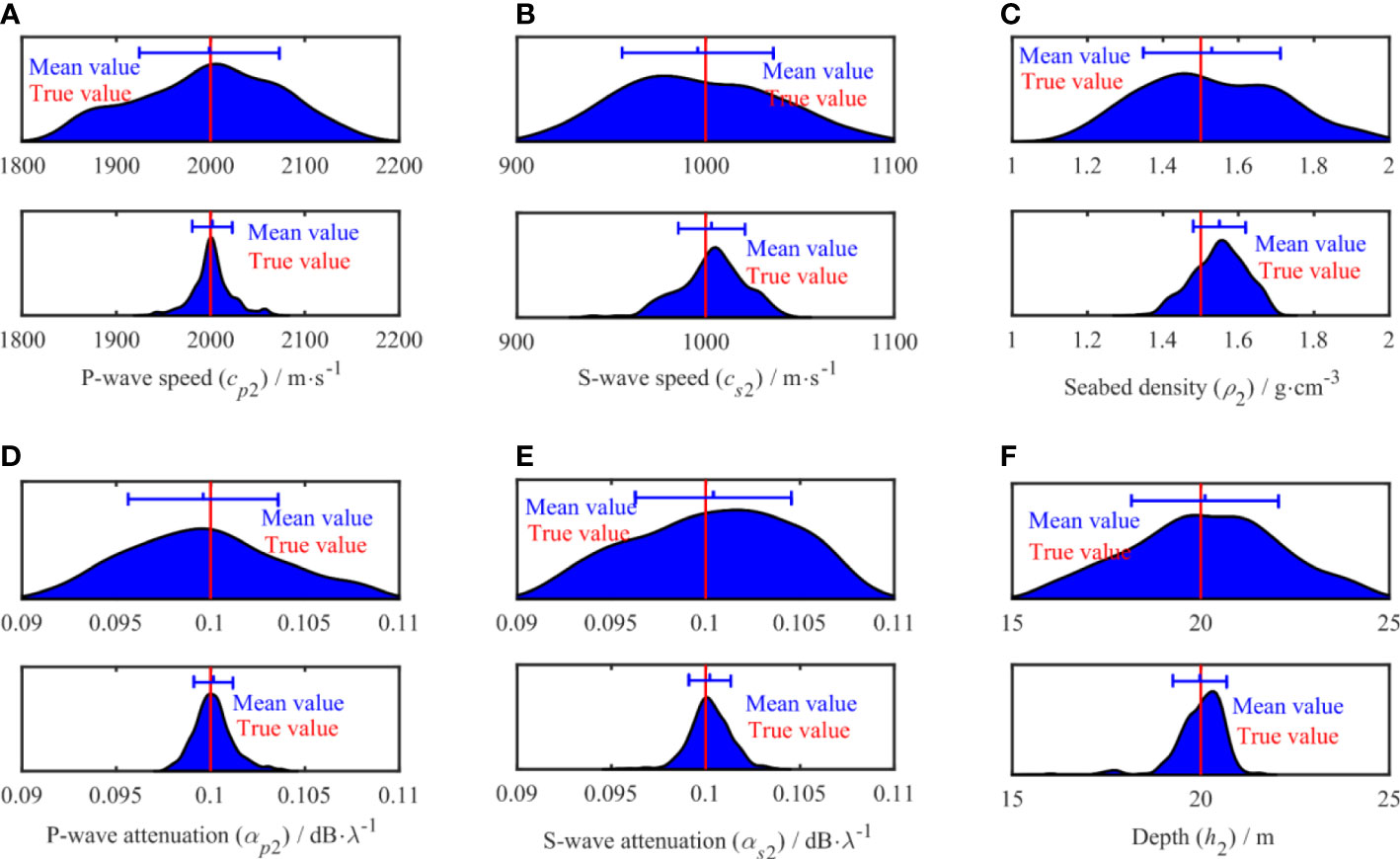
Figure 6 One-dimensional marginal probability distribution of sedimentary parameters.

FIGURE 7

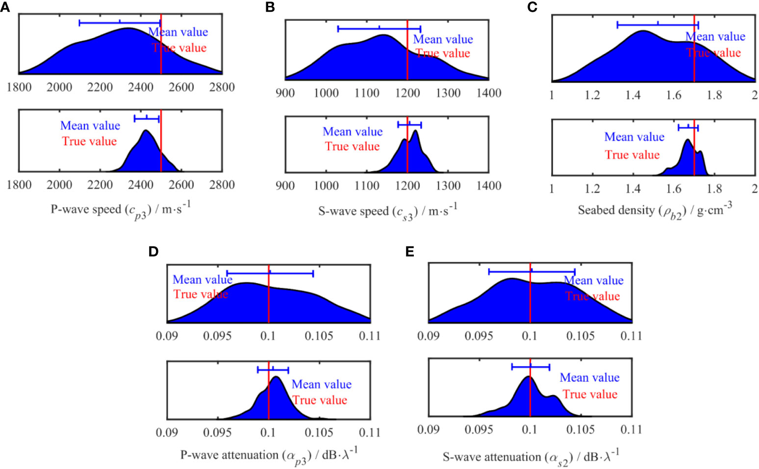
Figure 7 One-dimensional marginal probability distribution of semi-infinite parameters.

Figure 8 compares the sound pressure TL curve calculated by the average value of the inversion results of each parameter before and after the algorithm was improved with the TL curve calculated using the true value. This comparison reveals that the TL curve obtained by the improved optimization algorithm is in closer agreement with the TL curve obtained with the true value, which further demonstrates the feasibility of the improved algorithm. From the interpretation of the interference phenomenon, using the normal wave theory, it can be known that the rapid increase in TL here is caused by the interference and superposition of different order normal waves at this position, and the appearance of the interference structure makes the sound field more complicated.

FIGURE 8

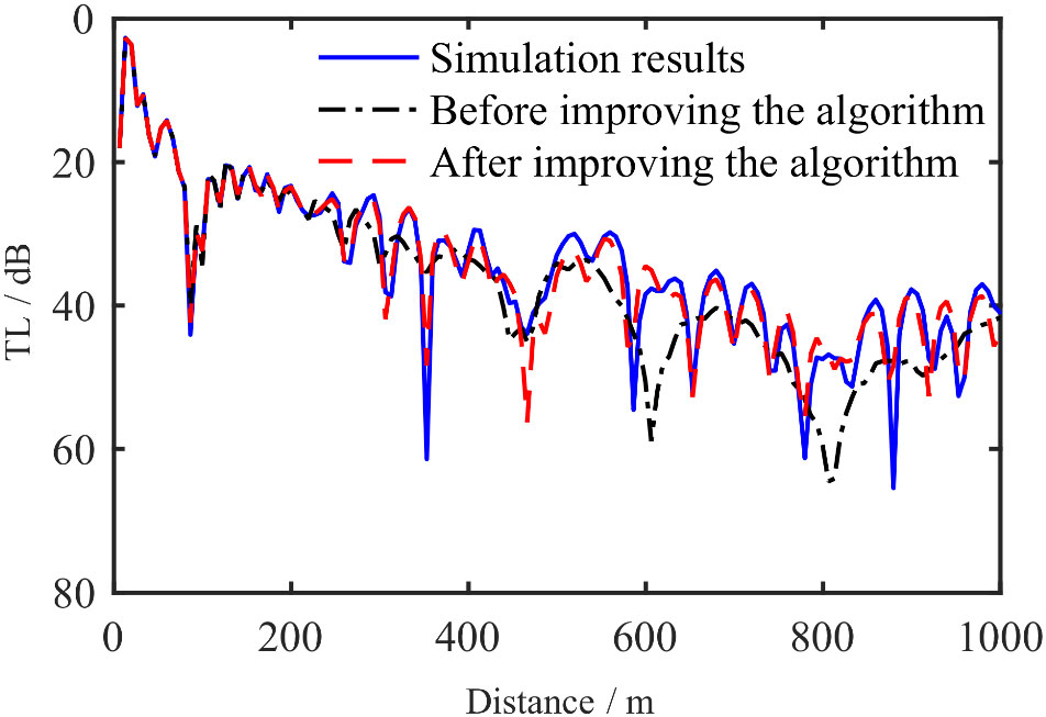
Figure 8 Comparison of transmission loss of inversion parameters before and after improvement of the algorithm.

4 Measurements and results

4.1 Introduction to the experiment

The propagation characteristics of high-frequency underwater acoustic signals in small-scale environments can be used to simulate the propagation characteristics of low-frequency signals in actual large-scale sea environments (Zhang et al., 2018; Zhang et al., 2022). Compared with the original sound field, the expression of the sound field calculated by the reduced-scale experiment is only increased in equal proportion, and the characteristics of the undulation and distribution of the sound pressure field remain the same. Detailed introduction to this topic can be found elsewhere (Zhu, 2014; Zheng et al., 2019).

The accuracy of the inversion method was verified by conducting a scaling experiment. The experiment was carried out in an anechoic tank in the laboratory using polyvinyl chloride (PVC) slab (size: 153 mm × 110 mm × 10.5 mm) to simulate the elastic semi-infinite seabed. A layer of fine sand was placed on the PVC slab to simulate a shallow sea waveguide environment with elastic sediment and an elastic semi-infinite seabed with a sand thickness of 250 mm. The experimental setup is shown in Figure 9, where the sound source sensor frequency is 155 kHz, the depth of the sound source sensors z_s is 200 mm, the receiving depth z_r is 200 mm, and the depth of the freshwater z₁ is 300 mm. The acoustic speed of the sound wave in the sea, calculated at room temperature (11.15°C) in the laboratory, was 1450.212 m·s^-1. A high-frequency underwater acoustic wave was transmitted by a source (a custom-built transmitting transducer), which was installed at a fixed position at one end of the equipment. The sound wave was received by a single acoustic sensor (a standard TC4038 underwater sensor), which was attached to the mobile micro-worktable to enable the position of the sensor to be varied at equal distances. This arrangement allowed the underwater sensor to move 2 mm every time, with an error of less than 20 µm. The movement of the mobile workbench was computer-controlled for data measurement and collection. Upon completion of the measurement in one position, the worktable automatically moved to the next position, and the measurement at each position was recorded ten times to obtain the average value for each position. A total of 500 locations were selected for measurement during the experiment (Ballard et al., 2009; Zheng, 2019).

FIGURE 9

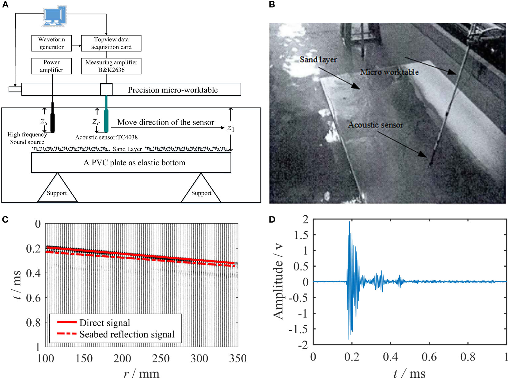
Figure 9 Experimental setup with the measuring instruments and equipment and time domain waveform. (A) Diagram of the layout of the experimental measurement system, (B) Photographic image of the movable micro-worktable for the measurement equipment, (C) Time domain waveform arrival time, (D) Time domain waveform at position 50.

Figure 9C gives the arrival times of the 50-150 channel time domain waveforms measured by the above experimental equipment, from which the direct and reflected waves can be observed more clearly. Figure 9D shows the time domain waveform of the signal received by the hydrophone at the 50th position. Since the experiments were conducted in an anechoic environment and the noise effect is relatively small, the arrival time of the signal in the time domain waveform can be used to distinguish between direct and reflected waves. We choose the bottom reflected wave as the actual signal used in the inversion.

4.2 Model selection

The feasibility of BIC has been verified in the simulation, and this section uses the BIC criterion to select the best parameterized model for the experimental data. Three models with different hierarchical structures are still applied to invert the experimental data, and the BIC values can be calculated by combining the error values and the number of model parameters obtained during the inversion of the different models. The BIC values are solved by Equation (17), the model with the smallest BIC value is the best parameterized model.

The results of the model selection are shown in Figure 10. Figure 10A shows that the error decreases substantially when proceeding from one to two seabed layers and that this reduction is significantly less when the number of layers is increased from two to three. Figure 10B shows that the number of parameters to be considered also increases, which raises the uncertainty of the inversion results. According to Figure 10C, the optimal model determined by BIC is a two-layer uniformly distributed seabed model.

FIGURE 10

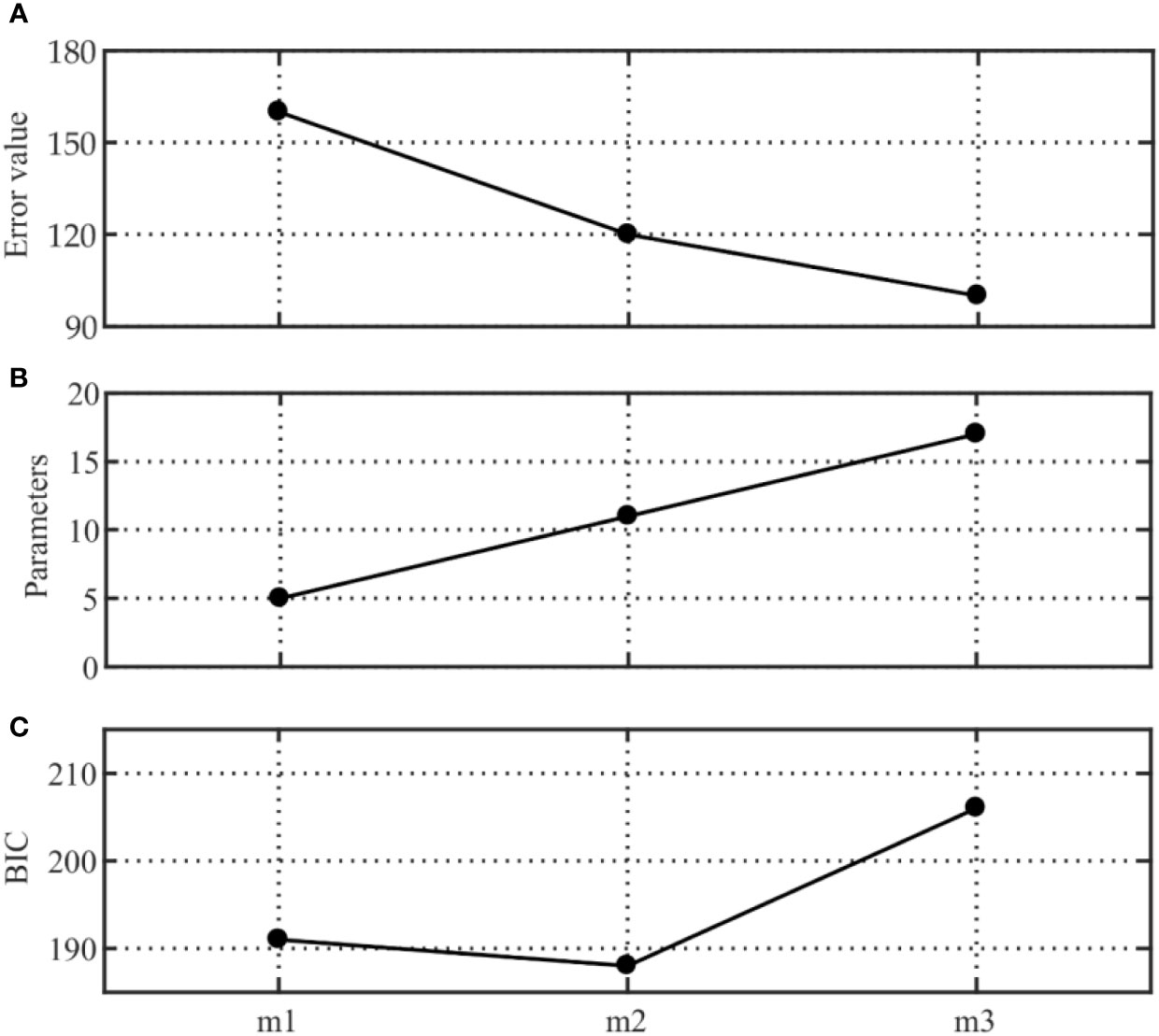
Figure 10 Results of the model selection study: (A) Error value, (B) parameters, and (C) BIC, where m₁, m₂, and m₃ represent the inversion model of the one-, two-, and three-layer uniformly distributed seabed, respectively.

Figure 11 shows the profile structure of the compression wave speed, shear wave speed, and variation in density with depth. The acoustic impedance at the bottom is proportional to the deep; that is, in general marine environment, the acoustic impedance increases with depth. The results indicate that the trends observed for the three different inversion models are consistent with this physical law. Moreover, increasing the stratification of the seabed does not include the “ reversal “ phenomenon in the distribution of parameters; this demonstrates the significance of OSA in searching for parameters in the prior interval. The structure of the section, with 1000 mm as the boundary, reveals an obvious structural division of the density, compression wave speed, and shear wave speed within this value. As the depth increased, each parameter tended to a certain value, and the change in the compression wave was particularly obvious.

FIGURE 11

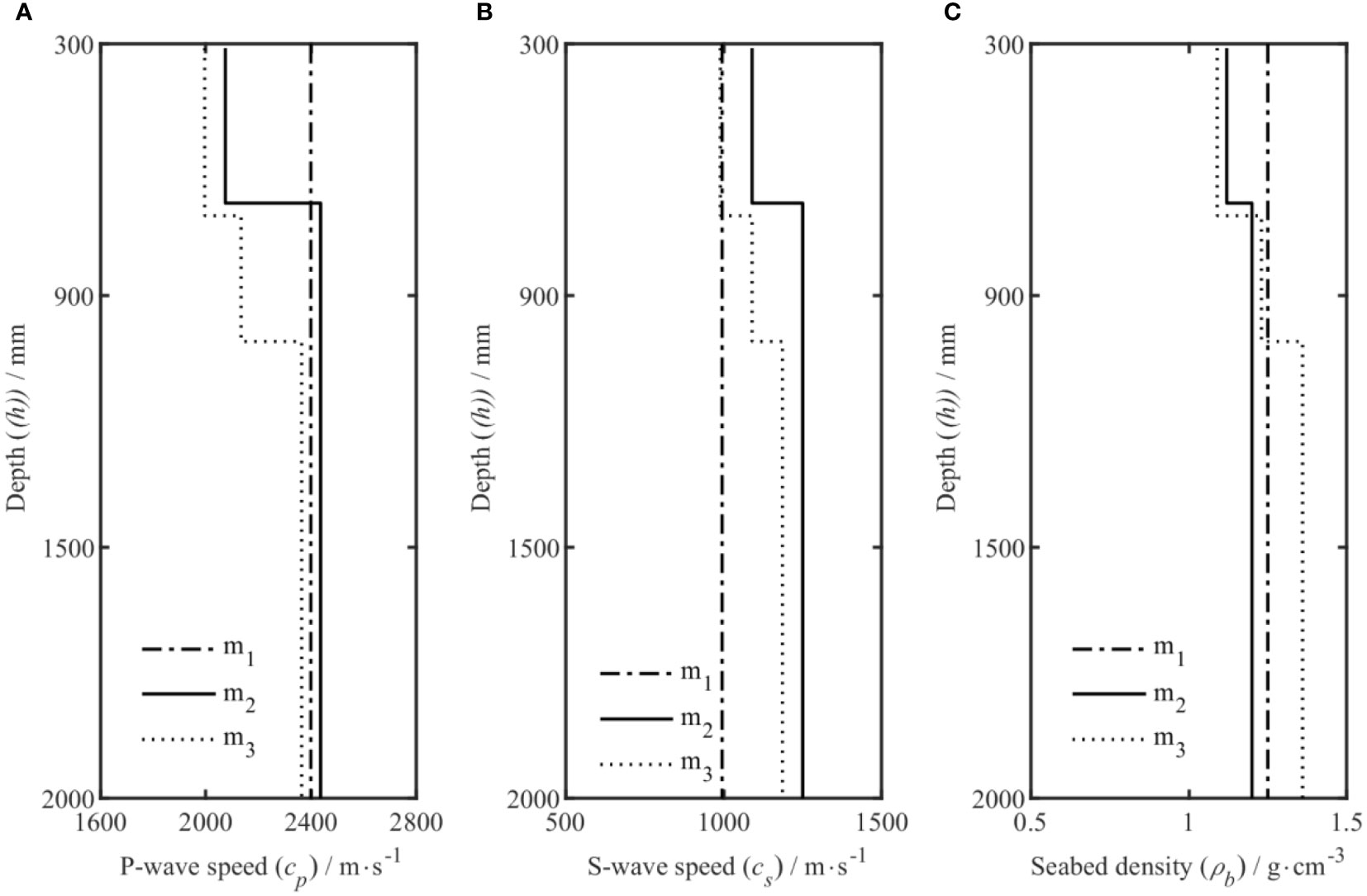
Figure 11 Density, compression wave speed, and shear wave speed profiles from the model selection study, where m₁, m₂, and m₃ represent the inversion model of the 1-layer, 2-layer, and 3-layer uniformly distributed seabed, respectively. (A–C) Relationship of c_p, c_s, and ρ with depth, respectively.

4.3 Inversion results and uncertainty analysis

The BIC optimization results demonstrate that the two-layer uniformly layered seabed model is the most consistent with the experimental results. The inversion results of this model are therefore analyzed and discussed in this section. Figure 12 compares the TL between the inversion data of the MAP model and the data acquired by conducting experimental measurements, the TL obtained by inversion uses the same source frequency as the experimental data. Figure 12 shows that Comparison of the transmission loss between the measured data and the inversion data, Table 3 lists the prior inversion intervals and the mean of the inversion results. The density of the polyvinyl chloride (PVC) slab that was used to simulate the semi-infinite seabed is known to be 1.20 g·cm^-3, and the thickness of the sediment, simulated by sand in our experiments, is approximately 250 mm. The average density of the semi-infinite seabed obtained by inversion was 1.21 g·cm^-3, and the average thickness of the sedimentary layer was 249.69 mm. The results show that the inversion results were consistent with the experimental results.

FIGURE 12

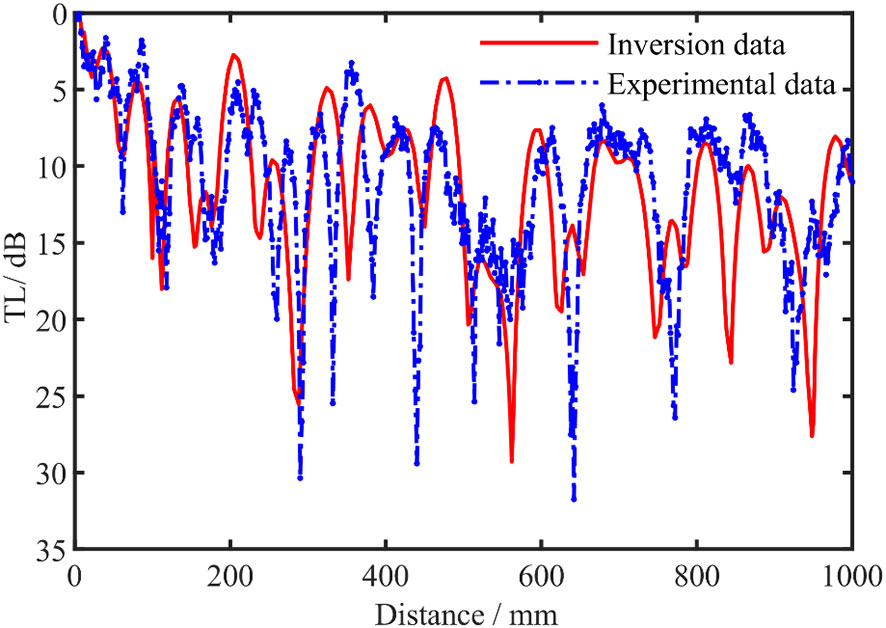
Figure 12 Comparison of the transmission loss between the measured (dashed blue trace) and the inversion data (solid red trace).

TABLE 3

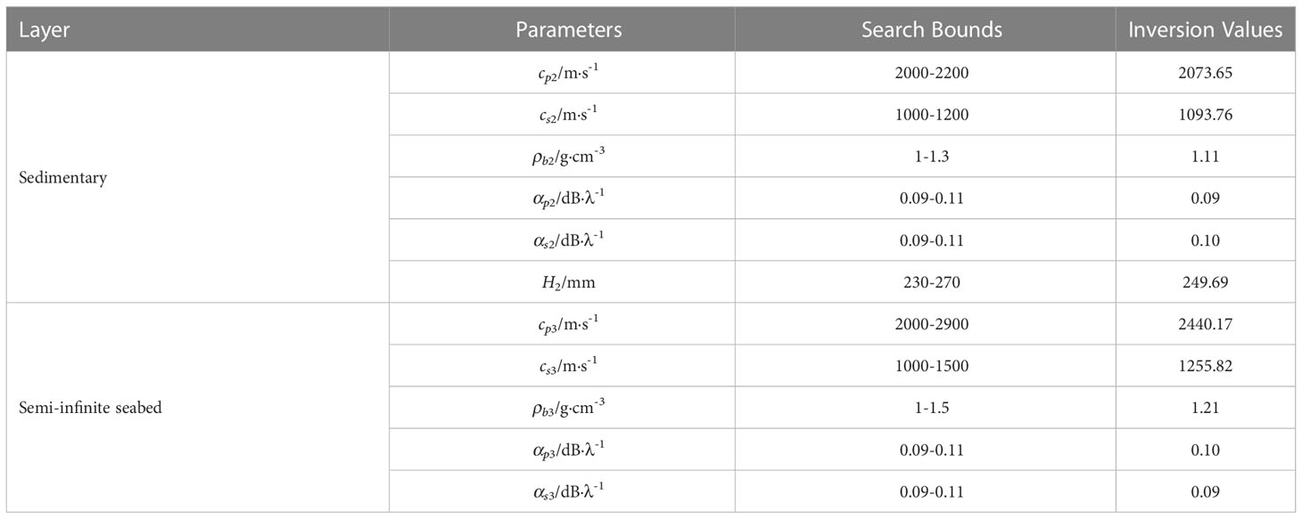
Table 3 Results of the measured inversion data.

In addition, we compared the inversion results with those obtained in the simulation of a semi-infinite seabed with a plate of the same material. The inversion results showed that the speed of the compression wave and the shear wave was 2399.36 m·s^-1 and 1242.97 m·s^-1, respectively. Considering that the sediment layer was replaced by fine sand and that there were many uncertain factors, such as the uniformity of the fine sand, errors would inevitably exist. Thus, the inversion results obtained for the speed of the compression wave and the shear wave of the semi-infinite seabed in this study were basically the same. It further verified the correctness of the inversion method proposed in this paper.

The uncertainty analysis of each parameter obtained by the inversion is helpful to judge the difficulty of accurate inversion of each parameter. The estimated value obtained by the OSA method was used as the initial model for sampling, and the PPD numerical integration solution of the parameters was obtained using the MHS method. The one-dimensional probability distribution map of the parameters corresponding to the two-layer uniform seabed distribution model is shown in Figures 13, 14, where the red solid line represents the MAP value of each parameter, and the blue line represents the distribution of the difference between the mean and standard deviation of the data result in the interval. In the figure, the one-dimensional marginal probability distribution of the parameters in the sedimentary layer and the semi-infinite seabed follows a normal distribution in the prior interval. The distribution of the sedimentary parameters is narrower than that of the semi-infinite seabed, indicating that these parameters are more sensitive. From the point of view of a single parameter, the distributions of c_p2, c_s2, and c_s3 are narrow. This shows that the parameter can be well distinguished, and the uncertainty is small; in contrast, c_p3 and the results of the wave speed attenuation distribution in each layer are poor, indicating that the uncertainty of this parameter is relatively large and that the parameter is not easy to determine.

FIGURE 13

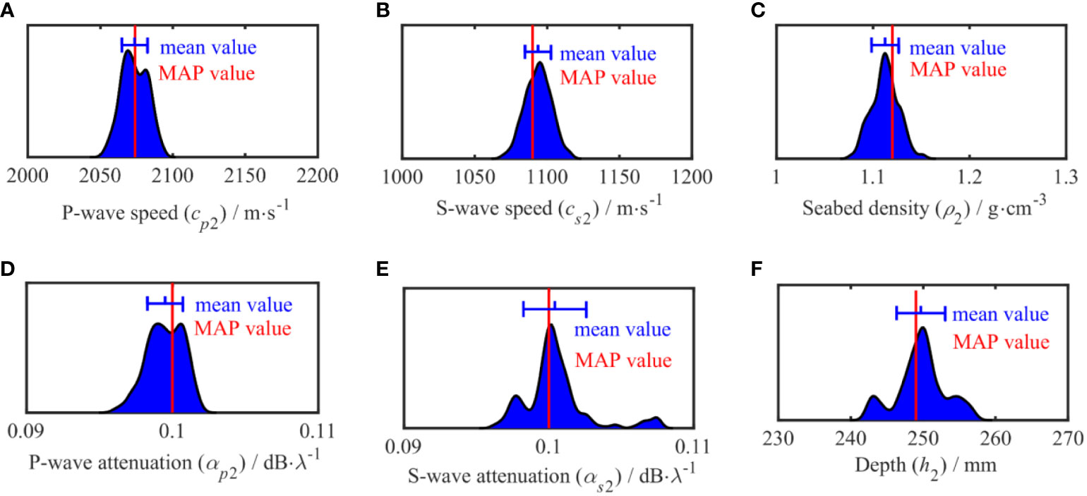
Figure 13 One-dimensional marginal probability distribution of sedimentary parameters.

FIGURE 14

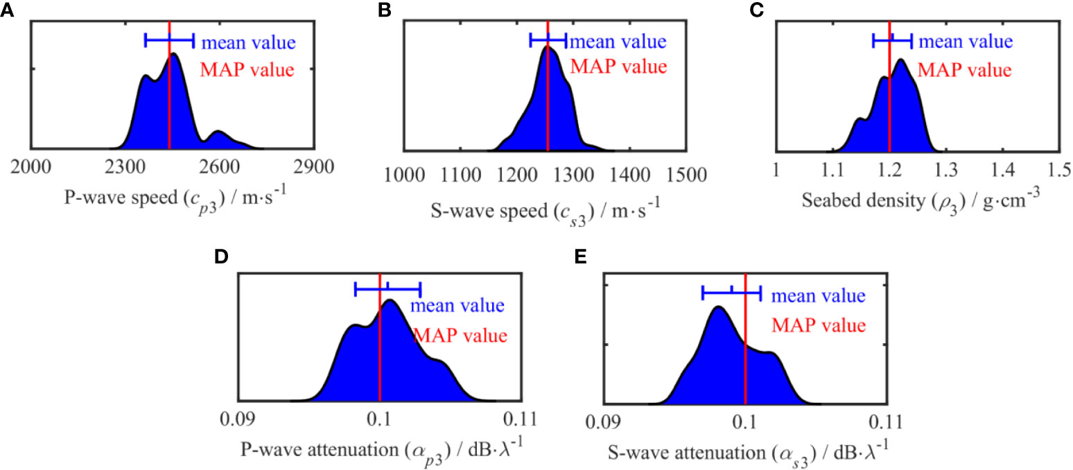
Figure 14 One-dimensional marginal probability distribution of semi-infinite parameters.

The inversion of the geoacoustic parameters is a multi-parameter optimization problem; the parameters are coupled with each other, and the correlation between the parameters directly affects the inversion results and increases the uncertainty in the parameters that need to undergo inversion. Therefore, we considered it necessary to analyze the extent to which the inversion parameters are correlated. The parameter correlation matrix (Figure 15) shows a strong positive correlation between α_s2 and c_p3. In addition, c_s3 and α_p3 are also strongly positively correlated, and this also holds for c_p2 and ρ_b2. In contrast, α_s2 and ρ_b2 have a negative correlation, and a strong negative correlation exists between h₂ and ρ_b2 and ρ_b3.

FIGURE 15

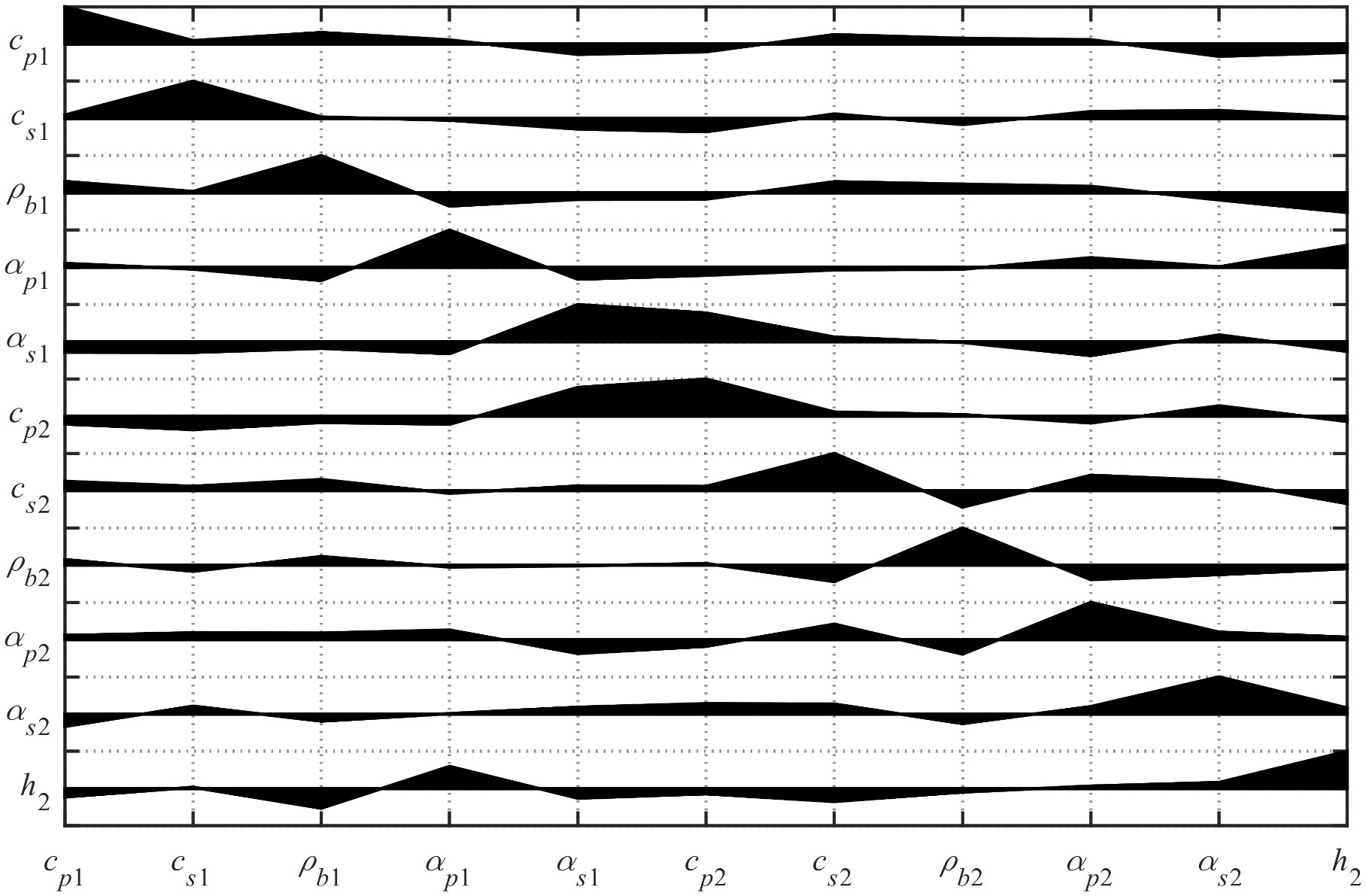
Figure 15 Correlation matrix diagram between inversion parameters.

Figure 11 shows the profile structure of parameters, which is intended to represent the depth distribution of parameters corresponding to the MAP, in which each parameter is a specific value. However, what we want to show in Figure 16 is the two-dimensional edge probability density distribution of parameters changing with depth, highlighting that the two-dimensional edge probability density of different layers and parameters is different, while the distribution range of color represents the probability density distribution, that is, the uncertainty of parameters. Figures 16A–C shows the two-dimensional edge probability distribution of the compression wave speed, shear wave speed, and density with depth to express the relationship among these parameters more intuitively and accurately. Because the inversion parameters are related to those of the sedimentary layer and lower seabed, the two-dimensional edge probability density distribution starts from the sedimentary layer. The results showed that, compared with the semi-infinite seabed, the probability distribution of the compression wave speed, shear wave speed, and density of the sedimentary layer were narrower and less uncertain, which further indicated that the parameters of the sedimentary layer were more sensitive.

FIGURE 16

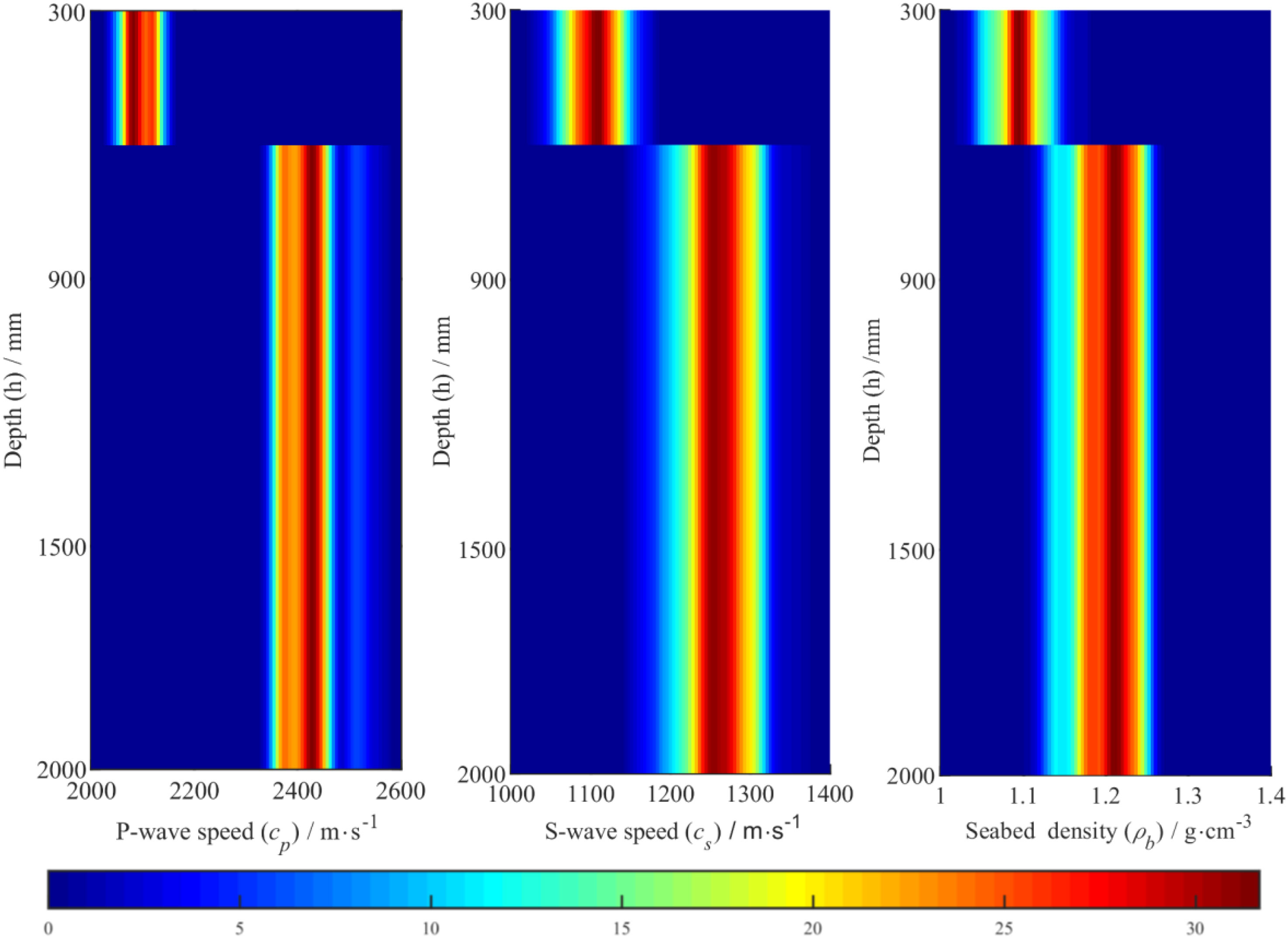
Figure 16 Two-dimensional marginal probability distribution. (A-C) two-dimensional edge probability distribution of compression wave speed, shear wave speed and density with depth.

5 Conclusions

The nonlinear Bayesian inversion method is not only valuable for effectively estimate the MAP model of the seabed parameters and analyzing the uncertainty in these parameters from a statistical point of view. In this study, our method based on nonlinear Bayesian inversion theory was employed for the inversion of geoacoustic parameters, which enriches and improves the related fields of geophysics and sea acoustics. Furthermore, the proposed method has essential prospects for practical application to seabed resource exploration, sea environment detection, sea engineering, and sea development. Specifically, in this study, a nonlinear Bayesian inversion method was used to invert the pressure field created by underwater sound wave as detected by underwater sensors. We varied the number of layers in the seabed in the parameterized models that we considered. Then, the optimal model was selected using the BIC, and the uncertainty in the inversion results was analyzed. The following conclusions were drawn:

(1) Bayesian inversion of the pressure field of sound can be used to obtain the parameters that define the seabed. The optimal model determined by BIC is a two-layer uniform seabed distribution model, which is consistent with the experimental results, The TL comparison results also prove the feasibility of the inversion method.

(2) With the aim of developing a nonlinear Bayesian inversion method based on the multi-layer seabed model, in the context of the research discussed in this article, the OSA was able to compute the estimated value of MAP efficiently and accurately, and avoided the phenomenon of parameter “reversal” in the multi-layer seabed model. OSA can improve the accuracy of the inversion results, which is verified in the simulation.

(3) The uncertainty analysis of the inversion results enabled us to conclude that, compared with the compression wave speed attenuation, shear wave speed attenuation, and density, the uncertainty in the compression wave speed and shear wave speed is smaller when the inversion of the sound pressure field is used for the calculation, and these parameters have greater sensitivity. Compared with those in the case of semi-infinite seabed, the sediment layer parameters are more sensitive and less uncertain.

Data availability statement

The original contributions presented in the study are included in the article/supplementary material. Further inquiries can be directed to the corresponding author.

Author contributions

YX processed data, reviewed literature and wrote the original manuscript. HZ co-authored the “Abstract,” “Introduction,” and supervised the study and reviewed the manuscript. XW contributed to data. GZ provides support in optimization algorithm. XL and JW contributed to image format modification. All authors contributed to the article and approved the submitted version.

Funding

This research was found by the National Natural Science Foundation of China (Grant No: 11704337), the Stable Supporting Fund of Acoustic Science and Technology Laboratory (Grant No: JCKYS2020604SSJS011), the Open Foundation from Marine Sciences in the First-Class Subjects of Zhejiang (20200101) and the Youth Innovation Promotion Association CAS (Grant No. 2020023). The Science Foundation of Donghai Laboratory (Grant No: DH-2022KF01018).

Acknowledgments

We acknowledge the National Key Laboratory, College of Underwater Acoustic Engineering, Harbin Engineering University, China for supporting in this research.

Conflict of interest

The authors declare that the research was conducted in the absence of any commercial or financial relationships that could be construed as a potential conflict of interest.

Publisher’s note

All claims expressed in this article are solely those of the authors and do not necessarily represent those of their affiliated organizations, or those of the publisher, the editors and the reviewers. Any product that may be evaluated in this article, or claim that may be made by its manufacturer, is not guaranteed or endorsed by the publisher.

References

Ballard M.-S., Becker K.-M., Goff J.-A. (2009). Geoacoustic inversion for the new Jersey shelf: 3-d sediment model. IEEE J. Oceanic. Eng. 35, 28–42. doi: 10.1109/JOE.2009.2034490

CrossRef Full Text | Google Scholar

Benavente R., Dittmer J., Cummins P.-R., Sambridge M. (2019). Efficient Bayesian uncertainty estimation in linear finite fault inversion with positivity constraints by employing a log-normal prior. Geophys. J. Int. 217, 469–484. doi: 10.1093/gji/ggz044

CrossRef Full Text | Google Scholar

Bevans D.-A., Buckingham M.-J. (2016). A geoacoustic inversion technique using the low-frequency sound from the main rotor of a Robinson R44 helicopter. J. Acoust. Soc Am. 140, 3169–3169. doi: 10.1121/1.4969952

CrossRef Full Text | Google Scholar

Dettmer J., Dosso S.-E., Holland C.-W. (2009). Model selection and Bayesian inference for high-resolution seabed reflection inversion. J. Acoust. Soc Am. 125, 706–716. doi: 10.1121/1.3056553

PubMed Abstract | CrossRef Full Text | Google Scholar

Dong H.-F., Dosso S.-E. (2011). Bayesian Inversion of interface-wave dispersion for seabed shear-wave acoustic profiles. IEEE J. Oceanic. Eng. 36, 1–11. doi: 10.1109/JOE.2010.2100490

CrossRef Full Text | Google Scholar

Dosso S.-E., Dettmer J. (2011). Bayesian Matched-field geoacoustic inversion. Inverse. Problems. 27, 55009. doi: 10.1088/0266-5611/27/5/055009/meta

CrossRef Full Text | Google Scholar

Dosso S.-E., Nielsen P.-L., Harrison C.-H. (2009). Bayesian Inversion of reverberation and propagation data for geoacoustic and scattering parameters. J. Acoust. Soc Am. 125, 2867. doi: 10.1121/1.3106524

PubMed Abstract | CrossRef Full Text | Google Scholar

Dosso S.-E., Wilmut M.-J., Lapinski A.-L. S. (2001). An adaptive-hybrid algorithm for geoacoustic inversion. IEEE J. Oceanic. Eng. 26, 324–336. doi: 10.1109/48.946507

CrossRef Full Text | Google Scholar

Enming X., Rongwen G., Dosso S.-E., Jianxin L., Hao D. (2018). Efficient hierarchical trans-dimensional Bayesian inversion of magnetotelluricdata. Geophys. J. Int. 213, 1751–1767. doi: 10.1093/gji/ggy071

CrossRef Full Text | Google Scholar

Fu D., Xiao G., Zhou L. (2018). Nonlinear Bayesian theory and BIC criterion-based on high precision Rayleigh wave inversion of cutoff-wall. Water Resour. Hydropower. Eng. 49, 64–70. doi: 10.13928/j.cnki.wrahe.2018.08.008

CrossRef Full Text | Google Scholar

Gao F., Pan C., Sun L. (2017). Geoacoustic parameters inversion of bayes matched-field: A multi-annealing Gibbs sampling algorithm. Acta Armamentarii. 38, 1385–1394. doi: 10.3969/j.issn.1000-1093.2017.07.017

CrossRef Full Text | Google Scholar

Julien B., Ying T.-L., Dimitrios E., Goff J.-A., Dosso S.-E. (2018). Geoacoustic inversion on the new England mud patch using warping and dispersion curves of high-order modes. J. Acoust. Soc Am. 143, 405–411. doi: 10.1121/1.5039769

CrossRef Full Text | Google Scholar

Li C. (2012). Study of multi-mode interface-wave dispersion curves inversion based on nonlinear Bayesian theory. Ocean. Univ. China 5, p74–p76. doi: 10.7666/d.y1928402

CrossRef Full Text | Google Scholar

Li C., Dosso S.-E., Dong H. (2012). Interface-wave dispersion curves inversion based on nonlinear Bayesian theory. Acta Acustica. 37, 225–231. doi: 10.15949/j.cnki.0371-0025.2012.03.018

CrossRef Full Text | Google Scholar

Li X., Piao S., Zhang M., Liu Y. (2019). A passive source location method in a shallow sea waveguide with a single sensor based bayesian theory. Sensors 19, 1452. doi: 10.3390/s19061452

PubMed Abstract | CrossRef Full Text | Google Scholar

Li C., Yang Y., Wang R., Yan X. (2018). Acoustic parameters inversion and sediment properties in the yellow river reservoir. Appl. Geophys. 15, 78–90. doi: 10.1007/s11770-018-0663-z

CrossRef Full Text | Google Scholar

Michalopoulou Z., Gerstoft P. (2019). Multipath broadband localization, bathymetry, and sediment inversion. IEEE J. Ocean. Eng. 45, 92–102. doi: 10.1109/JOE.2019.2896681

CrossRef Full Text | Google Scholar

Ohta K., Matsumoto S., Okabe K., Asano K., Kanamori Y. (2008). Estimation of shear wave acoustic in ocean bottom sediment using electromagnetic introduction source. IEEE J. Oceanic. Eng. 33, 233–239. doi: 10.1109/JOE.2008.926108

CrossRef Full Text | Google Scholar

Sen M.-K., Stoffa P.-L. (2006). Bayesian Inference, gibbs' sampler and uncertainty estimation in geophysical inversion. Geophys. Prospecting. 44, 313–350. doi: 10.1111/j.1365-2478.1996.tb00152.x

CrossRef Full Text | Google Scholar

Seongryong K., Jan D., Junkee R. (2016). Highly efficient Bayesian joint inversion for receiver-based data and its application to lithospheric structure beneath the southern Korean peninsula. Geophys. J. Int. 206, 328–344. doi: 10.1093/gji/ggw149

CrossRef Full Text | Google Scholar

Xue Y., Lei F., Zhu H., Xiao R., Chen C., Cui Z. (2021). An inversion method for geoacoustic parameters of multilayer seabed in shallow water. J. Phys. Conf. Series. 1739, 12019. doi: 10.1088/1742-6596/1739/1/012019/met

CrossRef Full Text | Google Scholar

Yang Z. (2009). Geological oceanography (Shandong Education Press). p125–p135.

Google Scholar

Yang K., Xiao P., Duan R., Ma Y. (2017). Bayesian Inversion for geoacoustic parameters from ocean bottom reflection loss. J. Comput. Acoustics. 25, 1750019. doi: 10.1142/S0218396X17500187

CrossRef Full Text | Google Scholar

Yin B., Hu X.-Y. (2016). Overview of nonlinear inversion using Bayesian method. Prog. Geophys. 31, 1027–1032. doi: 10.6038/pg20160313

CrossRef Full Text | Google Scholar

Yuan S., Wang S., Lou Y., Wei W., Wang G. (2019). Impedance inversion by using the low-frequency full-waveform inversion result as an a priori model. Geophysics 84, 149–164. doi: 10.1190/geo2017-0643.1

CrossRef Full Text | Google Scholar

Zhang X., Dai X., Yang B. (2018). Fast imaging algorithm for the multiple receiver synthetic aperture sonars. IET. Radar. Sonar. Navigation. 12, 1276–1284. doi: 10.1049/iet-rsn.2018.5040

CrossRef Full Text | Google Scholar

Zhang X., Wu H., Sun H., Ying W. (2021). Multireceiver SAS imagery based on monostatic conversion. IEEE J. Selected. Topics. Appl. Earth Observations. Remote Sensing. 14, 10835–10853. doi: 10.1109/JSTARS.2021.3121405

CrossRef Full Text | Google Scholar

Zhang X., Yang P., Sun M. (2022). Experiment results of a novel sub-bottom profiler using synthetic aperture technique. Curr. Sci. 122, 461–464. doi: 10.18520/cs/v122/i4/461-464

CrossRef Full Text | Google Scholar

Zhang X., Ying W., Yang P., Sun M. (2020). Parameter estimation of underwater impulsive noise with the class b model. IET. Radar. Sonar. Navigation. 14, 1055–1060. doi: 10.1049/iet-rsn.2019.0477

CrossRef Full Text | Google Scholar

Zheng G. (2019). Geoacoustic parameter inversion based on sound field propagation characteristics in the shallow water (Zhoushan, China: Zhejiang Ocean University).

Google Scholar

Zheng G., Zhu H., Wang X. (2020). Bayesian Inversion for geoacoustic parameters in shallow Sea. Sensors 7, 2150. doi: 10.3390/s20072150

CrossRef Full Text | Google Scholar

Zheng G., Zhu H., Zhu J. (2019). A method of geo-acoustic parameter inversion in shallow sea by the Bayesian theory and the acoustic pressure field. 2nd. Franco-Chinese. Acoustic. Conference. 283, 6003. doi: 10.1051/matecconf/201928306003

CrossRef Full Text | Google Scholar

Zhu H. (2014). Geoacoustic parameters inversion based on waveguide impedance in acoustic vector field (Harbin, China: Harbin Engineering University). doi: 10.7666/d.D749708

CrossRef Full Text | Google Scholar

Zhu H., Piao S., Zhang H., Liu W., An X. (2012). The research for seabed parameters inversion with fast field program (FFP). J. Harbin. Eng. University. 33, 648–652+659. doi: 10.3969/j.issn.1006-7043.201105075

CrossRef Full Text | Google Scholar

Zhu H., Zhu J., Zheng G. (2019). A separation method for normal modes in shallow sea under near field. Acta Acust. 44, 39–48. doi: 10.15949/j.cnki.0371-0025.2019.01.005

CrossRef Full Text | Google Scholar