 Minjie Xu
 Yongzhi Liu
 Zihan Zhao
 Kai Fu
 Xianqing Lv
- 1School of Ocean, Yantai University, Yantai, China
- 2Center for Ocean and Climate Research, First Institute of Oceanography, Ministry of Natural Resources, and Laboratory for Regional Oceanography and Numerical Modeling, Pilot National Laboratory for Marine Science and Technology, Qingdao, China
- 3Frontier Science Center for Deep Ocean Multispheres and Earth System (FDOMES) and Physical Oceanography Laboratory, Ocean University of China, Qingdao, China
- 4School of Mathematical Sciences, Ocean University of China, Qingdao, China
- 5Qingdao National Laboratory for Marine Science and Technology, Qingdao, China
The ecosystem parameters are critical for precisely determining the marine ecological process and improving the simulations of the marine ecological model. In this study, based on the NPZD (nutrient, phytoplankton, zooplankton and detritus) model, the surface chlorophyll-a observations obtained from Sea-viewing Wide Field-of-view Sensor (SeaWiFS) data were assimilated to estimate spatially ecosystem parameters in the Bohai, Yellow, and East China Seas using an adjoint assimilation method with characteristic finite difference scheme. The experiments of the moving Gaussian hump indicated that the characteristic finite difference method (CFDM) can get rid of the limit of stability and permit using large time steps, which reduces long computation durations and large memory requirements. The model performance was significantly improved after data assimilation with CFDM using a large time step of 6 hours. Moreover, the distributions of parameters of the NPZD model in winter in the Bohai Sea, the Yellow Sea, and the East China Sea were simulated by our method. Overall, the developed method can efficiently optimize the ecosystem parameters and the results can be beneficial for determining reasonable parameters of the marine ecological model.
Introduction
With the development of ocean exploitation, a series of ecological and environmental problems appeared, which caused serious harm to the coastal economic development. Therefore, it is very important to analyze the marine ecological environment data and rationally exploit marine resources. Marine biogeochemical models are useful tools that help to understand and predict marine environmental processes and are increasingly applied in ecological research, management advice, policy exploration, and environmental impact analysis (Link et al., 2011; Serpetti et al., 2017; Peck et al., 2018; Borja et al., 2020; Kytinou et al., 2020; Steenbeek et al., 2021). Riley et al. (1949) established the first marine ecosystem models and simulated the phytoplankton and zooplankton. Recently, marine ecological models have diversified from the simpler NPZ (nutrient, phytoplankton, zooplankton) model (Franks, 2002) or NPZD (nutrient, phytoplankton, zooplankton, and detritus) model to the more complicated North Pacific Ecosystem Model (Kishi et al., 2007). The model used in this paper is the NPZD model, which lies in the middle range of complexity (Heinle and Slawig, 2013).
Marine biogeochemical models usually comprise numerous parameters that describe biological and chemical rates of change such as growth, mortality, and degradation rates, and estimating their values is a non-linear problem (Matear, 1995; Athias et al., 2000; Jones et al., 2016). To tune and improve models, several studies have been carried out to estimate and optimize these parameters. Schartau and Oschlies (2003) used a micro-generic algorithm to estimate model parameters in the North Atlantic and found that there were different optimal parameter values at three locations. Rückelt et al. (2010) applied a hybrid quantum-evolutionary and deterministic optimization algorithm to a one-dimensional marine biogeochemical model of NPZD type and obtained the optimal parameter vectors lying in a wide range. Tashkova et al. (2012) estimated parameters in a nonlinear dynamic model of an aquatic ecosystem by four meta-heuristic optimization methods. Prieß et al. (2013) proposed one SBO approach to optimize parameters in a biogeochemical model of NPZD type in a single water column. Kuhn et al. (2015) estimated NPZD model parameters in different regions of the central North Atlantic by an evolutionary algorithm and the parameters varied in the space defined by the possible range of parameter values. Gharamti et al. (2017) developed an efficient data assimilation system and demonstrated that the estimated parameters varied spatially between different regions. Overall, the above in situ estimated parameters of the NPZD model vary by region in a range with apparent spatial variations.
Data assimilation, one approach of improving model fidelity for estimation, can determine the optimal parameter sets that minimize the difference between simulations and observations. Mattern et al. (2017) applied four-dimensional variational (4D-Var) data assimilation to improve the state of the NPZD model. The adjoint method is a typical four-dimensional variational data assimilation method and has been widely used to optimize uncertain parameters in numerical models (Qian et al., 2021; Wang et al., 2021; Wu et al., 2021). Pelc et al. (2012) provided a useful theoretical background for different 4D-Var approaches and showed how this adjoint method can be used to estimate ecosystem model parameters jointly with a large number of initial condition parameters. Lawson et al. (1996) applied the adjoint assimilation method to a five-component, time-dependent ecosystem model to get initial conditions and parameters. Gunson et al. (1999) applied the adjoint method to a 1-D marine biogeochemical model of NPZD type and adjusted parameter values via variational data assimilation. The variational adjoint technique was used to adjust six parameters of a five-component (phytoplankton, zooplankton, ammonium, nitrate, and detritus) ecosystem model in the study of Friedrichs (2001). Tjiputra et al. (2007) applied the adjoint method to a three-dimensional global ocean biogeochemical cycle model to optimize parameters based on Sea-viewing Wide Field-of-view Sensor (SeaWiFS) surface chlorophyll-a observation; The SeaWiFS chlorophyll-a data was assimilated into a simple NPZD model by the adjoint method in a climatological physical environment in the study of Fan and Lv (2009). Qi et al. (2011) estimated the spatially varying control parameters of a marine ecosystem dynamical model in the Bohai Sea, the Yellow Sea, and the East China Sea by using the adjoint method; Li et al. (2013) applied the adjoint variational method to a three-dimensional marine ecosystem dynamical model in North Pacific.
When using the adjoint assimilation method to treat problems of fluid flow, heat transfer, and pollutant transport, these are all governed by the convection-diffusion equation. Due to the large computational region and the long period of prediction, developing efficient and highly accurate numerical approaches to the problem is important and is a challenging task. Much effort has been made to solve convection-diffusion equations. The often-used methods include several implicit-explicit schemes, such as the first-order Lax-Friedrichs scheme (Lax, 1954), central difference scheme (Gao et al., 2015; Liu et al., 2017) and upwind difference scheme (Anderson et al., 1984; Wang et al., 2016), which are easy to implement. However, these kinds of schemes for calculating convection-diffusion problems were subject to severe Courant–Friedrichs–Lewy (CFL) restrictions (Ascher et al., 1995; Baba and Tabata, 1981; Kurganov and Tadmor, 2000; Celledoni and Kometa, 2009). Therefore, when the state variables of the NPZD model are simulated, small time step sizes have to be used, which causes a very high computational cost. The characteristic difference methods have been developed to overcome the CFL condition. Douglas and Russell (1982) first proposed a modified characteristic method to solve convection-diffusion equations. Shen et al. (2013) used the characteristic finite difference method to solve the variable-order fractional advection-diffusion equation with a nonlinear source term. Fu et al. (2015) used an efficient time second-order characteristic finite element method for the nonlinear multicomponent aerosol dynamic equations. The characteristic difference methods incorporate the fixed Eulerian grids with Lagrangian tracking along the characteristics to treat the advective part of the equations, which allows one to use large time step sizes (Fu and Liang, 2019). The characteristic difference methods make use of the physical characteristics of the convection-diffusion equations and have no stability constraints required on the time step. Recently, several other methods were developed to achieve the numerical results of the advection-diffusion equations. Arbogast et al. (2020) developed a Runge–Kutta WENO scheme for advection–diffusion equations; Ebrahimijahan et al. (2020) proposed the compact local integrated radial basis functions (Integrated RBF) method for solving the system of non–linear advection-diffusion-reaction equations; Zhang and Ge (2021) used high-order compact difference method to solve the one-dimensional nonlinear advection diffusion reaction equation. However, for convection-diffusion problems in high dimensions, it is very difficult to achieve high order while maintaining a high order accuracy in both time and space. In this study, the adjoint method is used to estimate the spatially varying parameters of the NPZD model by combining a characteristic finite difference scheme, which permits the use of large time step sizes to get highly accurate solutions.
The paper is organized as follows. After the introduction, Section 2 describes the NPZD model and the adjoint assimilation method with the characteristic finite difference scheme. The numerical experiments are carried out and the results are analyzed in Section 3. Conclusions are given in Section 4.
Model and method
The marine ecological model used in this study is a four-compartment NPZD model. In this paper, the adjoint assimilation method includes the NPZD model, the adjoint model, and the assimilation processes. The NPZD model was used to simulate the distribution of phytoplankton with priori or adjusted parameters. Then, the optimal parameters were determined by comparing simulated values to observations. The adjoint model was used to compute the gradient of cost function on parameters. In the assimilation processes, the steepest descent method with the gradient was applied to adjust parameters.
The marine ecological model
Generally speaking, marine ecosystems are affected by physical, biological, chemical, and other processes. Based on nitrogen and dissolved inorganic nitrogen (N), phytoplankton (P), zooplankton (Z), and detritus (D), the governing equation of the ecosystem model is given as below (Gunson et al., 1999; Losa et al., 2006; Qi et al., 2011):
where C represents the state variables of the marine ecological model of nitrogen (N), phytoplankton (P), zooplankton (Z), and detritus (D); t is time, and x, y, z are components of the Cartesian coordinate system; u, v, w are the water velocity in the direction of x, y, z, respectively; Aρ and Kρ are the horizontal and vertical diffusivity coefficients, respectively. The last term on the right-hand side is the source-minus-sink term for each state variable (Franks and Chen, 2001; Fan and Lv, 2009; Qi et al., 2011) and is given by
where T is the temperature of water; I = Iparexp(Kext·z) and Ipar is the photosynthetically active radiation. The meaning of each term is listed in Table 1 and the values are organized according to previous studies (Franks and Chen, 2001; Franks, 2002; Fan and Lv, 2009; Qi et al., 2011).Constant boundary conditions are used at the inflow boundary ΓIN , and non-gradient boundary conditions are used at the outflow boundary ΓOUT,
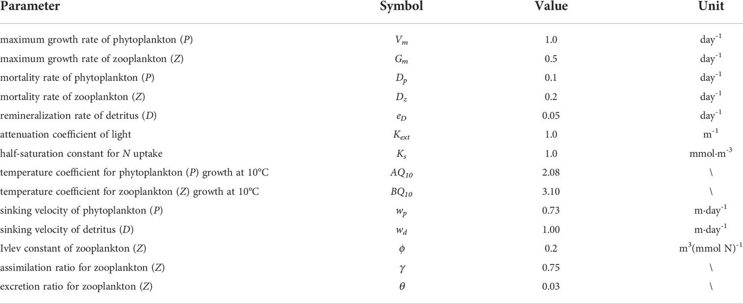
Table 1 The meaning and initial values of parameters in the marine ecological model.
The marine ecological equation (1) can be solved by several different numerical schemes. The central difference scheme is usually used in the adjoint assimilation method, but it is limited by the stability constraint and needs small time steps. To reduce the computation cost, we adopt a characteristic finite difference scheme that enables using large time steps. The variations of state variables (nitrogen (N), phytoplankton (P), zooplankton (Z), and detritus (D)) are small along the characteristic curve. Therefore, by computing along the characteristic direction, more accurate results of models can be obtained even using large time step sizes.
Let Δx , Δy and Δz be the spatial step size along x-, y-, and z-directions. The velocity U=(u(x,y,z), v(x,y,z), w(x,y,z) is given at the center of the grid. Δt is the time step. As shown in Figure 1, let be the concentration of the state variables at and tn=nΔt . Assuming that the concentration at each grid point at t = tn is known, we want to know the concentration at t=tn+1 . Let be the characteristic curve with the characteristic direction τ (Liang et al., 2016),
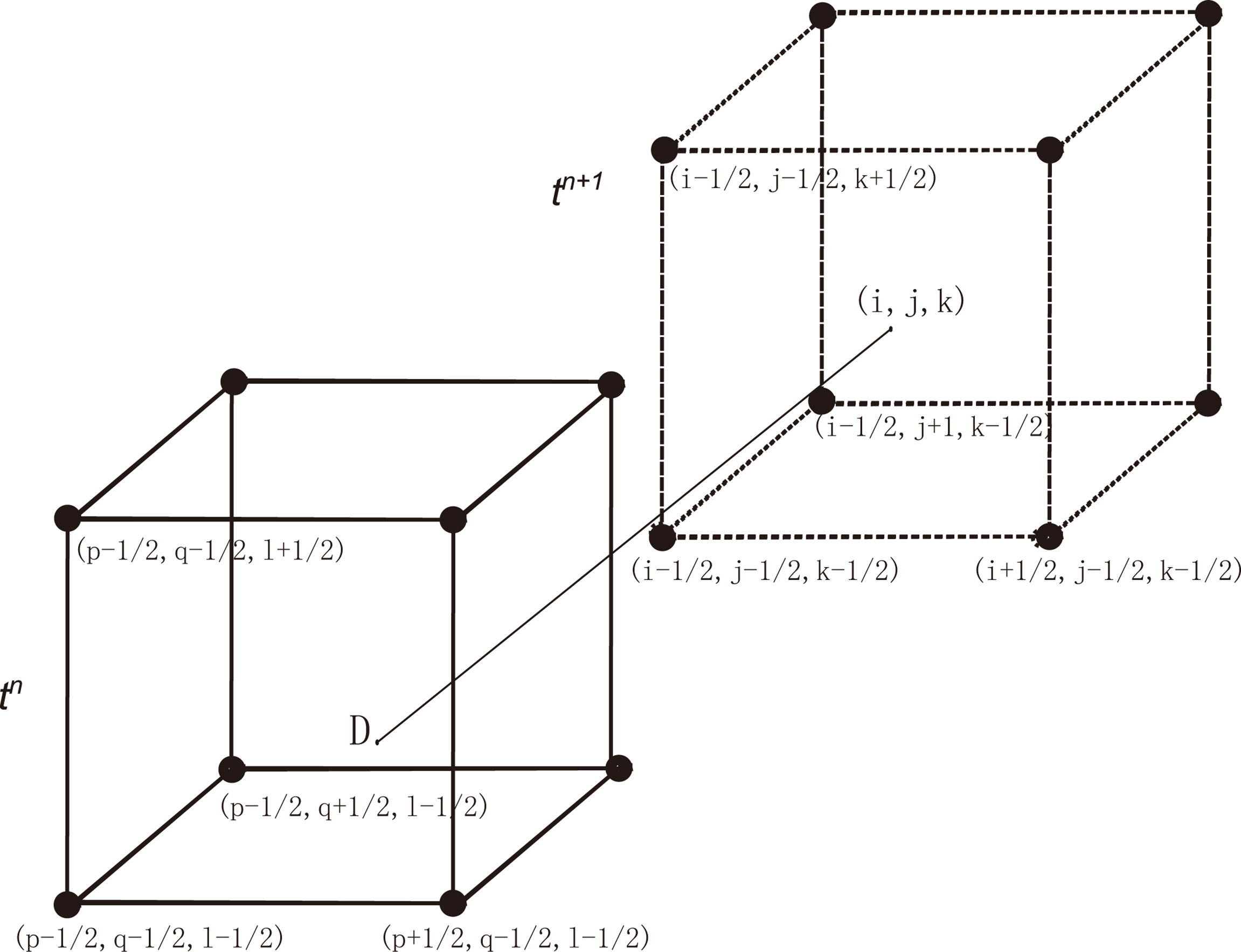
Figure 1 The process of constructing characteristic finite difference schemes.
Denote the intersection point of with the time level tn by (point D in Figure 1). We solve from the equations (7)-(8) by
The concentration at is determined by the interpolation of the values of the points surrounding Then the characteristic finite difference scheme is given as:
where
The adjoint model
According to the adjoint method, a cost function is defined to describe the difference between the simulated and observed surface phytoplankton:
where P is the simulated surface phytoplankton by the NPZD model and Pobs is the observed surface phytoplankton; Ω denotes the spatial domain and T is the time domain; K is the weighting matrix and the elements in K are 1 where observations are available and 0 otherwise. Rewrite equation (1),
where the parameters in the NPZD model are represented by . Based on the Lagrange multiplier method (Thacker and Long, 1988), the Lagrangian function is defined as:
where is the Lagrange multiplier of the state variables (nitrogen (N), phytoplankton (P), zooplankton (Z) and detritus (D)), respectively. Based on Lagrange multiplier theory, the first-order derivatives of the Lagrange function should be zero to minimize the cost function:
Equation (15) is equation (1) of the NPZD model. The adjoint equations can be derived from (16),
where the last term of each state variable’s Lagrange multipliers (Fan and Lv, 2009; Qi et al., 2011) is
We propose the characteristic finite difference schemes of (18)
where,
In the study of Fan and Lv (2009), the cost function is more sensitive to five constant parameters of Vm (maximum growth rate of phytoplankton), Gm (maximum grazing rate of zooplankton), Dp (mortality rate of phytoplankton), Dz (mortality rate of zooplankton) and eD (remineralization rate of detritus) by sensitivity analysis. Therefore, these five parameters are selected to be optimized. From equation (17), the gradients of the cost function concerning the five constant parameters (Fan and Lv, 2009; Qi et al., 2011) are obtained as follows:
When the gradients are calculated, the spatially varying parameters are estimated using the steepest descent method. The details are shown in Wang et al. (2020).
Numerical experiments
Numerical experiment 1: The Gaussian pulse moving
To test the performance of the characteristic finite difference scheme, the transport of a Gaussian hump was simulated by the characteristic finite difference scheme and the results were compared to those simulated by the central difference scheme.
In this subsection, the transport of the Gaussian pulse of the problem (1) with sms(C)=0 was considered. The spatial domain is Ω=[0,2]×[0,2] and time domain is t∈(0,0.2]. The initial condition is given by
where (x0,y0)=(0.3,0.3) , and the velocity is u=v=6 . The exact solution was
The diffusion coefficient is chosen as Aρ=0.001. Let Cn(x,y) denotes the approximate solution. The errors L∞ and L2 are defined as follows:
To examine the convergence rates in time of the characteristic finite difference scheme and central difference scheme, the small spatial step sizes Δx=Δy=1/500 and the time step sizes Δt=T/5,T/10,T/15,T/20 were carried out. The numerical results are presented in Table 2. When the large time steps were used, the results of the central difference scheme (CDS) were not stable. After adopting small time steps ( Δt=T/20000,T/21000,T/22000,T/23000 ), the stable results of CDS are listed in Table 2. It is clearly shown that the characteristic finite difference method (CFDM) and CDS exhibited a first-order ratio of convergence in time. Moreover, the L∞ and L2 errors of CFDM with the large time steps were less than those of CDS using the small time steps, indicating the high accuracy of CFDM. For example, when using Δt=T/5, the CFDM produced 7.5769×10⁻⁴ of E∞ and 6.2334×10⁻⁵ of E2, while the E∞ and E2 of CDS using Δt=T/20000 were 1.3394×10⁻² and 1.4925×10⁻³, respectively.To further explore the effectiveness of CFDM, the transport of the Gaussian pulse of the problem (1) with sms(C)=0 in three-dimensional space was considered. The initial condition is given as:
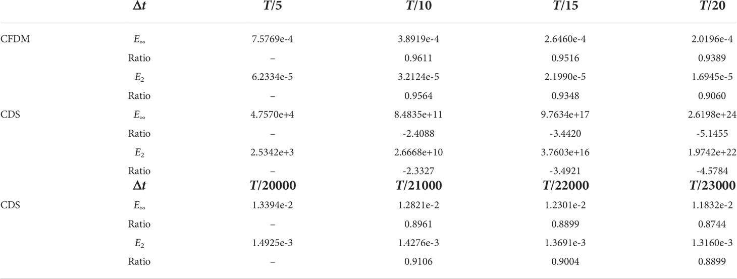
Table 2 Errors and ratios in time of the 2D Gaussian pulse for the experiment using large time steps by the CFDM and CDS method and using small time steps calculated by the CDS method.
The exact solution of the problem is
where, the spatial domain is Ω=[0,2]×[0,2]×[0,2], the initial center is (x0,y0,z0)=(0.5,0.5,0.5), the velocity is (u,v,w)=(0.8,0.8,0.1), and the diffusivity coefficient is Aρ=Kρ=0.01. The spatial step sizes were taken as Δx=Δy=Δz=0.025. The time step size for CFDM was Δt=0.0625. With the limit of stability, a smaller time step size of Δt=0.00625 was set for CDS.
A group of surfaces obtained by CFDM and CDS in the section of y=x and contour plots at z = 0.6 at different times of t= 0.75, 1, and 1.25, which displayed the concentration distributions are shown in Figures 2, 3. The results calculated by CFDM almost coincided with the exact solutions and were more accurate than those of CDS with 10 times smaller time step, indicating that the Gaussian pulse could be simulated by CFDM very well even using a much large time step. Furthermore, the computed peaks and numerical errors in L∞ and L2 norms at different times shown in Table 3 demonstrated that the model performance was improved by CFDM. For example, at time t=1.25, where the maximum value of the exact solution was 0.0675, the computed peak of CFDM was 0.0707, while that of CDS was 0.0827. Besides, at time t=1.25, the errors of CFDM were 3.1538×10⁻³ in L∞ -norm and 1.7879×10⁻³ in L2-norms, which were one order of magnitude smaller than those of CDS ( 1.5155×10⁻² in L∞ -norm and 1.3649×10⁻² in L2 -norm). Overall, the simulation results of CFDM were much closer to the exact solutions than those of CDS, demonstrating that CFDM could significantly improve the model performance.
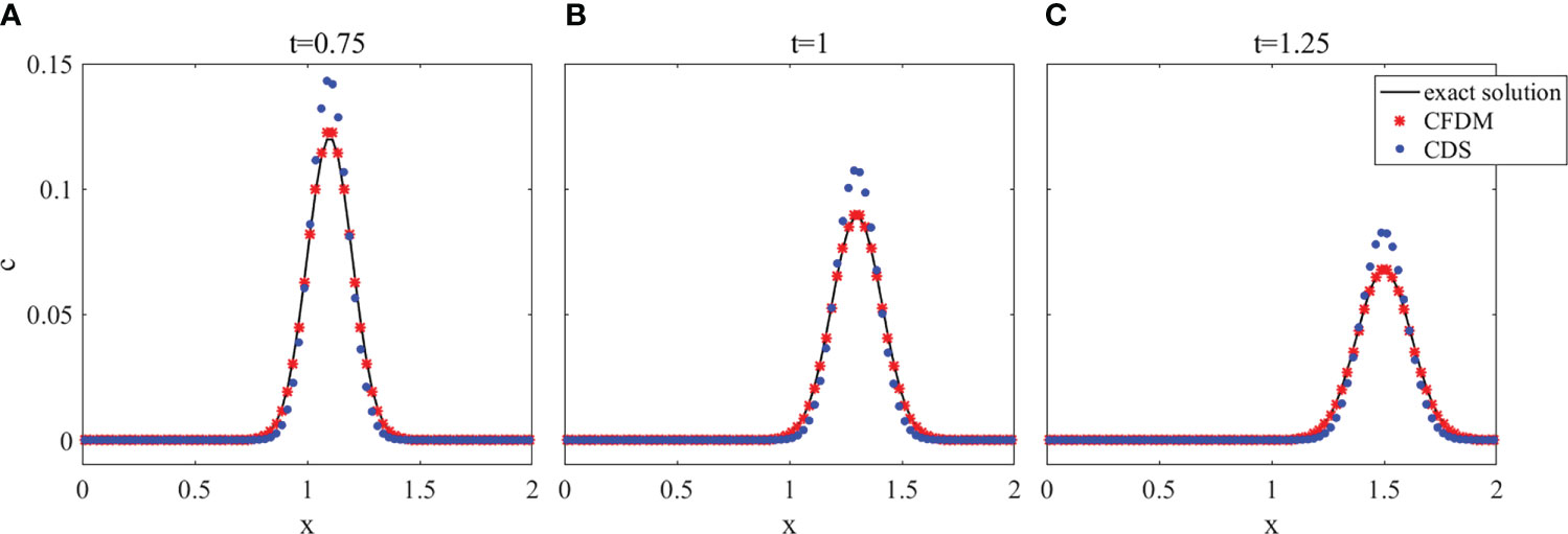
Figure 2 The surface plots in the section of y = x of the 3D Gaussian hump at z = 0.6 with different times. (A) t=0.75, (B) t=1, (C) t=1.25.
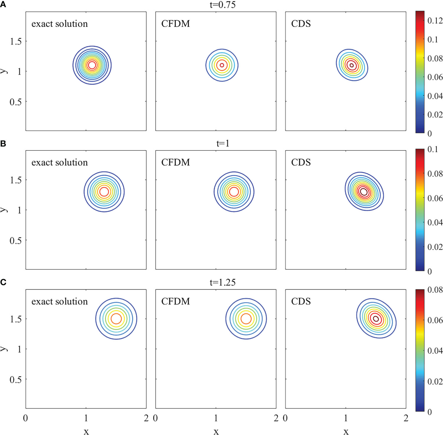
Figure 3 The contour plots of the 3D Gaussian hump at z = 0.6 with different times (A) t=0.75, (B) t=1, (C) t=1.25.
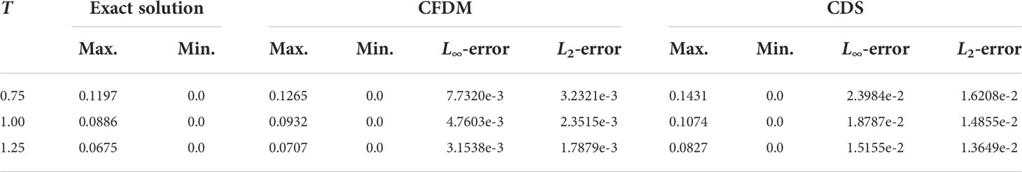
Table 3 The maximum and minimum values and errors of the 3D moving Gaussian pulse.
Numerical experiment 2: Parameter optimization of NPZD model
In this subsection, the adjoint assimilation method combining with CFDM was used to optimize the spatial parameters SP (Vm, Gm, Dp, Dz, eD). The process of the numerical experiment can be described as:
Step 1. Give the guess of distribution of parameters SP 0 as the initialization of parameters.
Step 2. For n = 0, 1, ..., N (the number of iterations), do Step 3-Step 5.
Step 3. With the initial distribution of parameters SP n, solve the NPZD model and get simulated results.
Step 4. Solve the cost function (12) by the simulations and observations. If the cost function decreases to 10-5, exit the loop and run Step 6.
Step 5. Run the adjoint model backward in the time direction and calculate the gradient of the cost function on the parameters SP n. Then get the optimized parameters SP n+1 by adjusting SP n with the steepest descent method.
Step 6. Output the final optimized parameters.
Experiment design
The studied region (24°N–41°N,117.5°E–131°E) covers the Bohai Sea, the Yellow Sea, and the East China Sea. The horizontal resolution is 10′×10′ with grid numbers of 103 (south-north) ×82 (west-east). The vertical direction is 6 layers and the thickness of each layer from top to bottom is 10m, 10m, 10m, 20m, 25m, and 25m respectively. The data over the simulation period, such as the ambient physical velocities, the temperature, and eddy diffusivities, etc., were interpolated to the vertical grid using the results obtained by the three-dimensional Princeton Ocean Model (POM) (Blumberg and Mellor, 1987). In addition, river sources of Changjiang (http://xxfb.hydroinfo.gov.cn) were added to the model. The initial fields of nitrogen and phytoplankton were converted from monthly mean nitrate of World Ocean Atlas 2013 (WOA13) and monthly mean surface chlorophyll-a concentrations of SeaWiFS, respectively. The starting time was 1 January 2016. Besides, the NPZD model was run for 30 days for spin-up to obtain the initial fields of zooplankton and detritus. Then the adjoint model was run for 5 days backward in time from 1 February 2016 with the spin-up ocean state as the initial conditions.
During the experiment, four state variables of the marine ecological model of nitrogen (N), phytoplankton(P), zooplankton (Z), and detritus (D) were converted to nitrogen units( mmol N·m-3 ). For the NPZD model, satellite chlorophyll-a data ( mg·m-3 ) of SeaWiFS was converted to nitrogen units ( mmol N·m-3 ) using an equation (36) of the relation between chlorophyll-a and carbon proposed by Semovski and Wozniak (1995) and a constant phytoplankton carbon-to-nitrogen Redfield ratio (Redfield et al., 1963; Faugeras et al., 2004)
where ρmax=90 and the half-saturation coefficient is K1/2=0.477 As indicated by Moisan et al. (2002), the parameters of the marine ecological model were related to temperature. Therefore, according to the initial values of parameters listed in Table 1 and the trend of the surface temperature field, two types of parameters were given to verify the accuracy of the adjoint data assimilation with CFDM.
Type 1:
Type 2:
where α0 was the initial value of the parameter shown in Table 1.
Single parameter inversion
To test the effectiveness of the adjoint data assimilation with CFDM, the experiments of single parameter inversion were carried out. In these experiments, one of the five parameters (Vm, Gm, Dp, Dz, eD) was assumed to vary spatially by Type 1 or Type 2, and the other four parameters were constants in Table 1. The NPZD model was run for 5 days from 1 February 2016 and the time step was Δt = 6h. During the experiment, only the parameter with given spatial distributions was inversed, and initial guesses were set as the default values shown in Table 1. The observations used were the simulated concentrations of phytoplankton by the NPZD model with five assumed parameters. The calculated mean absolute errors (MAE) and mean relative errors (MRE) between the given parameter and the corresponding inversed parameter values are listed in Table 4. When the time step size was set to 6h, the numerical oscillations occurred in CDS and the MAE and MRE were one order of magnitude larger than those of CFDM. Therefore, the experiment of CDS (Δt = 30min) was carried out.
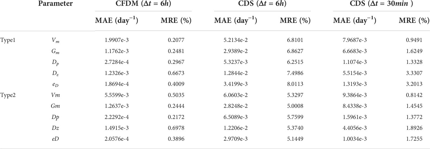
Table 4 The errors between the inversion results and the given parameters in the experiment of optimizing parameters separately.
As listed in Table 4, the MAEs between the inverted parameters (Vm, Gm, Dp, Dz, eD) and the spatial values varying as Type 1 of CFDM (Δt = 6h) were 1.9907×10⁻³ , 1.1762×10⁻³ , 2.7284×10⁻⁴ , 1.2326×10⁻³ ,and 1.8694 ×10⁻⁴ day−1, respectively; the MAEs of CDS ( Δt=30min ) were much larger values of 7.9687×10⁻³, 6.6683×10⁻³, 1.1074×10⁻³, 5.5154×10⁻³, and 1.3193×10⁻³ day−1, respectively. The mean MRE of the five parameters between the given Type1 and corresponding inverted results was reduced to 0.36 % in CFDM ( Δt=6h ) from 2.09 % in CDS ( Δt=30min ). Similar results could also be obtained in the Type2 experiments, indicating that the model performance was improved by CFDM even using large time steps.
Simultaneous inversion of five parameters
As indicated by Li et al. (2013), the distributions of Vm, Dz, and eD were consistent and Gm and Dp had a similar distribution. Therefore, the five parameters were supposed to be spatially varying, which were estimated synchronously. In this subsection, the values of Vm, Dz, eD were assumed to vary spatially by Type1, Gm, and Dp were distributed by Type 2. The observations used for data assimilation were the simulated concentrations of phytoplankton by the NPZD model with five assumed parameters. To verify the effect of data assimilation with CFDM, the data assimilation was implemented using CFDM with Δt=6h and CDS with Δt=30min, and the initial guess values of the five parameters were set to the default values shown in Table 1 in Case 1.
In addition, previous studies have indicated that reasonable initial guesses of target parameters can accelerate the optimization rate and improve the simulations. Therefore, the sensitivity analysis of the initial parameter values was designed in this subsection. The initial parameter values were set as 0.8 and 1.2 of the default values shown in Table 1 in Case 2 and Case 3. The distributions of inversion results and given parameters are shown in Figure 4. The estimated results of the three experiments were all in good agreement with the prescribed parameters. The cost function normalized by the value at the first iteration step was shown in Figure 5. The normalized cost functions of CFDM in Case 1 to Case 3 were both reduced by at least three orders of magnitude, which dropped faster than those of CDS. However, compared to Case 2 and Case 3, Case 1 had the highest efficiency of convergence, and only 42 iteration steps were used to reach the minimum. Consequently, the initial guess had a great impact on the efficiency of convergence and should be reasonably selected. In the following experiments, the initial guesses were all set as the default values shown in Table 1.
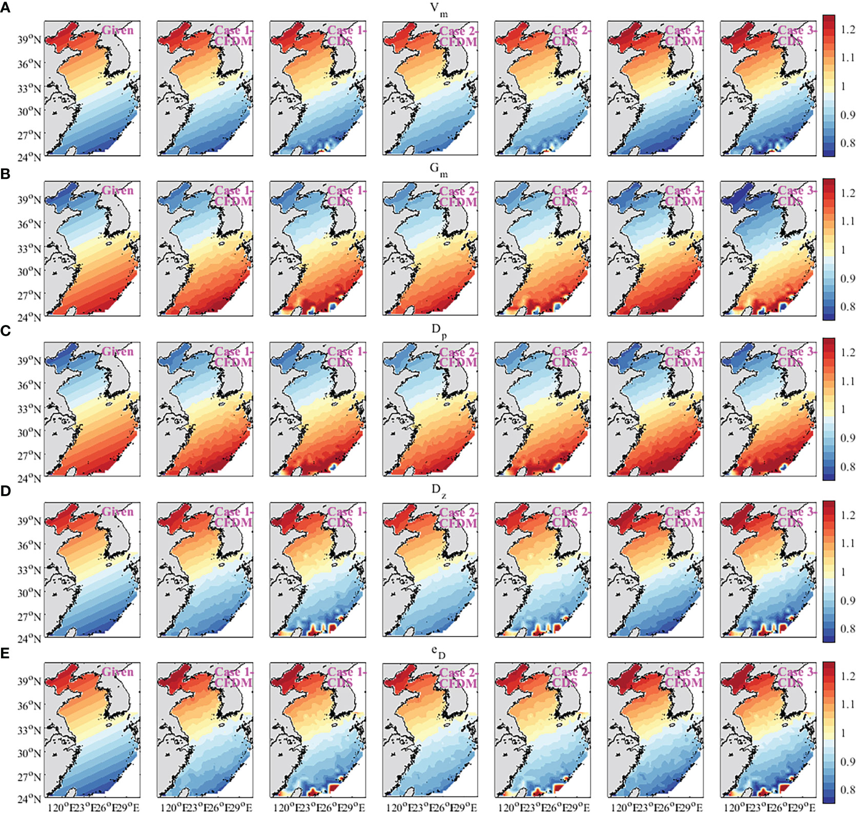
Figure 4 Spatial variation of five inversion parameters in the experiment of optimizing parameters simultaneously (unit: day−1). (A) Vm, (B) Gm, (C) Dp, (D) Dz, and (E) eD.
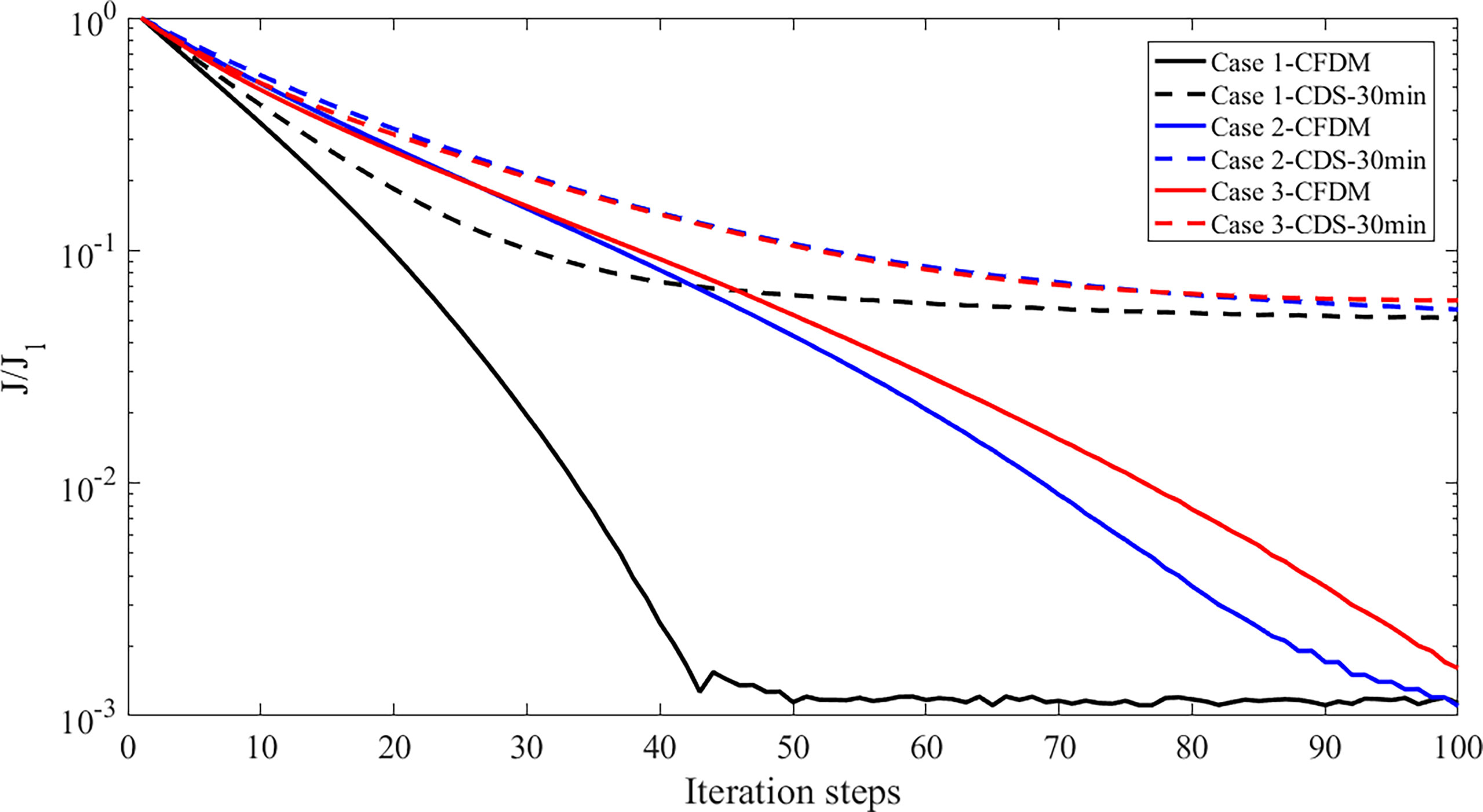
Figure 5 The values of the normalized cost function (J/J1) versus the iteration steps.
The errors in Case 1 are listed in Table 5. The inversed parameters after data assimilation with CFDM and CDS had similar spatial features with the given values, in which the high errors of CDS were near the south boundaries; conversely, the estimated parameters of CFDM were consistent with the given spatial variations. Besides, in CDS ( Δt=30min ), the MAEs between the inverted parameters (Vm, Gm, Dp, Dz, eD) and the spatial values were increased to 8.0097×10⁻³, 1.0031×10⁻², 1.6888×10⁻³, 5.1425×10⁻³, and 1.3063×10⁻³ day−1, respectively, which were larger than 3.1432×10⁻³, 4.6792×10⁻³, 9.5625×10⁻⁴, 1.4997×10⁻³, and 6.1339×10⁻⁴ day−1 of CFDM ( Δt=6h). The mean MRE of the five parameters was reduced to 0.88 % by CFDM ( Δt=6h ) from 2.08 % by CDS ( Δt=30min ).
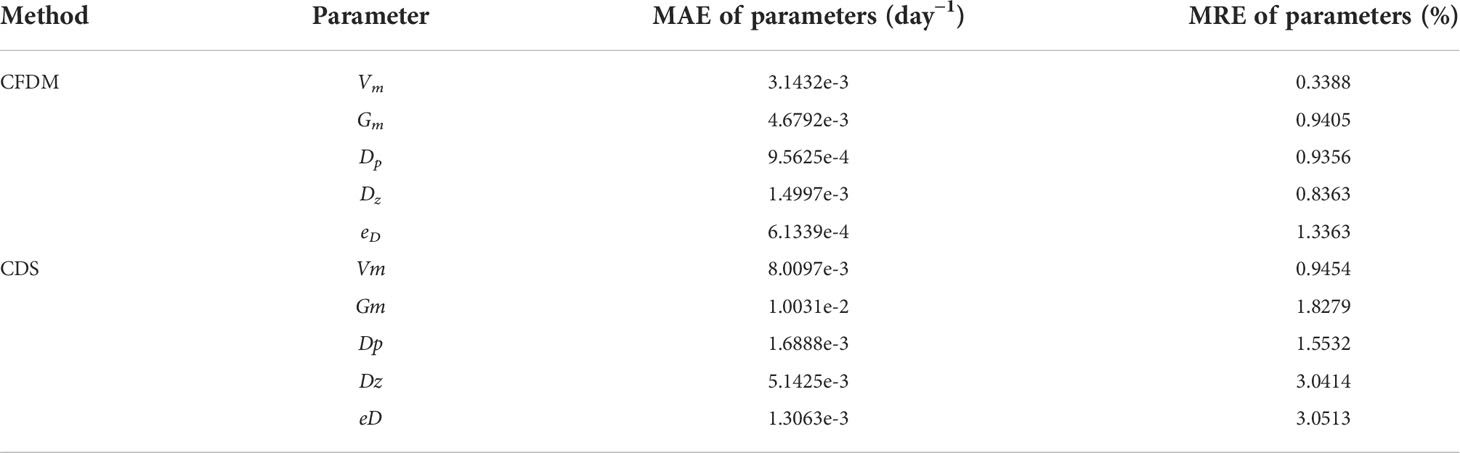
Table 5 Same as Table 4, but for the experiment of Case 1 of optimizing parameters simultaneously.
In addition, The MAE between simulated chlorophyll-a and observations and running time of CFDM and CDS in Case 1 are listed in Table 6. For CFDM, the normalized cost function was less than 0.0016 after running 1351.55 s. For CDS, the normalized cost function was less than 0.0826 after running 26697.83 s. The MAE between the simulated phytoplankton and chlorophyll-a was 0.2434 mmol N·m-3 (0.2823 mmol N·m-3) before data assimilation in CFDM (CDS); after assimilation, the MAE was decreased to 0.0036 mmol N·m-3 (0.0197 mmol N·m-3) in CFDM (CDS), indicating that the model performance was improved with a reduction of 98.52 % (93.02 %) in overall simulation error. Using about 1/30 of the time of the CDS method, more accurate results were obtained by CFDM, which further shows that CFDM can optimize five parameters efficiently.
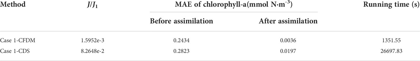
Table 6 The J/J1, MAE of chlorophyll-a and running time assimilated by different methods.
Influence of errors of observations
In all the above experiments, the observations of chlorophyll-a were perfect without errors. However, in practice, there might be 20%-30% errors in the chlorophyll-a concentrations obtained by SeaWiFS (Gregg and Casey, 2004; Cui et al., 2014), due to its digitization round-off and noise errors (Hu et al., 2001). If the available observations are not accurate, the estimation of parameters might not conform to the actual distribution. Thus, it is necessary to discuss the influence of observation errors on the estimated parameters. To partly reflect reality, the observations over random error within ±20%, ±30%, ±35%, and ±40% were considered in Case 4 to Case 7. In these experiments, the values of Vm, Dz and eD were assumed to vary spatially by Type1, Gm and Dp were distributed by Type 2. During the experiment, five parameters were inversed simultaneously and initial guesses was set as the default values shown in Table 1. The observations used for data assimilation were the simulations of phytoplankton by the NPZD model with five assumed parameters with ±20%, ±30%, ±35%, and ±40% random errors.For experiments of Case 4 to Case 7, when the percentage error became larger, the estimated results worsened (Figure 6). With the 30% errors, the estimated results in CFDM ( Δt=6h ) were close to the prescribed parameters, and the high values of errors only occurred near the boundary. There were lots of misfits between the estimated results in CDS ( Δt=30min ) and the prescribed parameters. When the maximum percentage of errors was up to 35%, the estimations of eD differed greatly from prescribed eD. When the maximum percentage of errors was up to 40%, the estimations of Gm differed greatly from the prescribed Gm.
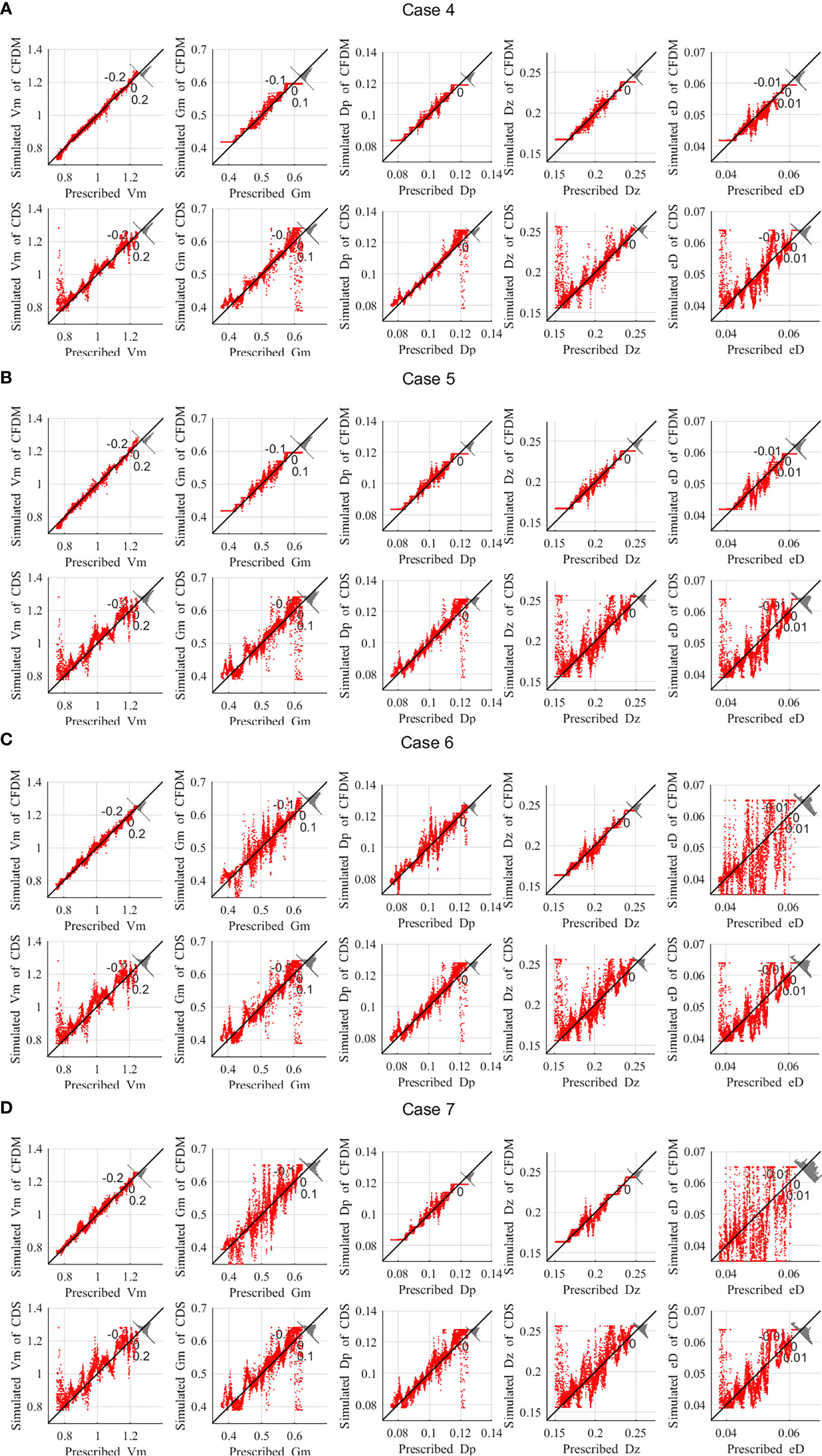
Figure 6 Comparison of the five parameters obtained by the CFDM and CDS method and the prescribed values in (A) Case 4, (B) Case 5, (C) Case6, (D) Case 7. This image shows the misfits between the estimations and their real values. (unit: day−1).
As listed in Table 7, with the 30% errors, the estimated parameters contained more errors than in experiments without observation errors, where the maximum MRE of CFDM (Δt=6h) between the estimated results and the prescribed parameters decreased from 1.34% to 2.92%, indicating that the estimated parameters were still acceptable. The errors of CFDM were smaller than those of the CDS method. For example, the MAE and MRE of Vm obtained by CFDM were 9.6420×10⁻³ day-1 and 1.0184% respectively, while those of the CDS method were 3.0106×10⁻²day-1 and 3.2083%. Based on this analysis, we concluded that the degree of errors of chlorophyll-a obtained by SeaWiFS used in this paper was acceptable and the present model and method could partly bear the influence of errors of observations.

Table 7 Same as Table 5, but for the experiment of Case 5 with 30% observation errors.
Practical experiments and results analysis
In practical experiments, the monthly mean climatological SeaWiFS data of the period 1997-2016 were interpolated into daily data and the daily SeaWiFS data (Sathyendranath et al., 2020) was used to correct the interpolated data. These observations were assimilated to optimize the parameters (Vm, Gm, Dp, Dz, eD) and to improve simulation results. The CFDM was selected in the optimization algorithm. The initial conditions of nitrogen and phytoplankton were obtained through spatial interpolation of the WOA13 and SeaWiFS data measured at the initial time. Because of the lack of the distributions of zooplankton and detritus, the NPZD model was run for one months from December 1st, 2015 to January 1st, 2016, in which the initial guesses of zooplankton and detritus in the surface layer were 0.2 and 0.1 mmol N·m-3 and the concentration decreased exponentially with the increase of depth P(k)=P(1)e-(z(k)-z(1))/zch (k=1,2,…,6), with zch = 100m (Losa et al., 2006). The remaining model parameters were set as default empirical values (Table 1). Then the simulated results were taken as the initial conditions to optimize five parameters in 2016.
Figure 7 depicts the seasonal means of the five parameters (Vm, Gm, Dp, Dz, eD), estimated in the practical experiments. The estimated distributions of the five parameters showed a seasonal cycle. The relatively high values of Vm, Gm and Dp appeared in winter, then decreased through the spring and summer, and increased again during autumn. Conversely, The Dz and eD increased in spring and summer and decreased in autumn. In winter, high values of the maximum growth rate of phytoplankton (Vm) appeared in the near seas (~12 nautical miles territorial seas) north of 34°N. The nutrient concentrations varied seasonally and the highest concentrations of dissolved inorganic nitrogen, dissolved inorganic phosphorus, and dissolved silicate in the Bohai Sea was in winter (Zheng et al., 2020; Ding et al., 2021). Therefore, the values of Vm were large in the Bohai Sea, especially in Liaodong Bay. Previous studies showed that temperature had a great effect on zooplankton in the Yellow Sea during winter (Chen et al., 2011; Shi et al., 2018). Affected by the Yellow Sea Warm Current, Taiwan Warm Current, and Kuroshio, the values of Gm (maximum growth rate of zooplankton) were large in the East China Sea and the middle of the Yellow Sea.
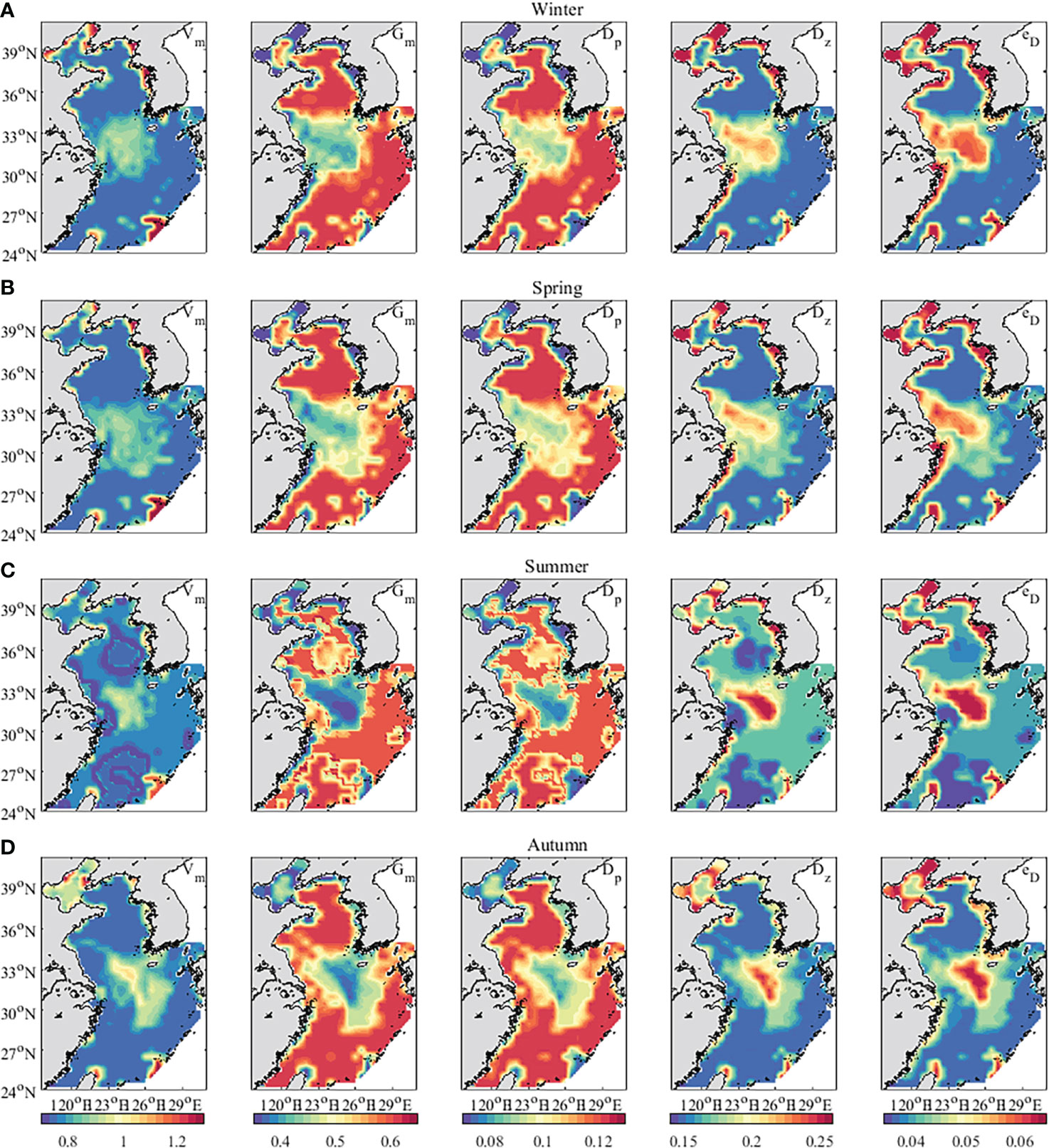
Figure 7 The distribution of five parameters inverted by the CFDM (unit: day−1). (A) Winter (Jan-Mar); (B) Spring (Apr-Jun); (C) Summer (Jul-Sep); (D) Autumn (Oct-Dec).
Besides, based on the inversion results, the correlation coefficients (R) between the five parameters were calculated. There were strong correlations between Vm, Dz, and eD, in which R of Vm and Dz were 0.73, 0.67, 0.81 and 0.77, respectively, R of Vm and eD were 0.69, 0.63, 0.75, and 0.76, respectively, and R of Dz and eD were 0.92, 0.92, 0.93, and 0.96, respectively, in different seasons. Gm and Dp were strongly related. R of Gm and Dp were 0.90, 0.89, 0.94, and 0.89 respectively, in different seasons. The result is consistent with the actual situation. When zooplankton increased, the concentrations of phytoplankton would decrease. Therefore, Gm and Dp (mortality rate of phytoplankton) change consistently. The concentrations of phytoplankton and detritus increased as zooplankton mortality increased. The Vm and eD (remineralization rate of detritus) would vary with Dz (mortality rate of zooplankton).
To further verify the accuracy of the result, the distributions of phytoplankton simulated by the NPZD model with optimized parameters were compared with those of the NPZD model without optimized parameters. In the data assimilation experiment, one-tenth of the observation data randomly selected were not assimilated and used as independent observation to test the results, which was called ‘test observation’. The seasonal sea surface phytoplankton obtained from SeaWiFS data, simulated by the NPZD model without optimized parameters and the NPZD model without optimized parameters are shown in Figure 8. Compared with the observations of SeaWiFS data, the results simulated by the NPZD model with optimized parameters matched the real data. The MAEs between the simulation of the NPZD model with optimized parameters and the test observation were 0.45, 0.50, 0.49 and 0.40 mmol N·m-3 in winter, spring, summer and autumn, respectively, which were smaller than 1.01, 1.24, 2.18 and 0.97 mmol N·m-3 of the NPZD model without optimized parameters.
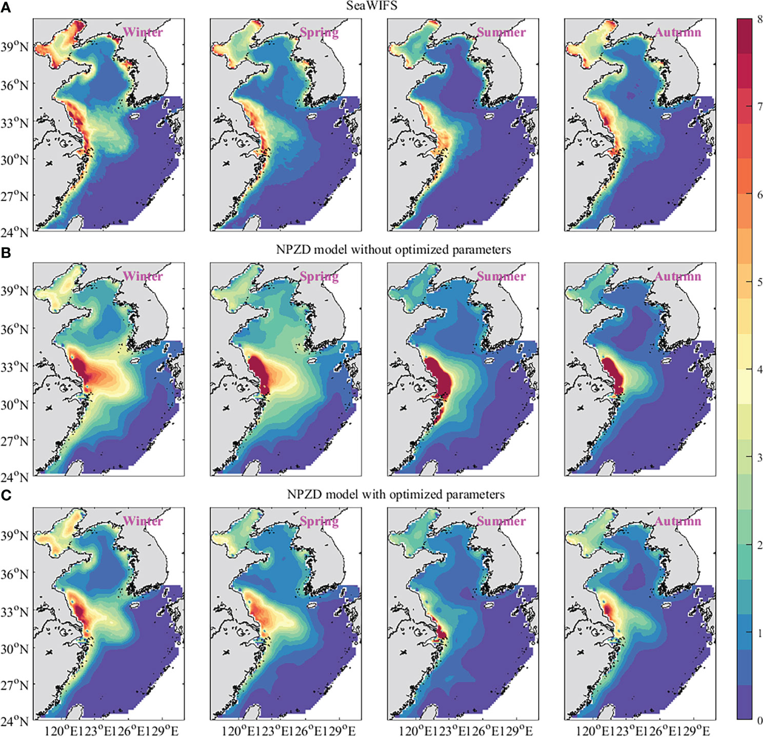
Figure 8 The sea surface phytoplankton obtained from SeaWiFS data (A), simulations of the NPZD model without optimized parameters (B) and simulations of the NPZD model without optimized parameters (C). (unit: mmol N·m-3).
The seasonal observations and simulations of the average value of phytoplankton on the sea surface are shown in Figure 8. The simulations reproduced the concentrations of the sea surface phytoplankton and the seasonal cycle where the high values appeared in winter and then decreased through the spring and summer, and increased again during autumn. This variety tendency was the same as that of Vm. The microbiology points out that the maximum growth rate occurs when the population density is optimum (Weaver and Grime, 1980). Once the population density is larger than the optimum density, the growth rate will reduce because of the limited nutrient and environmental conditions. The estimations of Vm implied that there was a connection between the growth rate and the phytoplankton concentration. The experiments show that the adjoint assimilation method with CFDM can invert the parameter values in the ecosystem model very well using large time steps.
Conclusions
Based on the adjoint data assimilation method with CFDM, the estimation of the parameters of the NPZD model is studied in this paper. The CFDM reduced the calculation time by large time steps and generated accurate numerical solutions. The experiment of the Gaussian pule moving shows the effectiveness of CFDM. Further, a series of experiments are carried out to evaluate the adjoint data assimilation method with CFDM and CDS and to examine the influential factors on the inversions of the five parameters (Vm, Gm, Dp, Dz, eD) by assimilating the chlorophyll-a concentrations obtained by the SeaWiFS data. Considering the inversion errors and convergence rates synthetically, the CFDM performs better than CDS. Whether the five parameters were optimized separately or simultaneously, the parameters obtained by CFDM were more consistent with the distribution of the given parameters. The errors in observations have little influence on the estimated results, and the estimated results are all satisfactory, indicating that this model has a strong parameter estimation ability. According to the results of the twin experiments, the adjoint data assimilation method with CFDM is applied in a practical experiment to estimate the five parameters in February 2016. The results indicate that the improved data assimilation method can optimize the parameter values in the ecosystem model efficiently and the CFDM which gets rid of the limitation of stability provides an efficient choice for the study of high resolution model. Future work will focus on the optimization of parameters of the NPZD model in larger areas, longer time scales, and extreme weather conditions using the adjoint method, thus further improving the numerical simulations of the marine ecosystem.
Data availability statement
The raw data supporting the conclusions of this article will be made available upon reasonable request and with authors’ permission. Open source datasets, includes World Ocean Atlas 2013 (WOA13; available online at https://www.nodc.noaa.gov/OC5/woa13) and Sea-Viewing Wide Field-of-View Sensor (SeaWIFS; available online at https://seawifs.gsfc.nasa.gov/ and https://esa-oceancolour-cci.org/).
Author contributions
MX conducted the data analysis, software, model validation, writing, and visualization. YL, KF, and XL conducted the formal analysis, software, and supervision. ZZ prepared the formal analysis and model validation. All authors contributed to the article and approved the submitted version.
Funding
This work was supported by the National Natural Science Foundation of China 42106146, the Natural Science Foundation of Shandong Province of China ZR2021MA005 and ZR2020MD056, and the National Natural Science Foundation of China (Grant No. 11601497, 42076011 and U1806214).
Acknowledgments
We acknowledge all the reviewers for their valuable suggestions.
Conflict of interest
The authors declare that the research was conducted in the absence of any commercial or financial relationships that could be construed as a potential conflict of interest.
Publisher’s note
All claims expressed in this article are solely those of the authors and do not necessarily represent those of their affiliated organizations, or those of the publisher, the editors and the reviewers. Any product that may be evaluated in this article, or claim that may be made by its manufacturer, is not guaranteed or endorsed by the publisher.
Supplementary material
The Supplementary Material for this article can be found online at: https://www.frontiersin.org/articles/10.3389/fmars.2022.997537/full#supplementary-material
References
Anderson D. A., Tannehill J. C., Pletcher R. H. (1984) Computational fluid mechanics and heat transfer Comput. fluid Mech. heat Transf. (Hemisphere Pub. Corp.) 1(4),101–234. doi: 10.2307/2008017
Arbogast T., Huang C., Zhao X., King D. N. (2020). A third order, implicit, finite volume, adaptive runge–kutta WENO scheme for advection–diffusion equations. Comput. Methods Appl. Mech. Eng. 368. doi: 10.1016/j.cma.2020.113155
Ascher U. M., Ruuth s. J., Wetton B. T. R. (1995). Methods for time dependent partial differential equations. SIAM J. Numer. Anal. 32, 797–823. doi: 10.1090/psapm/022/533052
Athias V., Mazzega P., Jeandel C. (2000). Selecting a global optimization method to estimate the oceanic particle cycling rate constants. J. Mar. Res. 58, 675–707. doi: 10.1357/002224000321358855
Baba K., Tabata M. (1981). On a conservation upwind finite element scheme for convective diffusion equations. RAIRO. Anal. numérique 15, 3–25. doi: 10.1051/m2an/1981150100031
Blumberg A. F., Mellor G. L. (1987). A description of a three-dimensional coastal ocean circulation model. Three-Dimens. Coast. Model. Coast. Estuar. Ser., 1–16. doi: 10.1029/co004p0001
Borja A., Andersen J. H., Arvanitidis C. D., Basset A., Buhl-Mortensen L., Carvalho S., et al. (2020). Past and future grand challenges in marine ecosystem ecology. Front. Mar. Sci. 7. doi: 10.3389/fmars.2020.00362
Chen H., Qi Y., Liu G. (2011). Spatial and temporal variations of macro- and mesozooplankton community in the huanghai Sea (Yellow Sea) and East China Sea in summer and winter. Acta Oceanol. Sin. 30, 84–95. doi: 10.1007/s13131-011-0108-5
Cui T., Zhang J., Tang J., Sathyendranath S., Groom S., Ma Y., et al. (2014). Assessment of satellite ocean color products of MERIS, MODIS and SeaWiFS along the East China coast (in the yellow Sea and East China Sea). ISPRS J. Photogramm. Remote Sens. 87, 137–151. doi: 10.1016/j.isprsjprs.2013.10.013
Ding X., Guo X., Gao H., Gao J., Shi J., Yu X., et al. (2021). Seasonal variations of nutrient concentrations and their ratios in the central bohai Sea. Sci. Total Environ. 799, 149416. doi: 10.1016/j.scitotenv.2021.149416
Douglas J. Jr., Russell T. F. (1982). Numerical methods for convection-dominated diffusion problems based on combining the method of characteristics with finite element or finite difference procedures. SIAM J. Numer. Anal. 19, 871–885. doi: 10.1137/0719063
Ebrahimijahan A., Dehghan M., Abbaszadeh M. (2020). Compact local integrated radial basis functions (Integrated RBF) method for solving system of non–linear advection-diffusion-reaction equations to prevent the groundwater contamination. Eng. Anal. Bound. Elem. 121, 50–64. doi: 10.1016/j.enganabound.2020.09.003
Fan W., Lv X. (2009). Data assimilation in a simple marine ecosystem model based on spatial biological parameterizations. Ecol. Modell. 220, 1997–2008. doi: 10.1016/j.ecolmodel.2009.04.050
Faugeras B., Bernard O., Sciandra A., Lévy M. (2004). A mechanistic modelling and data assimilation approach to estimate the carbon/chlorophyll and carbon/nitrogen ratios in a coupled hydrodynamical-biological model. Nonlinear Process. Geophys. 11, 515–533. doi: 10.5194/npg-11-515-2004
Franks P. J. S. (2002). NPZ models of plankton dynamics: Their construction, coupling to physics, and application. J. Oceanogr. 58, 379–387. doi: 10.1023/A:1015874028196
Franks P. J. S., Chen C. (2001). A 3-d prognostic numerical model study of the georges bank ecosystem. part II: Biological-physical model. Deep. Res. Part II Top. Stud. Oceanogr. 48, 457–482. doi: 10.1016/S0967-0645(00)00125-9
Friedrichs M. A. M. (2001). Assimilation of JGOFS EqPac and SeaWiFS data into a marine ecosystem model of the central equatorial pacific ocean. Deep. Res. Part II Top. Stud. Oceanogr. 49, 289–319. doi: 10.1016/S0967-0645(01)00104-7
Fu K. A. I., Liang D. (2019). A mass-conservative temporal second order and spatial fourth order characteristic finite volume method for atmospheric pollution advection diffusion problems. SIAM J. Sci. Comput, 41, B1178–B1210. doi: 10.1137/18M121914X.
Fu K., Liang D., Wang W., Cui M. (2015). The time second-order characteristic fem for nonlinear multicomponent aerosol dynamic equations in environment. Int. J. Numer. Anal. Model. 12, 211–229.
Gao X., Wei Z., Lv X., Wang Y., Fang G. (2015). Numerical study of tidal dynamics in the south China Sea with adjoint method. Ocean Model. 92, 101–114. doi: 10.1016/j.ocemod.2015.05.010
Gharamti M. E., Tjiputra J., Bethke I., Samuelsen A., Skjelvan I., Bentsen M., et al. (2017). Ensemble data assimilation for ocean biogeochemical state and parameter estimation at different sites. Ocean Model. 112, 65–89. doi: 10.1016/j.ocemod.2017.02.006
Gregg W. W., Casey N. W. (2004). Global and regional evaluation of the SeaWiFS chlorophyll data set. Remote Sens. Environ. 93, 463–479. doi: 10.1016/j.rse.2003.12.012
Gunson J., Oschlies A., Garçon V. (1999). Sensitivity of ecosystem parameters to simulated satellite ocean color data using a coupled physical-biological model of the north Atlantic. J. Mar. Res. 57, 613–639. doi: 10.1357/002224099321549611
Heinle A., Slawig T. (2013). Internal dynamics of NPZD type ecosystem models. Ecol. Modell. 254, 33–42. doi: 10.1016/j.ecolmodel.2013.01.012
Hu C., Carder K. L., Muller-Karger F. E. (2001). How precise are SeaWiFS ocean color estimates? implications of digitization-noise errors. Remote Sens. Environ. 76, 239–249. doi: 10.1016/S0034-4257(00)00206-6
Jones E. M., Baird M. E., Mongin M., Parslow J., Skerratt J., Lovell J., et al. (2016). Use of remote-sensing reflectance to constrain a data assimilating marine biogeochemical model of the great barrier reef. Biogeosciences 13, 6441–6469. doi: 10.5194/bg-13-6441-2016
Kishi M. J., Kashiwai M., Ware D. M., Megrey B. A., Eslinger D. L., Werner F. E., et al. (2007). NEMURO-a lower trophic level model for the north pacific marine ecosystem. Ecol. Modell. 202, 12–25. doi: 10.1016/j.ecolmodel.2006.08.021
Kuhn A. M., Fennel K., Mattern J. P. (2015). Model investigations of the north Atlantic spring bloom initiation. Prog. Oceanogr. 138, 176–193. doi: 10.1016/j.pocean.2015.07.004
Kurganov A., Tadmor E. (2000). New high-resolution central schemes for nonlinear conservation laws and convection-diffusion equations. J. Comput. Phys. 160, 241–282. doi: 10.1006/jcph.2000.6459
Kytinou E., Sini M., Issaris Y., Katsanevakis S. (2020). Global systematic review of methodological approaches to analyze coastal shelf food webs. Front. Mar. Sci. 7. doi: 10.3389/fmars.2020.00636
Lawson L. M., Hofmann E. E., Spitz Y. H. (1996). Time series sampling and data assimilation in a simple marine ecosystem model. Deep. Res. Part II Top. Stud. Oceanogr. 43, 625–651. doi: 10.1016/0967-0645(95)00096-8
Lax P. D. (1954). Weak solutions of nonlinear hyperbolic equations and their numerical computation. Commun. Pure Appl. Math. 7, 159–193. doi: 10.1002/cpa.3160070112
Liang D., Fu K., Wang W. (2016). Modelling multi-component aerosol transport problems by the efficient splitting characteristic method. Atmos. Environ. 144, 297–314. doi: 10.1016/j.atmosenv.2016.08.043
Link J. S., Bundy A., Overholtz W. J., Shackell N., Manderson J., Duplisea D., et al. (2011). Ecosystem-based fisheries management in the Northwest Atlantic. Fish Fish. 12, 152–170. doi: 10.1111/j.1467-2979.2011.00411.x
Li Y., Peng S., Yan J., Xie L. (2013). On improving storm surge forecasting using an adjoint optimal technique. Ocean Model. 72, 185–197. doi: 10.1016/j.ocemod.2013.08.009
Liu Y. Z., Shen Y. L., Lv X. Q., Liu Q. (2017). Numeric modelling and risk assessment of pollutions in the Chinese bohai Sea. Sci. China Earth Sci. 60, 1546–1557. doi: 10.1007/s11430-016-9062-y
Losa S. N., Vézina A., Wright D., Lu Y., Thompson K., Dowd M. (2006). 3D ecosystem modelling in the north Atlantic: Relative impacts of physical and biological parameterizations. J. Mar. Syst. 61, 230–245. doi: 10.1016/j.jmarsys.2005.09.011
Matear R. J. (1995). Parameter optimization and analysis of ecosystem models using simulated annealing: a case study at station p. J. Mar. Res. 53, 571–607. doi: 10.1357/0022240953213098
Mattern J. P., Song H., Edwards C. A., Moore A. M., Fiechter J. (2017). Data assimilation of physical and chlorophyll a observations in the California current system using two biogeochemical models. Ocean Model. 109, 55–71. doi: 10.1016/j.ocemod.2016.12.002
Moisan J. R., Moisan T. A., Abbott M. R. (2002). Modelling the effect of temperature on the maximum growth rates of phytoplankton populations. Ecol. Modell. 153, 197–215. doi: 10.1016/S0304-3800(02)00008-X
Peck M. A., Arvanitidis C., Butenschön M., Canu D. M., Chatzinikolaou E., Cucco A., et al. (2018). Projecting changes in the distribution and productivity of living marine resources: A critical review of the suite of modelling approaches used in the large European project VECTORS. Estuar. Coast. Shelf Sci. 201, 40–55. doi: 10.1016/j.ecss.2016.05.019
Pelc J. S., Simon E., Bertino L., El Serafy G., Heemink A. W. (2012). Application of model reduced 4D-var to a 1D ecosystem model. Ocean Model. 57–58, 43–58. doi: 10.1016/j.ocemod.2012.09.003
Prieß M., Piwonski J., Koziel S., Oschlies A., Slawig T. (2013). Accelerated parameter identification in a 3D marine biogeochemical model using surrogate-based optimization. Ocean Model. 68, 22–36. doi: 10.1016/j.ocemod.2013.04.003
Qian S., Wang D., Zhang J., Li C. (2021). Adjoint estimation and interpretation of spatially varying bottom friction coefficients of the M2 tide for a tidal model in the bohai, yellow and East China seas with multi-mission satellite observations. Ocean Model. 161, 101783. doi: 10.1016/j.ocemod.2021.101783
Qi P., Wang C., Li X., Lv X. (2011). Numerical study on spatially varying control parameters of a marine ecosystem dynamical model with adjoint method. Acta Oceanol. Sin. 30, 7–14. doi: 10.1007/s13131-011-0085-8
Redfield A. C., Ketchum B. H., Richards F. A. (1963). The influence of biomineralisation on the composition of seawater. M.N. Hill (Ed.) Sea. Intersci., 26–77. doi: 10.1007/978-94-009-7944-4_5
Riley G. A., Stommel H., Bumpus D. F. (1949). Quantitative ecology of the plankton of the western north Atlantic. Bull. Bingham Oceanogr. Collect. 12, 1–169.
Rückelt J., Sauerland V., Slawig T., Srivastav A., Ward B., Patvardhan C. (2010). Parameter optimization and uncertainty analysis in a model of oceanic CO2 uptake using a hybrid algorithm and algorithmic differentiation. Nonlinear Anal. Real World Appl. 11, 3993–4009. doi: 10.1016/j.nonrwa.2010.03.006
Sathyendranath S., Jackson T., Brockmann C., Brotas V., Calton B., Chuprin A., et al. (2020). “ESA Ocean colour climate change initiative (Ocean_Colour_cci): Global chlorophyll-a data products gridded on a sinusoidal projection, version 4.2,” in Cent. environ. data anal. Available at: https://catalogue.ceda.ac.uk/uuid/99348189bd33459cbd597a58c30d8d10.
Schartau M., Oschlies A. (2003). Simultaneous data-based optimization of a 1D-ecosystem model at three locations in the north Atlantic: Part I - method and parameter estimates. J. Mar. Res. 61, 765–793.
Semovski S. V., Wozniak B. (1995). Model of the annual phytoplankton cycle in the marine ecosystem-assimilation of monthly satellite chlorophyll data for the north Atlantic and Baltic. Oceanologia 37, 3–31.
Serpetti N., Baudron A. R., Burrows M. T., Payne B. L., Helaouët P., Fernandes P. G., et al. (2017). Impact of ocean warming on sustainable fisheries management informs the ecosystem approach to fisheries. Sci. Rep. 7(1), 13438. doi: 10.1038/s41598-017-13220-7
Shen S., Liu F., Anh V., Turner I., Chen J. (2013). A characteristic difference method for the variable-order fractional advection-diffusion equation. J. Appl. Math. Comput. 42, 371–386. doi: 10.1007/s12190-012-0642-0
Shi Y. Q., Zuo T., Yuan W., Sun J. Q., Wang J. (2018). Spatial variation in zooplankton communities in relation to key environmental factors in the yellow Sea and East China Sea during winter. Cont. Shelf Res. 170, 33–41. doi: 10.1016/j.csr.2018.10.004
Steenbeek J., Buszowski J., Chagaris D., Christensen V., Coll M., Fulton E. A., et al. (2021). Making spatial-temporal marine ecosystem modelling better – a perspective. Environ. Model. Software 145, 105209. doi: 10.1016/j.envsoft.2021.105209
Tashkova K., Šilc J., Atanasova N., Džeroski S. (2012). Parameter estimation in a nonlinear dynamic model of an aquatic ecosystem with meta-heuristic optimization. Ecol. Modell. 226, 36–61. doi: 10.1016/j.ecolmodel.2011.11.029
Thacker W. C., Long R. B. (1988). Fitting dynamics to data. J. Geophys. Res. 93, 1227. doi: 10.1029/jc093ic02p01227
Tjiputra J. F., Polzin D., Winguth A. M. E. (2007). Assimilation of seasonal chlorophyll and nutrient data into an adjoint three-dimensional ocean carbon cycle model: Sensitivity analysis and ecosystem parameter optimization. Global Biogeochem. Cycles 21, GB1001. doi: 10.1029/2006GB002745
Wang D., Li N., Shen Y., Lv X. (2016). The parameters estimation for a PM2.5 transport model with the adjoint method. Adv. Meteorol. 2016, 1–13. doi: 10.1155/2016/9873815
Wang D., Zhang J., Mao X., Bian C., Zhou Z. (2020). Simultaneously assimilating multi-source observations into a three-dimensional suspended cohesive sediment transport model by the adjoint method in the bohai Sea. Estuar. Coast. Shelf Sci. 241, 106809. doi: 10.1016/j.ecss.2020.106809
Wang D., Zhang J., Wang Y. P. (2021). Estimation of bottom friction coefficient in multi-constituent tidal models using the adjoint method: Temporal variations and spatial distributions. J. Geophys. Res. Ocean. 126(5), e2020JC016949. doi: 10.1029/2020JC016949
Weaver T., Grime J. P. (1980). Plant strategies and vegetation processes. J. Range Manage. 33, 159. doi: 10.2307/3898436
Wu X., Xu M., Gao Y., Lv X. (2021). A scheme for estimating time-varying wind stress drag coefficient in the ekman model with adjoint assimilationJ. Mar. Sci. Eng, 9, 1220. doi: 10.3390/jmse9111220
Zhang L., Ge Y. (2021). Numerical solution of nonlinear advection diffusion reaction equation using high-order compact difference method. Appl. Numer. Math. 166, 127–145. doi: 10.1016/j.apnum.2021.04.004
Zheng L.w., Zhai W.d., Wang L.f., Huang T. (2020). Improving the understanding of central bohai Sea eutrophication based on wintertime dissolved inorganic nutrient budgets: Roles of north yellow Sea water intrusion and atmospheric nitrogen deposition. Environ. pollut. 267, 115626. doi: 10.1016/j.envpol.2020.115626
Keywords: adjoint assimilation method, characteristic finite difference method, nutrient-phytoplankton-zooplankton-detritus (NPZD) model, parameter optimization, spatial distributions
Citation: Xu M, Liu Y, Zhao Z, Fu K and Lv X (2022) Advancing parameter estimation with Characteristic Finite Difference Method (CFDM) for a marine ecosystem model by assimilating satellite observations: Spatial distributions. Front. Mar. Sci. 9:997537. doi: 10.3389/fmars.2022.997537
Received: 19 July 2022; Accepted: 16 September 2022;
Published: 10 October 2022.
Edited by:
Shiqiu Peng, State Key Laboratory of Tropical Oceanography, Chinese Academy of Sciences, ChinaCopyright © 2022 Xu, Liu, Zhao, Fu and Lv. This is an open-access article distributed under the terms of the Creative Commons Attribution License (CC BY). The use, distribution or reproduction in other forums is permitted, provided the original author(s) and the copyright owner(s) are credited and that the original publication in this journal is cited, in accordance with accepted academic practice. No use, distribution or reproduction is permitted which does not comply with these terms.
*Correspondence: Yongzhi Liu, eXpsaXVAZmlvLm9yZy5jbg==; Kai Fu, a2Z1QG91Yy5lZHUuY24=