Parametermeasurement of aircraft-radiated noise from a single acoustic sensor node in three-dimensional space

A line spectrum presents the form of a narrow-band time-varying signal due to Doppler effect when the single hydrophone node observes flight-radiated noise. The modulation law of the time-varying signal contains a large number of feature information of moving targets, which can be used for detection and classification. This paper studies the possibility of using instantaneous frequency measurements from the hydrophone node to improve the precision of the flight parameter estimates when the source spectrum contains a harmonic line of constant frequency. First of all, we build up and analyze the underwater sound field excited by the aircraft using the ray theory model; then the Doppler shift in the two isospeed media, which is caused by the aircraft, is established; finally, a robust time–frequency transform describes the time–frequency distribution of the received signal, and a geometric approach solves the flying parameters.

1 Introduction

In most turboprop aircrafts, engines and propellers, as a power plant, produce periodic sounds (Chirico et al., 2018; Aygun et al., 2022) since they originate in mechanical rotation mechanisms. However, as these pressure waveforms are not purely sinusoidal, their spectrum consists of a fundamental frequency and higher-order Fourier components at multiples of the fundamental. The frequency of the first harmonic is between 15 and 100 Hz, and as many as a dozen higher harmonics may be detectable up to about 1 kHz. In terms of energy, the frequency of fundamental is a significant component of the source (Boashash, 2015; Zhang et al., 2022). The relative motion between the aircraft and hydrophone results in Doppler shift in the received signal. Under the condition of two isospeed sound propagation media, the Doppler shift depends on the altitude and velocity of the aircraft, the depth of the hydrophone, and many more. Therefore, obtaining the precise Doppler shift curve is the premise of solving the cruising parameters.

The modeling analysis and the theoretical research of underwater soundings by scholars are mainly in the two fields of a single hydrophone or an array of hydrophones. In the case of individual hydrophones, Ferguson used the ray theory to analyze the acoustic propagation model of air–water media and derived the over-the-top flight parameters of an air target based on the Doppler shift formula in the two-dimensional domain. With the continuous advancement of underwater acoustic detection equipment, vector hydrophones with “∞” type directivity have been applied to detect aerial targets. Compared with traditional scalar hydrophones, vector hydrophones can obtain not only the scalar field information of the signal of interest but also the vector field information. Using a reasonable mathematical model to process vector information, it is possible to determine the target orientation and other flight parameters. In terms of hydrophone arrays, Ferguson and Lo use wide-aperture hydrophone arrays to obtain the azimuth information of aerial target and perform parameter estimation and positioning of helicopters flying in the air, realizing the expansion of target motion information from a two-dimensional domain to three-dimensional domains. Peng Zhaohui et al. proposed a robust and reliable line spectral detection method based on hydrophone arrays in view of the interference problem of underwater detection of sound sources of aerial motion. In these studies, the underwater sounding algorithm based on the traditional single hydrophone can only estimate the sound source flight parameter problem in the two-dimensional plane, that is, assume that the helicopter just flew over the top of the hydrophone, without taking into account information such as yaw distance in the three-dimensional domain. Single-vector hydrophones can estimate azimuth information, but there are directivity blind spots which are more susceptible to background noise interference in practical applications. Although the hydrophone array can estimate the azimuth information, it has a high cost and is inconvenient to arrange and not suitable for small-volume underwater detection platforms.

The obvious directivity of acoustic ray presents in the seawater sound field excited by an aircraft. For the-same-level plane in the seawater, the maximum sound pressure lies in position directly below the aircraft, and the greater horizontal offset distance is, the less sound pressure is. For the same vertical line directly below the aircraft in the seawater, the greater the depth causes the less gradient of attenuation pressure. For the same vertical line non-directly below the aircraft in the seawater, with increasing depth, sound pressure increases until reaching a maximum at a certain depth, then with the further increasing of depth, the sound pressure decreases at its lowest level. Generally, time–frequency transform can project the time-varying signal in the time domain into the joint function of time and frequency in the two-dimensional plane. Currently, there are two methods of time–frequency analysis (Fang et al., 2016), and one is linear decomposition using kernel function, such as short-time Fourier transform, wavelet transform, and similar methods (Zhou et al., 2020; Aksenovich, 2020; Vandana and Arokiasamy, 2022). Similar to the main component of the signal, the linear combination of kernel function can represent it sparsely. The second one is quadratic time–frequency distribution, such as the Wigner–Ville distribution (Zcza et al., 2021; Kumar and Prasad, 2022). Without the interference of the window function, this method avoids constraints between time resolution and frequency resolution. The time–bandwidth product can reach the lower bound of the uncertainty principle, so the time–frequency representation can be improved to obtain accurate results (Zhang et al., 2021).

Compared with the incident rays, the energy of refracted rays has 30-dB energy attenuation; therefore, the time-varying signal that contained information about the parameters of movement is weak. Additionally, with the signal from background noise pollution, it is difficult to achieve the desired results by conventional time–frequency analysis. Therefore, in this paper, we propose a robust time–frequency analysis method to detect Doppler shift.

Furthermore, for the characteristics of the hydroacoustic signal excited by the airborne uniform flight motion target, a single hydrophone is used to solve the three-dimensional parameter estimation problem of the airborne fast-flight target state. Firstly, the discrete line spectrum of the helicopter is used as the characteristic sound source, and its three-dimensional Doppler propagation model in air–water medium is established. Then, based on the asymmetry of the Doppler frequency shift curve and its first- and second-order derivatives, the three-dimensional parameter estimation method of underwater sounding is derived. Finally, by analyzing the measured signals received by a single hydrophone, the paper verifies the estimation performance of the algorithm in the ocean noise scenario.

2 The model of a flight path along a straight line

The study only cares about the case that the direct refraction ray arrives at the hydrophone and considers that both aircraft altitude h and hydrophone depth d are far longer than the acoustic wavelength. Therefore, the aircraft-radiated noise is assumed to be a point source (Zhang et al., 2020). According to the ray theory, rays with the incident angle θ_I less than the critical angle θ_C can refract into the seawater, and only one of them can arrive at the hydrophone node.

2.1 Point source transmission model

The three-dimensional model of the aircraft flying over the hydrophone node in a straight line is depicted in Figure 1. A stationary hydrophone node is marked as H and is located at a constant depth d . An airborne source with a constant frequency f₀ is marked as S as it travels past the hydrophone node in a straight line l_s at a constant velocity v , a constant altitude h , and slant range w(t) . Additionally, the source velocity v is assumed to be subsonic, i.e., v<c_a<c_w , where c_a and c_w are the velocity of sound in air and water. The moving source S is projected to the horizontal plane where the stationary point H is located and named as S^′ , and the projection corresponding to its trajectory is named as l′_s . The projection of the straight-line distance r(t) between S and H is w(t) . Specially, the projection of straight-line distance r_min (t) is w_min  when the source is at the closest point of approach (CPA).   S is in any position on the straight line l_s ; only one sound ray with the incident angle θ_I(t) refracts at the point T of the air–seawater interface and then arrives at H in the direction of the refraction angle θ_T . In this case, the velocity v of S can be decomposed into two mutually perpendicular components; among them, one component is in the horizontal plane with the straight line l_s , i.e.,

$\begin{array}{ll}{v}_1\left(t\right)=v\text{cos }\alpha \left(t\right),& (1)\end{array}$

FIGURE 1

Figure 1 General geometrical configuration for a hydrophone node in the water and the linear trajectory of a source in the air as it transits past the hydrophone node in a straight line at constant velocity v , constant altitude h , and certain slant range w.

where α(t) is the slant angle between l_s and $\overline{S^{\prime }H}$. Furthermore, v₁(t) can be decomposed into two mutually perpendicular components as well, and one component is consistent with the direction of the incident sound ray arriving at the hydrophone node, i.e.,

$\begin{array}{ll}{v}_{11}\left(t\right)=v_1\left(t\right)\text{cos }\beta \left(t\right),& (2)\end{array}$

where β(t) is the line-of-sight angle. β(t) and θ_I(t) are complementary angles to each other on the vertical plane as determined by S , H , and v₁₁ .

The Doppler shift f_d(t) is completely calculated by the four source transmission parameters {f₀,v,α(t),β(t)} . Furthermore, the angles α(t) and β(t) are solved from the geometric relations shown in Figures 2 and 3, respectively.

FIGURE 2

Figure 2 Top view of Figure 1. The slant range between the source and the hydrophone at time t is given by w . The distance from the hydrophone to the closest point of approach of the source is denoted by w_min.

FIGURE 3

Figure 3 Vertical plane of a direct ray path from source to the hydrophone. Refraction of a ray with a specific incidence angle θ_I(t) through an air–water-layered environment at point T.

2.2 Doppler shift model

The relative position varies between S and H as presented in Figure 2. Note that the source velocity v and the moment t is either negative or positive, depending on whether H is on the left- or right-hand side of the CPA as S moves along its trajectory. According to the Pythagorean theorem, the slant range w(t) at time t can be derived as

$\begin{array}{ll}w\left(t\right)=\sqrt{v^2{t}^2+w_{\text{min }}^2},& (3)\end{array}$

Then, according to the trigonometric function, the slant angle α(t) is given by

$\begin{array}{ll}\alpha \left(t\right)=\text{arcsin }\frac{w_{min }}{\sqrt{v^2{t}^2+w_{min }^2}}.& (4)\end{array}$

According to the geometric relations in Figure 3, there exists

$\begin{array}{ll}{\beta }_I\left(t\right)=\frac{\pi }{2}-{\theta }_I\left(t\right).& (5)\end{array}$

The propagation path of a sound ray with a specific incidence angle θ_I(t) is presented in Figure 3. The refraction angle θ_T(t) can be solved by the cosine theorem with the apex angle ∠STH in △STH as follows:

$\begin{array}{ll}\text{cos }\left\{\pi -\left[{\theta }_I\left(t\right)-{\theta }_T\left(t\right)\right]\right\}=\frac{r_a^2\left(t\right)+r_w^2\left(t\right)-r^2\left(t\right)}{2r_a\left(t\right)r_w\left(t\right)},& (6)\end{array}$

where the propagation distance r_a(t) and r_w(t) is given by

$\begin{array}{ll}{r}_a\left(t\right)=\frac{h}{sin {\theta }_I\left(t\right)},r_w\left(t\right)=\frac{d}{sin {\theta }_T\left(t\right)},& (7)\end{array}$

and the straight-line distance between S and H is expressed as

$\begin{array}{ll}{r}^2\left(t\right)={\left(d+h\right)}^2+v^2{t}^2+w_{\text{min }}^2.& (8)\end{array}$

Substituting Eq. (7) and Eq. (8) into Eq. (6), θ_T(t) with respect to t can be written in the following form:

$\begin{array}{ll}\begin{array}{l}\text{sin }{\theta }_T\left(t\right)\sqrt{1-n^2\stackrel{2}{\cos }{\theta }_T\left(t\right)}\left[{\left(d+h\right)}^2+v^2{t}^2+w_{\text{min }}^2-2dh\right]\hfill \\ -2dhn\stackrel{2}{\cos }{\theta }_T\left(t\right)-\frac{d^{2}sin {\theta }_T\left(t\right)}{\sqrt{1-n^2\stackrel{2}{\cos }{\theta }_T\left(t\right)}}-\frac{h^2\sqrt{1-n^2\stackrel{2}{\cos }{\theta }_T\left(t\right)}}{sin {\theta }_T\left(t\right)}=0\end{array}& (9)\end{array}$

While S moves toward or away from the CPA, the relationship of various parameters with the moment t is shown in Table 1.

TABLE 1

Table 1 Rule of parameter variation.

During the propagation of sound, it has traveled over time as

$\begin{array}{ll}\tau \left(t\right)=\frac{h}{c_{a}sin {\theta }_I\left(t\right)}+\frac{d}{c_{w}sin {\theta }_T\left(t\right)}.& (10)\end{array}$

In particular, the propagation time traveled from the CPA to the hydrophone node is given by

$\begin{array}{ll}{\tau }_{\text{min }}\left(t\right)=\frac{h}{c_{a}sin {\theta }_{Ic}}+\frac{d}{c_{w}sin {\theta }_{Tc}}.& (11)\end{array}$

where

$\begin{array}{ll}{w}_{\text{min }}=\frac{h}{tan {\theta }_{Ic}}+\frac{d}{tan {\theta }_{Tc}},\frac{c_a}{c_w}=\frac{sin {\theta }_{Ic}}{sin {\theta }_{Tc}}.& (12)\end{array}$

For the moving source with constant frequency f₀ , its Doppler frequency f_d(t_r) received by the hydrophone node is given by

$\begin{array}{ll}{f}_d\left(t_r\right)=\frac{f_0}{1-\frac{v}{c_w}cos {\gamma }_T\left(t_r\right)},& (13)\end{array}$

where t_r=t+τ(t) , cos γ_T(t_r)=cos α(t_r)cos β_T(t_r) , and γ_T(t_r) is the incidence angle in three-dimensional space at the moment t . When the parameters {v,h,d,w_min } are known, α(t_r) and β(t_r) can be obtained from Eq. (4) and Eq. (9). Therefore, for the straight-line flight, the Doppler frequency information f_d(t_r) is completely specified by the five flight parameters, i.e., {f₀,v,h,d,w_min } .

In this case, the five flight parameters are changed respectively, as shown in Figures 4A–E. In order to observe the influence of the different parameters on the change trend of the Doppler frequency intuitively, the Doppler frequency f_d(t) is depicted from the perspective of the source S . All five pictures demonstrate that there exists f_d(t)>f₀ or f_d(t)<f₀ during the process of the source S approaching the CPA or moving away from the CPA.

FIGURE 4

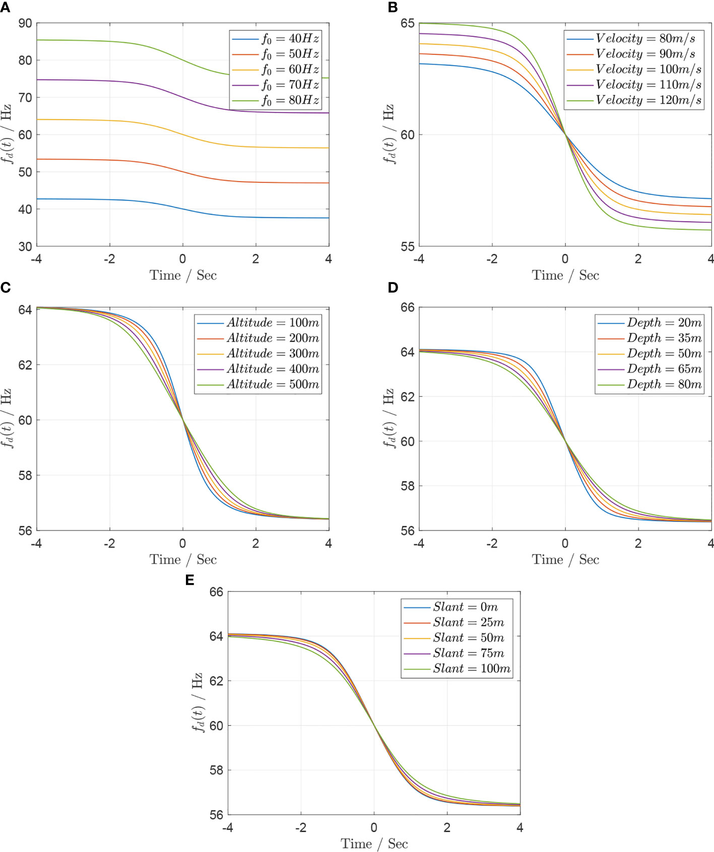
Figure 4 (A) Doppler shift curve f_d (t) versus frequency f₀ ∈ [30, 70] Hz every 10 Hz, assuming v = 100 m/s, h = 300 m, d = 50 m, and wmin = 50 m. (B) Doppler shift curve f_d (t) versus frequency v ∈ [80, 120] m/s every 10 m/s, assuming f₀ = 60 m/s, h = 300 m, d = 50 m, and wmin = 50 m. (C) Doppler shift curve f_d (t) versus frequency h ∈ [100, 500] m every 100 m, assuming f₀ = 60 m/s, v = 100 m/s, d = 50 m, and wmin = 50 m. (D) Doppler shift curve f_d (t) versus frequency d ∈ [20, 80] m every 15 m, assuming f₀ = 60 m/s, v = 100 m/s, h = 300 m, and wmin = 50 m. (E) Doppler shift curve f_d (t) versus frequency wmin ∈ [0, 100] m every 25 m, assuming f₀ = 60 m/s, v = 100 m/s, h = 300 m, and d = 50 m.

For each value of f₀ ranging from 40 to 80 Hz at an increment of 10 Hz, Figure 4A shows that the Doppler frequency f_d(t) translates along the positive direction of the f_d axis with the increase of thez source frequency f₀ .

For each value of v ranging from 80 to 120 m/s at an increment of 10 m/s, Figure 4B shows that the maximum of the frequency shift |f_d(t)−f₀| is relative with the velocity v . At the same time t , the greater the velocity is, the greater the frequency shift and its gradient are.

For each value of h ranging from 100 to 500 m at an increment of 100 m, this is illustrated in Figure 4C. For each value of d ranging from 20 to 80 m at an increment of 15 m, this is depicted in Figure 4D. For each value of w_min  ranging from 0 to 100 m at an increment of 25 m, this is presented in Figure 4E. Figures 4C–E– show that the altitude h , the depth d , and the minimum slant w_min  can affect the gradient of the Doppler frequency f_d(t) .

2.3 Estimation of flight parameters

Assuming that the sound velocity c_a and c_w in air and water, the hydrophone depth d , and its received Doppler frequency f_d(t) are known, the section proposes a solution to estimate the sound source parameters, i.e., f₀ , v , h and w_min  , using a single hydrophone.

Submitting Eq. (4) into Eq. (13), there exists

$\begin{array}{ll}{f}_d\left(t\right)=f_0{\left[1-\frac{v^{2}tcos {\beta }_T\left(t\right)}{c_w\sqrt{v^2{t}^2+w_{min }}}\right]}^{-1}.& (14)\end{array}$

The velocity v and constant frequency f₀ of source can be obtained, respectively, as follows:

$$v=c_w\frac{f_d\left(-\infty \right)-f_d\left(+\infty \right)}{f_d\left(-\infty \right)+f_d\left(+\infty \right)},$$

$\begin{array}{ll}{f}_0=2\frac{f_d\left(-\infty \right)f_d\left(+\infty \right)}{f_d\left(-\infty \right)+f_d\left(+\infty \right)}.& (15)\end{array}$

The first- and second-order derivative of f_d(t) is derived in Appendix A. The four flight parameters {h,w_min ,β_T(t)}{h,w_min ,β_T(t)} are obtained by solving a set of equations as follows:

$\begin{array}{ll}\frac{d{f}_d\left(t\right)}{dt}{|}_{t={\tau }_{\text{min }}}=f_d{}^{\text{'}}\left(f_0,v,h,w_{\text{min }}\right)=f_d{}^{\text{'}}\left({\tau }_{\text{min }}\right),& (16)\end{array}$

and

$\begin{array}{ll}\frac{d^2{f}_d\left(t\right)}{d{t}^2}{|}_{t={\tau }_{\pm 1}}=f_d{}^{"}\left(f_0,v,h,w_{\text{min }}\right).& (17)\end{array}$

Assume that the source with f₀=68Hz and v=123m/s flies along a straight line at h=200 m and the shortest projection w_min  between H and S^′ is 30 m. The time–frequency curve of the signal received by the hydrophone with a depth of 50 m is shown in Figure 5.

FIGURE 5

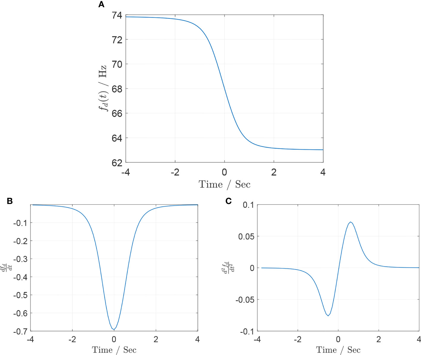
Figure 5 (A) Doppler shift curve f_d (t), assuming f₀ = 68 m/s, v = 123 m/s, h = 200 m, d = 50 m, and wmin = 30. (B) Doppler shift curve f_d (t), assuming f₀ = 68 m/s, v = 123 m/s, h = 150 m, d = 20 m, and wmin = 30. (C) Doppler shift curve f_d (t), assuming f₀ = 68 m/s, v = 123 m/s, h = 150 m, d = 20 m, and wmin = 30.

FIGURE 6

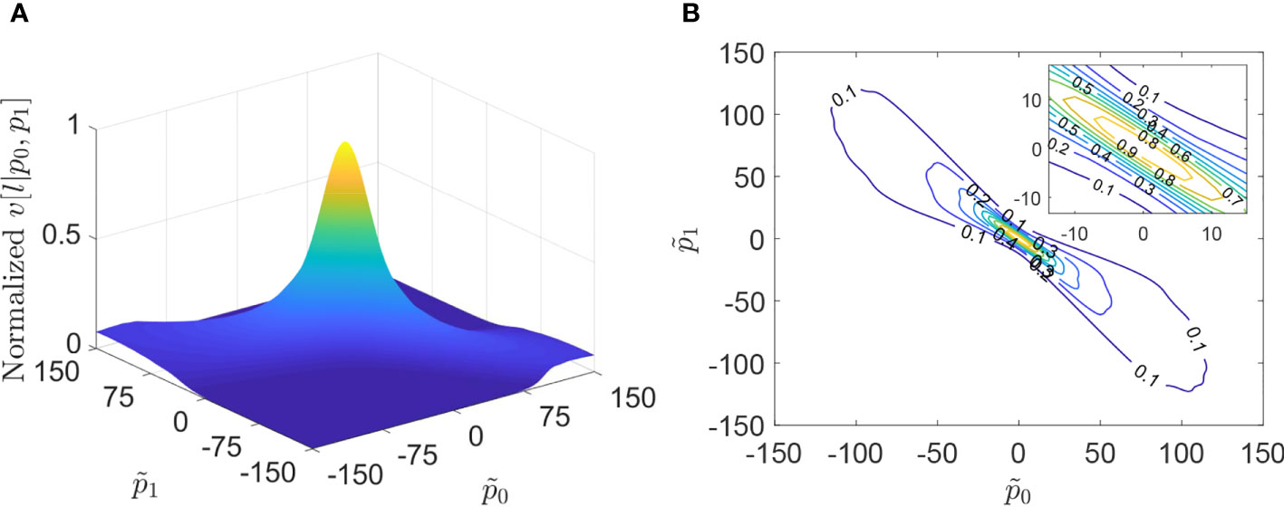
Figure 6 Accumulation power v [l|p˜n] versus p˜n with the two coefficients at l = 1,200. (A) Normalized surface and (B) contour map.

FIGURE 7

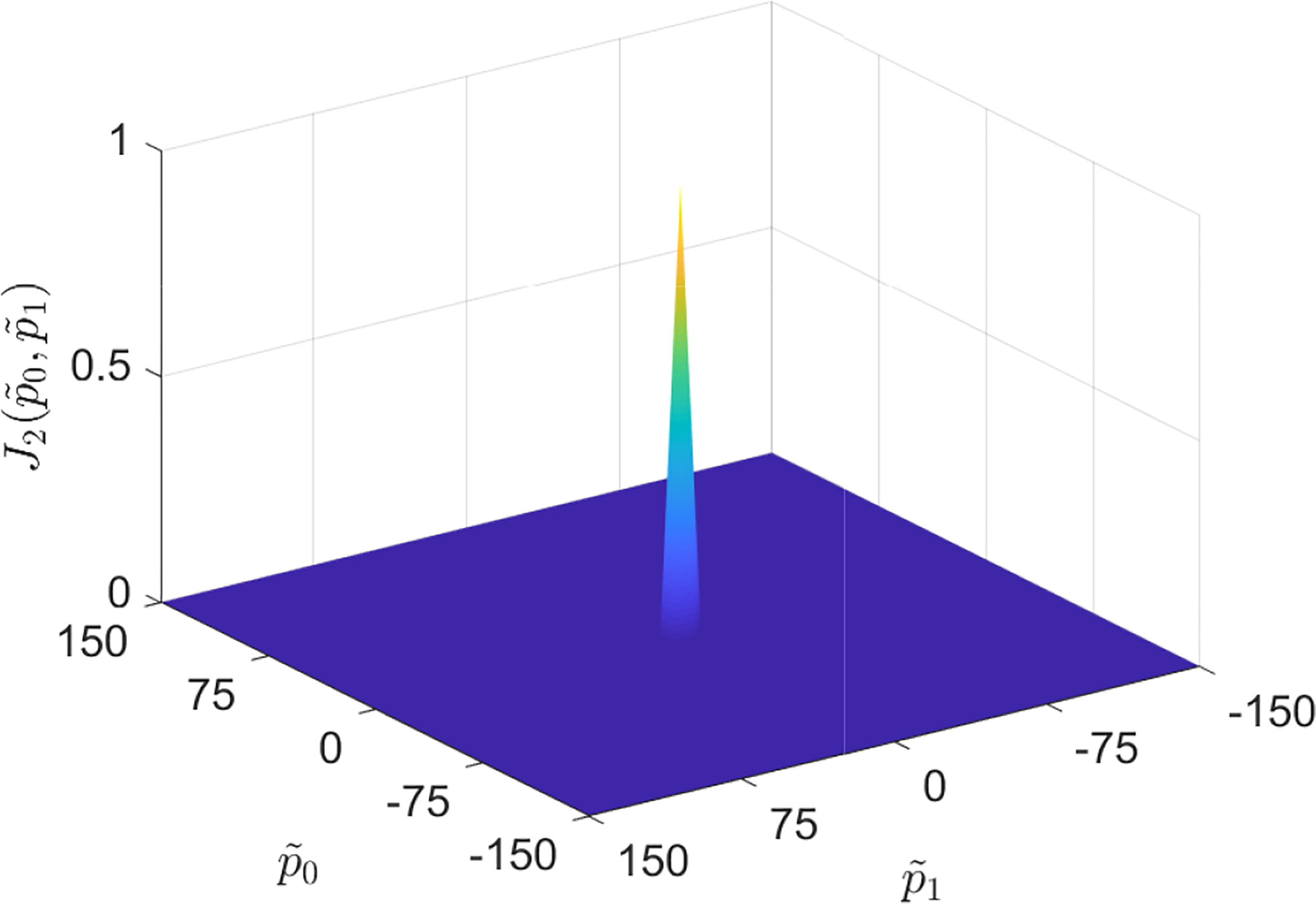
Figure 7 Normalized surface of J₂[ν(˜pu)] with U = 1 versus coefficients p˜_u ∈ [−150, 150].

Figure 5 shows that f_d(−∞) and f_d(+∞) can be approximated as f_d=73.8Hz at t=−4 s and f_d=63.4Hz at t=4 s, respectively. According to Eq. 15, v and f₀ , respectively, is given by

$$v=c_w\frac{f_d\left(-4\right)-f_d\left(+4\right)}{f_d\left(-4\right)+f_d\left(+4\right)},$$

$\begin{array}{ll}{f}_0=2\frac{f_d\left(-4\right)f_d\left(+4\right)}{f_d\left(-4\right)+f_d\left(+4\right)}.& (18)\end{array}$

Next, we solve the following equations to obtain h , w_min  , and β_T(t) at the moment t

$$f_d{}^{\text{'}}\left(0\right)=-6.921,$$

$$f_d{}^{"}\left(-0.5\right)=-7.614,$$

$\begin{array}{ll}{f}_d{}^{"}\left(0.6\right)=7.253.& (19)\end{array}$

3 Time–frequency analysis method

Under strong noise conditions, most traditional methods are not able to ensure the robustness and accuracy of time–frequency analysis simultaneously. Therefore, this section proposes a robust time–frequency analysis algorithm using a memory-dependent derivative.

3.1 The proposed algorithm

According to the theory of Ville, an analytic signal x∈ℂ^L with the time-varying IF can be given by

$\begin{array}{ll}x\left[l\right]=a{e}^{i{\displaystyle {\sum }_{m=0}^l\phi \left[m\right]}},& (20)\end{array}$

where a∈ℝ₊ and φ[m] is the amplitude and IF, respectively, and $i=\sqrt{-1}$. It should be noted that the FM signal may have a wide spectrum band since φ[m] can vary in a wide range. According to the Weierstrass approximation theorem, any continuous function in a closed and bounded interval can be uniformly approximated by a polynomial to any degree of accuracy. so φ[m] can be expanded to U -order (UłeqL−1) Taylor series at the moment m=0 , i.e.,

$\begin{array}{ll}\phi \left[m\right]=\sum _{u=0}^U\frac{{\phi }^{\left(u\right)}\left[0\right]}{u!}{\left(\frac{m}{f_s}\right)}^u+R_u\left[{\left(\frac{m}{f_s}\right)}^{u+1}\right],& (21)\end{array}$

where f_s is sample frequency, φ^(u)[0] is the u− th order difference coefficient about φ[0] , and R_u(m) is the Maclaurin remainder. There exists R_u(m)=0 when U=L−1 . Additionally, the maximum order U is related to the approximation accuracy to FM function. Specifically, U=0 for the continuous wave and U=1 for the linear FM signal. Now, by inserting Eq. (21), omitting Maclaurin remainder R_u(m) , into Eq. (20), the reformulated formula is listed as follows:

$\begin{array}{ll}x\left[l\right]=a{e}^{i{\displaystyle {\sum }_{m=0}^l{\displaystyle {\sum }_{u=0}^U{p}_u{\left(\frac{m}{f_s}\right)}^u}}},& (22)\end{array}$

where $p_u=\frac{{\phi }^{\left(u\right)}\left[0\right]}{u!}$ is the coefficient of the u -th power term. In Eq. (22), $e^{i{p}_0\frac{m}{f_s}}$ and $e^{i{\displaystyle {\sum }_{m=0}^l{\displaystyle {\sum }_{u=0}^U{p}_u{\left(\frac{m}{f_s}ight\right)}^u}}}$ is named as harmonic component and modulated element, respectively. Therefore, given a set of estimated parameters, a time–frequency estimation result is capable of producing a highly accurate approximation to a wide range of signals whose IF trajectories can be any continuous function of time. The goal of φ[m] estimation in Eq. (20) is transformed to obtain p_u in Eq. (22) since IF can be recovered from its Taylor series. In the signal estimation field, noise has always been considered as a serious cause of error. Although the most common noise can be modeled by well-known Gaussian distributions, some observed signals experience many types of i.i.d. noise with unknown distribution, for instance, underwater acoustic noise, low-frequency atmospheric noise, and other types of man-made noise (Liu et al., 2018). The signal x is corrupted by the i.i.d. noise with unknown distribution z∈ℂ^L ; then, there is an observed signal y  (Kozick and Sadler, 2000), i.e.,

$\begin{array}{ll}y\left[l\right]=x\left[l\right]+z\left[l\right].& (23)\end{array}$

Currently, there exists a class of i.i.d. noise, called symmetric α -stable (SαS ) noise, that can be used to model various types of real noise. The different noise statistical characteristics can be represented by changing parameters, where the characteristic exponent α controls the heaviness of the tails of the density function and the dispersion parameter γ determines the spread of the density around its location parameter. Thus, the probability density function of SαS gives a much better approximation to the i.i.d. noise with various distribution types.

These conventional methods can be considered as the maximum likelihood estimates resulting from corresponding minimization problems for Gaussian the noise environment. Thus, they are very sensitive to the i.i.d. noise with unknown distribution, and their robustness against a model mismatch is not ensured. In such cases, these methods under the Gaussian assumption, e.g., parametric time–frequency analysis, may exhibit a serious performance degradation for the i.i.d. noise with arbitrary distribution. The choice of a more robust solution that can be used for various i.i.d. noises is thus salutary.

A fundamental issue discussed in this paper is the question of how to improve the resolution and robustness of the time–frequency estimation result in the i.i.d. noise with arbitrary distribution. The need for robustness and high resolution in signal analysis is self-evident, yet, at the present time, the traditional assessment of such properties remains largely ad hoc. The goal has been to develop a theory and techniques for a robust and high-resolution time–frequency estimation.

3.2 Power of phase difference accumulation

The phase difference is a common tool used in polynomial phase estimation, and it is performed by multiplying each moment with a kernel function element-wise (Vucijak and Saranovac, 2010). If FM is approximated by the U -th order Taylor series in Eq. (22) and the selected kernel function is also the U -th order Taylor series with the estimated ${\widehat{p}}_u$,

$\begin{array}{ll}h\left[l|{\widehat{p}}_u\right]=e^{{}^{-i{\displaystyle {\sum }_{m=0}^l{\displaystyle {\sum }_{u=0}^U{\widehat{p}}_u{\left(\frac{m}{f_s}\right)}^u}}}},& (24)\end{array}$

so the phase difference between x and h is given by

$\begin{array}{ll}r\left[l|{\tilde{p}}_u\right]=x\left[l|p_u\right]h\left[l|{\widehat{p}}_u\right]=a{e}^{ii{\displaystyle {\sum }_{m=0}^l{\displaystyle {\sum }_{u=0}^U{\tilde{p}}_u{\left(\frac{m}{f_s}\right)}^u}}},& (25)\end{array}$

where ${\tilde{p}}_u=p_u-{\widehat{p}}_u$ is the coefficient error, and $\varphi [m|{\tilde{p}}_u]=\sum _{u=0}^U{\tilde{p}}_u{\left(\frac{m}{f_s}\right)}^u$ is defined as the IF error. As p_u is a fixed unknown value, r has also been parameterized with ${\tilde{p}}_u$ to simplify the entire expression.

Coherence accumulation to phase difference can improve the SNR, which has obtained successful applications (Vucijak and Saranovac, 2010; Wang et al., 2017). For i.i.d. noise with arbitrary distribution, the averaging value of coherence accumulation will fluctuate slightly; however, the coherence accumulation of phase difference in Eq. (25) will keep increasing as time increases, especially when ${\tilde{p}}_u$ approximates to zero. Inspired by this fundamental rule, a new cost function is constructed to find the optimal solution for all coefficients ${\tilde{p}}_u$.

We define the accumulation power of phase difference accumulation (APP) by removing the average value as

$\begin{array}{ll} v [l|{\tilde{p}}_u ]= \frac{1}{l} \sum _{m=0}^l \left\{ c\left[m\left|{\tilde{p}}_u\left] - c_M \right[m\right|{\tilde{p}}_u \right] \right\} \left\{ c\left[m\left|{\tilde{p}}_u \left] - c_M \right[m\right|{\tilde{p}}_u\right] \right\}{!}^{*} , & (26)\end{array}$

where * represents the complex conjugation, and

$\begin{array}{ll}\begin{array}{l}c\left[m\left|{\tilde{p}}_u\left]=\sum _{n=0}^{m}r\right[n\right|{\tilde{p}}_u\right],\hfill \\ c_M\left[m\left|{\tilde{p}}_u\left]=\frac{1}{m}\sum _{n=0}^{m}c\right[n\right|{\tilde{p}}_u\right],\hfill \end{array}& (27)\end{array}$

are the phase accumulation of $r[m|{\tilde{p}}_u]$ and the average of $c[m|{\tilde{p}}_u]$ over the first m≤l sample numbers, respectively. Obviously, $v\left[l|{\tilde{p}}_u\right]$ is the accumulation power of phase accumulation $r[m|{\tilde{p}}_u]$ over the interval [0,l] . THEOREM 1. The power $v\left[l|{\tilde{p}}_u\right]$ versus $\left|{\tilde{p}}_u\right|$ is the monotone function.

PROOF. We have provided the proof in the Appendix section. In Eq. (26), $\frac{dv[l|{\tilde{p}}_u]}{d{\tilde{p}}_u}\ge 0$ holds for ${\tilde{p}}_u\ge 0$ and $\frac{dv[l|{\tilde{p}}_u]}{d{\tilde{p}}_u}\le 0$ holds for ${\tilde{p}}_u\le 0$, so the maximal value of $v\left[l|{\tilde{p}}_u\right]$ will be obtained at ${\tilde{p}}_u=0$.

An example will be exhibited with the sampling frequency f_s=1,200 H and the sample number L=1,200 , the order number U=1 , and the coefficient ${\tilde{p}}_u\in \left[-150,150\right]$ for the power $v\left[l|{\tilde{p}}_u\right]$. Without loss of generality, the mesh plot of $v\left[l|{\tilde{p}}_u\right]$ versus coefficient ${\tilde{p}}_u$ at l=1,200 is demonstrated in Figure 6A, and the contour curve of $v\left[l|{\tilde{p}}_u\right]$ is shown in Figure 6B. It shows that $v\left[l|{\tilde{p}}_u\right]$ increases monotonically as coefficient ${\tilde{p}}_u$ tends to zero. Specifically, the maximum value of $v\left[l|{\tilde{p}}_u\right]$ lies at $\stackrel{�}{i}lde{p}_u=0$.

Theorems 1 and Figure 6 demonstrate that the power $v[l|{\tilde{p}}_u]$ at certain moment l is a monotonic function of $\left|{\tilde{p}}_u\right|$ and can obtain the maximum at $\left|{\tilde{p}}_u\right|=0$ if the FM signal and h are coherent. Since $v[l|{\tilde{p}}_u]$ is a positive time series as l , different types of norm, like ℓ₁ -norm, ℓ₂ -norm, and ℓ_q -norm, can be used to measure the size of $v[l|{\tilde{p}}_u]$. From a statistical perspective, ℓ₂ -norm is suitable for Gaussian noise and ℓ₁ -norm is robust to outliers. Since $v[l|{\tilde{p}}_u]$ could be corrupted by SαS noise with impulses and the estimated IF can be determined by maximizing $v[l|{\tilde{p}}_u]$ at any moment, ℓ₁ - norm will be chosen. Therefore, the problem of coefficient ${\tilde{p}}_u$ estimation can be readily solved by ℓ₁ -norm maximization as follows:

$\begin{array}{ll}\underset{{\widehat{p}}_u}{\max }\Vert v[l|{\tilde{p}}_u]{\Vert }_{1}s.t.{\tilde{p}}_u=p_u-{\widehat{p}}_u.& (28)\end{array}$

Moreover, Theorem 1 guarantees that the accurate coefficient. is available in the continuous domain, and the previous work in time–frequency estimation is fundamentally limited by the Heisenberg–Gabor inequality for a better resolution. The estimated IF can be approximated as $\widehat{\varphi }[m|{\widehat{p}}_u]={\displaystyle {\sum }_{u=0}^U{\widehat{p}}_u{\left(\frac{m}{f_s}\right)}^u}$.

3.3 IF estimation based on multiple log-sum

Under the condition of short window size L or high noise power, the estimated IF trajectory with ℓ₁ - norm shows poor accuracy and is easily interrupted by the accumulation of noises, although the maximal value in (28) is still obtained at the true p_u from the statistical perspective. In view of the nonlinear amplification for DOA estimation in Wang et al. (2008) and Wang and Kay (2010), the multiple logarithmic sum (MLS) is proposed to achieve the sharper peak for target IF and deeper null for non-target area, which also improves the accurate and robust performance for IF estimation.

Log-sum function has often been used to solve for maximization and is shown to be more convex and smoother than the ℓ₁ -norm (Zhang et al., 2019; Qiao et al., 2020), and this function can exhibit nonlinear amplification in some fixed intervals. Alternating convexity-promoting functions such as log-sum function can be used to replace the ℓ₁ -norm, and a surrogate function with a sharper peak for target frequency and deeper null for side lobes is achieved. Thus, we consider the use of the log-sum function to improve the convexity of the objective function. Replacing the ℓ₁ -norm in Eq. (28) with the multiple log-sum function over the entire sample number L will result in

$\begin{array}{ll}\underset{{\widehat{p}}_u}{\max }{J}_1\left({\tilde{p}}_u\right)={\displaystyle \sum _{l=0}^{L-1}\text{log }\left\{v[l\mid {\tilde{p}}_u]+1\right\}s.t.{\tilde{p}}_u=p_u-{\widehat{p}}_u.}& (29)\end{array}$

where “1” is added to ensure that $\text{log }\left\{v[l|{\tilde{p}}_u]+1\right\}$ is non-negative, and it does n’t change the location of the optimal solution. $J_1\left({\tilde{p}}_u\right)$ versus $\left|{\tilde{p}}_u\right|$ is also monotonic since log  is a monotonic function and $v[l|{\tilde{p}}_u]$ versus $\left|{\tilde{p}}_u\right|$ is a monotonic decreasing function as proved in Theorem 1. $J_1\left({\tilde{p}}_u\right)$ in Eq. (29) is rewritten as follows:

$\begin{array}{ll}{J}_1\left({\tilde{p}}_u\right)=\text{log}{\displaystyle \coprod _{l=0}^{L-1}\left\{v[l\mid {\tilde{p}}_u]+1\right\}=\text{log }\nu \left({\tilde{p}}_u\right),}& (30)\end{array}$

so $J_1\left({\tilde{p}}_u\right)$ can also be considered as the function of $\nu \left({\tilde{p}}_u\right)$ and rewritten as $J_1\left[\nu \left({\tilde{p}}_u\right)\right]$. Hence, for $J_1\left[\nu \left({\tilde{p}}_u\right)\right]$, the accumulation of the frequency domain is transformed into the integral of power in the logarithm space. Benefiting from the monotonicity of $\nu \left({\tilde{p}}_u\right)$ versus $v(t|{\tilde{p}}_n)$as proved in Theorem 2, the sum of $J_1\left[\nu \left({\tilde{p}}_u\right)\right]$ over $\nu \left({\tilde{p}}_u\right)$ can significantly amplify the power $v(t|{\tilde{p}}_n)$ in a non-linear way. Without loss of generality, only the accumulation over the non-positive interval of ${\tilde{p}}_u$ is considered since $v[l|{\tilde{p}}_u]$ is an even function. According to Theorems 1 and 6, the power $v[l|{\tilde{p}}_u]$ tends to zero when ${\tilde{p}}_u\to 0$. Thus, the lower integral limit can be obtained as follows:

$\begin{array}{ll}\underset{{\tilde{p}}_u\to -\infty }{\lim }\text{log }\nu \left({\tilde{p}}_u\right)=\underset{{\tilde{p}}_u\to -\infty }{\lim }\text{log}{\displaystyle \prod _{l=0}^{L-1}\left\{v[l\mid {\tilde{p}}_u]+1\right\}=C_0.}& (31)\end{array}$

Consequently, the variable upper limit integral of $J_1\left[\nu \left({\tilde{p}}_u\right)\right]$ over the continuous domain $\nu \left({\tilde{p}}_u\right)$ is given by

$\begin{array}{ll}{J}_2\left[\nu \left({\tilde{p}}_u\right)\right]=\underset{C_0}{\overset{\nu \left({\tilde{p}}_u\right)}{\int }}\left(\text{log }\kappa +1\right)d\kappa =\nu \left({\tilde{p}}_u\right)\text{log }\nu \left({\tilde{p}}_u\right)+C_1,& (32)\end{array}$

where a fixed constant “1” added in the integral is added to obtain a simple analytical solution. Because the linear accumulation of $J_2\left[\nu \left({\tilde{p}}_u\right)\right]$ with the constant term does not change the extreme value point, it does not affect the final solution coefficient ${\tilde{p}}_u$. Besides that, Eq. (32) with respect to $\nu \left({\tilde{p}}_u\right)$ is convex according to Chapter 3 in Boyd et al. (2004).

THEOREM 2. $J_2\left[\nu \left({\tilde{p}}_u\right)\right]$ versus $\left|{\tilde{p}}_u\right|$is monotone decreasing.

PROOF. According to the chain rule of derivation, the first-order derivative of $J_2\left[\nu \left({\tilde{p}}_u\right)\right]$ about $\left|{\tilde{p}}_u\right|$ is given by

$$\frac{d{J}_2\left[\nu \left({\tilde{p}}_u\right)\right]}{d\left|{\tilde{p}}_u\right|}=\frac{d{J}_2}{d\nu }\sum _{l=0}^{L-1}\left(\frac{d\nu }{dv\left[l\right]}\frac{dv\left[l|{\tilde{p}}_u\right]}{d\left|{\tilde{p}}_u\right|}\right).$$

Firstly, it follows from Theorem 1 that $v\left[l|{\tilde{p}}_u\right]$ is a monotonically decreasing function of $\left|{\tilde{p}}_u\right|$, and there exists $\frac{dv\left[l|{\tilde{p}}_u\right]}{d\left|{\tilde{p}}_u\right|}\le 0$.

Secondly, the first-order derivative of the composite function ν{v[l]} about v[l] from Eq. (30) is given by

$$\frac{d\nu \left\{v\left[l\right]\right\}}{dv\left[l\right]}={\left\{\prod _{l=0}^{L-1}\left\{v[l|{\tilde{p}}_u]+1\right\}\right\}}^{"}{}_{v\left[l\right]}=\sum _{l=0}^{L-1}\prod _k\left\{v[k|{\tilde{p}}_u]+1\right\},$$

where k∈{0,L−1}​\​{l} . $\frac{d\nu \left\{v\left[l\right]\right\}}{dv\left[l\right]}$is non-negative since $v[l|{\tilde{p}}_u]$ is non-negative. Thus, it indicates that ν bracev[l]} versus v[l] is monotonically increasing. Thirdly, the first-order derivative of J₂(ν) is calculated as follows:

$$\frac{d{J}_2\left[\nu \right]}{d\nu }=\frac{1}{\nu \left({\tilde{p}}_u\right)}+1,$$

which is positive since $\nu \left({\tilde{p}}_u\right)\ge 0$. Thus, J₂(ν) is monotonically increasing.

To summarize the above-mentioned points, in the case of $\frac{d\varphi }{dt}⋚$, the first-order derivative of $J_2\left[\nu \left({\tilde{p}}_u\right)\right]$ about $\left|{\tilde{p}}_u\right|$ is non-positive, i.e.,

$$\frac{d{J}_2\left[\nu \left({\tilde{p}}_u\right)\right]}{d\left|{\tilde{p}}_u\right|}\le 0.$$

Therefore, it is proven.

After the nonlinear amplification with convexity-preserving operation and the accumulation in the frequency domain, $J_2\left[\nu \left({\tilde{p}}_u\right)\right]$ versus ${\tilde{p}}_u$ has a sharper peak and a deeper null level than $J_1\left[\nu \left({\tilde{p}}_u\right)\right]$ in (29). $J_2\left[\nu \left({\tilde{p}}_u\right)\right]$ with two coefficients is depicted in Figure 7, and the same simulation condition as in Figure 6 is kept. The deep null level of $J_2\left[\nu \left({\tilde{p}}_u\right)\right]$ at the unmatched phase is beneficial to find the optimal coefficients and suppress the i.i.d. noise. Since $J_2\left[\nu \left({\tilde{p}}_u\right)\right]$ is convex, any gradient algorithm can be used to solve this maximization problem.

In summary, the time–frequency estimation by the APP-MLS algorithm can be converted into the maximization problem as follows:

$\begin{array}{ll}\underset{{\widehat{p}}_u}{\max }{J}_3\left({\tilde{p}}_u\right)=\nu \left({\tilde{p}}_u\right)\text{log }\nu \left({\tilde{p}}_u\right)s.t.{\tilde{p}}_u=p_u-{\widehat{p}}_u.& (33)\end{array}$

We propose the APP-MLS algorithm to find the optimal solution for (37), and the basic idea of the IF estimation by the APP-MLS algorithm is to determine the coefficients ${\widehat{p}}_u$ of polynomial kernel to estimate the time–frequency trajectory. The details will be introduced in the next section. Due to the convexity of $J_3\left({\tilde{p}}_u\right)$, any gradient algorithm can be used to solve this maximization problem. In this paper, the optimization solution ${\widehat{p}}_n$ is obtained by maximizing Eq. (33) by the AdaBelief method, which is more efficient for the parameter tuning process. The intuition for AdaBelief is to adapt the step size according to the “belief” in the current gradient direction. This method uses the exponential moving average of the noisy gradient as the prediction of the gradient at the next time step; if the observed gradient greatly deviates from the prediction, we distrust the current observation and take a small step; if the observed gradient is close to the prediction, we trust it and take a large step. After localizing the ${\widehat{p}}_u$ in one time interval, the estimated time–frequency trajectory $\widehat{\phi }[m|{\widehat{p}}_u]={\displaystyle {\sum }_{u=0}^U{\widehat{p}}_u{\left(\frac{m}{f_s}\right)}^u}$ can be obtained.

In practical application, the whole observed data will be partitioned into many overlapped slides with the window size τ and the overlap size S between two close windows; then, the number K of slides can be obtained. The polynomial order U and the initial coefficient ${\widehat{p}}_u$ are given according to the rough character of the signal. In every slide, therein included are the following steps: firstly, the phase difference between the truncated signal and the kernel function is calculated, and its accumulated power can be obtained. Furthermore, by maximizing the multiple log-sum function with the AdaBelief algorithm, the estimated coefficient ${\widehat{p}}_u$ can be obtained after several iterations. Finally, the estimated IF trajectory can be obtained within the overlap size S . The detailed procedure is illustrated in Figure 8.

FIGURE 8

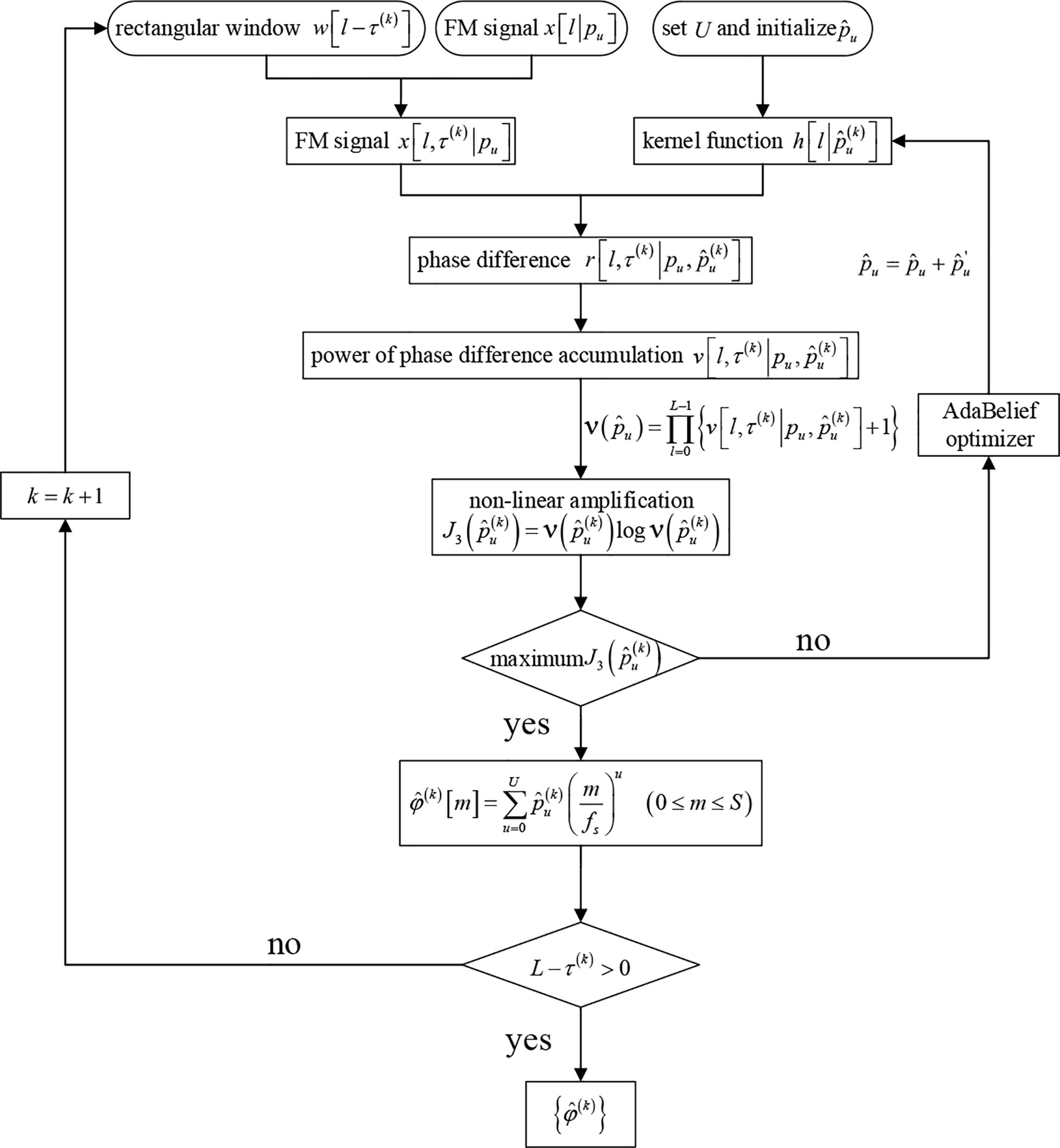
Figure 8 Time–frequency estimation based on APP-MLS.

During the application of the APP-MLS algorithm, the estimation accuracy of the IF trajectory depends on the order U , the window size W , and the overlap size S (0​≤​S​<​W ). Specifically, as the order U increases, the Taylor series can approximate the estimated frequency function φ[m] with a high accuracy within a fixed window size W . The longer window size W leads to larger deviations from the true IF trajectory at a fixed order U , especially at the window end. The window size W also affects the robustness of the algorithm, i.e., the longer the window size, the better robustness to suppress noise; it should not be too short in practical application. Additionally, the higher-order U and longer window size W will increase the computation complexity, and their choice should be considered carefully.

4 Example

The 120-s aircraft noise data are used to validate the efficiency of the estimation model of flight parameters. These data were measured in an experiment where an aircraft traveled along a straight path at a constant speed. The speed of sound in air and seawater was 340 and 1,520 m/s, respectively. A hydrophone is placed at a depth of 90 m in the ocean, and its output is sampled at 44.1 kHz for 2 min. To reduce the computational burden, the data herein are downsampled to 1,200 Hz.

The Acoustical Society of America provided a piece of audio data¹, where a hydrophone is placed at a depth of 90m in the ocean and records the underwater acoustic data from a turboprop aircraft with a constant frequency of 68 Hz flying straightly over the hydrophone at a fixed altitude. The sampling rate is 44.1 kHz, and the recorded time is 120 s, as shown in Figure 9. As the aircraft approximates and leaves the overhead of the hydrophone, the relative Doppler of the received acoustic signal has an apparent and quick change, and the IF trajectory can determine the flying parameters of the aircraft. The detailed analysis and principle can be referred to Urick R J (Urick et al, 1972) and the accurate estimation of the IF trajectory is very important. According to Tre DiPassio’s 2019 Challenge Problem Solution, the original propeller frequency is estimated when the plane is directly overhead the hydrophone at a timestamp denoted as 54 s. To better show the estimated IF results for radiated noise, we intercepted the data from 49 to 59 s when the aircraft is nearly over the hydrophone.

FIGURE 9

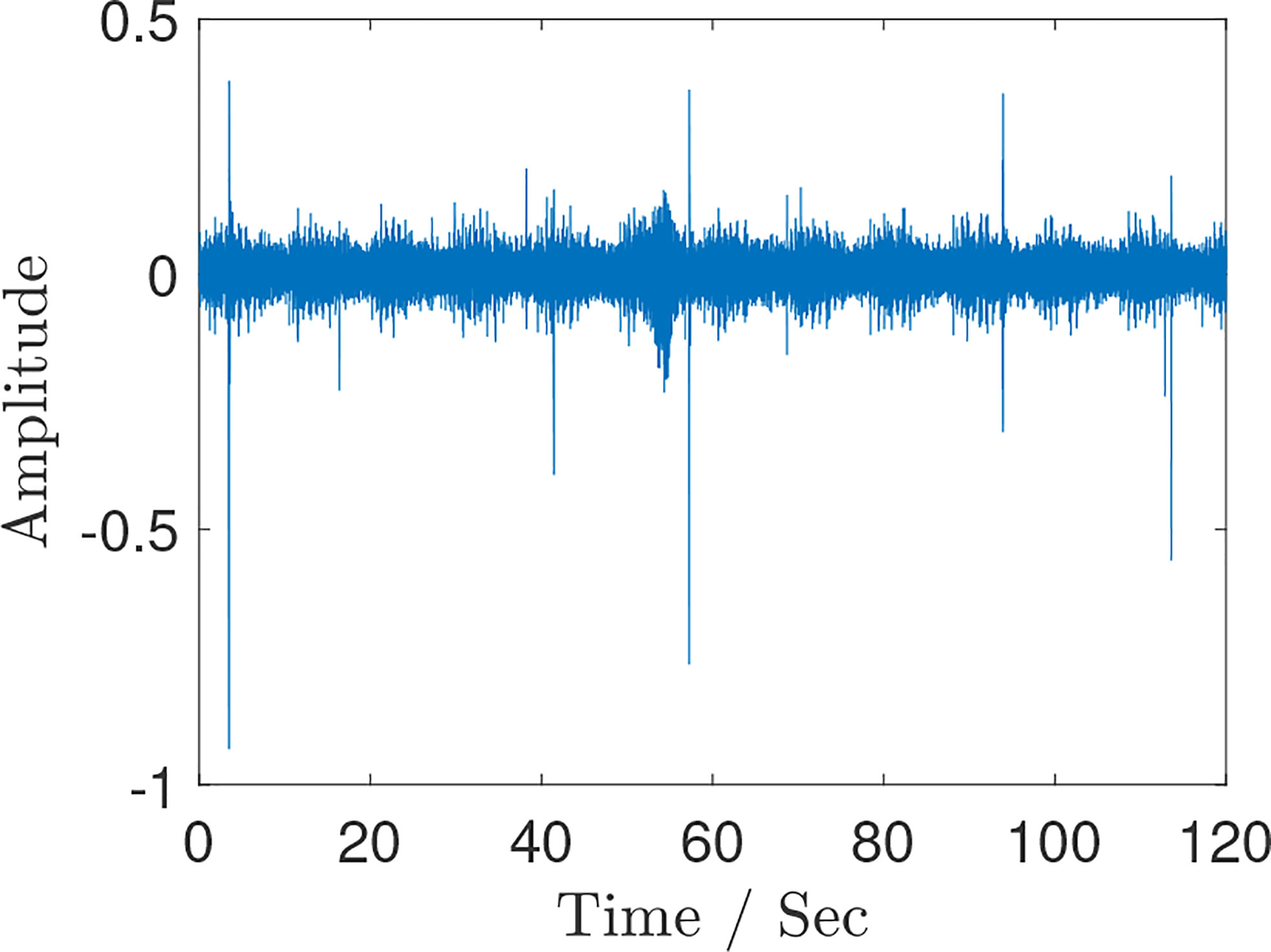
Figure 9 Helicopter waveform in each frame of the given audio file.

The maximum frequency bin of each frame is used to estimate the fundamental frequency present in that frame. Figure 10 shows these estimates as well as the amplitude computed in each frame. The majority of the audio solely contain underwater noise. However, at around 54 s, a few seconds of a plane flying overhead can be heard when listening to the file. The presence of the plane is shown in the highlighted section of Figure 10. There is a spike in the amplitude above the noise floor, paired with a more defined instantaneous frequency track. Figure 11 shows only the frames where the plane flying overhead is audible commensurate to the amplitude spike in Figure 10.

FIGURE 10

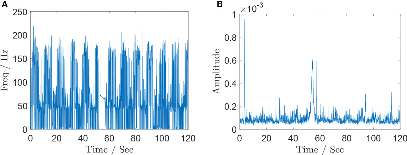
Figure 10 Instantaneous frequency estimation results for the aircraft acoustic data recorded by hydrophone with (A) the estimated fundamental frequency in each frame of the given audio file and (B) the estimated amplitude in each frame of the given audio file.

FIGURE 11

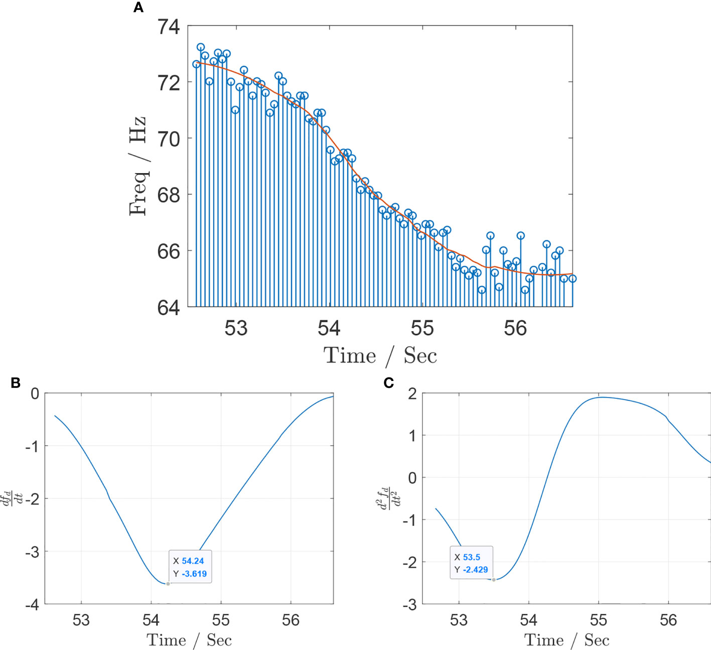
Figure 11 Instantaneous frequency estimation results for the aircraft acoustic data recorded by hydrophone with (A) raw and smoothed frequency track at the hydrophone position. (B) First-order derivative of the Doppler shift curve f_d (t). (C) Second-order derivative of the Doppler shift curve f_d (t).

In order to extract instantaneous frequencies from the provided file, a short-time Fourier transform (STFT) is utilized in Figure 11. The audio is split into frames with a length of 8,192 samples per frame, windowed with an 8,192-point Hamming window. Each frame is converted to the frequency domain using the fast Fourier transform (FFT) algorithm run on the frame data. In total, 75% overlap is used between the frames, and zero padding is added such that the frequency resolution (bin size) of the FFT in each frame is approximately 0.1 Hz. Consistent with the Nyquist Theorem, the maximal frequency present in the given audio is half the sampling frequency or 22,050 Hz. Therefore, the full-scale 22,050 Hz will be represented in the number of frequency bins equal to half of the FFT length due to the redundancy added when computing the FFT. The following equation thus shows how the desired resolution is achieved:

$\begin{array}{ll}\text{Resolution}=\frac{f_s}{\text{FFTLEN}}& (34)\end{array}$

Solving Eq. (38) for the desired resolution of around 0.1 Hz in each frame shows that 53-times zero padding should be used.

The estimates from each frame in the region with audible plane motion are smoothed to create an instantaneous frequency track. This smoothing is done with a Savitzky–Golay filter. This type of filter is used to smooth sets of data points in the time domain using a least-squares fitting approach.

The estimated IF trajectory by the APP-MLS will be compared with STFT, PCT, and SST. Because of the high data sampling rate and the frequency of interest being located in the low-frequency range, the data were downsampled by 200 times. In order to estimate the IF better and compare fairly, some parameters of different methods will be set. The window size is set to W=128 , and the overlap rate is set as 75%. Moreover, the iteration number of PCT is seven, the synchronous squeeze factor of SST is 200, and the maximum order of APP-MLS is U=2 . Besides this, in Tre DiPassio’s 2019 Challenge Problem Solution², the author gives details about how to extract data from provided audio, which is given as follows: firstly, the audio is split into frames with a length of 128 samples per frame, windowed with a 128-point Hamming window. Secondly, each frame is converted to the frequency domain using the fast Fourier transform algorithm run on the frame data. Then, 75% overlap is used between the frames, and 16 times more zero padding is added such that the frequency resolution of these methods in each frame is approximately 0.1 Hz. Thirdly, the maximum frequency bin of each frame is used to estimate the fundamental frequency present in that frame. Finally, this smoothing is done with a Savitzky–Golay filter to smooth the IF curve.

Figure 12 presents the estimated results of the four methods. Although the changing trend of IF estimation by STFT can be observed as shown in Figure 12A, there exist severe fluctuations outside the interval 53–57 s when the aircraft deviates far from the head of hydrophone. Figures 12B, C show that the interference within the frequency range of interest by PCT and SST has been improved because the adaptive kernel function and the synchrosqueezing transform are used respectively. However, they are also distorted by the background noise with unknown probability distribution, and their estimated IF information is still not available effectively when the aircraft is far from the hydrophone. Benefitting from the gridless principle and nonlinear amplification, the IF trajectory yielded by APP-MLS can effectively suppress underwater acoustic noise even for low SNR. The IF result within the range of interest shown in Figure 12D is more accurate than the other three methods. The APP-MLS algorithm shows the robust IF estimation performance in the lower SNR environment, and its result is much closer to the true IF than those of the other methods.

FIGURE 12

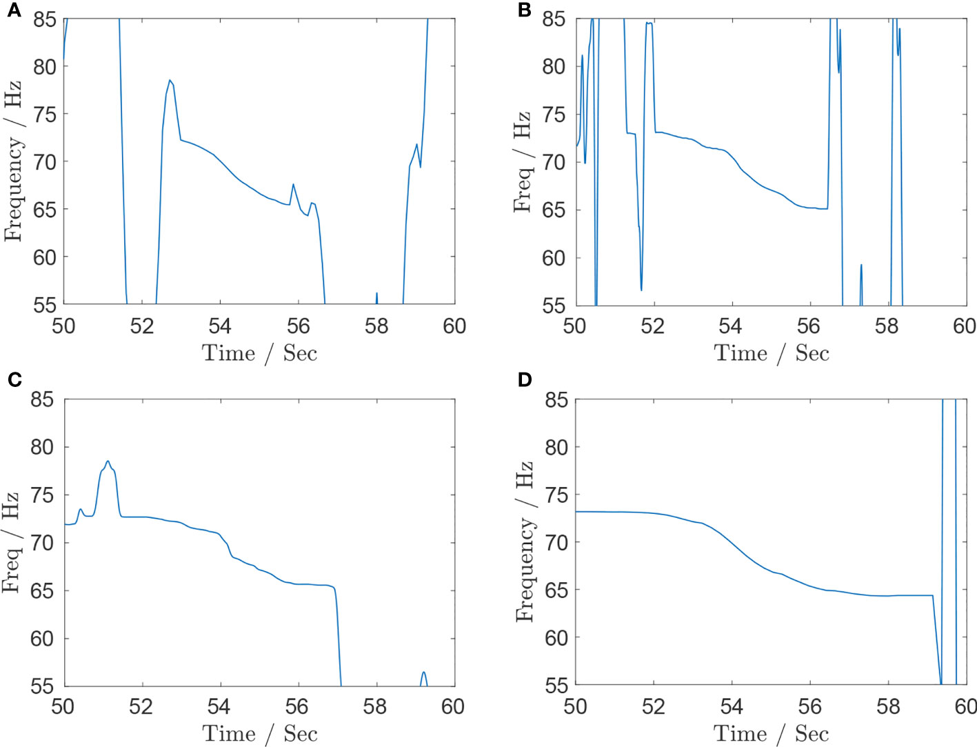
Figure 12 Instantaneous frequency estimation results for the aircraft acoustic data recorded by hydrophone with (A) STFT, (B) PCT, (C) SST, and (D) APP-MLS.

The experimental frequency values from Figure 11 range from 64.17 to 73.45 Hz, for a total range of 9.28 Hz. Substituting these values into Eq. (15) will yield as follows:

$\begin{array}{ll}\{\begin{array}{rr}\hfill f_0& \hfill =2\frac{f_d\left(-\infty \right)f_d\left(+\infty \right)}{f_d\left(-\infty \right)+f_d\left(+\infty \right)}\approx 2\times \frac{73.45\times 64.17}{73.45+64.17}=68.5 \text{Hz}\\ \hfill v& \hfill =c_w\frac{f_d\left(-\infty \right)-f_d\left(+\infty \right)}{f_d\left(-\infty \right)+f_d\left(+\infty \right)}\approx 1520\times \frac{73.45-64.17}{73.45+64.17}=101 \text{m}/\text{s}\end{array}& (35)\end{array}$

so the aircraft frequency is 68.5 Hz, and the speed of the aircraft is 101 m/s.

According to the first- and second-order derivative of f_d(t) , the rest of the two flight parameters {h,w_min } are obtained by solving a set of equations as follows:

$\begin{array}{ll}\frac{d{f}_d\left(t\right)}{dt}=f_d{}^{\text{'}}\left(f_0,v,h,w_{\text{min }}\right)=-3.619,& (36)\end{array}$

and

$\begin{array}{ll}\frac{d^2{f}_d\left(t\right)}{d{t}^2}=f_d{}^{"}\left(f_0,v,h,w_{\text{min }}\right)=-\mathrm{2.429.}& (37)\end{array}$

Then, we obtain h=150.1m and w_min =1.4m .

5 Conclusion

This paper proposes the use of both time–frequency trajectory and three-dimensional space model to estimate the flight parameters, including {f₀,v,α(t),β(t)} . This solution explores a computational approach using the geometric relationships of three-dimensional space and using the result of time–frequency estimation to create a predictive model for the instantaneous frequency observed at the hydrophone position by using Doppler effect calculations. The accuracy of this model will be evaluated via comparison with given experimental data. The model will then be used to extract the propeller frequency, speed, height, and slant of the aircraft source for a given hydrophone recording.

Data availability statement

The original contributions presented in the study are included in the article/supplementary material. Further inquiries can be directed to the corresponding author.

Author contributions

All authors listed have made a substantial, direct, and intellectual contribution to the work, and approved it for publication.

Funding

This Project are supported by the Key Laboratory of Intelligent Image Processing and Analysis(Wenzhou, China, No.2021HZSY0071) and the Key Project of Zhejiang Provincial Natural Science Foundation under Grant (No.LZ20F020004).

Conflict of interest

The authors declare that the research was conducted in the absence of any commercial or financial relationships that could be construed as a potential conflict of interest.

Publisher’s note

All claims expressed in this article are solely those of the authors and do not necessarily represent those of their affiliated organizations, or those of the publisher, the editors and the reviewers. Any product that may be evaluated in this article, or claim that may be made by its manufacturer, is not guaranteed or endorsed by the publisher.

Footnotes

1. ^ https://acousticstoday.org/iscpasp2019
2. ^ https://www.tredipassio.com/asa2019?rq=asa

References

Aksenovich T. V. (2020). “Comparison of the use of wavelet transform and short-time fourier transform for the study of geomagnetically induced current in the autotransformer neutral,” in 2020 international multi-conference on industrial engineering and modern technologies (FarEastCon). pp. 1–5. doi: 10.1109/FarEastCon50210.2020.9271210

CrossRef Full Text | Google Scholar

Aygun H., Kirmizi M., Turan O. (2022). Propeller effects on energy, exergy and sustainability parameters of a small turboprop engine. Energy 249, 123759. doi: 10.1016/j.energy.2022.123759

CrossRef Full Text | Google Scholar

Boashash B. (2015). Time-frequency signal analysis and processing: A comprehensive reference (Massachussetts, Washington, DC: Academic Press).

Google Scholar

Boyd S., Boyd S. P., Vandenberghe L. (2004). Convex optimization (University Printing House, Cambridge: Cambridge university press).

Google Scholar

Chirico G., George N., Barakos and Nicholas Bown. (2018). Propeller installation effects on turboprop aircraft acoustics. 424, 238–62. doi:10.1016/j.jsv.2018.03.003

CrossRef Full Text | Google Scholar

Fang J., Wang F., Shen Y., Li H., Blum R. S. (2016). Super-resolution compressed sensing for line spectral estimation: An iterative reweighted approach. IEEE Trans. Signal Process. 64, 4649–4662. doi: 10.1109/TSP.2016.2572041

CrossRef Full Text | Google Scholar

Kozick R. J., Sadler B. M. (2000). Maximum-likelihood array processing in non-Gaussian noise with Gaussian mixtures. IEEE Trans. Signal Process. doi: 10.1109/78.887045

CrossRef Full Text | Google Scholar

Kumar A., Prasad A. (2022). Wigner-ville distribution function in the framework of linear canonical transform. J. Pseudo Differential Operators Appl. 13, 1–17. doi: 10.1007/s11868-022-00471-w

CrossRef Full Text | Google Scholar

Liu S., Zhang Y. D., Shan T. (2018). Detection of weak astronomical signals with frequency-hopping interference suppression. Digital Signal Process. 72, 1–8. doi: 10.1016/j.dsp.2017.09.003

CrossRef Full Text | Google Scholar

Qiao C., Shi Y., Diao Y. X., Calhoun V. D., Wang Y. P. (2020). Log-sum enhanced sparse deep neural network. Neurocomputing 407, 206–220. doi: 10.1016/j.neucom.2020.04.118

CrossRef Full Text | Google Scholar

Urick R. J. (1972). Noise Signature of an Aircraft in Level Flight over a Hydrophone in the Sea[J]. J. Acoust. Soc. Am. 52 (1A), 993–999.

Google Scholar

Vandana A. R., Arokiasamy M. (2022). Comparison of radar micro doppler signature analysis using short time fourier transform and discrete wavelet packet transform. doi: 10.1007/978-981-16-9012-9_35

CrossRef Full Text | Google Scholar

Vucijak N. M., Saranovac L. V. (2010). A simple algorithm for the estimation of phase difference between two sinusoidal voltages. IEEE Trans. Instrum. Meas. 59, 3152–3158. doi: 10.1109/TIM.2010.2047155

CrossRef Full Text | Google Scholar

Wang H., Kay S. (2010). Maximum likelihood angle-doppler estimator using importance sampling. IEEE Trans. Aerospace Electronic Syst. 46, 610–622. doi: 10.1109/TAES.2010.5461644

CrossRef Full Text | Google Scholar

Wang H., Kay S., Saha S. (2008). An importance sampling maximum likelihood direction of arrival estimator. IEEE Trans. Signal Process. 56, 5082–5092. doi: 10.1109/TSP.2008.928504

CrossRef Full Text | Google Scholar

Wang P., Orlik P. V., Sadamoto K., Tsujita W., Gini F. (2017). Parameter estimation of hybrid sinusoidal fm-polynomial phase signal. IEEE Signal Process. Lett. 24, 66–70. doi: 10.1109/LSP.2016.2638436

CrossRef Full Text | Google Scholar

Zcza B., Szq A., Xian J. A., Pyh A., Xys A., Ayw A. (2021). Linear canonical wigner distribution of noisy lfm signals via variance-snr based inequalities system analysis. Optik 237, 166712. doi: 10.1016/j.ijleo.2021.166712

CrossRef Full Text | Google Scholar

Zhang W., Fu L., Liu Q. (2019). Nonconvex log-sum function-based majorization-minimization framework for seismic data reconstruction. IEEE Geosci. Remote Sens. Lett. PP 1–5, 1776–1780. doi: 10.1109/LGRS.2019.2909776

CrossRef Full Text | Google Scholar

Zhang X., Wu H., Sun H., Ying W. (2021). Multireceiver sas imagery based on monostatic conversion. IEEE J. Selected Topics Appl. Earth Observations Remote Sens. 14, 10835–10853. doi: 10.1109/JSTARS.2021.3121405

CrossRef Full Text | Google Scholar

Zhang X., Yang P., Huang P., Ying W. (2022). Wide-bandwidth signal-based multireceiver sas imagery using extended chirp scaling algorithm. IET Radar Sonar Navigation. doi: 10.1049/rsn2.12200

CrossRef Full Text | Google Scholar

Zhang X., Ying W., Yang P., Sun M. (2020). Parameter estimation of underwater impulsive noise with class b model. IET Radar Sonar Navigation. doi: 10.1049/iet-rsn.2019.0477

CrossRef Full Text | Google Scholar

Zhou C., Zhang G., Yang Z., Zhou J. (2020). A novel image registration algorithm using wavelet transform and matrix-multiply discrete fourier transform. IEEE Geosci. Remote Sens. Lett. PP 1–5, 8002605. doi: 10.1109/LGRS.2020.3031335

CrossRef Full Text | Google Scholar

Appendix.

$\begin{array}{ll}\begin{array}{l}\frac{d{f}_d}{dt}=\frac{f_0{c}_w{v}^2}{\sqrt{v^2{t}^2+w_{min }^2}}\{\frac{d{\beta }_T\left(t\right)}{dt}t\left(v^2{t}^2+w_{\min }^2\right)\sin {\beta }_T\hfill \\ -\left(2v^2{t}^2+w_{\min }^2\right)\cos {\beta }_T\left(t\right)+t\}.\end{array}& (38)\end{array}$

$\begin{array}{ll}\frac{d\beta }{dt}={(A_1+A_2-A_3+A_4{A}_5+A_3{A}_6{A}_7^{-1}-A_8{A}_9-A_{10})}^{-1}{A}_{11}.& (39)\end{array}$

where

$\begin{array}{ll}\begin{array}{l}{A}_1=\cos \beta \left(t\right)\sqrt{1-n^2\stackrel{2}{\cos }\beta \left(t\right)},\hfill \\ A_2=n^2{\left[1-n^2\stackrel{2}{\cos }\beta \left(t\right)\right]}^{-1/2}\stackrel{2}{\sin }\beta \left(t\right)\cos \beta \left(t\right),\hfill \\ A_3=2n\sin \beta \left(t\right)\cos \beta \left(t\right),\hfill \\ A_4=\cos \beta \left(t\right)\sqrt{1-n^2\stackrel{2}{\cos }\beta \left(t\right)}/\left(2dh\right),\hfill \\ A_5=d^2/\left(1-n^2\stackrel{2}{\cos }\beta \left(t\right)\right)+h^2/\stackrel{2}{\sin }\beta \left(t\right)\hfill \\ -[\left(d+h{)}^2+v^2{t}^2+w_{\min }^2\right],A_6=d^2/\left(1-n^2\stackrel{2}{\cos }\beta \left(t\right)\right)+h^2/\stackrel{2}{\sin }\beta \left(t\right)\hfill \\ -\left[{\left(d+h\right)}^2+v^2{t}^2+w_{\min }^2\right],A_7=2dh\sqrt{1-n^2\stackrel{2}{\cos }\beta \left(t\right)},A_8=\sin \beta \left(t\right)\sqrt{1-n^2\stackrel{2}{\cos }\beta \left(t\right)}/\left(2dh\right),\hfill \\ A_9=2d^2{h}^2\stackrel{2}{\sin }\beta \left(t\right)\cos \beta \left(t\right)/{\left(1-n^2\stackrel{2}{\cos }\beta \left(t\right)\right)}^2,\hfill \\ A_{10}=h\sqrt{1-n^2\stackrel{2}{\cos }\beta \left(t\right)}/\left[d\sin \beta \left(t\right)\right],\hfill \\ A_{11}=v^{2}t\sin \beta \left(t\right)\sqrt{1-n^2\stackrel{2}{\cos }\beta \left(t\right)}/\left(2dh\right),\hfill \end{array}& (40)\end{array}$

$\begin{array}{ll}\frac{d^2{f}_d}{d{t}^2}=\frac{c_w{f}_0{v}^2\left(G_1+G_2+G_3-G_4\right)}{2G_5}.& (41)\end{array}$

$\begin{array}{ll}\begin{array}{l}{G}_1=-2t\frac{d^2\beta }{d{t}^2}\sin \beta \left(t\right){(v^2{t}^2+w_{\min }^2)}^2\left[v^{2}t\cos \beta \left(t\right)-1\right]\hfill \\ G_2=t{\left(\frac{d^2\beta }{d{t}^2}\right)}^2{\left(v^2{t}^2+w_{\min }^2\right)}^2\{v^{2}t\left[\cos 2\beta \left(t\right)-3\right]+2\cos \beta \left(t\right)\}\hfill \\ G_3=4\frac{d^2\beta }{d{t}^2}\sin \beta \left(t\right)\left(v^2{t}^2+w_{\min }^2\right)\hfill \\ \left(v^{2}t{w}_{\min }^2\cos \beta \left(t\right)+2v^2{t}^2+w_{\min }^2\right)\hfill \\ G_4=4v^4{t}^3\cos \beta \left(t\right)+3v^4{t}^2{w}_{\min }^2\cos 2\beta \left(t\right)\hfill \\ +2v^2{w}_{\text{min }}^4\cos 2\beta \left(t\right)+3v^4{t}^2{w}_{\text{min }}^4+2w_{\text{min }}^2{G}_5={\left(v^2{t}^2+w_{\min }^2\right)}^{3/2}+{\left[v^{2}t\cos \beta \left(t\right)-1\right]}^3\hfill \end{array}& (42)\end{array}$

$\begin{array}{ll}\begin{array}{l}\frac{d^2\beta }{d{t}^2}={[\cos \beta \left(t\right)\left(B_{12}+B_{13}\right)\left(B_{14}+n{B}_{15}-2B_{16}\right)]}^{-1}\hfill \\ 8\beta \left(t\right)\left\{B_1-\beta \left(t\right)\left[B_2-B_3+n\left(B_4+B_5+B_6\right)+2B_7{B}_8-B_9+B_{10}-B_{11}\right]\right\}.\hfill \end{array}& (43)\end{array}$

Where

$\begin{array}{ll}\begin{array}{l}{B}_1=2v^{2}t\cos \beta \left(t\right)\left[n^2\cos 2\beta \left(t\right)-1\right]{\left[n^2\cos 2\beta \left(t\right)+n^2-2\right]}^2/{\left[\stackrel{2}{\sin }\beta \left(t\right)\right]}^2,\hfill \\ B_2=n^6\stackrel{6}{\cos }\beta \left(t\right)\stackrel{-1}{\sin }\beta \left(t\right)\{\left[\cos 4\beta \left(t\right)-4\cos 2\beta \left(t\right)\right]\left(d^2+h^2+v^2{t}^2+w_{\min }^2\right)+3d^2+7h^2+3v^2{t}^2+3+w_{\min }^2\},\hfill \\ B_3=2d^2{n}^2\left(11n^2-7\right)\stackrel{-1}{\sin }\beta \left(t\right),\hfill \\ B_4=5n^3\sin \beta \left(t\right)\left(d^2+h^2+v^2{t}^2+w_{\min }\right),\hfill \\ B_5=n\sin \beta \left(t\right)\left[9d^2\left(3n^2-2\right)+h^2\left(27n^2-14\right)+\left(23n^2-14\right)\left(v^2{t}^2+w_{\min }^2\right)\right],\hfill \\ B_6=4dh\left(n^2-2\right)\sqrt{1-n^2\stackrel{2}{\cos }\beta \left(t\right)},\hfill \\ B_7=n^4\cos 4\beta \left(t\right)+2n^2\left(n^2-2\right)\cos 2\beta \left(t\right)+n^4-2n^2+4,\hfill \\ B_8=2dh{n}^3\stackrel{2}{\cos }\beta \left(t\right)\stackrel{-2}{\sin }\beta \left(t\right)\sqrt{1-n^2\stackrel{2}{\cos }\beta \left(t\right)},\hfill \\ B_9=2dh{n}^3\stackrel{-2}{\sin }\beta \left(t\right)\left[\cos 4\beta \left(t\right)+1\right]\sqrt{1-n^2\stackrel{2}{\cos }\beta \left(t\right)},\hfill \\ B_{10}=26h^2{n}^4\stackrel{-3}{\sin }\beta \left(t\right),\hfill \\ B_{11}=h^2\left[\left(1-8n^2\right)\cos 2\beta \left(t\right)+12n^4-4n^2+3\right],\hfill \\ B_{12}=\left[n^2\cos 2\beta \left(t\right)\stackrel{2}{\sin }\beta \left(t\right)\right]/2+n^2-2,\hfill \\ B_{13}=v^2\stackrel{3}{\sin }\beta \left(t\right)\left[n^2\cos 2\beta \left(t\right)+n^2-2\right],\hfill \\ B_{14}=\cos 2\beta \left(t\right)[-d^2{n}^2\left(n^2-16\right)+h^2\left(-9n^4+16n^2+8\right)\left(v^2{t}^2+w_{\min }^2\right)],\hfill \\ B_{15}=\left[n^3\cos 6\left(t\right)-6n\cos 4\beta \left(t\right)\right]\left(d^2+h^2+v^2{t}^2+w_{\min }^2\right)-16\sqrt{2}dh\stackrel{3}{\sin }\beta \left(t\right){\left[-n^2\cos 2\beta \left(t\right)-n^2+2\right]}^{3/2},\hfill \\ B_{16}=5d^2{n}^2+h^2\left(4n^4-11n^2+12\right)+\left(n^2+4\right)\left(v^2{t}^2+w_{\min }^2\right),\hfill \end{array}& (44)\end{array}$