A simple method for estimating macroalgae area under clouds on MODIS imagery

The presence of clouds interferes with optical remote sensing monitoring of macroalgae blooms. To solve this problem, we propose a simple method for estimating macroalgae area under clouds (Area_{_cloud_GT}) on MODIS imagery using the principle behind the lowpass filter. The method is based on a rectangle with clouds and eight identical adjacent rectangles surrounding it that contain macroalgae. The cloud rectangle is a central ‘pixel’ (Cloud) and the eight adjacent rectangles are ‘pixels’ GT1–GT8. The core operation is to calculate the central ‘pixel’ value, i.e., the macroalgae coverage rate in the Cloud rectangle. The macroalgae area detected by semi-simultaneous fine resolution images in the same region was taken as the ‘real’ value. A comparison of the estimation results and the ‘real’ value shown that the mean relative difference between them (MRD) was 30.09% when the time interval of the images within 10 minutes. When the time interval was over 3 hours, the MRD was more than 60%. The MRD increased significantly with increasing time interval because of the constant movement of the macroalgae and the limitations of the remote sensing image. The results indicate that this simple method is effective to a certain extent. These results can provide a reference for the quantitative analysis of green tide.

1 Introduction

Macroalgae blooms (MABs), caused by outbreaks of macroalgae, have increased remarkably in the global oceans in recent years, becoming a worldwide marine ecological problem (Morand and Merceron, 2005; Ye et al., 2011; Smetacek and Zingone, 2013; Wang et al., 2019). The world’s largest transregional MABs of Ulva prolifera (“green tide”) have occurred every summer in the Yellow Sea since 2007, causing serious ecological, environmental, and socioeconomic problems (Song et al., 2015; Zhou et al., 2015). Both the scientific communities and the public have shown a strong interest in identifying the causes of MABs and addressing the environmental impacts and implications (Hu and He, 2008; Sun et al., 2008; Ye et al., 2008; Liu et al., 2009). In much of the research, satellite data have played a vital role because of the advantages of having a synoptic view and repeated observations. The patterns associated with MABs, especially their origin and development, have become fairly well understood with the help of remote sensing data (Hu, 2009; Son et al., 2012; Xu et al., 2014; Zhou et al., 2014; Qi et al., 2016; Min et al., 2017; Qiu et al., 2018; Cao et al., 2019; Chen et al., 2020).

Optical images, such as GOCI (Geostationary Ocean Color Imager), MODIS (Moderate Resolution Imaging Spectroradiometer), HJ-1A/1B (HuanJing-1A/1B), and GF-1 (GaoFen-1) are the primarily remote sensing images for monitoring MABs (Hu et al., 2010; Xing et al., 2011; Qiu and Lu, 2015; Xing et al., 2015; Xing and Hu, 2016; Zhang et al., 2016; Xing et al., 2019; An et al., 2021; Cui et al., 2022). However, during the MAB outbreaks, which occur in early June to early August, it is the rainy season in the Yellow Sea because of the influence of the East Asian summer monsoon (Feng et al., 1998). When clouds contaminate optical images, macroalgae patches under clouds are missed. Figure 1A shows macroalgae patches south and north of an area obscured by clouds. It is reasonable to assume that there are also macroalgae patches under the clouds. Figures 1B, C confirms this assumption. After local linear enhancement, Sentinel-2 can observe macroalgae patches in images with a small amount of cloud coverage because of its fine spatial resolution (10 m). MODIS cannot observe macroalgae patches in the same images due to its coarse resolution (250 m). This demonstrates that clouds can affect the estimated area of MAB in MODIS images with a small amount of cloud coverage, thereby affect quantitative analysis results. However, in most current research using remote sensing to estimate macroalgae area and biomass, the presence of clouds would be masked by preprocessing (Hu et al., 2017; Cui et al., 2018; Hu et al., 2019; Xiao et al., 2019), regardless of whether macroalgae are present underneath the clouds. This would increase the difference between the estimated and actual area or biomass.

FIGURE 1

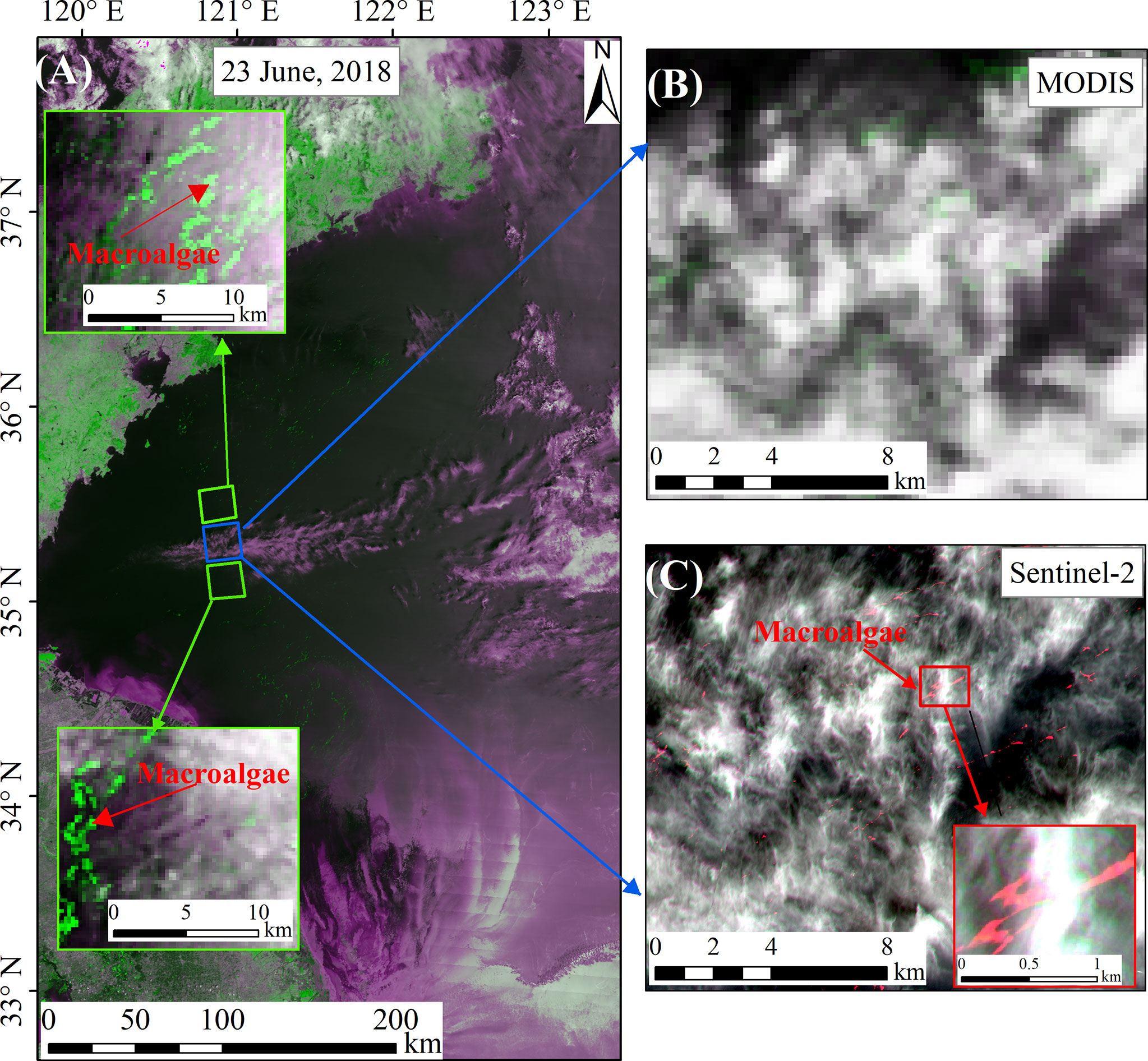
Figure 1 (A) Macroalgae shown in a false color composite by MODIS bands 1, 2, 1 acquired over the Yellow Sea on 23 June 2018. The green patches indicated by red arrows in green frame are floating green macroalgae, and the white patches in blue frame are clouds. (B) Details of blue frame shown in MODIS false color image. (C) Details of blue frame shown in Sentinel-2 false color image composite by bands 8, 4, 3 acquired on the same day as MODIS. In the false color images, the floating macroalgae patches are in red color.

To reduce the quantitative analysis error, we must obtain information about the macroalgae obscured by the cloud mask. How to do this is an interesting problem. Microwave remote sensing seems like an effective method because microwaves can penetrate clouds and fog due to their greater wavelength compared to visible and infrared radiation. As a result, the atmosphere has little effect on microwave remote sensing images. Nevertheless, the monitoring of MABs used by microwave remote sensing is still in its initial stage. The noise signal in microwave remote sensing data has an obvious impact on the interpretation of small macroalgae patches (Qiu and Lu, 2015), so currently it is mostly used as auxiliary monitoring data.

Another possible method is to reconstruct missing information obscured by clouds in remote sensing images and then detect macroalgae using the reconstructed image. Many methods for reconstructing missing information in remote sensing images have been previously proposed, including spatial-based methods (Ballester et al., 2001; Chan and Shen, 2001; Zhang et al., 2007; Shen et al., 2010; Yu et al., 2011), spectral-based methods (Rakwatin et al., 2008; Shen et al., 2010; Gladkova et al., 2012; Li et al., 2014a), and temporal-based methods (Julien and Sobrino, 2010; Zhu et al., 2011; Lorenzi et al., 2013; Li et al., 2014b; Zeng et al., 2014; Zhang et al., 2014b; Shen et al., 2015). Shen et al. (2015) summarized that the spatial-based methods are susceptible to blurring and usually fail to reconstruct large area of missing information, whereas the spectral-based methods usually target missing information problems caused by the sensor, such as black strip. Therefore, these two categories of methods are not suitable for the detection of macroalgae under cloud. The temporal-based methods are also not suitable obviously for the detection of macroalgae because macroalgae are constantly drifting (Cui et al., 2012; Harun-Al-Rashid and Yang, 2018).

For accurate MAB analysis and effective prevention and control, it is extremely important to reduce the impact of clouds on macroalgae estimates based on optical images. In this study, we propose a simple method to solve the impact of clouds on estimates of macroalgae area under clouds on MODIS imagery. It is based on the principle of the lowpass filter. Results detected by semi-simultaneous fine resolution images (GF-1, Sentienl-2 and Sentinel-1) in the same region are used for comparisons to determine the feasibility of the method.

2 Data and methods

2.1 Satellite data and processing

Fourteen satellite images (listed in Table 1) were used including eight Terra and Aqua MODIS images (250 m resolution), two GF-1 WFV images (16 m resolution), two Sentinel-2 MSI images (10 m resolution) and two Sentienl-1 SAR images. In this study, we used the Sentinel-1 Level-1 Interferometric Wide Swath (IW) Ground Range Detected (GRD) High Resolution product. The spatial resolution was 20 m × 22 m and the pixel spacing was 10 m × 10 m.

TABLE 1

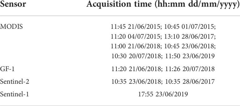
Table 1 Acquisition time of the satellite images.

Optical image preprocessing included georeferencing and atmospheric correction. The FLAASH (Fast Line of Sight Atmospheric Analysis of Spectral Hypercubes) atmospheric correction module via ENVI 5.3 software (Exelis Visual Information Solutions, Inc., Boulder, CO, USA) was applied to MODIS and GF-1 images to derive the reflectance (R, unitless), while the Sen2Cor atmospheric correction module from European Space Agency (ESA) was used on the Sentinel-2 images. For microwave images, the radiometric calibration module via SNAP (Sentinel Application Platform, ESA) was applied to Sentinel-1 images to derive the radar backscattering coefficient (NRCS, not converted to decibel value). The speckle filtering module and the range-doppler terrain correction via SNAP were also applied to Sentinel-1 images to reduce speckle impact and correct geometric distortion. All of the images were transformed into WGS_1984_UTM_Zone_51N coordinate system after preprocessing.

2.2 Macroalgae and cloud detection methods

2.2.1 Optical image macroalgae detection method

Many macroalgae information detection algorithms have been proposed by scholars based on the distinct spectral difference between natural seawater and macroalgae-covered seawater in the red light (Red) and near infrared (NIR) bands. The difference index algorithm, such as Difference Vegetation Index (DVI), Floating Algae Index (FAI), Virtual-Baseline Floating macroalgae Height (VB-FAH), is little affect by sunlight and aerosol changes and is not particularly sensitive to the accuracy of the atmospheric correction (Hu, 2009; Xing and Hu, 2016; Xing et al., 2018). In this work, the DVI index (Eq. (1)) is selected for detecting pixels containing macroalgae since MODIS 250m images only have two bands of Red and NIR.

$\begin{array}{ll}DVI=R_{NIR}-R_{Red}& (1)\end{array}$

where R_NIR is the reflectance at the near-infrared (NIR) band and R_Red is the red light band reflectance.

Given the significant variability in atmospheric turbidity, ocean background, and sun glint (Xing and Hu, 2016; Cui et al., 2018), a dynamic threshold of DVI was used to extract the macroalgae. The DVI images were segmented into small windows, and a set of thresholds was used to classify the macroalgae pixels window by window. For further details, please refer to Xing and Hu, 2016 and Xing et al., 2018.

Next, the macroalgae area (Area, km²) was derived by multiplying the pixel size of the satellite image (PS, km²) by the total number of pixels (N) that were identified as macroalgae (Cui et al., 2018), as shown in Eq. (2).

$\begin{array}{ll}\mathbf{Area}\mathbf{=}\mathbf{\text{N}}\times \mathbf{PS}& (2)\end{array}$

2.2.2 Microwave image macroalgae detection method

The Sentinel-1 IW-GRD image used in this study contained two polarization modes, VV and VH. From a qualitative perspective, the macroalgae pixels are shown more clearly with VV- (VV image) than VH-polarization (VH image) (Figure 2).

FIGURE 2

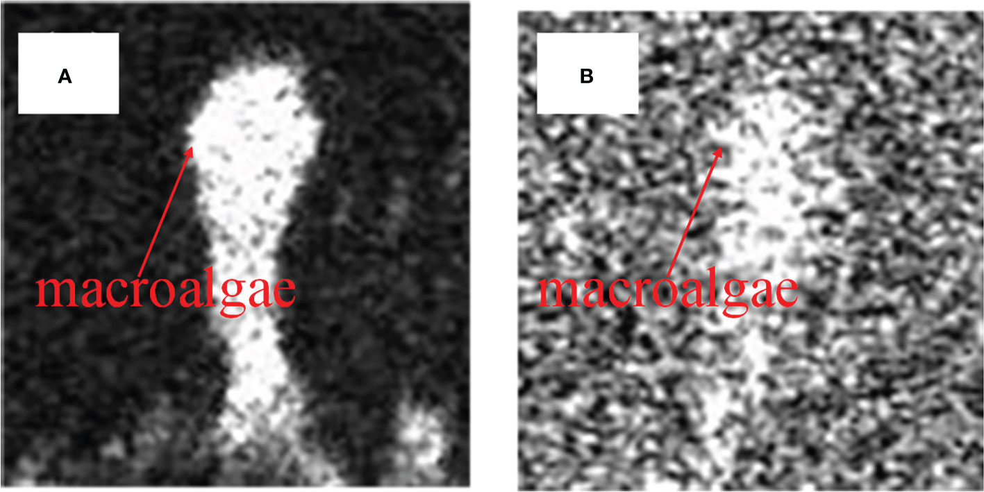
Figure 2 Comparison of visual interpretation quality of the floating macroalgae in two polarization modes of Sentinel-1: (A) VV; (B) VH.

From a quantitative perspective, the statistical analysis of NRCS including high NRCS pixels (i.e., pixels contained ships or islands), pixels containing macroalgae and pure seawater pixels showed that the mean value of high NRCS pixels is much larger than NRCS mean value of pixels containing macroalgae and pure seawater pixels (Figures 3A, B). Therefore, a high threshold was used to mask high NRCS pixels. The mean NRCS value of pixels containing macroalgae was larger than pure seawater pixels in both VV and VH images. The reason for this is that sea surface covered by macroalgae is rougher than a sea surface without macroalgae and the radar echo signal increases with increasing roughness. The difference between pixels containing macroalgae and pure seawater pixels was greater in the VV image than in the VH images (Figures 3A, B). The NRCS histogram analysis showed the same results (Figures 3C, D). Since it was easier to classify the floating macroalgae and other objects in the VV image than in the VH image. The VV image was used to detect the macroalgae. Given the variability in ocean background, a dynamic threshold of DVI was also used to extract the macroalgae. The detection details and the calculation method for macroalgae were same as for the optical image.

FIGURE 3

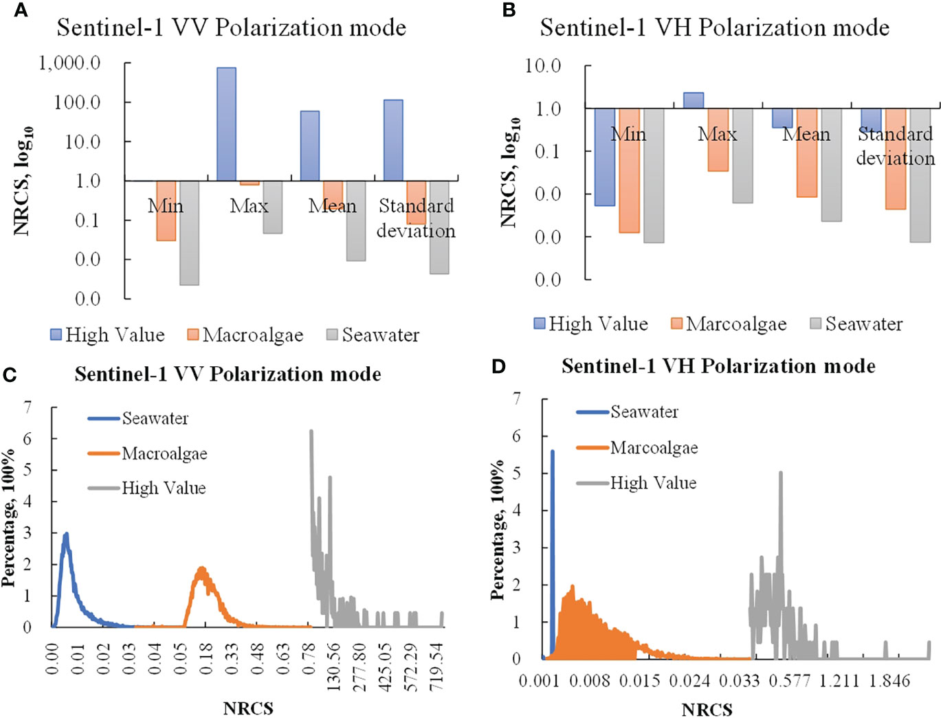
Figure 3 The radar backscattering coefficient (NRCS) comparison of pure seawater pixels (Seawater), pixels containing macroalgae (Macroalgae) and high NRCS pixels (High Value) in VV and VH polarization mode. (A, B) are the comparison of maximum value (Max), minimum value (Min), mean value (Mean) and standard deviation. (C, D) are the histogram comparison of Seawater, Macroalgae and High Value.

2.2.3 Consistency of macroalgae area detected from multi-sensor images

Macroalgae patches vary in size from centimetres to kilometres, which means that pixel-mixing is common for most remote sensing images (Xiao et al., 2017; Li et al., 2018). This situation can lead to biased results derived from images with different resolutions (Kim et al., 2018). Image pairs over the same macroalgae region with the same acquisition dates were selected to investigate the consistency in the retrieved macroalgae coverage area (Xing et al., 2019; An et al., 2021). The areas derived from different image pairs were then compared. Three linear regression functions (R² ≥ 0.9, MRD ≤ 25.71%) were performed on the areas derived from GF-1, Sentinel-2 and Sentinel-1 images and the areas from MODIS image (Figure 4). R² is the linear regression coefficient and MRD is the mean relative difference. MRD could be expressed by formulas as shown in Eq. (3).

$\begin{array}{ll} MRD=\frac{1}{N}{\sum }_{i=1}^N\frac{\left|(y_i-x_i)\right|}{x_i}\times 100\%& (3)\end{array}$

FIGURE 4

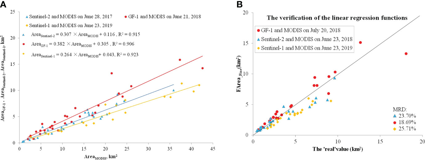
Figure 4 (A) Comparison in the macroalgae coverage areas derived from optical images of MODIS, GF-1, Sentinel-2 and Sentinel-1, i.e., Area_MODIS, Area_GF-1, Area_Sentinel-2, Area_Sentinel-1, respectively. (B) The verification of the linear regression functions in Figure (A). The ‘real’ values are the macroalgae area detected by fine resolution images (GF-1, Sentinel-2 and Sentinel-1), and FArea__Fine is the macroalgae fitted area converted by the macroalgae area detected by MODIS images based on the linear regression functions. MRD is the mean relative difference between FArea__Fine values and the ‘real’ values. The black line in figure is the 1:1 line.

where N is the number of image pairs. y is FArea_{_Fine}, i.e., the macroalgae fitted area converted by the macroalgae area detected by MODIS images based on the linear regression functions. x is the ‘real’ value, i.e., the macroalgae area detected by fine resolution images (GF-1, Sentinel-2 and Sentinel-1).

2.2.4 Cloud detection method

Clouds have significantly higher reflectance than underlying surfaces in the visible spectrum (Tan et al., 2000). Macroalgae has low reflectance in the red band because of the strong absorption caused by photosynthetic pigments (Dierssen et al., 2015). Thus, we also used a dynamic threshold method of the red band reflectance was used to detect clouds in MODIS images. The specific detection process was the same as for macroalgae. And the calculation method for clouds area (Area_{_cloud}) was also the same as for Area.

2.3 Simple method for estimating macroalgae area under clouds

We proposed a simple method for estimating macroalgae area under clouds (Area_{_cloud_GT}) based on the principle behind the lowpass filter. The lowpass filter is a filter commonly used for smoothing images in ENVI software. ENVI’s default low pass filter contains the same weights in each kernel element, replacing the center pixel value with an average of the surrounding values. The default kernel size was 3×3 (Deng, 2010). Figure 5 shows a simple estimation method of Area_{_cloud_GT} in the case of clouds surrounded by macroalgae. The process was as follows.

FIGURE 5

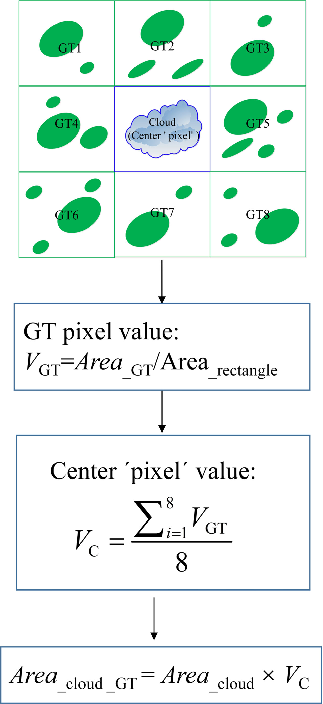
Figure 5 Methods for estimating macroalgae area under clouds (Area_{_cloud_GT}) in the case of clouds surrounded by macroalgae. These rectangles are the same size. In the surrounding rectangles (GT1-GT8), green ellipses represent different macroalgae patches. In the center rectangle (Cloud), the blue shape represents cloud patches.

First, we used a rectangle to determine the distribution range of the clouds. We designated this rectangle and eight identical rectangles containing macroalgae around the clouds as a central ‘pixel’ (Cloud) and eight adjacent ‘pixels’ (GT1~GT8).

Next, we calculated the macroalgae coverage rate of GT as the ratio of the macroalgae area to the corresponding rectangle area. We took this ratio as the ‘pixel’ value of GT. The average of the eight GT ‘pixels’ values from GT1 to GT8 was calculated and taken as the central ‘pixel’ value.

Finally, we derive the Area_{_cloud_GT} of this cloud by multiplying the cloud area (Area_{_cloud}) in the central ‘pixel’ region with the central ‘pixel’ value.

This method was used to calculate Area_{_cloud_GT} of eight MODIS images. The Area_{_cloud_GT} was converted into the macroalgae fitted area (FArea_{_cloud_GT}) of the corresponding fine resolution image. Next, FArea_{_cloud_GT} was compared with the macroalgae area estimated (Area_GF, Area_Sentinel-2, or Area_Sentinel-1) using semi-simultaneous fine resolution images in the same region. Area_GF (Area_Sentinel-2 or Area_Sentinel-1) was considered to be the ‘real’ value. The feasibility of the method was verified through the mean relative difference (MRD) between FArea_{_cloud_GT} and the ‘real’ value.

3 Results and discussion

3.1 Application of the simple method for estimating macroalgae area under clouds

In practice, it is not common for images to contain clouds surrounded by macroalgae. As a result, using the proposed method to estimate the Area_{_cloud_GT} will result in an underestimate. To avoid underestimating Area_{_cloud_GT}, we divided the distribution patterns of macroalgae and clouds into five cases. These five cases are as follows:

Case 1: If clouds are surrounded by macroalgae, the central ‘pixel’ value is the average of the eight GT ‘pixels’ values from GT1 to GT8, as shown in Figure 6B.

FIGURE 6

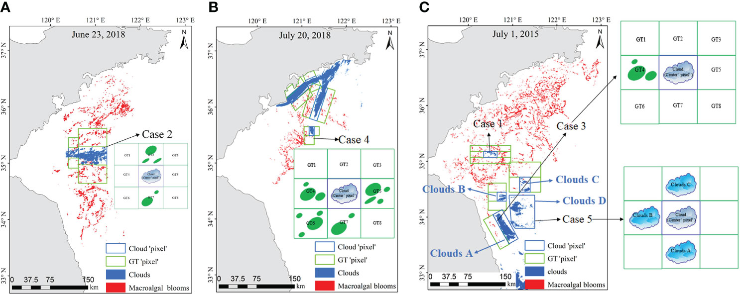
Figure 6 Application of the simple method for estimating macroalgae area under clouds under various scenarios. (A) The scenario of Case 2. (B) The scenario of Case 4. (C) The scenarios of Case 1, Case 3 and Case 5.

Case 2: If the rectangles in a south-north direction (or east-west or northeast-southwest, or northwest-southeast) of the clouds have macroalgae, the central ‘pixel’ value is the average of GT4 and GT5 (or GT2 and GT7, or GT3 and GT6, or GT1 and GT8), as shown in Figure 6A.

Case 3: If only one side of the cloud rectangle has macroalgae, the central ‘pixel’ value is the ‘pixel value’ of GT2 (north) [or GT7 (south) or GT4 (east) or GT5 (west)], as shown in Figure 6C.

Case 4: If the distribution of macroalgae around the clouds is scattered, the number of GT rectangles involved in the calculation can be judged on a case-by-case basis, as shown in Figure 6B. In this example, there are macroalgae in GT4, GT5, GT6, and GT7, so the average of these four ‘pixels’ is taken as the central ‘pixel’ value.

Case 5: If there is no macroalgae on one side of the clouds, while there is macroalgae on the other side of the clouds, there may be macroalgae under the clouds. As shown in Figure 6C, there is no macroalgae on the right side of cloud rectangle D, while there are macroalgae around adjacent cloud rectangles A, B, and C. The central ‘pixel’ value of cloud rectangles A, B, and C are first calculated according to the above four cases. The average of these three values is taken as the central ‘pixel’ value of cloud rectangle D.

Owing to the random distribution of clouds and macroalgae, there may be one of the above cases in a remote sensing image, such as June 23, 2018 (Figure 6A). There may also be two or three of the above cases, such as July 1, 2015 and July 20, 2018 (Figures 6B, C). There may also be four or all of the above cases, such as June 21, 2015 and July 4, 2015 (Figure 7).

FIGURE 7

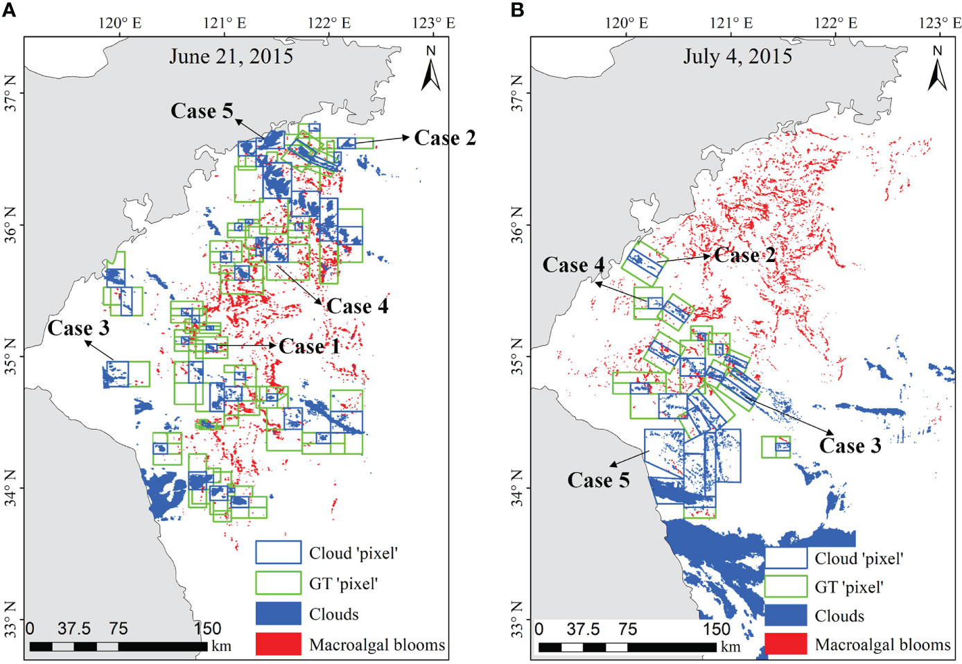
Figure 7 Application of the simple method for estimating macroalgae area under clouds under complex scenarios. (A) The scenario including four above cases; (B) The scenario including all above cases.

3.2 Verification of the simple method for estimating Area_{_cloud_GT}

The equations should be inserted in editable format from the equation editor. The Area_{_cloud_GT} derived from this simple method must be validated with field measurements to verify its accuracy. However, field verification is difficult because we cannot guarantee consistency between the region covered by aerial survey (or ship survey) and the area of clouds on an image. Instead, we selected fifteen pairs of cloud sub-regions on MODIS images and fine spatial images acquired on the same day to verify the feasibility of the simple method of estimating Area_{_cloud_GT}, as shown in Figure 8A.

FIGURE 8

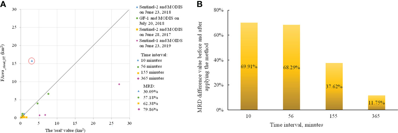
Figure 8 (A) The verification results of the simple method for estimating macroalgae area under clouds on MODIS imagery. The ‘real’ values are the macroalgae area detected by fine resolution images. FArea_{_cloud_GT} is the macroalgae fitted area converted by Area_cloud_GT, and Area_{_cloud_GT} is the macroalgae area under clouds estimated by the method. The black line in figure is the 1:1 line. (B) The MRD difference value before and after applying the method.

The FArea_{_cloud_GT} on MODIS images was obtained according to section 2.3 and 3.1, and compared with the ‘real’ value, i.e., Area_GF (Area_Sentinel-2 or Area_Sentinel-1). As shown in Figure 8A, when the time interval was within 10 minutes, FArea_{_cloud_GT} converted from MODIS images was relatively close to the ‘real’ value except for the individual regions in red circle. The MRD between FArea_{_cloud_GT} and the ‘real’ value was 30.09%. When the time interval was within about one hour, the MRD increased significantly to 57.18%. When the time interval was over three hours, the MRD was more than 60%. The increase in MRD with time is easily understood. The macroalgae is constantly moving (Cui et al., 2012; Harun-Al-Rashid and Yang, 2018) and macroalgal aggregation morphology is changing at any time. In addition, we used here only extract the surface floating macroalgae, and less considering of the distribution of macroalgae in the upper water column because of the limitations of the remote sensing image, so the longer the time interval, the larger the MRD. From this study, we can conclude that the simple method has a relatively good accuracy.

For individual regions in red circle, the difference between FArea_{_cloud_GT} and the ‘real’ value is extremely obvious. We speculate that there are two possible reasons besides time interval. One reason is the difference in macroalgal aggregation morphology caused by sea surface wind and sea surface current (Xu et al., 2016; Cao et al., 2019). This difference can affect the calculation result of the macroalgae coverage rate, causing the larger MRD between FArea_{_cloud_GT} and the ‘real’ value. The other reason is the impact of cloud top height, cloud optical thickness, cloud effective particle radius, and other factors. These factors can affect the reflectance of underlying surfaces (Tan et al., 2000), and thus affect macroalgae detection, leading to uncertainty in FArea_{_cloud_GT}.

The range of MRD was 10.89% to 87.26% after applying the simple method for estimating macroalgae area under clouds on MODIS imagery, while the range of MRD was 74.83% to 100% before applying the method. The estimation accuracy of semi-simultaneous cloud sub-regions was improved by 11.75% to 69.91% on average (Figure 8B). These results indicate the method can significantly improve the estimation accuracy of macroalgae area under cloudy conditions and has an evident effect in reducing the impact of clouds on the macroalgae area estimated on MODIS imagery.

4 Conclusions and prospective

Optical remote sensing images are seriously affected by clouds. Most current research about macroalgae area and biomass does not consider whether the sea surface under clouds is covered by macroalgae. This omission causes an increase in the difference between the estimated and actual biomass. The novelty of this study is that a simple method for estimating macroalgae area under clouds on MODIS imagery is proposed to address this challenge. The accuracy of the method is verified by a comparison of the estimation results and results detected by semi-simultaneous fine resolution images in the same region. The verification results show that the simple method has a relatively good accuracy, and can provide a technological reference for MAB quantitative analysis.

This method can be extended to other remote sensing images with coarse spatial resolution, such as GOCI. In practical application, the MRD between the ‘real’ results and the estimation results using this method may be larger in individual regions because of the impacts from macroalgal aggregation morphology, cloud optical thickness, cloud effective particle radius, and other factors. Further study is needed to reduce the impact of these factors to improve the method.

Data availability statement

The original contributions presented in the study are included in the article/supplementary material. Further inquiries can be directed to the corresponding author.

Author contributions

Conceptualization, DA and QX; methodology, DA; formal analysis, QX, DA, and DY; writing—original draft preparation, DA and QX; writing—review and editing, DY, QX, and SP. All authors have read and agreed to the published version of the manuscript.

Funding

This research was funded by, the Chinese Academy of Science Strategic Priority Research Program—the Big Earth Data Science Engineering Project (No. XDA19060203 and XDA19060501), the National Natural Science Foundation of China (No.42076188, 41676171, 42106172 and 41911530), the National Key Research and Development Program of China (No. 2017YFC1404802), Natural Science Foundation of Shandong Province (No. ZR2021QD135, ZR2019PD021), the Key Research and Development Program of Shandong (No. 2019GHY112017), State Key Laboratory of Tropical Oceanography, South China Institute of Oceanology, Chinese Academy of Sciences (No. LTO2017), the Project plan of pilot project of integration of science, education and Industry (No.2022GH004, 2022PY041), the Foundation of Institute of Oceanographic Instrumentation, Shandong Academy of Sciences (No. HYPY202107), and the University-Industry Collaborative Education Program (No. 202102245036 and 202101044002).

Acknowledgments

Thanks to China Center for Resources Satellite Data and Application and NASA’s Goddard Space Flight Center for providing GF-1 and MODIS data, and to European Space Agency for Sentinel-2 and Sentinel-1 data. The authors are grateful for the encouragement and suggestions from reviewers.

Conflict of interest

The authors declare that the research was conducted in the absence of any commercial or financial relationships that could be construed as a potential conflict of interest.

Publisher’s note

All claims expressed in this article are solely those of the authors and do not necessarily represent those of their affiliated organizations, or those of the publisher, the editors and the reviewers. Any product that may be evaluated in this article, or claim that may be made by its manufacturer, is not guaranteed or endorsed by the publisher.

References

An D., Yu D., Zheng X., Zhou Y., Meng L., Xing Q. (2021). Monitoring the dissipation of the floating green macroalgae blooms in the yellow Sea, (2007–2020) on the basis of satellite remote sensing. Remote Sensing. 13 (19), 3811. doi: 10.3390/rs1319381

CrossRef Full Text | Google Scholar

Ballester C., Bertalmio M., Caselles V., Sapiro G., Verdera J. (2001). Filling-in by joint interpolation of vector fields and gray levels. IEEE Trans. Image. Processing. 10 (8), 1200–1211. doi: 10.1109/83.935036

CrossRef Full Text | Google Scholar

Cao Y., Wu Y., Fang Z., Cui X., Liang J., Song X. (2019). Spatiotemporal patterns and morphological characteristics of Ulva prolifera distribution in the yellow Sea, China in 2016–2018. Remote Sensing. 11 (4), 445. doi: 10.3390/rs11040445

CrossRef Full Text | Google Scholar

Chan T., Shen J. (2001). Nontexture inpainting by curvature-driven diffusions. J. Visual Commun. Image. Representation. 12 (4), 436–449. doi: 10.1006/jvci.2001.0487

CrossRef Full Text | Google Scholar

Chen Y., Sun D., Zhang H., Wang S., Qiu Z., He Y. (2020). Remote-sensing monitoring of green tide and its drifting trajectories in yellow Sea based on observation data of geostationary ocean color imager. Acta Optica. Sin. 40 (03), 7–19. doi: 10.3788/AOS202040.0301001

CrossRef Full Text | Google Scholar

Cui T., Liang X., Gong J., Tong C., Xiao Y., Liu R., et al. (2018). Assessing and refining the satellite-derived massive green macro-algal coverage in the yellow Sea with high resolution images. ISPRS. J. Photogramm. Remote Sensing. 144, 315–324. doi: 10.1016/j.isprsjprs.2018.08.001

CrossRef Full Text | Google Scholar

Cui B., Zhang H., Jing W., Liu H., Cui J. (2022). SRSe-net: Super-resolution-based semantic segmentation network for green tide extraction. Remote Sensing. 14 (3), 710. doi: 10.3390/rs14030710

CrossRef Full Text | Google Scholar

Cui T., Zhang J., Sun L., Jia Y., Zhao W., Wang Z., et al. (2012). Satellite monitoring of massive green macroalgae bloom (GMB): Imaging ability comparison of multi-source data and drifting velocity estimation. Int. J. Remote Sensing. 33 (17), 5513–5527. doi: 10.1080/01431161.2012.663112

CrossRef Full Text | Google Scholar

Deng S. (2010). ““Image enhancement”,” in ENVI remote sensing image processing methods (Beijing: Science Press), 103.

Google Scholar

Dierssen H., Chlus A., Russell B. (2015). Hyperspectral discrimination of floating mats of seagrass wrack and the macroalgae sargassum in coastal waters of greater Florida bay using airborne remote sensing. Remote Sens. Environment. 167, 247–258. doi: 10.1016/j.rse.2015.01.027

CrossRef Full Text | Google Scholar

Feng S., Li F., Li S. (1998). “Regional oceanography of china's coastal waters”,” in Introduction to marine science (Beijing: Higher Education Press), 329.

Google Scholar

Gladkova I., Grossberg M., Shahriar F., Bonev G., Romanov P. (2012). Quantitative restoration for MODIS band 6 on aqua. IEEE Trans. Geosci. Remote Sensing. 50 (6), 2409–2416. doi: 10.1109/TGRS.2011.2173499

CrossRef Full Text | Google Scholar

Harun-Al-Rashid A., Yang C. (2018). Hourly variation of green tide in the yellow Sea during summer 2015 and 2016 using geostationary ocean color imager data. Int. J. Remote Sensing. 39 (13), 4402–4415. doi: 10.1080/01431161.2018.1457228

CrossRef Full Text | Google Scholar

Hu C. (2009). A novel ocean color index to detect floating algae in the global oceans. Remote Sens. Environment. 113 (10), 2118–2129. doi: 10.1016/j.rse.2009.05.012

CrossRef Full Text | Google Scholar

Hu C., He M. (2008). Origin and offshore extent of floating algae in Olympic sailing area. Eos. Trans. Am. Geophys. Union. 89 (33), 302–303. doi: 10.1029/2008EO330002

CrossRef Full Text | Google Scholar

Hu L., Hu C., He M. (2017). Remote estimation of biomass of Ulva prolifera macroalgae in the yellow Sea. Remote Sens. Environment. 192, 217–227. doi: 10.1016/j.rse.2017.01.037

CrossRef Full Text | Google Scholar

Hu C., Li D., Chen C., Ge J., Muller-Karger F., Liu J., et al. (2010). On the recurrent Ulva prolifera blooms in the yellow Sea and East China Sea. J. Geophys. Res.: Oceans. 115, C05017. doi: 10.1029/2009JC005561

CrossRef Full Text | Google Scholar

Hu L., Zeng K., Hu C., He M. (2019). On the remote estimation of Ulva prolifera areal coverage and biomass. Remote Sens. Environment. 223, 194–207. doi: 10.1016/j.rse.2019.01.014

CrossRef Full Text | Google Scholar

Julien Y., Sobrino J. (2010). Comparison of cloud-reconstruction methods for time series of composite NDVI data. Remote Sens. Environment. 114 (3), 618–625. doi: 10.1016/j.rse.2009.11.001

CrossRef Full Text | Google Scholar

Kim K., Shin J., Ryu J. (2018). Application of multi-satellite sensors to estimate the green-tide area. Korean. J. Remote Sens. 34 (2\_2), 339–349. doi: 10.7780/kjrs.2018.34.2.2.4

CrossRef Full Text | Google Scholar

Li X., Shen H., Zhang L., Zhang H., Yuan Q. (2014a). Dead pixel completion of aqua MODIS band 6 using a robust m-estimator multiregression. IEEE Geosci. Remote Sens. Lett. 11 (4), 768–772. doi: 10.1109/LGRS.2013.2278626

CrossRef Full Text | Google Scholar

Li X., Shen H., Zhang L., Zhang H., Yuan Q., Yang G. (2014b). Recovering quantitative remote sensing products contaminated by thick clouds and shadows using multitemporal dictionary learning. IEEE Trans. Geosci. Remote Sensing. 52 (11), 7086–7098. doi: 10.1109/TGRS.2014.2307354

CrossRef Full Text | Google Scholar

Liu D., Keesing J. K., Xing Q., Shi P. (2009). World’s largest macroalgal bloom caused by expansion of seaweed aquaculture in China. Mar. pollut. Bull. 58 (6), 888–895. doi: 10.1016/j.marpolbul.2009.01.013

PubMed Abstract | CrossRef Full Text | Google Scholar

Li L., Zheng X., Wei Z., Zou J., Xing Q. (2018). A spectral-mixing model for estimating sub-pixel coverage of sea-surface floating macroalgae. Atmosphere-Ocean 56 (4), 296–302. doi: 10.1080/07055900.2018.1509834

CrossRef Full Text | Google Scholar

Lorenzi L., Melgani F., Mercier G. (2013). Missing-area reconstruction in multispectral images under a compressive sensing perspective. IEEE Trans. Geosci. Remote Sensing. 51 (7), 3998–4008. doi: 10.1109/TGRS.2012.2227329

CrossRef Full Text | Google Scholar

Min S., Oh H., Hwang J., Suh Y., Park M., Shin J., et al. (2017). Tracking the movement and distribution of green tides on the yellow Sea in 2015 based on GOCI and landsat images. Korean. J. Remote Sensing. 33 (1), 97–109. doi: 10.1109/TGRS.2012.2227329

CrossRef Full Text | Google Scholar

Morand P., Merceron M. (2005). Macroalgal population and sustainability. J. Coast. Res. 21 (5), 1009–1020. doi: 10.2112/04-700A.1

CrossRef Full Text | Google Scholar

Qi L., Hu C., Xing Q., Shang S. (2016). Long-term trend of Ulva prolifera blooms in the western yellow Sea. Harmful. Algae. 58, 35–44. doi: 10.1016/j.hal.2016.07.004

PubMed Abstract | CrossRef Full Text | Google Scholar

Qiu Z., Li Z., Bilal M., Wang S., Sun D., Chen Y. (2018). Automatic method to monitor floating macroalgae blooms based on multilayer perceptron: Case study of yellow Sea using GOCI images. Optics. Express. 26 (21), 26810–26829. doi: 10.1364/OE.26.026810

PubMed Abstract | CrossRef Full Text | Google Scholar

Qiu Y., Lu J. (2015). Advances in the monitoring of Enteromorpha prolifera using remote sensing. Acta Ecol. Sin. 35 (15), 4977–4985. doi: 10.5846/stxb201309232339

CrossRef Full Text | Google Scholar

Rakwatin P., Takeuchi W., Yasuoka Y. (2008). Restoration of aqua MODIS band 6 using histogram matching and local least squares fitting. IEEE Trans. Geosci. Remote Sensing. 47 (2), 613–627. doi: 10.1109/TGRS.2008.2003436

CrossRef Full Text | Google Scholar

Shen H., Liu Y., Ai T., Wang Y., Wu B. (2010). Universal reconstruction method for radiometric quality improvement of remote sensing images. International Journal of Applied Earth Observation and Geoinformation 12 (4), 278–286. doi: 10.1016/j.jag.2010.04.002

CrossRef Full Text | Google Scholar

Shen H., Zeng C., Zhang L. (2010). Recovering reflectance of aqua MODIS band 6 based on within-class local fitting. IEEE J. Selected. Topics. Appl. Earth Observ. Remote Sensing. 4 (1), 185–192. doi: 10.1109/JSTARS.2010.2077620

CrossRef Full Text | Google Scholar

Shen H., Li X., Cheng Q., Zeng C., Yang G., Li H., et al (2015). Missing information reconstruction of remote sensing data: A technical review. IEEE Geoscience and Remote Sensing Magazine 3 (3), 61–85. doi: 10.1109/MGRS.2015.2441912

CrossRef Full Text | Google Scholar

Smetacek V., Zingone A. (2013). Green and golden seaweed tides on the rise. Nature 504 (7478), 84–88. doi: 10.1038/nature12860

PubMed Abstract | CrossRef Full Text | Google Scholar

Song X., Huang R., Yuan K., Zhao Y., Wen R., Zhang H. (2015). Characteristics of the green tide disaster of east Shandong peninsula. Mar. Environ. Sci. 34 (3), 391–395. doi: 10.13634/j.cnki.mes.2015.03.012

CrossRef Full Text | Google Scholar

Son Y., Min J., Ryu J. (2012). Detecting massive green algae (Ulva prolifera) blooms in the yellow Sea and East China Sea using geostationary ocean color imager (GOCI) data. Ocean. Sci. J. 47 (3), 359–375. doi: 10.1007/s12601-012-0034-2

CrossRef Full Text | Google Scholar

Sun S., Wang F., Li C., Qin S., Zhou M., Ding L., et al. (2008). Emerging challenges: Massive green algae blooms in the yellow Sea. Nat. Precedings. 3, 1–13. doi: 10.1038/npre.2008.2266.1

CrossRef Full Text | Google Scholar

Tan J., Zhou H., Yang C. (2000). Research and establishment in operation system of cloud detection and rehabilitation applied to NOAA satellite. Remote Sens. Technol. Application. 15 (4), 228–231. doi: 10.11873/j.issn.1004-0323.2000.4.228

CrossRef Full Text | Google Scholar

Wang M., Hu C., Barnes B., Mitchum G., Lapointe B., Montoya J. (2019). The great Atlantic sargassum belt. Science 365 (6448), 83–87. doi: 10.1126/science.aaw7912

PubMed Abstract | CrossRef Full Text | Google Scholar

Xiao Y., Zhang J., Cui T. (2017). High-precision extraction of nearshore green tides using satellite remote sensing data of the yellow Sea, China. Int. J. Remote Sensing. 38 (6), 1626–1641. doi: 10.1080/01431161.2017.1286056

CrossRef Full Text | Google Scholar

Xiao Y., Zhang J., Cui T., Gong J., Liu R., Chen X., et al. (2019). Remote sensing estimation of the biomass of floating Ulva prolifera and analysis of the main factors driving the interannual variability of the biomass in the yellow Sea. Mar. pollut. Bull. 140, 330–340. doi: 10.1016/j.marpolbul.2019.01.037

PubMed Abstract | CrossRef Full Text | Google Scholar

Xing Q., An D., Zheng X., Wei Z., Wang X., Li L., et al. (2019). Monitoring seaweed aquaculture in the yellow Sea with multiple sensors for managing the disaster of macroalgal blooms. Remote Sens. Environment. 231, 111279. doi: 10.1016/j.rse.2019.111279

CrossRef Full Text | Google Scholar

Xing Q., Hu C. (2016). Mapping macroalgal blooms in the yellow Sea and East China Sea using HJ-1 and landsat data: Application of a virtual baseline reflectance height technique. Remote Sens. Environment. 178, 113–126. doi: 10.1016/j.rse.2016.02.065

CrossRef Full Text | Google Scholar

Xing Q., Hu C., Tang D., Tian L., Tang S., Wang X., et al. (2015). World’s largest macroalgal blooms altered phytoplankton biomass in summer in the yellow Sea: Satellite observations. Remote Sensing. 7 (9), 12297–12313. doi: 10.3390/rs70912297

CrossRef Full Text | Google Scholar

Xing Q., Wu L., Tian L., Cui T., Li L., Kong F., et al. (2018). Remote sensing of early-stage green tide in the yellow Sea for floating-macroalgae collecting campaign. Mar. pollut. Bull. 133, 150–156. doi: 10.1016/j.marpolbul.2018.05.035

PubMed Abstract | CrossRef Full Text | Google Scholar

Xing Q., Zheng X., Shi P., Hao J., Yu D., Liang S., et al. (2011). Monitoring “Green tide”in the yellow Sea and the East China Sea using multi-temporal and multi-source remote sensing images. Spectrosc. Spectral. Analysis. 31 (6), 1644–1647. doi: 10.3964/j.issn.1000-0593(2011)06-1644-04

CrossRef Full Text | Google Scholar

Xu Q., Zhang H., Cheng Y., Zhang S., Zhang W. (2016). Monitoring and tracking the green tide in the yellow Sea with satellite imagery and trajectory model. IEEE J. Selected. Topics. Appl. Earth Observ. Remote Sensing. 9 (11), 5172–5181. doi: 10.1109/JSTARS.2016.2580000

CrossRef Full Text | Google Scholar

Xu Q., Zhang H., Ju L., Chen M. (2014). Interannual variability of Ulva prolifera blooms in the yellow Sea. Int. J. Remote Sensing. 35 (11-12), 4099–4113. doi: 10.1080/01431161.2014.916052

CrossRef Full Text | Google Scholar

Ye N., Zhang X., Mao Y., Liang C., Xu D., Zou J., et al. (2011). ‘Green tides’ are overwhelming the coastline of our blue planet: taking the world’s largest example. Ecol. Res. 26 (3), 477–485. doi: 10.1007/s11284-011-0821-8

CrossRef Full Text | Google Scholar

Ye N., Zhuang Z., Jin X., Wang Q., Zhang X., Li D., et al. (2008). China Is on the tracking enteromorpha spp. forming green tide. Nat. Precedings 3, 1–10. doi: 10.1038/npre.2008.2352.1

CrossRef Full Text | Google Scholar

Yu C., Chen L., Su L., Fan M., Li S. (2011). “Kriging interpolation method and its application in retrieval of MODIS aerosol optical depth,” in 2011 19th International Conference on Geoinformatics. (IEEE) 1–6. doi: 10.1109/GeoInformatics.2011.5981052

CrossRef Full Text | Google Scholar

Zeng C., Shen H., Zhong M., Zhang L., Wu P. (2014). Reconstructing MODIS LST based on multitemporal classification and robust regression. IEEE Geosci. Remote Sens. Lett. 12 (3), 512–516. doi: 10.1109/LGRS.2014.2348651

CrossRef Full Text | Google Scholar

Zhang J., Clayton M., Townsend P. (2014). Missing data and regression models for spatial images. IEEE Trans. Ggeosci. Remote Sensing. 53 (3), 1574–1582. doi: 10.1109/TGRS.2014.2345513

CrossRef Full Text | Google Scholar

Zhang C., Li W., Travis D. (2007). Gaps-fill of SLC-off landsat ETM+ satellite image using a geostatistical approach. Int. J. Remote Sensing. 28 (22), 5103–5122. doi: 10.1080/01431160701250416

CrossRef Full Text | Google Scholar

Zhang H., Sun D., Li J., Qiu Z., Wang S., He Y. (2016). Remote sensing algorithm for detecting green tide in China coastal waters based on GF1-WFV and HJ-CCD data. Acta Optica. Sin. 36 (6), 601004. doi: 10.3788/AOS201636.0601004

CrossRef Full Text | Google Scholar

Zhou M., Liu D., Anderson D., Valiela I. (2015). Introduction to the special issue on green tides in the yellow Sea. Estuarine. Coast. Shelf. Sci. 163, 3–8. doi: 10.1016/j.ecss.2015.06.023

CrossRef Full Text | Google Scholar

Zhou Y., Zhou B., Gai Y. (2014). Ulva prolifera monitoring study in the yellow Sea from multi-temporal remote sensing images. Appl. Mechanics. Materials. 675–677, 1201–1206. doi: 10.4028/www.scientific.net/AMM.675-677.1201

CrossRef Full Text | Google Scholar

Zhu W., Pan Y., He H., Wang L., Mou M., Liu J. (2011). A changing-weight filter method for reconstructing a high-quality NDVI time series to preserve the integrity of vegetation phenology. IEEE Trans. Geosci. Remote Sensing. 50 (4), 1085–1094. doi: 10.1109/TGRS.2011.2166965

CrossRef Full Text | Google Scholar