Effects of the Kuroshio on internal tides in the Luzon Strait: A model study

Internal tides have a great impact on the meridional overturning circulation and climate variability through contributing to diapycnal mixing. The Luzon Strait (LS) is one of the most important sites of internal tide generation in the global ocean. In this study, we evaluate the effect of the Kuroshio on the M2 and K1 internal tides in both summer and winter seasons in the South China Sea (SCS), particularly within the LS. High-resolution ocean numerical simulations with the Kuroshio Current were compared with those without. We found that the Kuroshio has negligible impact on the generation site of internal tides. Compared to seasonal variability in the total barotropic to baroclinic conversion rate over the LS, the Kuroshio has relatively little influence. However, the Kuroshio flow strongly guides the propagating direction of the internal tides from the LS into the SCS. The Kuroshio also substantially decreases the southward energy fluxes going out of the LS. For both M2 and K1 tides, turning off the Kuroshio leads to a weaker energy exchange between the background shear and internal tides. Turning off the Kuroshio also weakens the divergence of internal tide energy due to the advection of background flow. Thus, our results reveal a non-negligible effect of the Kuroshio on the internal tides in the LS. If one aims to realistically simulate, or better understand, internal tides, these results indicate that one should include realistic oceanic circulation fields.

1 Introduction

Oceanic circulation can be greatly affected by internal tides, which often arise when barotropic tidal currents pass over topography in stratified oceans (Wang et al., 1991; Lamb, 1994; Munk and Wunsch, 1998; Simmons et al., 2004; Vlasenko et al., 2005). Although low-mode internal tides can propagate over thousands of kilometers, high-mode internal tides often break up and dissipate (Klymak et al., 2012). This break up of internal tides leads to strong turbulence and diapycnal mixing, and thus influences the abyssal stratification and global meridional overturning circulation (Munk and Wunsch, 1998; Egbert and Ray, 2000; St. Laurent, 2008). For example, Simmons et al. (2004) showed that internal tides contribute up to ~1 TW of energy to sustain global abyssal mixing.

The Luzon Strait (LS), connecting the South China Sea (SCS) to the Western Pacific, consists of double meridional submarine ridges (Hengchun and Lanyu ridges). Hereafter, for analyses, we will define the LS region as 120°E-123°E, 18°N-22°N. Strong internal tides with vertical isopycnal displacements of up to 150 m have been observed in this region (Duda et al., 2004; Ramp et al., 2004). In fact, the strong stratification and barotropic tidal action make the LS one of the world ocean’s most important energy sources of internal tides and internal solitary waves (Guo and Chen, 2014; Alford et al., 2015). The large internal tide energy is also partly due to the double-ridge resonance mechanism (Zu et al., 2008; Alford et al., 2011; Buijsman et al., 2014). These locally generated internal tides can radiate both westward into the SCS and eastward into the Pacific Ocean. The observed time-averaged westward energy flux can reach 40 ± 8 kW m^-1, larger than other known estimates in the world (Alford et al., 2015). The low-mode internal tides can propagate more than 1000 km to the interior of the SCS and the Pacific Ocean (Zhao, 2014; Xu et al., 2016; Liu et al., 2017). During their propagation, these internal tides interact with other internal tides, such as those from the Mariana Island Arc and Ryukyu Ridge (Niwa and Hibiya, 2004; Kerry et al., 2013; Xu et al., 2016; Wang et al., 2018).

Internal tides in the LS region can be affected by the warm, salty Kuroshio. The Kuroshio is a western boundary current in the North Pacific, starting from the North Equatorial Current and flowing northward along the east coast of the Philippines. When the Kuroshio passes the SCS, part of the flow invades the SCS through the LS. Satellite observations reveal that, at any given time, the way that the Kuroshio invades can be one of three dominant types: the leaping path, the leaking path, or the looping path (Figure 1). The invasion path can change from one type to another within a few weeks (Nan et al., 2011). The strength of the Kuroshio invasion varies seasonally, being stronger in winter than in summer (Wyrtki, 1961; Shaw, 1991; Centurioni et al., 2004; Nan et al., 2015). The Kuroshio intrusion, which drives strong background subtidal currents, shifts the tilted thermocline to the west, thus changing the background stratification and affecting the generation, variability, and energy balance of internal tides in the LS (Varlamov et al., 2015; Li et al., 2016; Song and Chen, 2020). Using observations and numerical simulations, Ma et al. (2013) showed that the Kuroshio can influence the westward energy flux of internal tides in the LS by modifying the stratification and isopycnal slope. Besides internal tides in the LS, the Kuroshio also has significant impact on internal tides in other regions, such as northeast of Taiwan and the Izu-Ogasawara Ridge off the coast of Japan (Masunaga et al., 2018; Chang et al., 2019; Masunaga et al., 2019).

FIGURE 1

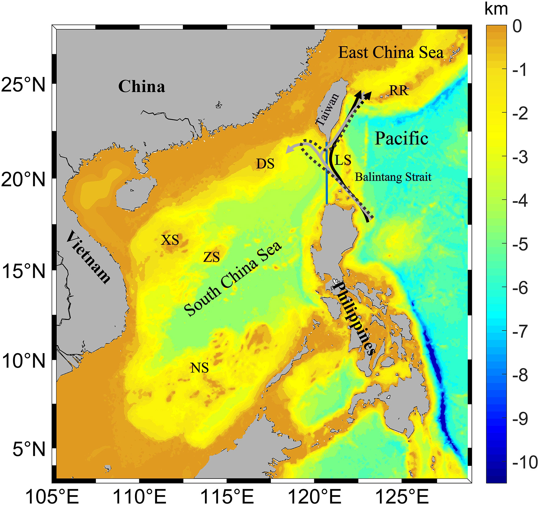
Figure 1 Bathymetry of the modelling domain. LS: Luzon Strait, DS: Dongsha Islands, XS: Xisha Islands, ZS: Zhongsha Islands, NS: Nansha Islands, RR: Ryukyu ridge. Arrows depict the type of Kuroshio invasion into the SCS (adapted from Nan et al., 2011): leaping path (solid black arrow), leaking path (solid gray arrow), and looping path (dashed black arrow). The blue line indicates the meridional section at 120.75°E, 18.5°N - 22°N, which is discussed in section 3.1.

Several numerical studies have examined the effects of the Kuroshio on internal tides in the LS (Jan et al., 2012; Varlamov et al., 2015; Song and Chen, 2020). A study using idealized topography found that both the location and magnitude of the Kuroshio can influence the generation and propagation of M₂ and K₁ internal tides (Jan et al., 2012). However, it is unclear whether their conclusions hold up for cases with realistic topography. Later, Varlamov et al. (2015) found that the M₂ tide variability in the LS can be modulated by the Kuroshio intrusion into the SCS. However, they used eight constituents of tidal forcing to force the model at the open boundary. Similarly, Song and Chen (2020) used simulations with all tidal constituents to examine the role of nonuniform stratification in modulating internal tides in the Northwest Pacific. However, M₂ and K₁ internal tides can respond to the Kuroshio in different ways. For example, Jan et al. (2012) found that the westward baroclinic energy flux of K₁ tides responds to the Kuroshio in an opposite way to that of M₂ tides. Therefore, it is important to consider each tidal constituent separately and evaluate whether the internal tide response to the Kuroshio is sensitive to the tidal constituents used for forcing. In addition, Song and Chen (2020) argued that nonlinearity in the baroclinic tide energy budget is important. Yet, the role of nonlinearity in the response of internal tides to the Kuroshio needs to be clarified and documented.

Inspired by these previous findings, we evaluate here the effects of the Kuroshio on the generation and propagation of internal tides in the SCS, particularly in the LS region. Specifically, we use the coastal and regional ocean community model (CROCO) to simulate the semidiurnal (M₂) or the diurnal (K₁) tidal forcing in summer and winter. The case with the Kuroshiois compared with the case without the Kuroshio for evaluating the energy conversion rate, the internal tide energy flux, as well as the baroclinic tide energy budget. We show that the Kuroshio greatly modulates the propagation direction of internal tides. The energy budget of internal tides is also sensitive to the existence of the Kuroshio.

This paper is organized as follows. Section 2 introduces the model configuration, data processing methods, and the energy diagnostic framework. Section 3 validates the model. Section 4 presents results about the effects of the Kuroshio on internal tides. Section 5 gives the summary and conclusion.

2 Method and diagnostic framework

2.1 Ocean model description

We use the CROCO model (version 1.0, https://www.croco-ocean.org), which has proved useful for simulating internal tides (Guo et al., 2020a; Guo et al., 2020b). It is a split-explicit, free-surface ocean model based on the Boussinesq approximation. In our application, the wavelength of internal tides is much larger than the water depth (Vitousek and Fringer, 2011), and so following previous studies, we use the hydrostatic configuration (Jan et al., 2007; Jan et al., 2008; Rainville et al., 2010; Osborne et al., 2011; Powell et al., 2012; Kerry et al., 2013; Liu et al., 2019).

Our model has 40 vertical non-uniform sigma layers and a horizontal resolution of 1/30°. In our simulation domain (Figure 1), topography is complex, with multiple islands, ridges, continental slopes and deep-sea basins. The topography data is from GEBCO2019 (general bathymetric chart of the oceans, https://www.gebco.net/), then further smoothed to avoid the pressure-gradient errors arising from sigma coordinates (Niwa and Hibiya, 2004). The minimum and maximum depths are 20 and 6000 m. To represent vertical mixing, we use the K-profile parameterization (KPP) mixing scheme (Large et al., 1994). For horizontal mixing, we use the Laplacian method. The explicit lateral viscosity is set to be 10 m² s^-1 and the bilaplacian background diffusivity is 20 m² s^-1 in the implicit diffusion of advection scheme (Cambon et al., 2018).

Table 1 summarizes the setup of numerical experiments. All of the experiments exclude both wind forcing and heat flux. The model initial and boundary conditions for temperature, salinity, velocity and sea level, for all of the experiments are from the HYCOM 10-year (2002-2011) monthly-averaged reanalysis dataset at a horizontal resolution of 1/12° (GOFS 3.0, https://www.hycom.org/dataserver/gofs-3pt0/reanalysis). For the winter cases in Table 1, the 10-year monthly-averaged HYCOM outputs in January are used as the initial and boundary conditions; whereas for the summer cases, the July HYCOM outputs are used. In the control run (CtrlS and CtrlW in Table 1), tidal forcing is not specified at the open boundaries and thus the internal tides do not exist. For other experiments (cases with or without the Kuroshio in Table 1), they are driven by the barotropic semidiurnal tide (M₂) or the barotropic diurnal tide (K₁) at the open boundaries. The use of a single tide component here allows us to avoid the complex nonlinear interactions between internal tides of various components (Xie et al., 2010; Liu et al., 2015; Cao et al., 2018; Guo et al., 2020a; Song and Chen, 2020). The water levels and barotropic currents of each tidal component for the open boundary are obtained from the Oregon State University ocean topography experiment TOPEX/Poseidon Global Inverse Solution (TPXO9; Egbert and Erofeeva, 2002) tidal model with a horizontal resolution of 1/30°. The Flather condition (Flather and RA, 1976) is used for barotropic currents. Specifically, a 10-cell wide sponge layer is set at each lateral boundary to absorb the baroclinic energy and avoid energy reflection.

TABLE 1

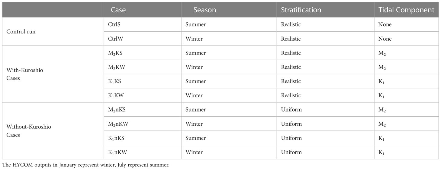
Table 1 Setup for each experiment.

For the cases with the Kuroshio (M₂KS, M₂KW, K₁KS, K₁KW in Table 1), our model setup is the same as the control run, except that the tidal forcing is now included. As the initial and boundary conditions for temperature, salinity, velocity and sea level from the HYCOM outputs are realistic, the initial density and stratification are horizontally non-uniform, and the initial velocity field contains the Kuroshio information (Figure S1 in the supplementary material). In contrast, for the cases without the Kuroshio (M₂nKS, M₂nKW, K₁nKS, K₁nKW in Table 1), the initial and boundary conditions for temperature and salinity is obtained by spatial averaging the HYCOM outputs over the LS region. Therefore, both the density and stratification are horizontally uniform (Figure S1 in the supplementary material). Such uniform stratification has been used in previous studies on internal tides (e.g., Kerry et al., 2013; Xu et al., 2016; Wang et al., 2018; Chang et al., 2019). It is noted that the inflow/outflow boundary condition is specified in the with-Kuroshio cases and excluded in the without-Kuroshio cases. Based on the thermal-wind relation, a horizontally uniform hydrography corresponds to an absence of vertical shear, i.e, an absence of baroclinic flow. In addition, in these model runs (M₂nKS, M₂nKW, K₁nKS, K₁nKW in Table 1), the initial velocity is set to zero, so the Kuroshio flow is absent and thus its effects on internal tides are effectively removed.

Each case in Table 1 is run for 15 days for the following reasons. First, a 15-day period is long enough to allow internal tides to propagate through the model domain and this integration time was also used in previous studies involving the SCS or the LS (Jan et al., 2008; Xu et al., 2016; Guo et al., 2020b). Second, the domain-averaged sea surface height (SSH) and kinetic energy time series indicate that our model solution has reached equilibrium in 15 days (not shown). An even longer time of model integration may lead to large deviations between the simulation and the initial states, in particular, for the experiments without wind forcing and data assimilation. A relatively short model run can help our model solution maintain a climatological steady state that is close to that in the HYCOM reanalysis. Such a realistic Kuroshio is important for evaluating the Kuroshio’s effect on the internal tides. Third, the Kuroshio intrusion into the SCS has different paths (Figure 1) and generally shows a seasonal pattern (Nan et al., 2011; Nan et al., 2015). However, the timescale of the dominant Kuroshio variability is O(100) days, and thus much longer than the timescale of internal tides (Zhang et al., 2001; Johns et al., 2001; Yin et al., 2017; Chang et al., 2019). Therefore, for the with-Kuroshio cases, we assume that the Kuroshio is quasi-steady and include the Kuroshio information in only the initial and boundary conditions. Using the quasi-steady setup can help us focusing on fundamental dynamics, making it easier to interpret the Kuroshio’s influence.

Our model setup has also been found useful in relevant previous studies. For example, to investigate the interaction between the M₂ internal tides and subtidal flow in Hawaii Ridge and the northeast of Taiwan, Zaron and Egbert (2014) and Chang et al. (2019) both used Simple Ocean Data Assimilation (SODA) ocean analysis data as the initial background field, and the models run for 14 and 30 days, respectively. Hsin et al. (2012) assessed the relative importance of open sea inflow/outflow, wind stress and surface heat flux in regulating Luzon Strait transport (LST) and its seasonality through several elimination model experiments. Their inflow/outflow at the open boundaries of the experiment NO was derived from the 10-year mean from North Pacific Ocean (NPO) model outputs, which is similar to our model settings of the with Kuroshio cases.

The change of Kuroshio invasion is related to the wind in the vicinity of the LS, such as the wind stress curl off southwest Taiwan (Wu and Hsin, 2012) and the East Asian monsoon (Hsin et al., 2012).But following Hsin et al. (2012); Jan et al. (2012) and Chang et al. (2019), wind forcing is not included in our experiments. The reasons are as follows. Winds can generate internal waves (Kitade and Matsuyama, 2000). Wind forcing can also influence the distribution and dissipation of internal tide energy (Hall and Davies, 2007; Masunaga et al., 2019). We avoid such added complexity here. Our current model setup without wind reduces the experiment to the simplest system, which allows us to focus on basic physics of the Kuroshio effect on internal tides. For the experiment NO in Hsin et al. (2012), the model runs are more stable in the absence of wind stress and heat flux forcing while fixing the open ocean inflows/outflows at the 10 year mean from NPO model.

2.2 Baroclinic tide energy equation

To assess the effects of background stratification, and thus the Kuroshio flow shear, on internal tides, we use the energy equation of the baroclinic tides from Song and Chen (2020). In this equation, the variable a is decomposed into a background mean state a^m and a perturbation component a':

$\begin{array}{ll}a(x,y,z,t)=a^m(x,y,z)+a^{\prime }(x,y,z,t).& (1)\end{array}$

For example, a can represent pressure p, density ρ, or velocity vector u. The perturbation component can be further decomposed into barotropic a^bt and baroclinic modes a^bc,

$\begin{array}{ll}{a}^{bt}=\frac{1}{\eta +H}{\displaystyle {\int }_{-H}^{\eta }{a}^{\prime }dz},a^{bc}=a^{\prime }-a^{bt}.& (2)\end{array}$

The variables η and H represent the ocean surface elevation and water depth, respectively. With this approach, the background field is described by the background mean-state variables (a^m) and assumed constant.

Using the above variable decomposition, one can obtain the time-and-depth-integrated nonlinear baroclinic tide energy equations as

$\begin{array}{ll}Tra{n}^{bc}+Conv-{\mathrm{Div}}^{\mathrm{bc}}={ϵ}^{bc},& (3)\end{array}$

where Tran^bc denotes the transfer of energy from the mean flow to the baroclinc tidal flow:

$\begin{array}{ll}Tra{n}^{bc}\text{= - }{\displaystyle {\int }_{-H}^{\eta }({\rho }_c{\mathit{u}}_h^{bc}{u}^{\prime })·\nabla {\mathit{u}}_h^{m}dz}.& (4)\end{array}$

Here ρ_c is the constant density and u_h means horizontal velocity vector. The term Tran^bc arises from the nonlinear interaction between the background shear and internal tides, and thus it is hereafter termed I_m-bc (Song and Chen, 2020). The next term Conv represents the total conversion rate of energy from barotropic to baroclinic tidal flow, hereafter called ‘total conversion rate’,

$\begin{array}{ll}Conv=Conv\_linear\underset{I_{bt-bc}}{\underbrace{-{\rho }_c{\displaystyle {\int }_{-H}^{\eta }(u_h^{bc}{\mathit{u}}_h)·({\nabla }_h{\mathit{u}}_h^{bt})dz}}},& (5)\end{array}$

where I_bt-bc arises from the nonlinearity of the system and is zero in the linear case (Song and Chen, 2020). The term Conv_linear represents the linear conversion rate,

$\begin{array}{ll}Conv\_linear=\frac{1}{2}{p^{\prime }}_{\theta A}(-H)w_{bt\theta A}(-H)\cos ({\theta }_{p^{\prime }}-{\theta }_{w_{bt}}).& (6)\end{array}$

Conv_linear has three factors: the amplitude of the pressure perturbation at the bottom p'_θA(-H), the vertical component of the barotropic flow w_btθA(-H), and the Greenwich phase difference cos(θp’-θ_Wbt)), where subscript A indicates amplitude. For the derivation of Eq. (6), see Zilberman et al. (2011), Kerry et al. (2013) and Kerry et al. (2014). The term Div^bc from Eq. (3) quantifies the divergence of the energy flux:

$\begin{array}{ll}Di{v}^{bc}={\nabla }_h·[\underset{F_{non}^{bc}}{\underbrace{{\displaystyle {\int }_{-H}^{\eta }{\mathit{u}}_h·(k{e}^{bc}+ape)dz}}}+{\displaystyle {\int }_{-H}^{\eta }{\mathit{u}}_h^{bc}{p}^{bc}dz}],& (7)\end{array}$

where F_non^bc represents the horizontal advection of local mechanical energy of internal tides (ke^bc + ape) by the background circulation. Finally, ε^bc the right side of Eq. (3), denotes the dissipation rate of internal tides. Compared to the energy equations in the linear system, the nonlinear energy equations have three additional terms: I_m-bc [Eq. (4)], I_bt-bc [Eq. (5)], and the horizontal divergence of F_non^bc which is part of Div^bc [Eq. (7)]. For details of the derivation, see Song and Chen (2020).

To diagnose the above energy terms, the horizontal tidal velocity u'_h, the density perturbation ρ', and the pressure perturbation ρ' are first filtered with a specific band to extract the semidiurnal (1.83-2.20 cpd) and diurnal (0.80-1.15 cpd) motions. Given the relatively low frequencies of the background flow, we use a low-pass filter with a cutoff frequency of 0.3 cpd to extract subtidal motion. As Eqs. (3) - (7) are based on the assumption that the background flow is steady, we assume that the simulated background state is constant over three days, so we use the last three days of model outputs for the energy diagnosis.

3 Model validation

3.1 Background state

In the background state, the simulated Kuroshio flows northward along the eastern side of the Philippines, crossing the Balintang Strait and then entering the SCS (Figure 2, top row). It is about 120 km wide, with maximum speeds of ~1.2 m s^-1 in winter and ~1.3 m s^-1 in summer, averaged over the upper 100 m of the 121°E meridional section (Figure 2, the bottom row). Part of the Kuroshio flows out along the southern part of Taiwan and then travels northward along the eastern part of Taiwan. Overall, the modeled flow agrees well with that from the SODA reanalysis data. The RMSEs (root mean square error) of the current speed for cases CtrlS and CtrlW are 0.15 m s^-1 and 0.16 m s^-1 in the whole domain, respectively. The probability that the modeled current direction differs from SODA by less than 60° is ~70%, with less than 35° being about 50%, indicating good agreement.

FIGURE 2

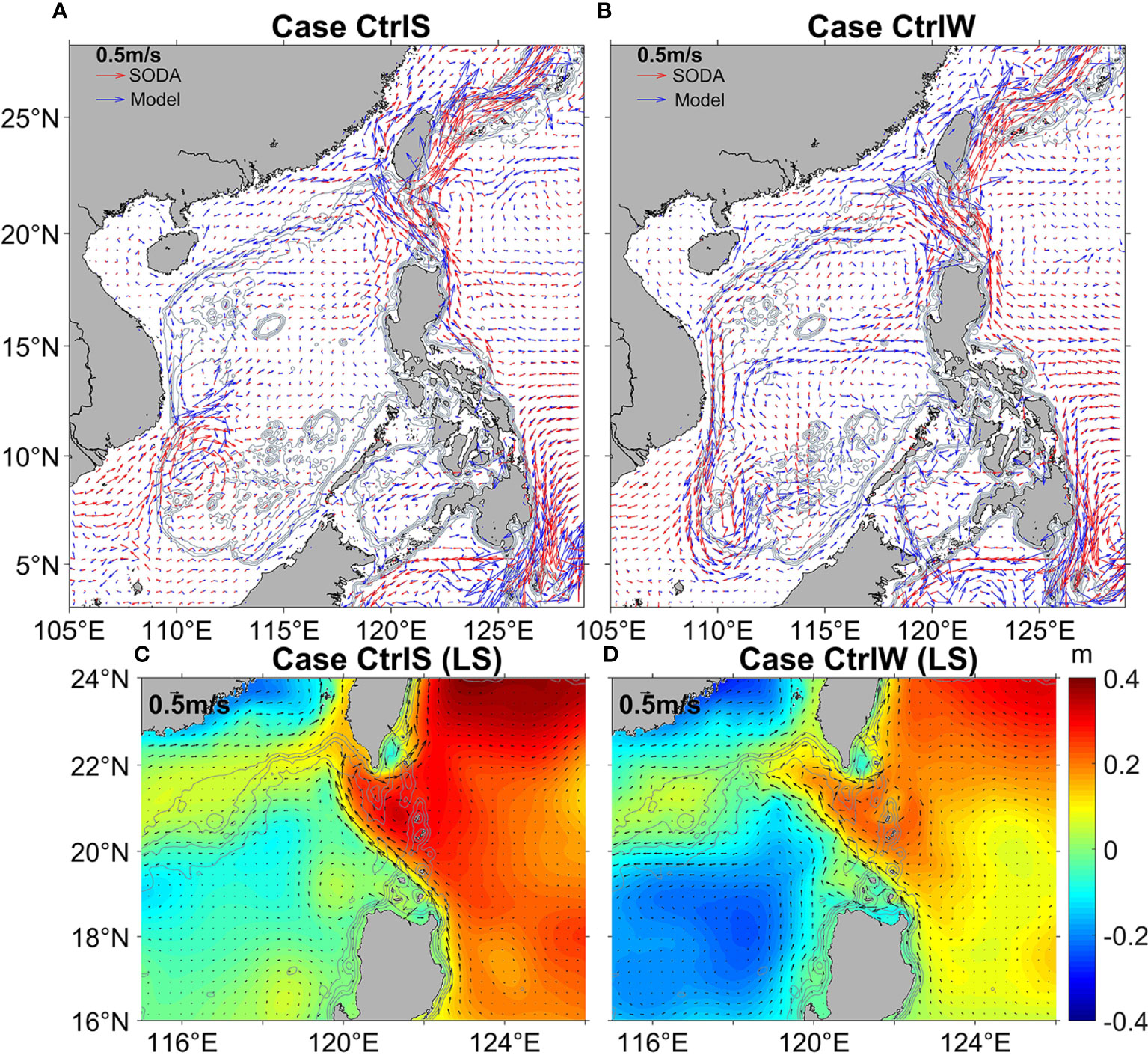
Figure 2 Mean flow vectors from the simulations and from the SODA (simple ocean data assimilation) reanalysis data. (A) Summer case CtrlS (blue), SODA (red). (B) Winter case CtrlW (blue), SODA (red). (C, D) show the mean velocity vector averaged over the upper 100 m and the sea surface height (color, m) from cases (C) CtrlS and (D) CtrlW in the LS region.

Concerning SSH, we find the results in Figures 2C, D to closely agree with the altimeter data in Nan et al. (2011) (not shown in the figure). Moreover, the difference between the maximum and minimum SSH values, for both the simulation and SODA reanalysis data, exceed 0.50 m, which is much greater than the RMSE values (0.08-0.09 m). Also, the correlation coefficients are greater than 0.84. Thus, the SSH also agrees well with SODA.

Concerning the three main Kuroshio paths into the SCS, the leaking path dominates in winter, the leaping path dominates in summer, and the looping path instead appears just southwest of Taiwan more frequently in winter than in other seasons (Wu and Chiang, 2007; Nan et al., 2015). Similarly, our simulation generally has the leaking path in summer and the looping path in winter (Figures 2C, D). Overall, the simulated Kuroshio velocities and paths appear reasonable.

Our model also reasonably captures the background hydrographic fields. For example, the meridional cross-sections of temperature and salinity at 120.75°E agree well with those from WOA18 (Figure 3). The RMSEs of temperature for cases CtrlS and CtrlW are both less than 1, and the RMSEs of salt are both less than 0.2, with the correlation coefficients of temperature exceeding 99%. In addition, for both WOA18 and our model solution, the isotherms in the LS region tilt toward the east (the Philippine Sea) (not shown).

FIGURE 3

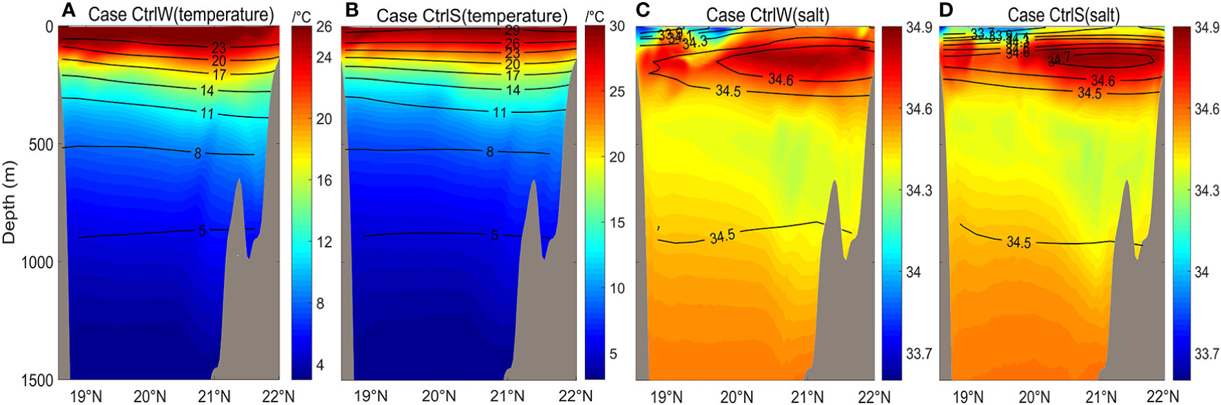
Figure 3 Simulated temperature and salinity profiles at 120.75°E, 18.5°N-22°N (blue line section in Figure 1) overlaid with WOA18 (world ocean database) annual mean data within the upper 1500 m. (A) Simulated temperature profile of winter case in color, with WOA18 temperatures as black contours. (B) Same as (A) except summer. (C) Same as (A) except salinity profile in winter. (D) Same as (C) except summer.

3.2 Barotropic tides

Using the harmonic analysis method from Pawlowicz et al. (2002), we obtained the cotidal charts of M₂ and K₁ tides from the last three days of modelling outputs. In Figure 4, we compare the simulated results to the TPXO9 dataset. The distribution of simulated surface elevation and cophase lines are generally consistent with TPXO9, except that the simulated amplitude is slightly larger than TPXO9 near the shelf region. Small-scale fluctuations of the cophase lines occur in the LS and SCS regions, and these are mainly caused by the baroclinic tide signals (Niwa and Hibiya, 2004; Xu et al., 2016). Consistent with the altimetric estimates from Zhao (2014), the horizontal wavelength of M₂ and K₁ internal tides in our simulation, inferred from these fluctuations, are about 160 and 320 km, respectively. The RMSEs of the amplitudes are 11.70 and 6.95 cm, respectively for cases M₂KS and K₁KS, and the correlation coefficients of the amplitudes exceed 92% with a confidence level of 95%. Here, we further calculate a new RMSE specifically for tides in another way. Following Cummins and Oey (1997),

FIGURE 4

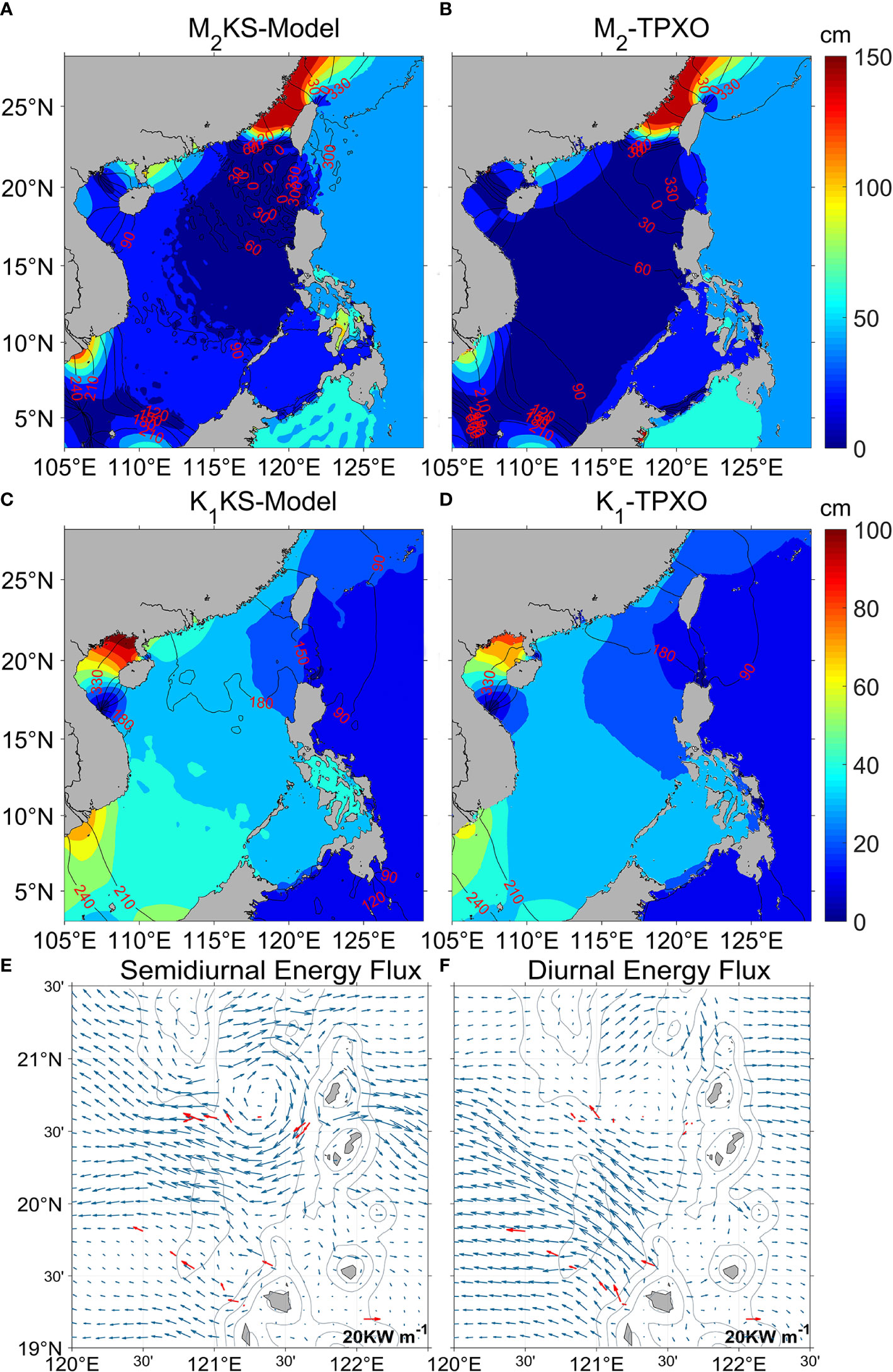
Figure 4 Modeled and observed cotidal chart and baroclinic energy flux. (A) Cotidal for case M₂KS. Color indicates amplitudes (cm) and black contours give the cophase lines (degree). (B) M₂ from TPXO9 observations. (C) Cotidal chart for case K₁KS. (D) K₁ of TPXO9. (E) Baroclinic energy flux from in situ observations (red, Alford et al., 2011) and our experiment forced by semidiurnal (M₂ and S₂) tide (blue). (F) The same as (E) but for diurnal (K₁ and O₁) tide.

$\begin{array}{ll}RMSE=\sqrt{\frac{1}{2}(A_o^2+A_m^2)-A_o{A}_m\cos ({\varphi }_o-{\varphi }_m)},& (8)\end{array}$

where A and ϕ represent the amplitudes and phases of the surface elevations. The subscripts o and m refer the results from TPXO9 and our model, respectively. The new mean RMSEs (calculated using Eq. 8) of the eight cases (M₂KS, M₂KW, M₂nKS, M₂nKW, K₁KS, K₁KW, K₁nKS and K₁nKW) are 4.50, 5.03, 4.58, 5.39, 4.34, 4.35, 4.37, and 4.38 cm, respectively.

3.3 Baroclinic tides

To assess our model fidelity on internal tides, we ran additional experiments that include semidiurnal tides (M₂ and S₂) and diurnal tides (K₁ and O₁) at the open boundaries. Results in Figures 4E, F show that the simulations well capture the propagation pattern of internal tides. For both diurnal and semidiurnal tides, the simulated energy-flux directions agree with observations from Alford et al. (2011). The energy-flux magnitudes also agree with observations, particularly in the region south of 20°N. We provide further statistics in Table 2. In the semidiurnal case, the simulated maximum energy flux is 55.2 kW m^-1 in the LS region (120°E-122.5°E, 19°N-21.5°N), which is much greater than the energy flux RMSE of 9.1 kW m^-1, and the average energy flux is 15.3 kW m^-1 (Table 2). The RMSE of the energy-flux direction is no more than 23.5°. In the diurnal case, the RMSE of energy flux is 7.1 kW m^-1, and that of the energy-flux direction is 32.5°. By including all semidiurnal tidal components in our simulation, smaller deviations would likely be obtained.

TABLE 2

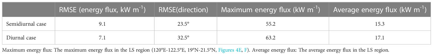
Table 2 The RMSEs between internal tide energy flux of the simulations and that of the estimate from in situ observations (Alford et al., 2011).

4 Effects of the Kuroshio on internal tides

4.1 Internal tides in the case with the Kuroshio

In the simulations with the Kuroshio, the internal tide energy flux and conversion rate are spatially heterogeneous. Figure 5 shows that the dominant generation site of internal tides is in the LS region. Here, the M₂ tide generates energy of ~17.1 GW (case M₂KS), whereas K₁ generates ~10.6 GW (case K₁KS). As marked by the light blue arrows in Figure 5A, there are three M₂ energy beams radiating from the LS: one points to the northeastern shelf of the SCS (northern beam), another directs southwest to the deep-sea basin (southern beam), and the third one east to the Pacific Ocean. This three-beam pattern is generally consistent with previous observational and modelling studies (Kerry et al., 2013; Zhao, 2014; Xu et al., 2016). The northern beam heads northwestward, converging near the Dongsha Islands, and then dissipating at the continental slope. The southern beam, much weaker than the northern beam, propagates southwestward, crossing the deep-sea basin, and then traveling for more than 1000 km to reach the Vietnam coast or the Nansha Islands due to its small dissipation rate. For the K₁ internal tides, two main beams radiate from the LS: one points southwest to the deep-sea basin of the SCS and the other points east to the Pacific (Figure 5B). The complex wave forms and propagation paths of internal tides radiating from the LS into SCS may be due to the impact of rotation, complex topography, and the mutual interference with locally generated internal tides.

FIGURE 5

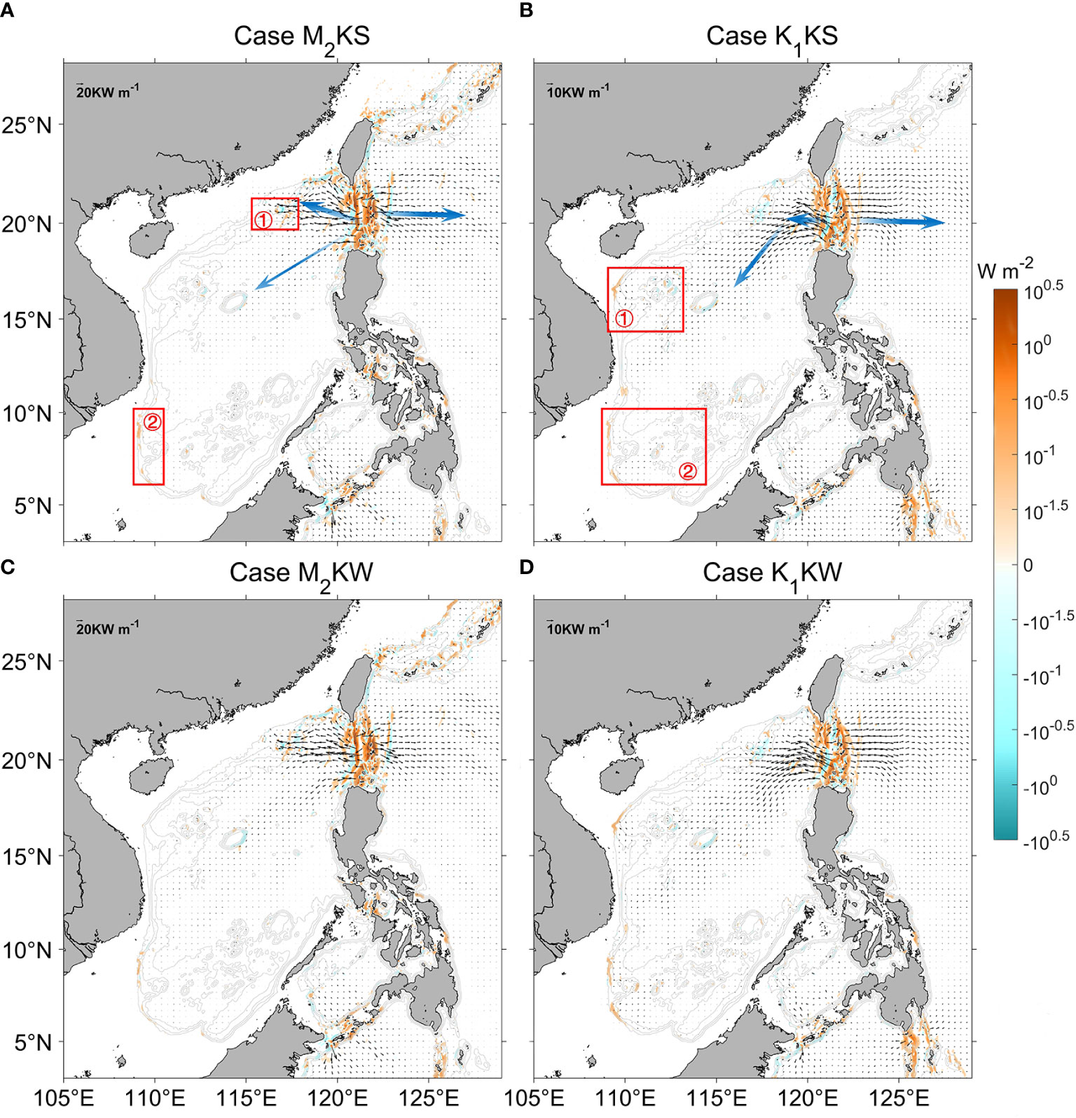
Figure 5 Modeled depth-integrated and period-averaged internal tide energy flux (black arrows, kW m^-1) and conversion rate (color, W m^-2) for with-Kuroshio cases. (A) Case M₂KS. Gray contours are isobaths. Blue arrows indicate energy beams. Red boxes marked ① and ② show the main areas of internal tide generation within the SCS. (B) Case K₁KS. (C) Case M₂KW. (D) Case K₁KW.

Besides the LS region, local generation sites of internal tides occur within the SCS. The strength of generation of these internal tides is controlled by both the topographic slope and the strength of barotropic tides. Also, the strength distribution of the K₁ barotropic tides differs from that of M₂ (Figure 4). Consequently, the generation sites of M₂ internal tides differ from those of K₁ within the SCS. In particular, the generation of M₂ lies mainly at the northeastern continental slope (box “1” in Figure 5A) and the southwestern continental slope (box “2”), whereas those for K₁ are similarly marked in Figure 5B, being around the Xisha Islands and the northwestern continental slope (“1”), and around the Nansha Islands and the southwestern continental slope (“2”). As shown in Zu et al. (2008), this difference is due to the fact that the energy flux intensities of the two barotropic tidal components vary in different regions within the SCS.

The seasonality of internal tides can be evaluated by comparing the summer cases in the top row of Figure 5 to the winter cases in the bottom row. In this realistic stratification scenario, the source and propagation direction of the tides in the SCS vary little from season to season. However, as shown in the next section, the energy magnitude undergoes a significant seasonal cycle.

4.2 Effects of the Kuroshio on conversion rates and baroclinic energy fluxes

4.2.1 M₂ internal tides

Results show that modulation of the double-ridge system complicate the generation and propagation of internal tides in the LS. For case M₂KS (with-Kuroshio, summer), Figure 6A shows the baroclinic energy flux and conversion rate. We examine the five main M₂ internal tide-generating sites (labeled). Conversion rates at sites 2, 4, and 5 are significantly higher than those at 1 and 3 due to a larger topographic criticality there (Kerry et al., 2013). Sites 1 and 4 are the main sources of the ‘northern beam’, site 3 is the main source of the ‘southern beam’, and site 5 is the main generation site of internal tides propagating into the Pacific Ocean. The strongest energy flux is about 60 kW m^-1, propagating northwestward from just south of site 2. Despite the higher conversion rates at site 2, only a small portion of energy generated here crosses the high Lanyu ridge into the Pacific Ocean due to a topographic blocking effect.

FIGURE 6

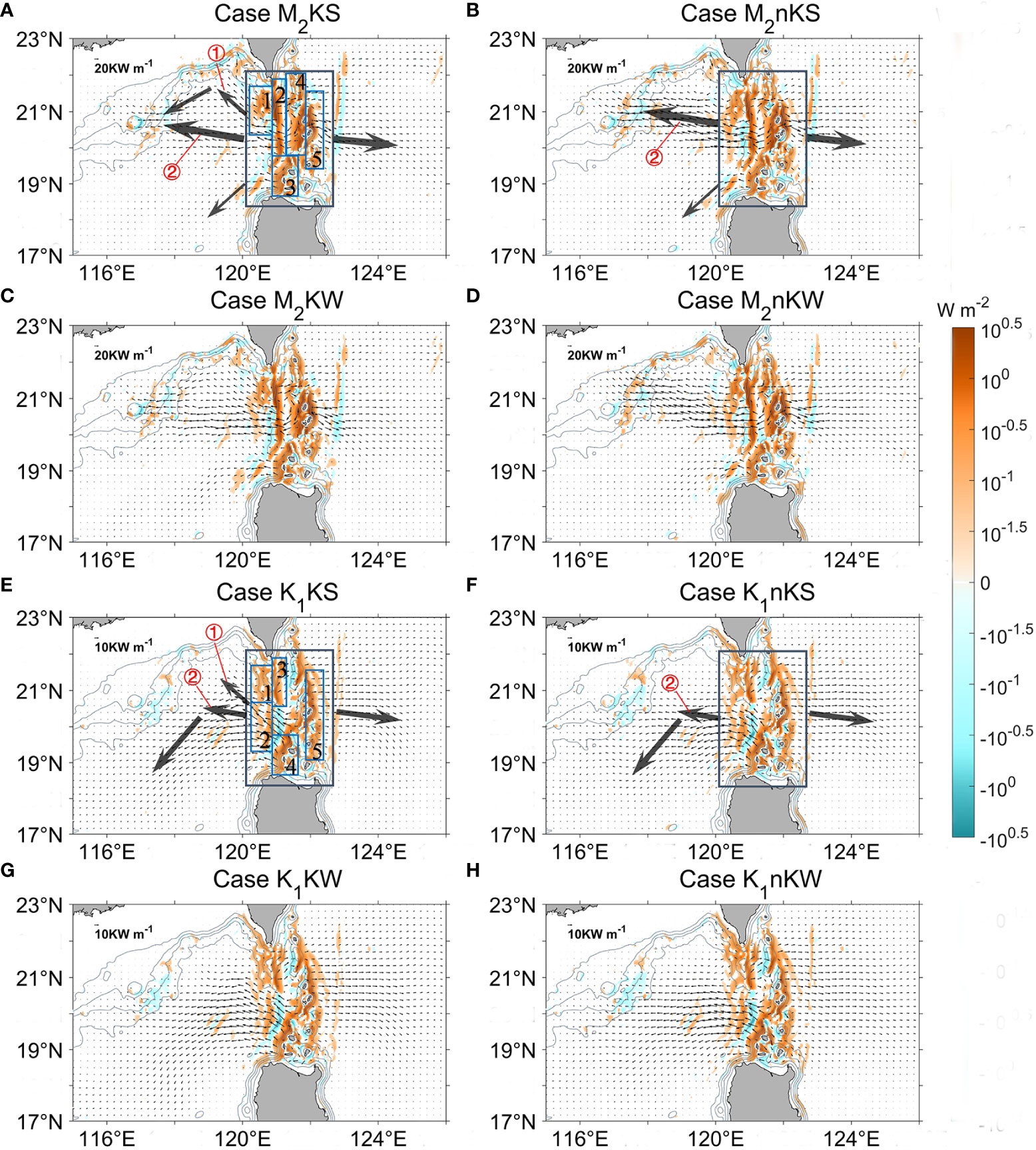
Figure 6 Modeled baroclinic energy flux (thin black arrows) and conversion rate (color) of the M₂ and K₁ internal tides in the LS and nearby regions. (A–D) For M₂ internal tides. Top row is summer, second row is winter. Left column is the with-Kuroshio cases, right is the without-Kuroshio cases. The gray boxes outline the LS region (120°E - 122.5°E, 18.3° N - 22° N). The blue boxes in the large gray boxes indicate the five M₂ subregions discussed in the main text. The thick black arrows show the main direction of internal tide energy from the source of the LS. Red circles ① and ② represent the northwestward and westward internal tide energy flux, respectively. (E–H) The same as (A–D), but for K₁ internal tides.

West of the LS, the conversion rate near the Dongsha Islands (118°E, 20.75°N) is negative (Figure 6A). In general, negative values occur due to the phase differences between local- and remote-generated baroclinic tides, indicating the presence of multiple source sites (Zilberman et al., 2009; Hall and Carter, 2011; Carter et al., 2012). Here, the negative conversion rate indicates that remote signals from the LS modulate internal tides in the eastern part of the Dongsha Plateau. Therefore, the Dongsha Islands are an important convergence region for the M₂ internal tides.

For the with- and without-Kuroshio cases, the areas of the internal tide energy generation are similar in the LS, and the Kuroshio does not notably impact the source of the internal tides. However, the Kuroshio does affect the pattern of baroclinic energy fluxes. Specifically, the with-Kuroshio case shows a noticeable portion of internal tide energy from the LS that radiates northwestward onto the continental slope (Figure 6A, ①), whereas the without-Kuroshio case instead has a dominant energy radiation direction that is westward (Figure 6B, ②). Therefore, compared to case M₂nKS, the with-Kuroshio case M₂KS shows much less far-distant propagating energy within the SCS. In case M₂nKS, the energy propagating to the Dongsha Plateau exceeds that of M₂KS, and most internal tides pass the north part of the Dongsha Islands. In case M₂KS, however, the Dongsha Islands is a region where internal tides converge.

In winter, for both the with-Kuroshio (Figure 6C) and without-Kuroshio (Figure 6D) cases, the dominant energy fluxes are zonally directed westward into the SCS. However, a northwestward radiation of energy from the LS occurs in the with-Kuroshio case, but not in the without-Kuroshio case. The width and direction of these northwestward-propagating tides resemble those of the Kuroshio flow, with both showing seasonal variations (Figures 2C, D). However, in the without-Kuroshio case, the dominant energy radiation directions, which are approximately zonal, are less affected by the seasons. Therefore, the with-Kuroshio case shows greater seasonal variations in the direction of tidal energy flux in the LS than in the without-Kuroshio case, especially for the northwestward internal tides under the influence of the Kuroshio.

4.2.2 K₁ internal tides

As was the case for the M₂ tides, the K₁ internal tides have five main generation sites in the with-Kuroshio case in summer. Figure 6E shows that sites 2 and 4 are the main generation areas of internal tides propagating westward into the SCS. The K₁ internal tides generated at site 3 propagate eastward, but are blocked by the northern part of the high Lanyu Ridge. As a result, site 5 is the most important source of eastward-propagating tides into the Pacific, showing relatively uniform radiation along the entire ridge. Similar to that of case M₂KS, the Dongsha Plateau is an important convergence area of K₁ internal tides, as revealed by the negative conversion rates there.

In summer, although their generation sites of internal tides are similar, the baroclinic energy flux directions without the Kuroshio differ from those with the Kuroshio (Figures 6E, F). On the SCS side, the with-Kuroshio case has both northwestward- (Figure 6E, ①) and westward-propagating (Figure 6E, ②) internal tides, whereas the without-Kuroshio case is dominated by westward internal tides (Figure 6F, ②). On the Pacific side, the dominant energy radiating direction is eastward for both the with- and without-Kuroshio cases. In winter, the effect of the Kuroshio on the energy radiation direction is similar to that in summer. However, the contrast between the two cases is less significant than that in summer (Figures 6G, H).

4.3 Effects of the Kuroshio on nonlinear energy terms

In the nonlinear case, there is energy exchange between the background shear and internal tides. The corresponding energy exchange rate I_m-bc can be quantified using Eq. (4). Overall, the magnitude of I_m-bc is only about 1-10% of the magnitude of the total conversion rate (Conv). Considering the spatial pattern of I_m-bc in summer, both its peak magnitude and extent are larger in the with-Kuroshio case than those in the without-Kuroshio case (Figure 7). The tidal current can be generated by tidal forcing from the open boundary, which produces relatively weak background flow in the absence of Kuroshio. This weak background flow contributes a relatively small energy exchange rate between the background state and the internal tides (Figure S2 in the supplementary material).

FIGURE 7

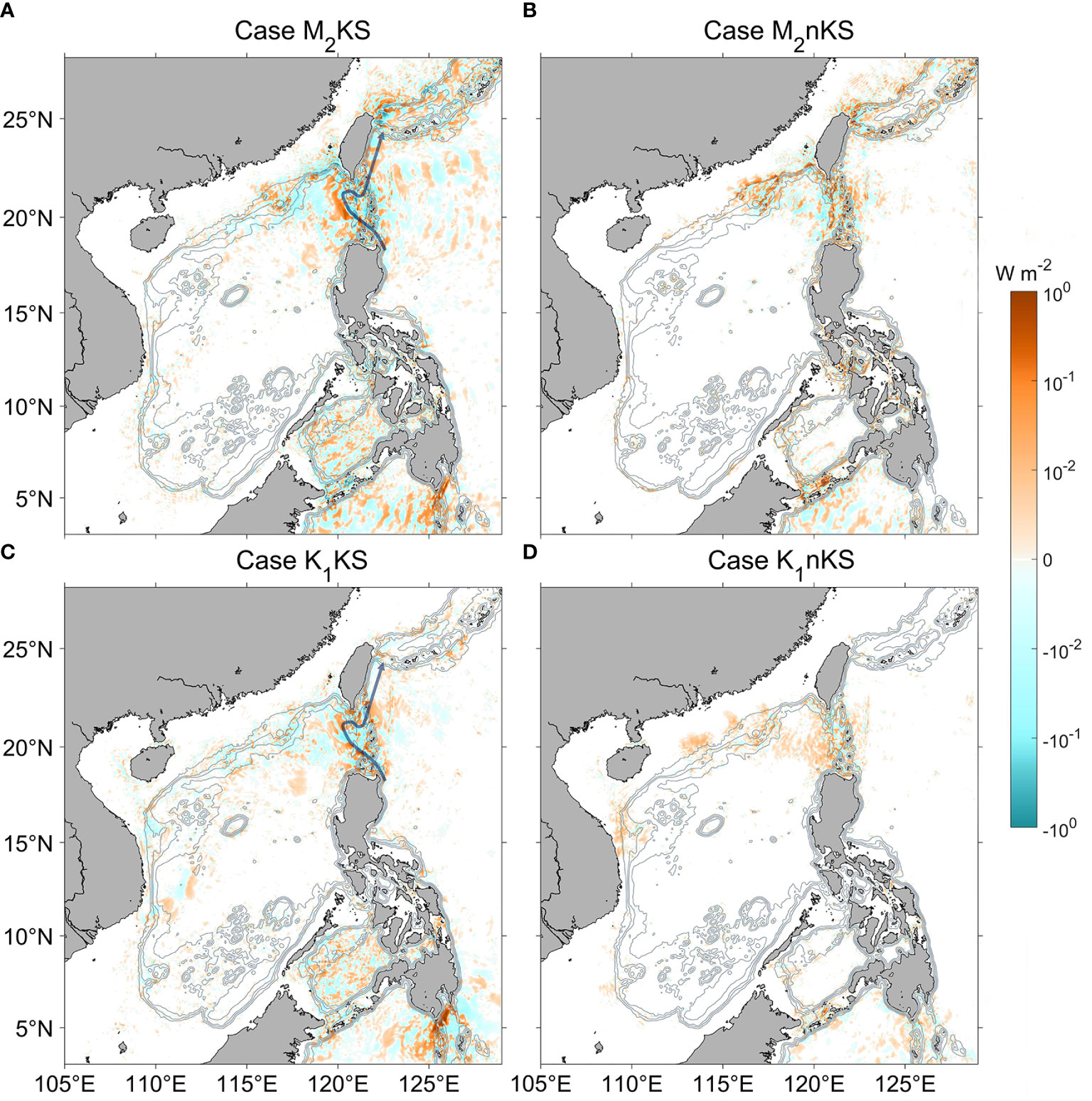
Figure 7 Distribution of I_m-bc (color, W m^-2) for four summer cases. (A) M₂KS. Gray contours indicate isobaths. The blue line shows the Kuroshio path during the simulation period. (B) M₂nKS. (C) K₁KS. (D) K₁nKS. Left column is with-Kuroshio, right without.

Consider the horizontal shear Shear_H and vertical shear Shear_v:

$\begin{array}{ll}Shea{r}_H=\sqrt{{\left(\frac{du}{dx}\right)}^2+{\left(\frac{du}{dy}\right)}^2+{\left(\frac{dv}{dx}\right)}^2+{\left(\frac{dv}{dy}\right)}^2}& (9)\end{array}$

$\begin{array}{ll}shea{r}_V=\sqrt{{\left(\frac{du}{dz}\right)}^2+{\left(\frac{dv}{dz}\right)}^2}& (10)\end{array}$

The distributions of Shear_H and Shear_V for cases M₂KS and M₂nKS are shown in Figure 8. In the with-Kuroshio case, the Shear_H at 100 m depth along the Kuroshio path typically exceeds 1 × 10^-5 s^-1 (Figure 8A). In the without-Kuroshio case, the Shear_H is generally less than 1 × 10^-5 s^-1 over the whole region (Figure 8B). For the Shear_v, the large values are also mainly distributed along the path of the Kuroshio, and the magnitude for the without-Kuroshio case is much smaller over the whole region (Figures 8C, D). In general, the notable background shear is mainly distributed along the Kuroshio path.

FIGURE 8

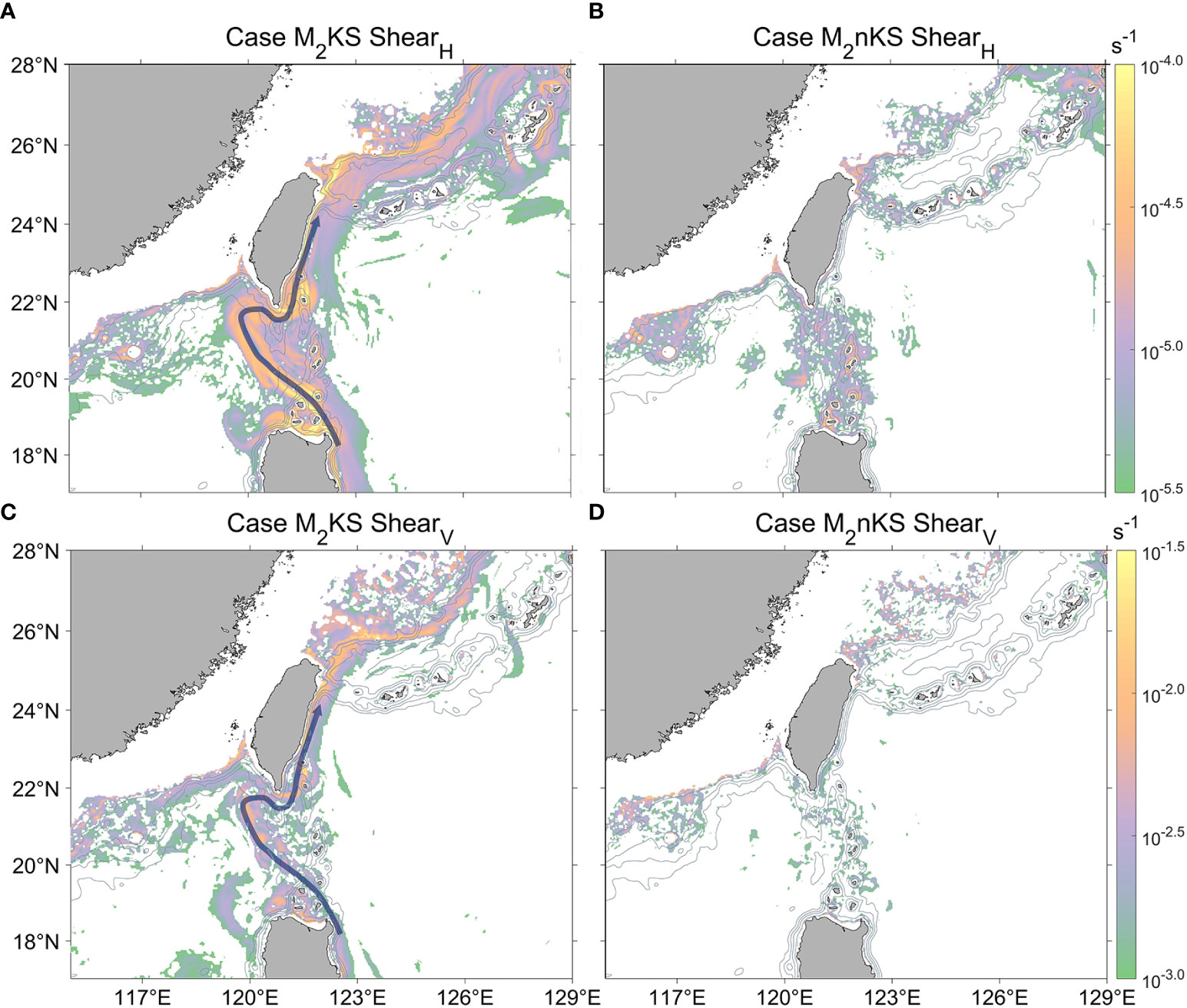
Figure 8 Distribution of Shear_H and Shear_v (color, s^-1) at 100 m depth for two summer cases (M₂KS and M₂nKS). The curved path represents the Kuroshio path. The top row (A, B) is Shear_H, and the bottom row (C, D) is Shear_v. The left column (A, C) gives the with-Kuroshio case (M₂KS), and the right column (B, D) shows the without-Kuroshio case (M₂nKS). Gray contours indicate the isobaths.

The energy exchange I_m-bc in Figure 7 is large in the regions where both the background shear (Figure 8) and internal tide energy (Figure 5) are large. For the M₂KS case (Figure 7A), the magnitude of I_m-bc in the LS region is about 10^-2 - 10⁰ W m^-2, which is 1-2 orders of magnitude larger than that in the open ocean (about 10^-2 W m^-2). Along the Kuroshio path (e.g., Hengchun Ridge and northeastern Taiwan), both the background shear and internal tide generation are intense, corresponding to a large I_m-bc. For case K₁KS (Figure 7C), elevated values of I_m-bc mainly occur in the LS region. As the continental slope near northeast Taiwan is not the main generation region of the K₁ internal tides, the magnitude of I_m-bc is small.

Besides the nonlinear interaction between the background shear and internal tides, there is also nonlinear interaction between barotropic and baroclinic tides (Section 2.2). The term I_bt-bc from Eq. (5) represents the energy exchange rate between barotropic and baroclinic tides. Compared to I_m-bc, large values of I_bt-bc cover a smaller area (Figures 9A-C). For case M₂KS, I_bt-bcis large in areas with prominent topography features, namely the East China Sea continental slope northeast of Taiwan and the two ridges of the LS (the Dongsha Plateau and the Ryukyu Ridge) (Figure 9A). In case M₂KS, I_bt-bc is also large along the Kuroshio path, especially in the southern part of the Hengchun and Lanyu ridges. For case K₁KS, however, the area with elevated values of I_bt-bc is smaller than that of case M₂KS, mainly along the two ridges of the LS (Figure 9C).

FIGURE 9

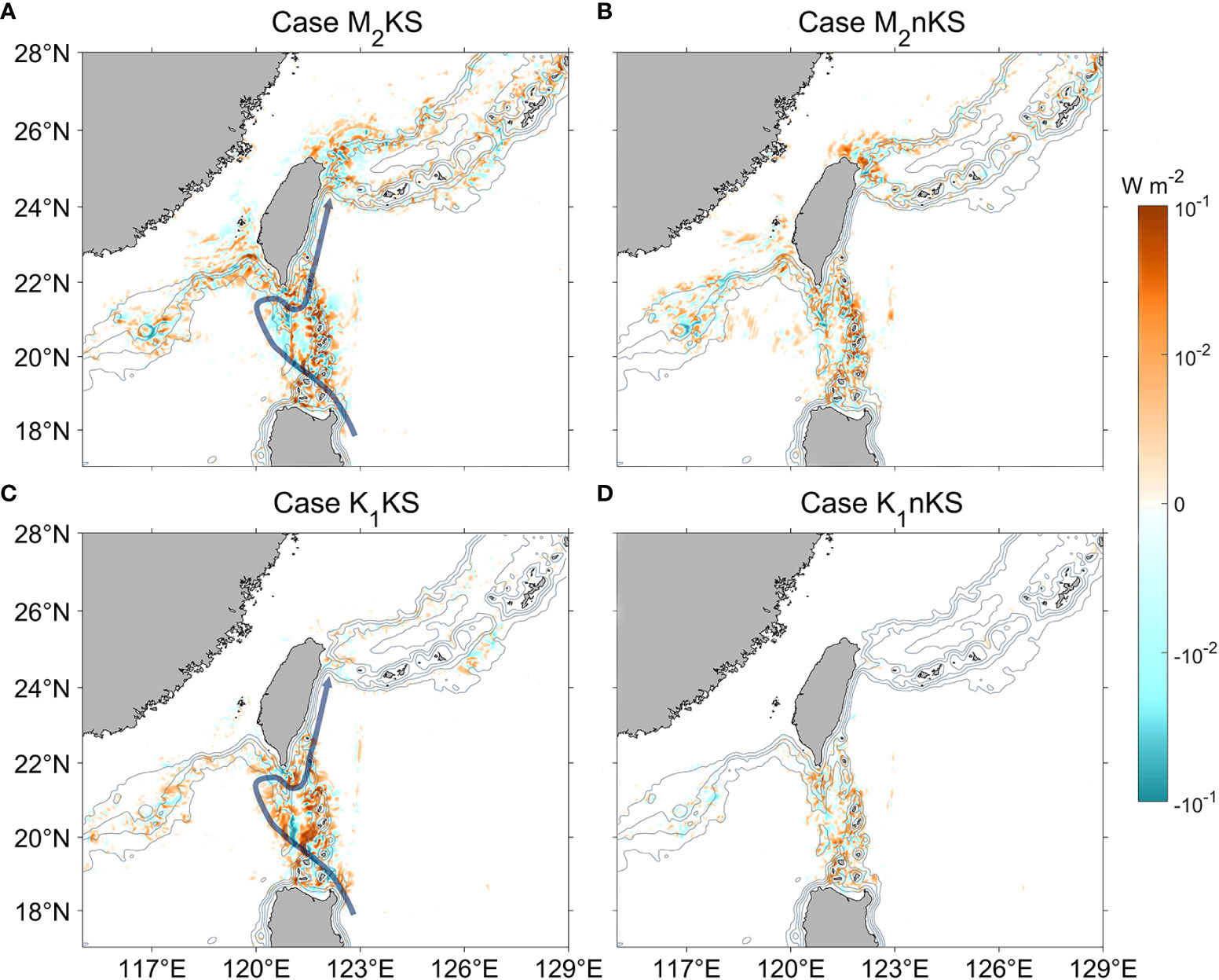
Figure 9 Distribution of Ibt-bc (color, W m-2) for four summer cases. (A) M2KS. Gray contours indicate isobaths. The blue line shows the Kuroshio path during the simulation period. (B) M2nKS. (C) K1KS. (D) K1nKS. Left column is with-Kuroshio, right without.

For case M₂KS, the magnitude of I_bt-bc is only about 10^-3-10^-1 W m^-2 in the LS region, much smaller than the total conversion rate, and even much smaller than I_m-bc. Therefore, I_bt-bc is a negligible nonlinear energy term in this case. Nevertheless, it can shed light on the source of internal tides and the Kuroshio effect. For both M₂ and K₁ internal tides, the magnitudes of I_bt-bc in the without-Kuroshio case are much smaller than those in the with-Kuroshio case (Figure 9), indicating that the Kuroshio tends to promote the interaction between barotropic and baroclinic tides. This sensitivity of I_bt-bc to the Kuroshio may be related to baroclinic tide generation. In particular, baroclinic internal tides can be generated when the background flow with temporal variability at tidal frequency passes a topography obstacle (e.g., a seamount or ridge). In the without-Kuroshio case, weak background flow shear probably corresponds to weak flow on topography. The weak flow decreases the energy exchange rate between barotropic and baroclinic tides and weakens the baroclinic internal tide.

In the baroclinic tide energy equation, the divergence of energy flux is induced by two processes: the advection of tide energy by background flow and the work done by pressure [Eq. (7)]. The contribution from advection is represented by the nonlinear term F_non^bc in Eq. (7). Representative results are shown in Figure 10. For the with-Kuroshio cases in summer (M₂KS and K₁KS, Figures 10A, B), the F_non^bc flux is largest in the LS, where it points northwestward and crosses the Hengchun Ridge to the SCS. Then, in winter (M₂KW), the F_non^bc flux is slightly stronger than in summer, directing northwestward and converging in the Dongsha Plateau (Figure 10C). The flux pattern here is similar to the leaking path of the Kuroshio (Figure 1), indicating that the contribution of the Kuroshio to F_non^bc is important for the with-Kuroshio case. For the M₂nKS case (Figure 10D), which does not include the Kuroshio, the maximum energy flux is only ~3 kW m^-1. It is much smaller than the maximum value of ~15 kW m^-1 for the with-Kuroshio cases shown in Figures 10A-C. The direction of the F_non^bc flux seems random, with little resemblance to the Kuroshio path. The small value of energy flux in the without-Kuroshio case arises from weak background flow near the LS.

FIGURE 10

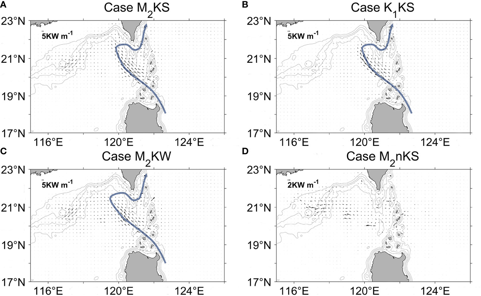
Figure 10 Spatial distribution of F_non^bc (vectors) in the LS for four cases. (A) M₂KS (summer, with-Kuroshio). Gray contours indicate isobaths. The curved path represents the Kuroshio path. (B) K₁KS (summer, with-Kuroshio). (C) M₂KW (winter, with-Kuroshio). (D) M₂nKS (summer, without-Kuroshio).

4.4 Energy budget in the Luzon Strait

4.4.1 Comparison with literature

We now consider the internal tide energy’s total conversion rate in the LS. Seasonally, the total conversion rate within the LS varies significantly. Consistent with Guo et al. (2020b), the rate here in winter is larger than that in summer. Specifically, the total conversion rate from M₂KW is about 3.2% higher than M₂KS, whereas M₂nKW is 2.6% higher than M₂nKS (Table 3). Similarly, that from K₁KW is about 5.5% higher than K₁KS, and K₁nKW 5.7% higher than K₁nKS. Note that the total conversion rate of M₂ here is comparable to the estimate from Alford et al. (2015); Xu et al. (2016), and Guo et al. (2020b). However, it is larger than that from Niwa and Hibiya (2004); Jan et al. (2008), and Kerry et al. (2013). In all of experiments listed in Table 3, the ratio between the local dissipation rate and the total conversion rate is roughly 30%. This number is close to the estimate by Kerry et al. (2013) of 33%, but it is slightly lower than that from Alford et al. (2011). The disagreement may come from the stratification conditions, mesh resolution, terrain smoothing method, and the choice of subgrid parameterization schemes.

TABLE 3

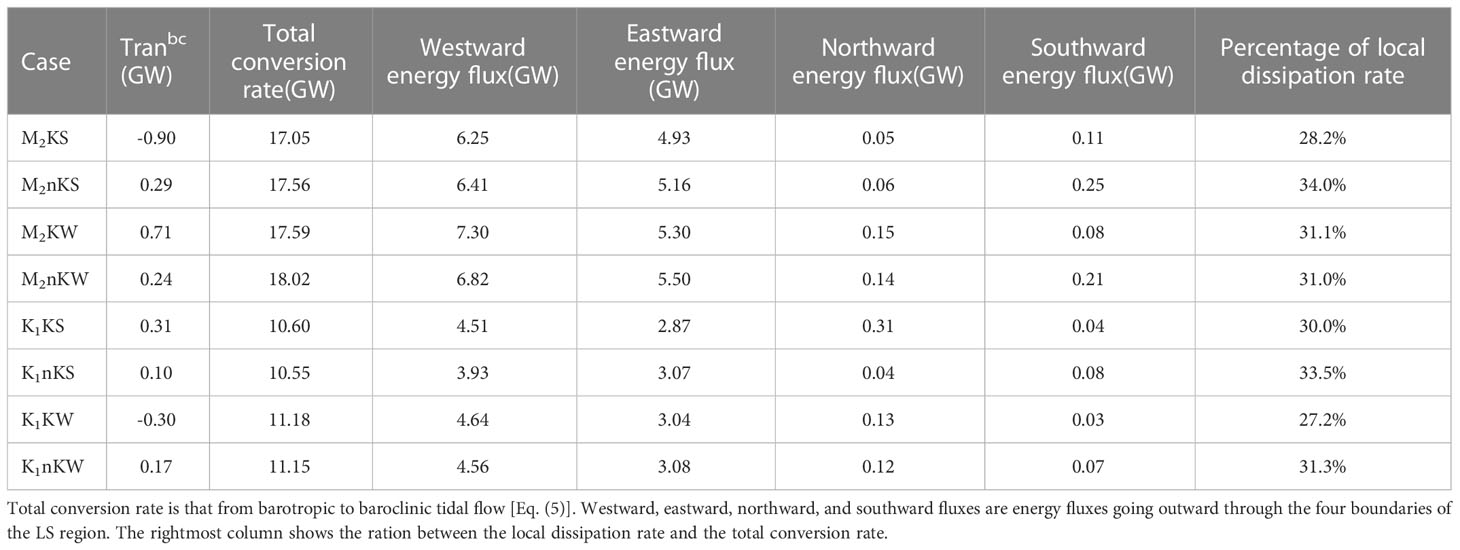
Table 3 The internal tide energy budget in the LS region (gray box, Figure 6A).

4.4.2 Energy fluxes

The content in Table 3 indicates that the response of the total conversion rate and local dissipation rate to the Kuroshio is small. However, the Kuroshio significantly affects the meridional energy fluxes radiating out of the LS. For example, the southward energy fluxes in M₂nKS is over twice that M₂KS, the same holding for M₂nKW over M₂KW as well as K₁KW over K₁nKW. Thus, removing the Kuroshio increases the southward energy fluxes in these cases. As to K₁KS and K₁nKS, removing the Kuroshio significantly decreases the northward energy fluxes going out of the LS. Compared to the K₁ experiments, both the westward and eastward energy fluxes in the M₂ experiments are larger (Table 3).

The internal tides propagating into the SCS are larger than that radiating into the Pacific Ocean. The energy flux patterns in Figure 6 show that the northward propagating internal tides are stronger in the with-Kuroshio case than those in the without-Kuroshio case. However, the direction of propagation to the Pacific differs little between the two cases. In other words, the propagation direction to the Pacific is less sensitive to the existence of the Kuroshio than that into the SCS.

4.4.3 Total conversion rate

We now consider how the Kuroshio influences the total energy conversion rate within the LS. Table 3 shows that the magnitude of Tran^bc in the with-Kuroshio case exceeds that of the without-Kuroshio case. For the with-Kuroshio case, Tran^bc accounts for about 2-6% of the total conversion rate, but only about 1-2% for the without-Kuroshio case. For the M₂ experiments, the total conversion rate for the with-Kuroshio case is smaller than that without the Kuroshio. For the K₁ experiments, however, the ratio of the total conversion rate between the with- and without-Kuroshio cases is nearly the same. This means that the K₁ case is less sensitive to the background condition than that for the M₂ case. For both with- and without-Kuroshio cases, the total conversion rate within the LS for the M₂ experiments are larger than those for the K₁ experiments. In general, the response of the total conversion rate to the Kuroshio is less than its seasonal variation.

We now examine the factors regulating the total conversion rate using Eqs. (5) and (6). As the nonlinear conversion rate from Eq. (5) is negligibly small, the total conversion rate Conv roughly equals Conv_linear. According Eq. (6), Conv_linear is determined by three factors: the bottom pressure perturbation p'_θA(-H), the vertical component of the barotropic flow w_btθA(-H) or w_bt for short, and the phase difference cos(θ_p'-θ_Wbt) between w_bt and the pressure perturbation, or just ‘phase difference’. The role of these variables in regulating internal tides has been previously discussed. For example, Kelly and Nash (2010) showed that the remotely generated internal tides can increase or decrease the local generation of internal tides, depending on the phase of the barotropic tides and the bottom pressure perturbation induced by the internal tides. Kerry et al. (2013) later found that in the LS and Mariana Island Arc, distant internal tides affect the conversion between barotropic and baroclinic tides by varying the amplitude of the bottom pressure disturbances in a complex pattern of spatial variability.

To evaluate the relative importance of the three factors in regulating the conversion rate response to the Kuroshio, we first examine the ratio of the three factors for the with-to-without Kuroshio cases (e.g., K₁KS vs. K₁nKS, M₂KW vs. M₂nKW). In Table 4, we show the Pearson correlation coefficients between the conversion rate ratio and the pressure perturbation ratio (the second column). The same is shown for the other two factors in the next two columns.

TABLE 4

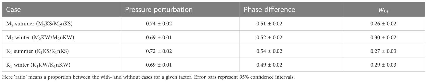
Table 4 Pearson correlation coefficients between the conversion rate ratio and the three factors listed in the column headings.

In both winter and summer, and for both M₂ and K₁, the Pearson correlation coefficient between the conversion rate ratio and the bottom pressure perturbation ratio is approximately 0.7, whereas the correlation coefficient for the phase difference is smaller, at about 0.5. The correlation between the conversion rate ratio and w_bt is the smallest, ranging from 0.26 to 0.30. Nevertheless, all the correlation coefficients from Table 4 are significant at the 95% confidence level, indicating that the three factors from Eq. (6) jointly determine the conversion ratio between the with- and without-Kuroshio cases. However, the effect of both the phase difference and the term w_bt on the conversion rate ratio is smaller than that of the bottom pressure perturbation. This perturbation may result from tide-topography interactions (Simmons et al., 2004). In addition, the isopycnal displacement caused by the warmer and saltier Kuroshio flow is another factor impacting the pressure perturbation (Jan et al., 2012). Our results suggest that the Kuroshio significantly modulates the tide-topography interaction process at the ocean bottom.

5 Summary and conclusion

This study used high-resolution ocean numerical simulations to evaluate the effects of the Kuroshio on the generation, propagation, and energy budget of internal tides in the LS. To detect the Kuroshio effect, we compare model results between two stratification scenarios: one adopts realistic stratification as the initial condition, the other with uniform stratification. The uniform stratification case was introduced to effectively remove the background flow shear and thus remove the Kuroshio intrusion effect. Then, we considered winter and summer experiments separately. To avoid the nonlinear interaction between multiple tidal components, each simulation case shown in Table 1 is only driven by one of two tidal forcings (M₂ or K₁) at the open boundaries.

For cases with- or without-Kuroshio, the dominant generation site of internal tides was always the LS region. However, there were significant differences between the with- and without-Kuroshio cases in the energy flux pattern and thus the main propagating direction of internal tides. Specifically, with the Kuroshio, northwestward internal tides occurred for both M₂ and K₁ cases on the SCS side. The width and radiation direction of these tides resemble those of the Kuroshio flow. In the case without the Kuroshio, however, the dominant energy radiation direction on the SCS side was approximately zonal. In addition, for both M₂ and K₁ tides, the with-Kuroshio cases show greater seasonal variations in the direction of tidal energy flux in the LS than in the without-Kuroshio cases, especially for the northwestward internal tides under the influence of the Kuroshio. Besides the radiation direction of internal tides, the Kuroshio also greatly influenced the three nonlinear terms (I_m-bc, I_bt-bc, and F_non^bc), associated with the baroclinic tide energy budget. Among these terms, I_bt-bc was negligible in the with-Kuroshio case. However, in the without-Kuroshio case, all three nonlinear terms were negligible, making the baroclinic tide energy equation roughly linear. Specifically, the magnitudes of I_m-bc and I_bt-bc in the with-Kuroshio case were larger than those in the without-Kuroshio case, especially in the southern part of the Hengchun and Lanyu ridges, where the Kuroshio passes. In the without-Kuroshio case, the background flow shear was weak, leading to a weak energy exchange rate between the background state and internal tides (small magnitude of I_m-bc). In addition, we argued that weak background flow shear in the without-Kuroshio case probably arises from a weak background flow passing the topography, which would lead to weak baroclinic internal tides and thus a small energy exchange rate between barotropic and baroclinic tides (small magnitude of I_bt-bc). The absence of the Kuroshio also weakens the energy flux due to the advection of internal tide energy by background circulation (F_non^bc). The radiation direction of F_non^bc in the with-Kuroshio case resembles the Kuroshio flow direction, indicating the important role of the Kuroshio in shaping F_non^bc. A detailed energy budget diagnosis within the LS further revealed that the Kuroshio greatly regulates the meridional energy fluxes radiating out of the LS.

Based on our experimental results and findings, this work can be a useful reference for future research about internal tides and circulation in the LS and SCS region. However, our study also has limitations. For example, the seasonal variation of the Kuroshio intrusion still has biases. Specifically, in summer and winter, the flow of the Kuroshio eastward out of the SCS is relatively small, while the flow northward to the Taiwan Strait is relatively large. At 120.75°E meridional section, the net LST in summer and winter are respectively -6.21 and -6.75 Sv. Among them, compared with previous models and observations (e.g., Lan et al., 2004 ; Wang et al., 2009; Hsin et al., 2012), our simulations show a much larger LST in summer and a slightly larger LST in winter. In particular, the Kuroshio intrusion variability can be influenced by the upstream Kuroshio and the wind forcing (Hsin et al., 2012; Wu and Hsin, 2012). Therefore, the intrusion biases might be reduced if one includes air-sea forcing or uses time-dependent boundary conditions instead of the 10-year monthly-mean ones used here. The biases might also be reduced if one uses an ultra-high-resolution model or improves the subgrid-scale mixing parameterization schemes. Nevertheless, even with more realistic Kuroshio intrusion runs, our key findings about the Kuroshio effect on internal tides should hold.

Challenges remain for future work. We used idealized experiments to focus on fundamental dynamics. For example, the initial and boundary conditions are based on the 10-year monthly-mean fields. Yet, the Kuroshio intrusions into the SCS have three types of paths: leaping, leaking, and looping. Further numerical studies are needed to assess how the internal tides respond to different Kuroshio intrusion paths. Future work should also consider more tidal constituents and interactions between tidal components. In addition, it would be worthwhile to revisit this problem with ultra-high-resolution models or improved subgrid-mixing parameterization schemes.

Data availability statement

The raw data supporting the conclusions of this article will be made available by the authors, without undue reservation.

Author contributions

ZD and RC conceived and designed the study. GT conducted the numerical experiments and wrote the original draft. All authors contributed to the article and approved the submitted version.

Funding

This work was supported by: Guangxi Key Laboratory of Marine Environment Change and Disaster in Beibu Gulf, Beibu Gulf University (No. 2021KF03); National Natural Science Foundation of China (No. 42176020 and No. 42076007); National Key Research and Development Program (2022YFC3105002).

Conflict of interest

The authors declare that the research was conducted in the absence of any commercial or financial relationships that could be construed as a potential conflict of interest.

Publisher’s note

All claims expressed in this article are solely those of the authors and do not necessarily represent those of their affiliated organizations, or those of the publisher, the editors and the reviewers. Any product that may be evaluated in this article, or claim that may be made by its manufacturer, is not guaranteed or endorsed by the publisher.

Supplementary material

The Supplementary Material for this article can be found online at: https://www.frontiersin.org/articles/10.3389/fmars.2022.995601/full#supplementary-material

References

Alford M. H., MacKinnon J. A., Nash J. D., Simmons H., Pickering A., Klymak J. M., et al. (2011). Energy flux and dissipation in Luzon strait: Two tales of two ridges. J. Phys. Oceanography 41, 2211–2222. doi: 10.1175/JPO-D-17-0209.1

CrossRef Full Text | Google Scholar

Alford M. H., Peacock T., MacKinnon J. A., Nash J. D., Buijsman M. C., Centurioni L. R., et al. (2015). The formation and fate of internal waves in the south China Sea. Nature 521, 65–69. doi: 10.1038/nature14399

PubMed Abstract | CrossRef Full Text | Google Scholar

Buijsman M. C., Klymak J. M., Legg S., Alford M. H., Farmer D., MacKinnon J. A., et al. (2014). Three-dimensional double-ridge internal tide resonance in Luzon strait. J. Phys. Oceanography 44, 850–869. doi: 10.1175/JPO-D-13-024.1

CrossRef Full Text | Google Scholar

Cambon G., Marchesiello P., Penven P., Debreu L., Benshila R., Jullien S. (2018) CROCO user guide. Available at: http://www.croco-ocean.org/documentation/roms_agrif-user-guide/ (Accessed 9 March 2018).

Google Scholar

Cao A., Guo Z., Song J., Lv X., He H., Fan W. (2018). Near-inertial waves and their underlying mechanisms based on the south China Sea internal wave experiment 2010–2011). J. Geophysical Research: Oceans 123, 5026–5040. doi: 10.1029/2018JC013753

CrossRef Full Text | Google Scholar

Carter G. S., Fringer O. B., Zaron E. D. (2012). Regional models of internal tides. Oceanography 25, 56–65. doi: 10.5670/oceanog.2012.42

CrossRef Full Text | Google Scholar

Centurioni L. R., Niiler P. P., Lee D. K. (2004). Observations of inflow of Philippine Sea surface water into the south China Sea through the Luzon strait. J. Phys. Oceanography 34, 113–121. doi: 10.1175/1520-0485(2004)034<0113:OOIOPS>2.0.CO;2

CrossRef Full Text | Google Scholar

Chang H., Xu Z., Yin B., Hou Y., Liu Y., Li D., et al. (2019). Generation and propagation of M2 internal tides modulated by the kuroshio northeast of Taiwan. J. Geophysical Research: Oceans 124, 2728–2749. doi: 10.1029/2018JC014228

CrossRef Full Text | Google Scholar

Cummins P. F., Oey L. Y. (1997). Simulation of barotropic and baroclinic tides off northern British Columbia. J. Phys. oceanography 27, 762–781. doi: 10.1175/1520-0485(1997)027<0762:SOBABT>2.0.CO;2

CrossRef Full Text | Google Scholar

Duda T. F., Lynch J. F., Irish J. D., Beardsley R. C., Ramp S. R., Chiu C. S., et al. (2004). Internal tide and nonlinear internal wave behavior at the continental slope in the northern south China Sea. IEEE J. Oceanic Eng. 29, 1105–1130. doi: 10.1109/JOE.2004.836998

CrossRef Full Text | Google Scholar

Egbert G. D., Erofeeva S. Y. (2002). Efficient inverse modeling of barotropic ocean tides. J. Atmospheric Oceanic Technol. 19, 183–204. doi: 10.1175/1520-0426(2002)019<0183:EIMOBO>2.0.CO;2

CrossRef Full Text | Google Scholar

Egbert G. D., Ray R. D. (2000). Significant dissipation of tidal energy in the deep ocean inferred from satellite altimeter data. Nature 405, 775–778. doi: 10.1038/35015531

PubMed Abstract | CrossRef Full Text | Google Scholar

Flather R. A., RA F. (1976). A tidal model of the north-west European continental shelf. Mem. Soc R. Sci. Liege 6, 141–164.

Google Scholar

Guo Z., Cao A., Lv X., Song J. (2020a). Impact of multiple tidal forcing on the simulation of the M2 internal tides in the northern south China Sea. Ocean Dynamics 70, 187–198. doi: 10.1007/s10236-019-01324-9

CrossRef Full Text | Google Scholar

Guo Z., Cao A., Lv X., Song J. (2020b). Impacts of stratification variation on the M2 internal tide generation in Luzon strait. Atmosphere-Ocean 58, 206–218. doi: 10.1080/07055900.2020.1767534

CrossRef Full Text | Google Scholar

Guo C., Chen X. (2014). A review of internal solitary wave dynamics in the northern south China Sea. Prog. Oceanography 121, 7–23. doi: 10.1016/j.pocean.2013.04.002

CrossRef Full Text | Google Scholar

Hall R. A., Carter G. S. (2011). Internal tides in Monterey submarine canyon. J. Phys. Oceanography 41, 186–204. doi: 10.1175/2010JPO4471.1

CrossRef Full Text | Google Scholar

Hall P., Davies A. M. (2007). A three-dimensional finite-element model of wind effects upon higher harmonics of the internal tide. Ocean Dynamics 57 (4), 305–323. doi: 10.1007/s10236-007-0117-2

CrossRef Full Text | Google Scholar

Hsin Y. C., Wu C. R., Chao S. Y. (2012). An updated examination of the Luzon strait transport. J. Geophysical Research: Oceans 117, C03022. doi: 10.1029/2011JC007714

CrossRef Full Text | Google Scholar

Jan S., Chern C. S., Wang J., Chao S. Y. (2007). Generation of diurnal K1 internal tide in the Luzon strait and its influence on surface tide in the south China Sea. J. Geophysical Research: Oceans 112, C06019. doi: 10.1029/2006JC004003

CrossRef Full Text | Google Scholar

Jan S., Chern C. S., Wang J., Chiou M. D. (2012). Generation and propagation of baroclinic tides modified by the kuroshio in the Luzon strait. J. Geophysical Research: Oceans 117, C02019. doi: 10.1029/2011JC007229

CrossRef Full Text | Google Scholar

Jan S., Lien R. C., Ting C. H. (2008). Numerical study of baroclinic tides in Luzon strait. J. Oceanography 64, 789–802. doi: 10.1007/s10872-008-0066-5

CrossRef Full Text | Google Scholar

Johns W. E., Lee T. N., Zhang D., Zantopp R., Liu C.-T., Yang Y. (2001). The kuroshio east of Taiwan: Moored transport observations from the WOCE PCM-1 array. J. Phys. Oceanography 31 (4), 1031–1053. doi: 10.1175/1520-0485(2001)031<1031:tkeotm>2.0.co;2

CrossRef Full Text | Google Scholar

Kelly S. M., Nash J. D. (2010). Internal-tide generation and destruction by shoaling internal tides. Geophysical Res. Lett. 37, L23611. doi: 10.1029/2010GL045598

CrossRef Full Text | Google Scholar

Kerry C. G., Powell B. S., Carter G. S. (2013). Effects of remote generation sites on model estimates of M2 internal tides in the Philippine Sea. J. Phys. Oceanography 43, 187–204. doi: 10.1175/JPO-D-12-081.1

CrossRef Full Text | Google Scholar

Kerry C. G., Powell B. S., Carter G. S. (2014). The impact of subtidal circulation on internal tide generation and propagation in the Philippine Sea. J. Phys. oceanography 44, 1386–1405. doi: 10.1175/JPO-D-13-0142.1

CrossRef Full Text | Google Scholar

Kitade Y., Matsuyama M. (2000). Coastal-trapped waves with several-day period caused by wind along the southeast coast of Honshu, Japan. J. oceanography 56 (6), 727–744. doi: 10.1023/A:1011186018956

CrossRef Full Text | Google Scholar

Klymak J. M., Legg S., Alford M. H., Buijsman M., Pinkel R., Nash J. D. (2012). The direct breaking of internal waves at steep topography. Oceanography 25, 150–159. doi: 10.5670/oceanog.2012.50

CrossRef Full Text | Google Scholar

Lamb K. G. (1994). Numerical experiments of internal wave generation by strong tidal flow across a finite amplitude bank edge. J. Geophysical Research: Oceans 99, 843–864. doi: 10.1029/93JC02514

CrossRef Full Text | Google Scholar

Lan J., Bao X., Gao G. (2004). Optimal estimation of zonal velocity and transport through Luzon Strait using variational data assimilation technique. Chin. J.Oceanology Limnology 22, 335–339. doi: 10.1007/bf02843626

CrossRef Full Text | Google Scholar

Large W. G., McWilliams J. C., Doney S. C. (1994). Oceanic vertical mixing: A review and a model with a nonlocal boundary layer parameterization. Rev. geophysics 32, 363–403. doi: 10.1029/94RG01872

CrossRef Full Text | Google Scholar

Liu J., He Y., Wang D., Liu T., Cai S. (2015). Observed enhanced internal tides in winter near the Luzon strait. J. Geophysical Research: Oceans 120, 6637–6652. doi: 10.1002/2015JC011131

CrossRef Full Text | Google Scholar

Liu K., Sun J., Guo C., Yang Y., Yu W., Wei Z. (2019). Seasonal and spatial variations of the M2 internal tide in the yellow Sea. J. Geophysical Research: Oceans 124, 1115–1138. doi: 10.1029/2018JC014819

CrossRef Full Text | Google Scholar

Liu K., Xu Z., Yin B. (2017). Three-dimensional numerical simulation of internal tides that radiated from the Luzon strait into the Western pacific. Chin. J. Oceanology Limnology 35, 1275–1286. doi: 10.1007/s00343-017-5376-2

CrossRef Full Text | Google Scholar

Li Q., Wang B., Chen X., Chen X., Park J. H. (2016). Variability of nonlinear internal waves in the south China Sea affected by the kuroshio and mesoscale eddies. J. Geophysical Research: Oceans 121, 2098–2118. doi: 10.1002/2015JC011134

CrossRef Full Text | Google Scholar

Ma B. B., Lien R. C., Ko D. S. (2013). The variability of internal tides in the northern south China Sea. J. Oceanography 69, 619–630. doi: 10.1007/s10872-013-0198-0

CrossRef Full Text | Google Scholar

Masunaga E., Uchiyama Y., Suzue Y., Yamazaki H. (2018). Dynamics of internal tides over a shallow ridge investigated with a high-resolution downscaling regional ocean model. Geophysical Res. Lett. 45, 3550–3558. doi: 10.1002/2017GL076916

CrossRef Full Text | Google Scholar

Masunaga E., Uchiyama Y., Yamazaki H. (2019). Strong internal waves generated by the interaction of the kuroshio and tides over a shallow ridge. J. Phys. Oceanography 49, 2917–2934. doi: 10.1175/JPO-D-18-0238.1

CrossRef Full Text | Google Scholar

Munk W., Wunsch C. (1998). Abyssal recipes II: Energetics of tidal and wind mixing. Deep Sea Res. Part I: Oceanographic Res. Papers 45, 1977–2010. doi: 10.1016/S0967-0637(98)00070-3

CrossRef Full Text | Google Scholar

Nan F., Xue H., Chai F., Shi L., Shi M., Guo P. (2011). Identification of different types of kuroshio intrusion into the south China Sea. Ocean Dynamics 61, 1291–1304. doi: 10.1007/s10236-011-0426-3

CrossRef Full Text | Google Scholar

Nan F., Xue H., Yu F. (2015). Kuroshio intrusion into the south China Sea: A review. Prog. Oceanography 137, 314–333. doi: 10.1016/j.pocean.2014.05.012

CrossRef Full Text | Google Scholar

Niwa Y., Hibiya T. (2004). Three-dimensional numerical simulation of M2 internal tides in the East China Sea. J. Geophysical Research: Oceans 109, C04027. doi: 10.1029/2003JC001923

CrossRef Full Text | Google Scholar

Osborne J. J., Kurapov A. L., Egbert G. D., Kosro P. M. (2011). Spatial and temporal variability of the M2 internal tide generation and propagation on the Oregon shelf. J. Phys. Oceanography 41, 2037–2062. doi: 10.1175/JPO-D-11-02.1

CrossRef Full Text | Google Scholar

Pawlowicz R., Beardsley B., Lentz S. (2002). Classical tidal harmonic analysis including error estimates in MATLAB using T_TIDE. Comput. Geosciences 28, 929–937. doi: 10.1016/s0098-3004(02)00013-4

CrossRef Full Text | Google Scholar

Powell B. S., Janeković I., Carter G. S., Merrifield M. A. (2012). Sensitivity of internal tide generation in Hawaii. Geophysical Res. Lett. 39, L10606. doi: 10.1029/2012GL051724

CrossRef Full Text | Google Scholar

Rainville L., Johnston T. S., Carter G. S., Merrifield M. A., Pinkel R., Worcester P. F., et al. (2010). Interference pattern and propagation of the M2 internal tide south of the Hawaiian ridge. J. Phys. oceanography 40, 311–325. doi: 10.1175/2009JPO4256.1

CrossRef Full Text | Google Scholar

Ramp S. R., Tang T. Y., Duda T. F., Lynch J. F., Liu A. K., Chiu C. S., et al. (2004). Internal solitons in the northeastern south China sea. part I: Sources and deep water propagation. IEEE J. Oceanic Eng. 29, 1157–1181. doi: 10.1109/JOE.2004.840839

CrossRef Full Text | Google Scholar

Shaw P. T. (1991). The seasonal variation of the intrusion of the Philippine Sea water into the south China Sea. J. Geophysical Research: Oceans 96, 821–827. doi: 10.1029/90JC02367

CrossRef Full Text | Google Scholar

Simmons H. L., Jayne S. R., Laurent L. C. S., Weaver A. J. (2004). Tidally driven mixing in a numerical model of the ocean general circulation. Ocean Model. 6, 245–263. doi: 10.1016/S1463-5003(03)00011-8

CrossRef Full Text | Google Scholar

Song P., Chen X. (2020). Investigation of the internal tides in the Northwest pacific ocean considering the background circulation and stratification. J. Phys. Oceanography 50, 3165–3188. doi: 10.1175/JPO-D-19-0177.1

CrossRef Full Text | Google Scholar

St. Laurent L. (2008). Turbulent dissipation on the margins of the south China Sea. Geophysical Res. Lett. 35, L23615. doi: 10.1029/2008GL035520

CrossRef Full Text | Google Scholar

Varlamov S. M., Guo X., Miyama T., Ichikawa K., Waseda T., Miyazawa Y. (2015). M2 baroclinic tide variability modulated by the ocean circulation south of Japan. J. Geophysical Research: Oceans 120, 3681–3710. doi: 10.1002/2015JC010739

CrossRef Full Text | Google Scholar

Vitousek S., Fringer O. B. (2011). Physical vs. numerical dispersion in nonhydrostatic ocean modeling. Ocean Model. 40, 72–86. doi: 10.1016/j.ocemod.2011.07.002

CrossRef Full Text | Google Scholar

Vlasenko V., Stashchuk N., Hutter K. (2005). Baroclinic tides: theoretical modeling and observational evidence (U. K.: Cambridge University Press).

Google Scholar

Wang Q., Cui H., Zhang S., Hu D. (2009). Water transports through the four main straits around the south China Sea. Chin. J. Oceanology Limnology 27 (2), 229–236. doi: 10.1007/s00343-009-9142-y

CrossRef Full Text | Google Scholar

Wang J., Ingram R. G., Mysak L. A. (1991). Variability of internal tides in the laurentian channel. J. Geophysical Research: Oceans 96, 16859–16875. doi: 10.1029/91JC01580

CrossRef Full Text | Google Scholar

Wang Y., Xu Z., Yin B., Hou Y., Chang H. (2018). Long-range radiation and interference pattern of multisource M2 internal tides in the Philippine Sea. J. Geophysical Research: Oceans 123, 5091–5112. doi: 10.1029/2018JC013910

CrossRef Full Text | Google Scholar

Wu C. R., Chiang T. L. (2007). Mesoscale eddies in the northern south China Sea. Deep Sea Res. Part II: Topical Stud. Oceanography 54, 1575–1588. doi: 10.1016/j.dsr2.2007.05.008

CrossRef Full Text | Google Scholar

Wu C. R., Hsin Y. C. (2012). The forcing mechanism leading to the kuroshio intrusion into the south China Sea. J. Geophysical Research: Oceans 117, C07015. doi: 10.1029/2012JC007968

CrossRef Full Text | Google Scholar

Wyrtki K. (1961). Scientific results of marine investigations of the south China Sea and the gulf of Thailand 1959-1961. NAGA Rep. 2, 195.

Google Scholar

Xie X., Shang X., Chen G. (2010). Nonlinear interactions among internal tidal waves in the northeastern south China Sea. Chin. J. Oceanology Limnology 28, 996–1001. doi: 10.1007/s00343-010-9064-8

CrossRef Full Text | Google Scholar

Xu Z., Liu K., Yin B., Zhao Z., Wang Y., Li Q. (2016). Long-range propagation and associated variability of internal tides in the south China Sea. J. Geophysical Research: Oceans 121, 8268–8286. doi: 10.1002/2016JC012105

CrossRef Full Text | Google Scholar

Yin Y., Lin X., He R., Hou Y. (2017). Impact of mesoscale eddies on kuroshio intrusion variability northeast of Taiwan. J. Geophysical Research: Oceans 122, 3021–3040. doi: 10.1002/2016JC012263

CrossRef Full Text | Google Scholar

Zaron E. D., Egbert G. D. (2014). Time-variable refraction of the internal tide at the Hawaiian ridge. J. Phys. oceanography 44 (2), 538–557. doi: 10.1175/JPO-D-12-0238.1

CrossRef Full Text | Google Scholar

Zhang D., Lee T. N., Johns W. E., Liu C. T., Zantopp R. (2001). The kuroshio east of Taiwan: Modes of variability and relationship to interior ocean mesoscale eddies. J. Phys. Oceanography 31 (4), 1054–1074. doi: 10.1175/1520-0485(2001)031<1054:TKEOTM>2.0.CO;2

CrossRef Full Text | Google Scholar

Zhao Z. (2014). Internal tide radiation from the Luzon strait. J. Geophysical Research: Oceans 119, 5434–5448. doi: 10.1002/2014JC010014

CrossRef Full Text | Google Scholar

Zilberman N. V., Becker J. M., Merrifield M. A., Carter G. S. (2009). Model estimates of M2 internal tide generation over mid-Atlantic ridge topography. J. Phys. Oceanography 39, 2635–2651. doi: 10.1175/2008JPO4136.1

CrossRef Full Text | Google Scholar

Zilberman N. V., Merrifield M. A., Carter G. S., Luther D. S., Levine M. D., Boyd T. J. (2011). Incoherent nature of M2 internal tides at the Hawaiian ridge. J. Phys. Oceanography 41, 2021–2036. doi: 10.1175/JPO-D-10-05009.1

CrossRef Full Text | Google Scholar

Zu T., Gan J., Erofeeva S. Y. (2008). Numerical study of the tide and tidal dynamics in the South China Sea Deep Sea Res. Part I 55, 137–154. doi: 10.1016/j.dsr.2007.10.007

CrossRef Full Text | Google Scholar