Interaction between seawater carbon dioxide dynamics and stratification in shallow coastal waters: A preliminary study based on a weekly validated three-dimensional ecological model

Shallow coastal waters (SCWs) have attracted wide attention in recent years due to their strong carbon sequestration capacity. However, the complex carbon dioxide (CO₂) dynamics in the water column makes it difficult to estimate the air–water CO₂ fluxes (F_CO2) accurately. We developed a numerical model of CO₂ dynamics in water based on field measurements for a typical stratified semi-enclosed shallow bay: the Yatsushiro Sea, Japan. The developed model showed an excellent ability to reproduce the stratification and CO₂ dynamics of the Yatsushiro Sea. Through numerical model simulations, we analyzed the annual CO₂ dynamics in the Yatsushiro Sea in 2018. The results show that the effect of stratification on the CO₂ dynamics in seawater varies greatly depending on the distance from the estuary and the period. In the estuarine region, stratification manifests itself throughout the year by promoting the maintenance of a high partial pressure of CO₂ (pCO₂) in surface waters, resulting in surface pCO₂ being higher than atmospheric pCO₂ for up to 40 days during the flood period (average surface pCO₂ of 539.94 µatm). In contrast, in areas farther from the estuary, stratification mainly acts to promote the maintenance of high pCO₂ in surface waters during periods of high freshwater influence. Then changes to a lower surface pCO₂ before the freshwater influence leads towards complete dissipation. Finally, we estimated the F_CO2 of the Yatsushiro Sea in 2018, and the results showed that the Yatsushiro Sea was a sink area for atmospheric CO₂ in 2018 (−1.70 mmol/m²/day).

1 Introduction

The ocean, which stores and sequesters large amounts of CO₂ in the form of dissolved inorganic carbon (DIC), can buffer the increase in atmospheric CO₂ concentration (McLeod et al., 2011; Le Quéré et al., 2016). Some studies have indicated that the global ocean hosts a substantial reservoir of CO₂ that is 50 times greater than that in the atmosphere and is considered an extremely significant net sink of atmospheric CO₂ (Raven and Falkowski, 1999). Meanwhile, shallow coastal waters (SCWs) comprising estuaries, shallows, intertidal flats, seagrass, salt marshes, and mangroves have recently attracted extensive scientific attention due to their valuable potential role in climate change mitigation and adaptation. Several studies have demonstrated that SCWs with vegetation such as seagrass, mangroves, and salt marshes contribute more than 50% of the total oceanic carbon storage despite making up only 0.5% of the ocean area, owing to them having the highest carbon burial rates in the ocean (average: 138–226 g C/m²/year), about 3 to 4 orders of magnitude higher than those in open ocean sediments (0.018 g C/m²/year) (Duarte et al., 2005; Donato et al., 2011; Fourqurean et al., 2012; Chen et al., 2013; Murdiyarso et al., 2015; Alongi et al., 2016; Kuwae et al., 2016; Nakayama et al., 2020), and being considered as established ‘blue carbon’ (BC) ecosystems (McKee et al., 2007; Lo Iacono et al., 2008; Nellemann, 2009; Duarte et al., 2010).

Recent studies related to the role of SCWs in climate change mitigation and adaptation are beginning to estimate the amount of atmospheric CO₂ uptake taking place through air-water CO₂ gas exchange ((1) in Figure 1) (Maher and Eyre, 2012; Bauer et al., 2013; Tokoro et al., 2014; Kubo et al., 2017). However, different from terrestrial ecosystems, submerged carbon burial ((2) in Figure 1) is not directly linked to the removal of atmospheric CO₂ due to the water column which, within complex carbon dynamics, separates the atmosphere from benthic systems. Since the level of the atmospheric pCO₂ fluctuates slightly, F_CO2 is determined by the level of pCO₂ in surface water (Wanninkhof, 1992). However, the pCO₂ in surface water fluctuates significantly within short time scales due to the complex distribution and dynamics of DIC in the water column. Therefore, we need to understand the full suite of dynamics of pCO₂ and DIC in the water column in order to improve the accuracy of F_CO2 estimation.

FIGURE 1

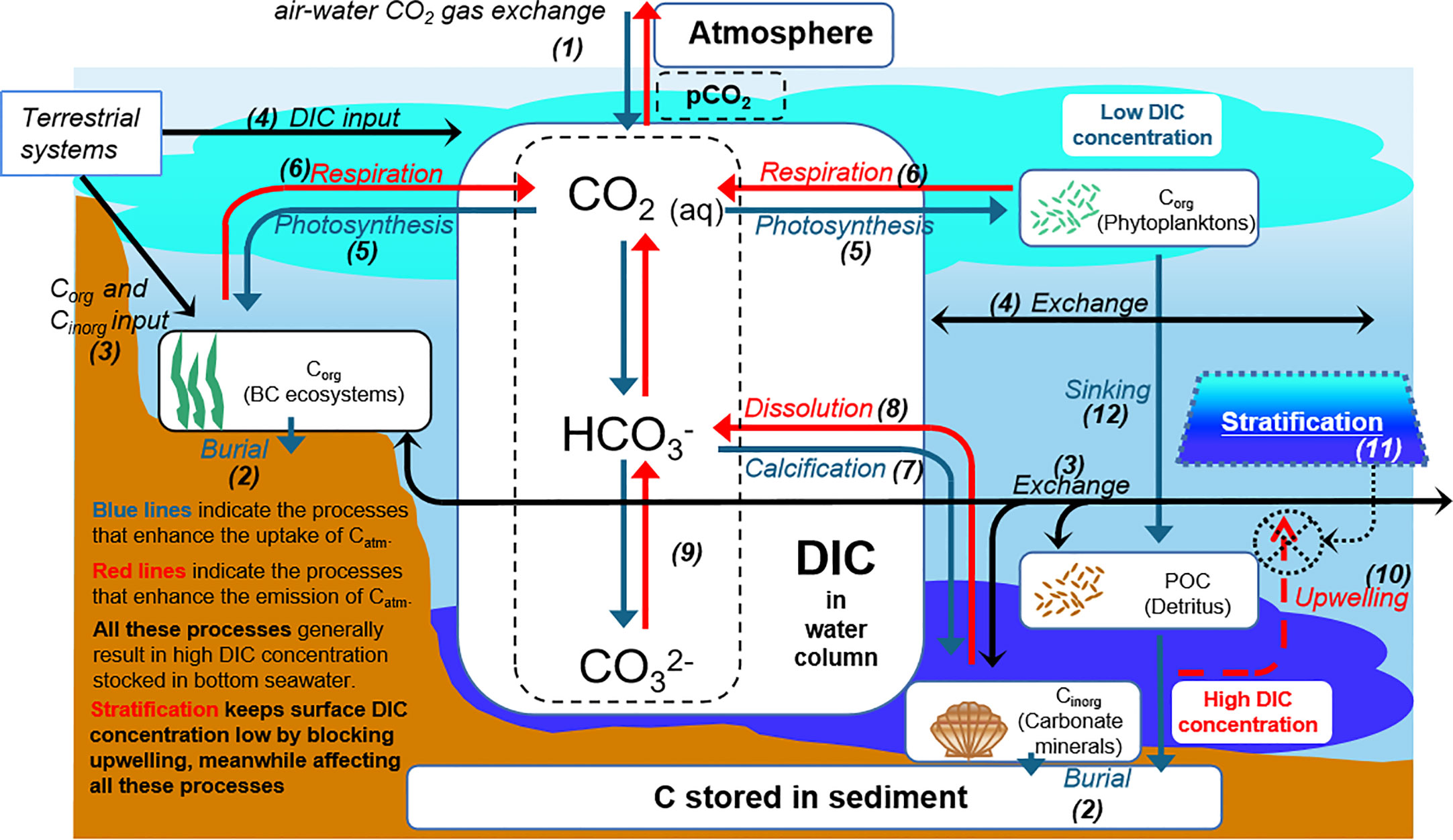
Figure 1 Schematic diagram of CO₂ dynamics in shallow coastal waters.

Here, we discuss the fundamental processes that critically affect the distribution and dynamics of DIC and surface pCO₂ in SCWs. Surface water DIC and pCO₂ would be reduced, since allochthonous organic carbon (C_org) and inorganic (C_inorg) ((3) in Figure 1) and DIC inputs ((4) in Figure 1) are low. Net autotrophic ecosystems (i.e., seagrasses, phytoplankton) would reduce surface DIC and pCO₂, then show a net uptake for atmospheric CO₂ through photosynthesis ((5) in Figure 1) (Maher and Eyre, 2012; Tokoro et al., 2014; Nakayama et al., 2020). Respiration will increase DIC and pCO₂ ((6) in Figure 1). The formation of calcium carbonate minerals will decrease DIC by calcification ((7) in Figure 1) and increase DIC by dissolution ((8) in Figure 1). Additionally, the reactions of the DIC cycle ((9) in Figure 1) can change the pCO₂ in surface water and therefore affect the net exchange of CO₂ with the atmosphere (Howard et al., 2017; Macreadie et al., 2017; Howard et al., 2018). According to these processes, the DIC in bottom water is generally much higher than that in surface water and will usually mix with surface water by upwelling ((10) in Figure 1). However, stratification ((11) in Figure 1) occurs seasonally in SCW regions, mainly in summer (Wakeham et al., 1987; Wiseman et al., 1997), which can hinder the upwelling of bottom water with a high DIC concentration to suppress increases in DIC and pCO₂ in the surface water. In addition, unlike the effects of stratification on bottom DIC behavior, the sinking of particle organic carbon (POC) ((12) in Figure 1) from seawater surface is not hindered by stratification (Koné et al., 2009).

Stratification controls DIC and the vertical distribution of other water properties (i.e., water temperature, salinity, nutrients, phytoplankton, and dissolved oxygen) (Sylaios et al., 2006; Boldrin et al., 2009; Howarth et al., 2011). Water temperature negatively correlates with CO₂ solubility, and DIC in seawater shows a strong dependence on salinity in several shallow coastal regions (Bakker et al., 1999; Eyre, 2000). Phytoplankton in surface water can reduce pCO₂ through photosynthesis, and nutrients enhance the growth of phytoplankton and other net autotrophic ecosystems. Moreover, stratification suppresses the upwelling of suspended particles from bottom waters; improves transparency, thereby promoting photosynthesis; and decreases the amount of pCO₂ in the surface water (Chen et al., 2008). Furthermore, despite the controversy, studies have shown that the mineralization rate is low under hypoxic conditions caused by stratification (Hartnett et al., 1998; Koho et al., 2013). These results indicated that stratification appears to be a critical environmental parameter for the distribution and dynamics of DIC and pCO₂ in SCWs, thereby strongly affecting the F_CO2. Moreover, many studies have reported the potential relationship between CO₂ dynamics and stratification in coastal seawater, but since these studies only measured CO₂ data in surface seawater, the interaction between CO₂ dynamics and stratification in the detailed water column is still unclear (Shim et al., 2007; Zhai and Dai, 2009; Wang and Zhai, 2021). For this purpose, fully understanding the effects of stratification on submerged carbon biogeochemical processes and air–water CO₂ exchanges in SCWs is highly significant for helping us to understand the role of SCWs in climate change mitigation.

Field measurement is generally considered one of the most effective methods for determining the biogeochemical distribution and dynamics of seawater. Recently, researchers have conducted several field measurements to assess the DIC and pCO₂ dynamics in the water column of SCWs in order to estimate their contribution to atmospheric CO₂ removal (Koné et al., 2009; Chen et al., 2013; Kubo et al., 2017). However, these field measurements were conducted in surface seawater on a monthly or annual scale, but the complicated vertical distribution and dynamics of DIC and pCO₂ caused by short-term temporal events (namely, stratification) in the water column, which could be considered to affect the entire carbon absorption and storage cycle, are still unknown. Thus, field measurements conducted under several different stratification conditions are needed in order to clarify the DIC and pCO₂ vertical distribution and dynamics in SCWs. However, in the case of research on the characteristics of water quality dynamics in SCWs focusing on stratification and upwelling, the use of a tiny spatiotemporal scale is necessary, and it is hard to achieve this in field measurements. For this situation, three-dimensional (3D) numerical simulation is an effective measure that complements field measurement data and enables further analyses to be made. One study confirmed the advantages of the application of a 3D numerical model for the reproducibility of DIC and pCO₂ dynamics in the water column of SCWs (Sohma et al., 2018). Still, the model they developed was based on measurement data from surface seawater (Kubo et al., 2017), and the effects of stratification were not considered. Therefore, a 3D numerical model that can accurately describe the DIC and pCO₂ dynamics under the influence of stratification could enable us to better understand the carbon cycle in SCWs and improve the accuracy of F_CO2 estimation.

This study has three primary objectives: (1) to examine the vertical distribution and dynamics of DIC and pCO₂ under different stratified conditions in the Yatsushiro Sea, Japan, by conducting field measurements under the three most representative stratification conditions within the hourly scale; (2) to develop a high vertical resolution hydrodynamic-ecological 3D numerical model that can accurately describe the vertical distribution and dynamics of DIC and pCO₂ under stratified conditions in the bay; (3) to analyze the CO₂ dynamics and the corresponding influence mechanism of the bay and estimate the 2018 F_CO2 through the numerical simulation results.

2 Materials and methods

2.1 Study site and field measurements

The Yatsushiro Sea, which was selected as the target area for this study, is located in the western part of Kyushu Island, Japan (Figure 2). It is a highly enclosed inlet compared to other bays in Japan, and is characterized by a large tidal range and vast tidal flats and brackish water areas. Therefore, a unique ecosystem has developed in the bay’s shallow waters, with high biodiversity and rich biological productivity. The northern part of the bay has a solid inner bay character and tidal flats, while the southern part of the bay, south of the central part, has a rapid seawater exchange and a reef-like seafloor that gradually becomes more pelagic. The southern part of the Yatsushiro Sea and the sea area around the Amakusa Islands have been selected by the Ministry of the Environment as “a sea area of high importance from the viewpoint of biodiversity.” The bay is located along the coast of Kumamoto Prefecture, where the Tsushima Warm Current, a branch of the Kuroshio Current, flows. In particular, the southwestern part of the Amakusa Islands surrounding the bay is a significant habitat for reef-building corals in western Kyushu. The fifth nature conservation survey conducted by the Ministry of the Environment confirmed the existence of seagrass beds covering an area of about 1,141 ha.

FIGURE 2

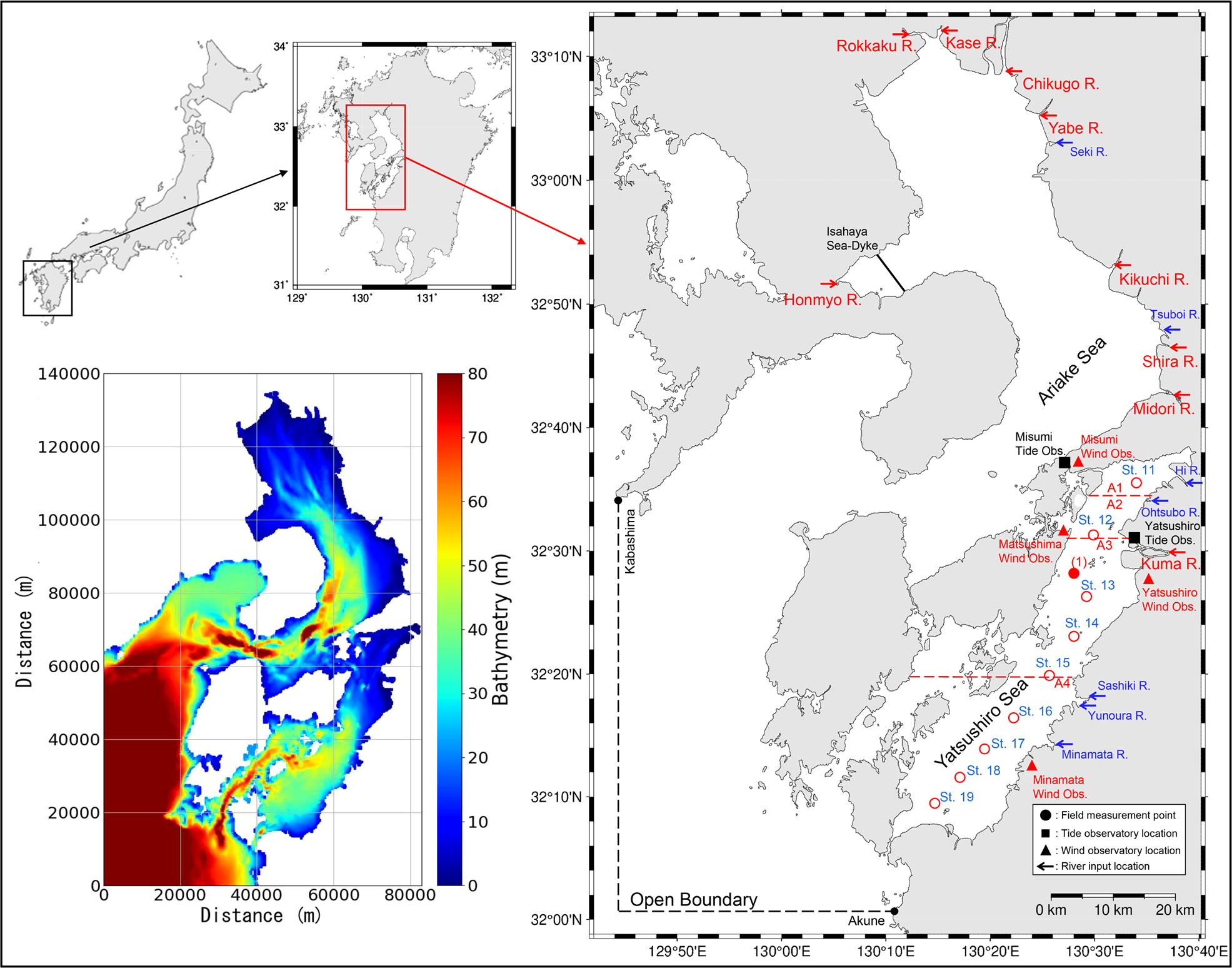
Figure 2 The location of the study site (right) and the domain of the numerical model (bottom left). The field measurement points are shown in the map on the right ((1) is the location of the field measurement we conducted, while St.11 to St.19 are the measurement locations of the data from MLIT), schematic diagram of the Yatsushiro Sea subdivision (A1 to A4 separated by red lines) and the location of the wind observatories (red dots).

The area of the bay is about 1,200 km². The basin area of the rivers flowing into the bay is approximately 3,000 km². Forty-seven rivers (one first-class river, forty-six second-class rivers) flow into the Yatsushiro Sea with a total watershed area of 3400 km², of which one first-class river, the Kuma River, has a catchment area that makes up about 60% of the total. The inflow of fresh water during the rainy season from June to August lowers the salinity throughout the sea area. In the inner part of the bay, the salinity decreases significantly due to the increased inflow of rivers such as the Kuma River.

The Yatsushiro Sea is considered to be a unique coastal area in terms of physical conditions such as flow, topography, and ecosystem. Since there is a lack of knowledge about blue carbon ecosystems (i.e., phytoplankton, seagrasses such as eelgrass, and corals) inhabiting the bay at the same time, new research results on air-sea CO₂ flux, pCO₂ in seawater, and related environmental factors in the bay are expected.

We conducted field measurements of the CO₂ dynamics in seawater at point (a) (32°27′30” N, 130°27′37” E, mean water depth: 20 m), which was the first attempt to investigate the seawater CO₂ dynamics in the Yatsushiro Sea. The measurement point is relatively close to the estuary of the Kuma River, where strong salt stratification is expected during flooding. The three measurement dates were all during spring tides and showed weak stratification (26 August 2018), mixed conditions (7 December 2018), and strong stratification (2 August 2019). CTD measurements and water sampling were conducted during a half-tide period (approximately 6 h) from high tide (9:00 am) to low tide (3:00 pm). CTD measurements included vertical profiles of the water temperature, salinity, and water density. Water samples were used for the analysis of DIC and TA. CTD measurements were conducted approximately every 20 min using a multi-item water quality meter (ProDSS, YSI). Water samples were collected at high tide, 1.5 h after high tide, at the full ebbing tide, 1.5 h before low tide, and at low tide, with 30 samples collected for each measurement. The samples were collected in 250 mL Duran bottles, and the DIC and TA were fixed by injecting mercury dichloride solution (250 mL). The values of DIC and TA were analyzed using a flow-through carbonate analyzer (MDO-02, made by Kimoto Electronics Co., Ltd.) and a total alkalinity titrator (ATT-15, made by Kimoto Electronics Co., Ltd., Osaka, Japan) owned by Kitami Institute of Technology. From the obtained DIC, TA, salinity, and water temperature, pCO₂ was calculated from the semi-empirical equations for carbon-based chemical equilibrium (Zeebe and Wolf-Gladrow, 2001). The equation used in this study was the one developed in the ‘seacarb’ package in the R software (Lavigne and Gattuso, 2010).

The results of these three measurements were used for the calibration and validation of model values near the estuary of the Kuma River. In addition, St.11 to St.19 are the locations of the regular sites used for the environmental measurement of the water quality of the Yatsushiro Sea by the Ministry of Land, Infrastructure, Transport, and Tourism (MLIT) of Japan (Figure 2). The measurements included the vertical distribution of the water temperature, salinity, and seawater density at each site. In principle, the measurement frequency was twice a month (canceled in exceptional cases). The measurement results were used to calibrate and validate the simulation results of the CTD profiles in the whole area of the bay in this study.

2.2 Description of numerical model

Delft3D is an open-source 2D/3D numerical simulation software package that was developed by WL Delft Hydraulics (currently known as Dertares) (Lesser et al., 2004; Deltares, 2017). The software is a flexible framework for simulating water flow; water quality; waves; ecology; sediment transport in fluvial, estuarine, and coastal environments; and the interactions between the various processes.

In this study, the FLOW and WAQ modules in Delft3D (version 4.04.01) were utilized as the modeling tools. This framework has been effectively implemented to simulate ocean circulation, stratification, and water quality in various coastal waters (Niu et al., 2016; Alosairi and Alsulaiman, 2019). There have been several successful cases where the CO₂ cycle was simulated in surface water by applying the Delft3D-WAQ module (Menshutkin et al., 2014; Chen et al., 2019).

2.2.1 Hydrodynamic model Delft3D-FLOW

The mathematical principle of the hydrodynamic model Delft3D-FLOW is mainly to solve the Reynolds-Averaged Navier–Stokes (RANS) equations for incompressible fluids under shallow water assumptions using the finite difference method.

In this study, we refined the resolution of the vertical direction to further improve the accuracy of the vertical direction based on a general 3D coastal current model developed by Yano et al. (Yano et al., 2010) in order to simulate the effects of stratification more accurately. The computational domain of this model, which covers both the Ariake Sea and the Yatsushiro Sea (Figure 2).

A Cartesian coordinate system with a resolution of 10” (Δx = 250 m) was used in the horizontal direction, while a σ-coordinate system with 17 layers (2% × 10 layers, 5% × 1 layer, 10% × 3 layers, and 15% × 3 layers from the surface to the bottom, respectively) was used in the vertical direction. Horizontal eddy viscosity and eddy diffusion coefficients were evaluated using the Subgrid scale (SGS) model, and vertical eddy viscosity and eddy diffusion coefficients were evaluated using the k-ϵ turbulent model and incorporated into the tidal flatness model (dry-wet model). The calculation time frame was from 1 January 2018 to 1 January 2019, with a time step of 3 min.

The open boundary was located on the line connecting Akune, Kagoshima Prefecture, and Kabashima Strait, Nagasaki Prefecture (Figure 2). The known harmonic constants at both ends of the open boundary are estimated from measured data from 1970 and 1891 for Akune and Kabashima Suido, respectively, and the amplitudes and phase lags of major four tide components (M2, S2, K1, and O1) were adjusted according to the existing harmonic constants at both ends by Yano et al. (Yano et al., 2010). The setting of harmonic constants using in this model were shown in Table 1. A constant value of 35.15 psu was used for the salinity in the open boundary condition, with the water temperature of sea surface and seabed were using a time series obtained from the daily sea surface temperature data and data at a depth of 50 m from the Fukuoka Regional Meteorological Observatory.

TABLE 1

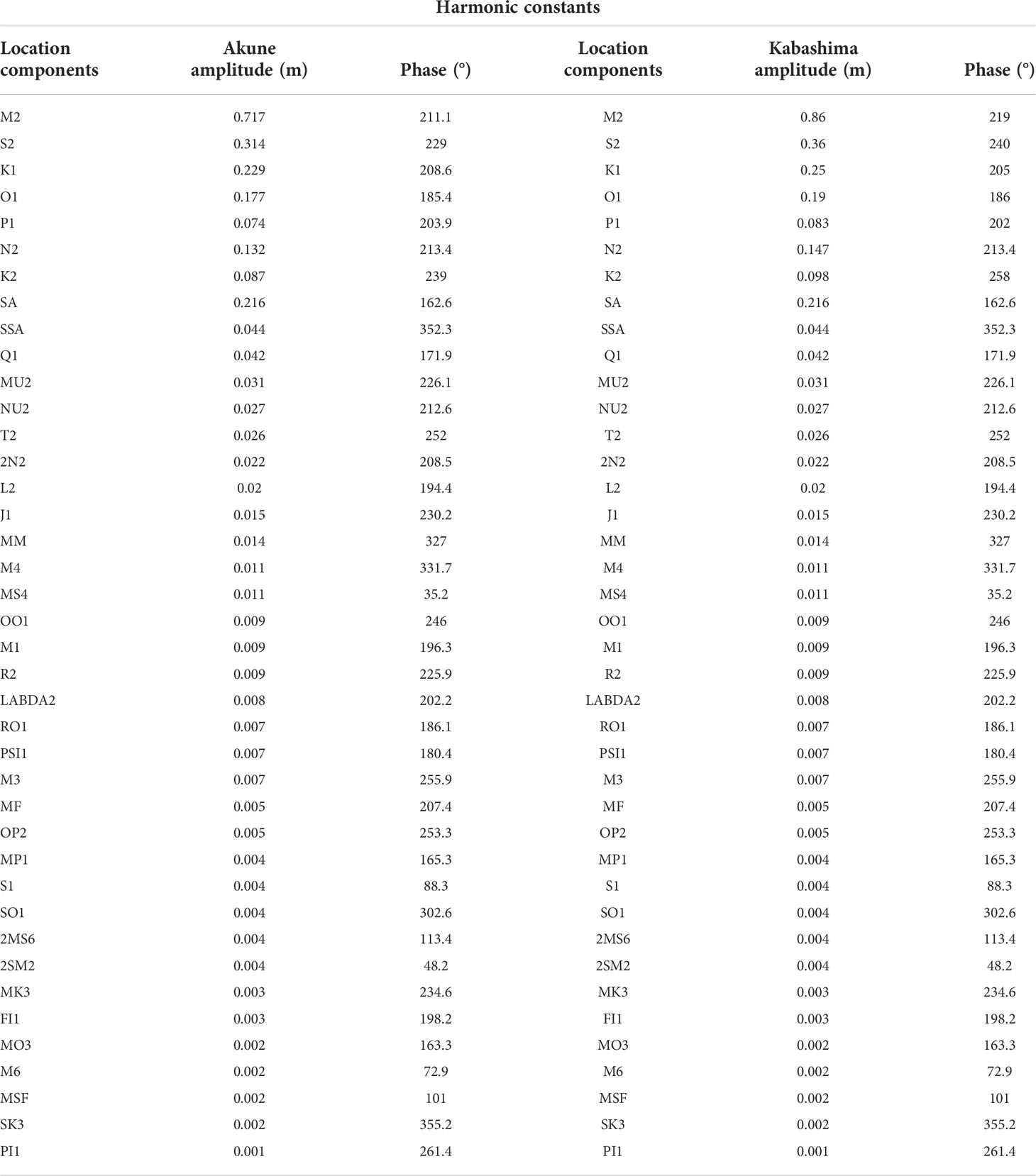
Table 1 Harmonic constants of hydrodynamic model.

In this study, freshwater inflows from eight first-class rivers (Chikugo, Yabe, Kase, Rokkaku, Kikuchi, Shira, Midori, and Kuma) and nine major second-class rivers (Kashima, Shioda, Seki, Tsuboi, Hi, Otsubo, Sashiki, Yunoura, and Minamata) were considered (Figure 2). The flow rate of the first-class rivers was the hourly flow rate at the station nearest to the estuary in the non-tidal area obtained from the hydrological water quality database of the MLIT. To account for the inflow downstream of the station, the flow rate at the station was corrected by multiplying it by a factor calculated by dividing the station’s catchment area by the total area of the watershed. For second-class rivers, the calculation was based on the ratio of the catchment area to nearby first-class rivers.

The solar radiation, air temperature, humidity and wind data used in this model were a hourly time series, and were obtained from Kumamoto station and Yatsushiro station of Japan Meteorological Agency (JMA) Amedas, respectively. The wind speed was converted to equivalent sea breeze using Carruthers’ land boundary wind to sea breeze conversion coefficient (Arakawa et al., 2007).

In this model, we used the region-wide average salinity and water temperature of the calculated area as of December 31, 2017, obtained from the same model calculation in the previous year, i.e., 2017, as the initial constant conditions. Model calculations for both the hydrodynamic and ecological models used a cold start from January 1, 2018, with a stabilization period of approximately 2 weeks, which did not affect the model validation results since our calibration and validation of the models started in mid-January, but had a small effect on the CO₂ flux calculations in January.

2.2.2 Ecological model Delft3D-WAQ

Delft3D-WAQ is a module of the ecological section that is used to simulate biological processes in water bodies and sediments and various processes of solute transport and transformation. The WAQ module mainly solves the advection–diffusion–reaction equations for each computational grid by combining the results of the FLOW module (e.g., the spatial and temporal distribution of salinity, water temperature, velocity, and turbulence dispersion coefficient). Therefore, the computational domain, resolution, number of layers in the σ-coordinate system, location of the freshwater inflow, and flow velocity are the same as those in the hydrodynamic model. In addition, all the physical conditions used for the FLOW module (e.g., the solar radiation, air temperature, humidity, wind, river inflow) were coupled into the WAQ module, and the start pattern (e.g calculation time frame and time step) were the same as the FLOW module. This ecological module offers the user a wide range of frameworks for choosing the substances and processes to be simulated, giving more flexibility in simulating physical, biochemical, and biological processes (Deltares, 2018). The structural diagram of the ecological model used in this study (Figure 3). The interaction of phytoplankton dynamics, nutrients cycling, and inorganic carbon cycling are considered in this model as the key process affecting the objective of this study (i.e., pCO₂ dynamics in the water column).

FIGURE 3

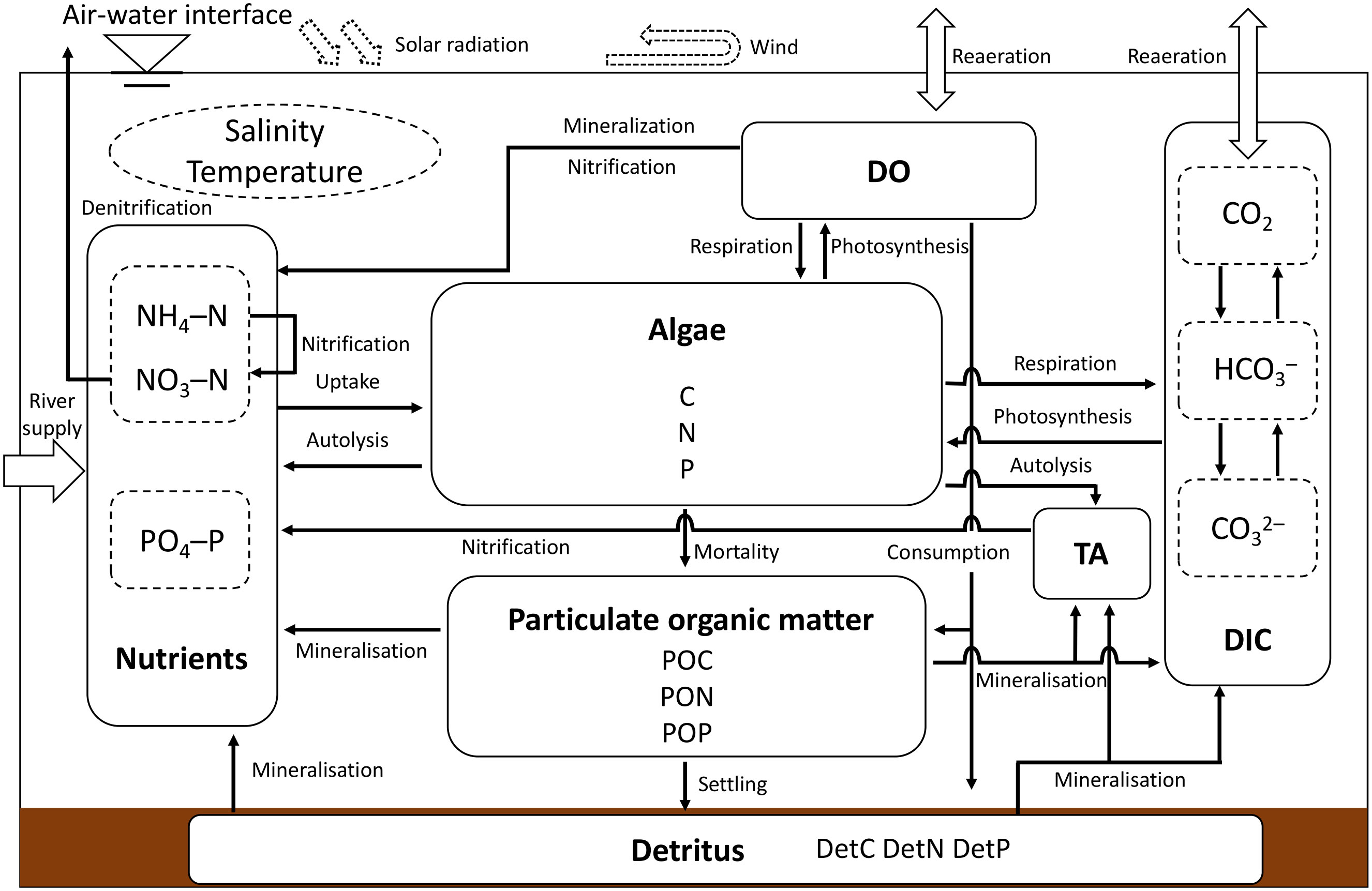
Figure 3 Structural diagram of the ecological model (modified from the generic ecological model developed by Blauw et al. (Blauw et al., 2008)).

The model settings of this ecological model were chosen mainly by referring to the settings of the generic ecological model (GEM) (Blauw et al., 2008), and the detailed model setup parameters are shown in Table 2. Considering the wide coverage of this model and the complex physical and biochemical processes in the target waters, we simplified the GEM by considering only one phytoplankton species (i.e., green algae) and assuming the decomposition rate of dissolved organic matter to be that of the inorganic matter immediately after production. This simplification has been proven to be reliable in previous simulation studies for anoxic states in the Ariake Sea (Tadokoro and Yano, 2019; Hao et al., 2021). Based on the simplified model, we added the processes of DIC, TA, and pH to simulate the CO₂ dynamics in the water column.

TABLE 2

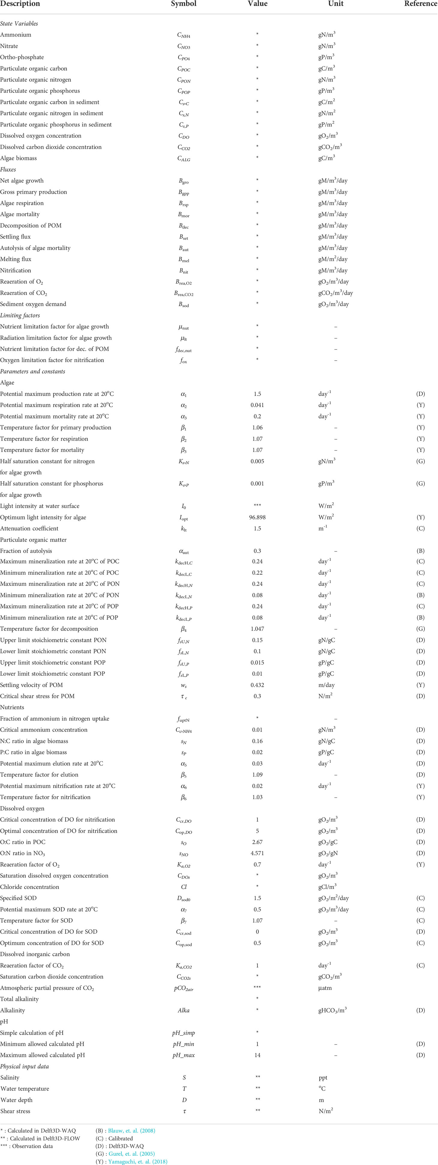
Table 2 Process parameters of the ecological model.

There are three main processes that are related to phytoplankton in Delft3D-WAQ: gross primary production, respiration, and mortality. Gross primary production is the total amount of energy produced through the process of photosynthesis. By capturing the energy from sunlight, primary producers can store it in organic compounds by converting carbon dioxide and water into organic compounds (Falkowski and Raven, 2013). In this model, three factors are chosen to affect the rate of gross primary production, temperature, availability of nutrients, and light. A higher temperature increases the rate of the chemical processes taking place within the algal cells. Thus, lowering the temperature limits the growth of algal biomass (Deltares, 2018). Phytoplankton require chemical elements to function, and the most vital aspects are nitrogen and phosphorus. The limitation factor is calculated according to the Monod equation for each nutrient, where the lowest value amongst these is used. The limitation of nitrogen is chosen to be dependent on the sum of the total concentration of ammonium and nitrate. The third factor, light, is necessary in order for the process of photosynthesis to take place. The extinction of light depends on the water depth and the concentration of absorbing substances within the water, which here are determined to be algal biomass, particulate organic matter (POM), humidity input from freshwater, and background absorption. The extinction of light is calculated according to Lambert–Beer’s law, where the light intensity is reduced exponentially along with the water depth in relation to the intensity at the surface. Dissolved inorganic carbon (DIC) is also regarded as a rate-limiting resource for phytoplankton, as indicated by the availability of CO₂ and bicarbonate (HCO₃) for photosynthesis (Verspagen et al., 2014). In this model, respiration is performed when the algal cell grows (increasing biomass) and to maintain the functions of the cell—i.e., the basal metabolism. The respiration rate necessary to keep the cell alive is related to the temperature. The mortality rate of algae is a function of temperature, where a higher temperature promotes a higher mortality rate. When algae die, a fraction of their biomass is directly released to the water as already dissolved inorganic matter. This process is called autolysis. However, the majority of the biomass stays intact and continues in the nutrient cycle as detritus, here referred to particulate organic matter.

This model simulates the simplified cycling of two types of nutrients: nitrogen and phosphorus. It includes three significant pools within the nutrient cycle: dissolved inorganic nutrients (NH4-N, NO3-N, and PO4-P), living organic matter (Algae), and POM. The uptake of nutrients is an equivalent result of the growth of algae. Hence, the consumed nutrient flux is proportional to the net primary production obtained using the N:C and P:C ratio in the algal biomass. Following the death of algae, the nutrients are either released back into the water body in the form of dissolved inorganic nutrients through autolysis or released back as detritus or dead organic matter. The release of nutrients by dead algae is equivalent to the N:C and P:C ratios within the algal biomass. Carbon, nitrogen, and phosphorus in the detritus are simulated as the state variables of particulate organic carbon (POC), particulate organic nitrogen (PON), and particulate organic (POP). POM comes from discharging rivers or the mortality flux of dead algae. The latter occurs through the process of mineralization, where microorganisms decompose POM into inorganic components. When algae and higher plants die, detritus is produced. Mineralization is the microbial decomposition of detritus into its fundamental inorganic components, such as carbon dioxide, ammonium, and phosphate. POM settles into the sediment during the settling process. In this case, the settling velocity is constant throughout time and unaffected by the bottom shear stress. Different forms of POM are subjected to the same settling velocity.

The main processes of inorganic carbon balance are air–water CO₂ exchange, the mineralization of organic carbon to inorganic carbon, and primary algal production. The reaeration of carbon dioxide proceeds proportionally to the difference between the saturated CO₂ concentration and the actual dissolved CO₂ concentration. The reaeration quantity per day was equivalent to the F_CO2 diffused across the air-water interface. CO₂ in surface water tends to be saturated relative to the atmospheric CO₂ concentration. However, CO₂ production and consumption processes in the water column counteract the saturation, resulting in either a CO₂ excess or a CO₂ deficit. The saturation concentration of CO₂ in the water column is primarily a function of the atmospheric pCO₂, the water temperature, and the salinity. However, the pCO₂ in the atmosphere is assumed to be constant. In Delft3D-WAQ, the calculation of the saturation concentration is performed as a separate process, which has been implemented with two alternative formulas (Weiss, 1974; Golterman, 1982). In this study, we applied Weiss’ formula. The pH, the carbonate speciation (CO₂, pCO₂, H₂CO₃, HCO₃⁻, and CO₃²⁻), and the saturation states of calcium carbonate (calcite and aragonite) in the water column and the sediment bed could be calculated from the TA and the DIC according to the carbon chemical equilibrium. Salinity and temperature from the hydrodynamic model are necessary inputs.

2.3 Model calibration and validation

In this study, the calibration and validation of the model were carried out in two steps. The first step involved calibrating and validating the hydrodynamic and ecological model parameters for the easily stratified area near the Kuma River estuary using the results of three field measurements of CO₂ dynamics in seawater at different stratification periods implemented at point (a) in Figure 2. The second step involved calibrating and validating the simulation results of the horizontal and vertical distribution of CTD for the whole area of the Yatsushiro Sea for the whole year of 2018 using CTD measurement data from the central route of the bay (the line from St.11 to St.19 in Figure 2) from the MLIT. In the first validation step, we performed a comparative validation of the water temperature, salinity, density, DIC, TA, and pCO₂, containing statistical analysis and contour plot comparison. In the second step, we calibrated and validated the water temperature, salinity, and seawater density. In addition, we applied the concept of density stratification index (SI) proposed in (Simpson et al., 1990) for quantifying the strength of density stratification. Based on the process of calibrating and validating the SI, we improved the simulation accuracy of the hydrodynamic model for the stratification state of the whole area of the bay. The equation for calculating the SI is shown in Equation (1) (Simpson et al., 1990):

$\begin{array}{ll}SI=-\frac{1}{H}\underset{-H}{\overset{0}{\int }}\left(\rho -\overline{\rho }\right)g·z·dz& (1)\end{array}$

where ρ = ρ (z) is the water density profile over the water column of depth H, bar is depth averaging, g is the gravitational acceleration, and z is the vertical coordinate.

To quantitatively evaluate the model performance, three performance metrics were selected: the root mean square error (RMSE), the Pearson’s correlation coefficient ^®, and the refined Willmott index (d_ref). A “good” model has a low RMSE. The Pearson’s correlation coefficient r was used to evaluate the model performance. A value of 1 shows a good correlation between measurements and simulation, whereas values near 0 suggest weaker and often inconsequential correlations. The refined Willmott index d_ref is a modeling efficiency index that ranges from −1 to 1. A value that is closer to 1 suggests that the model is performing better. The equation for calculating the d_ref is shown in Equation (2) (Willmott et al., 2012). To verify the model’s reproducible performance of the CTD distribution and CO₂ dynamics in seawater in the vertical direction, we also used contour plots to compare the simulation results with measurements.

$\begin{array}{ll}{d}_{ref}=\{\begin{array}{l}1-\frac{{\displaystyle {\sum }_{i=1}^n\left|m_i-o_i\right|}}{2·{\displaystyle {\sum }_{i=1}^n\left|o_i-\overline{o}\right|}},\text{when}\\ {\displaystyle {\sum }_{i=1}^n\left|m_i-o_i\right|}\le 2·{\displaystyle {\sum }_{i=1}^n\left|o_i-\overline{o}\right|}\\ \frac{2·{\displaystyle {\sum }_{i=1}^n\left|o_i-\overline{o}\right|}}{{\displaystyle {\sum }_{i=1}^n\left|m_i-o_i\right|}}-1,\text{when}\\ {\displaystyle {\sum }_{i=1}^n\left|m_i-o_i\right|}>2·{\displaystyle {\sum }_{i=1}^n\left|o_i-\overline{o}\right|}\end{array}& (2)\end{array}$

where m_i: simulated values, o_i: measured values, $\overline{m}$ : mean of simulated values, $\overline{o}$ : mean of measured values, n: the number of measurement data.

2.4 Model-based simulation of CO₂ dynamics in SCWs

We applied the developed hydrodynamic-ecological model to simulate the CO₂ dynamics in the whole area of the Yatsushiro Sea for the entire year of 2018. Based on the simulation results, we analyzed the dynamics of CO₂ in the bay in horizontal and vertical directions at different periods and the corresponding influence mechanism. In addition, we also analyzed the changes in the CO₂ dynamics in seawater during the flooding period, which is the period where there are large fluctuations in stratification conditions, and the corresponding influence mechanism by comparing the vertical dynamics of the areas in the Yatsushiro Sea that are more and less influenced by freshwater inflow during the flooding period.

Finally, we used the model to estimate the F_CO2 between seawater and the atmosphere in the Yatsushiro Sea during the full year of 2018. The F_CO2 was calculated using the block volume method shown in Equation (2) with the pCO₂ in seawater, atmospheric pCO₂ (pCO_2air), the solubility K₀, and the exchange coefficient k. pCO_2air was set based on observation data from the JMA (at Ayari). It was indicated that the atmospheric CO₂ concentration (ppm) was numerically almost equal to the pCO₂ in the atmosphere (µatm). Therefore, the annual average measured value of 412 ppm for 2018 was converted to 412 µatm and assumed to be constant throughout the year.

$\begin{array}{ll}{F}_{CO2}=k·K_0·(pC{O}_2-pC{O}_{2air})& (3)\end{array}$

When the F_CO2 is negative, it represents absorption from the atmosphere to seawater, while when it is positive it represents emission from seawater to the atmosphere. The solubility K₀ (mol/m³/atm) was determined from the empirical equation based on the water temperature and salinity (Weiss, 1974). The exchange coefficient k was obtained from Equation (4) (Wanninkhof, 1992).

$\begin{array}{ll}k=0.39·U_{10}{2}^{·}{(\frac{S_c}{660})}^{-0.5}& (4)\end{array}$

where U₁₀ is the wind speed (m/s) at a height 10 m above the sea surface, S_c is the Schmidt number of CO₂, and S_c is derived from the empirical equation (Wanninkhof, 1992).

Due to the large area of the Yatsushiro Sea, it was difficult to obtain very accurate wind speed data for the calculation of F_CO2. Figure 2 shows the wind observation stations around the bay. In order to estimate F_CO2 more precisely, we divided the bay into four areas (see A1 to A4 in Figure 2) near four wind observation stations by referring to the results of water quality and environmental characteristics analysis of the bay (Sonoda et al., 2013), then calculated the F_CO2 using wind data obtained from Misumi Wind Obs., Matsushima Wind Obs., Yatsushiro Wind Obs., Minamata Wind Obs. (Figure 2) for areas A1, A2, A3, A4 separately.Also, the wind speed data was converted to equivalent sea breeze using the same method in Section 2.2.1.

In addition, U₁₀ was corrected in height by a power law from the data of each observatory shown in Equation 5 (Ishizaki and Mitsuta, 1962).

$\begin{array}{ll}{U}_{10}=U_Z·{(\frac{10}{Z})}^{\frac{1}{n}}& (5)\end{array}$

where U_Z is the wind speed (m/s) at altitude Z (m) and n is a constant determined by the surface conditions at the observation site.

3 Results and discussion

3.1 Field measurement results and model calibration and validation near the estuary

The results of the three field measurements we implemented at point (1) were used for the calibration and validation of the numerical model simulation results near the estuary of the Kuma River. The final statistical validation results are displayed in Table S1. Among these, salinity, σ_t, and water temperature were used for the verification of the hydrodynamic module. There was a strong correlation between the simulated CTD results and the measured values (r > 0.9). The highest correlation was found for water temperature (r > 0.97), but its RMSE was relatively high, probably since the measurement site was located near the estuary of the Kuma River and was thus strongly influenced by the freshwater inflow. The river temperature data input to the model was obtained from the prediction of the L–Q equation based on the temperature and flow of the previous years, which contained some errors. The RMSE of both σ_t and salinity showed low values (0.95 kg/m³ and 0.92 psu). The d_ref values for each variable indicated that the model had a good performance (>0.6) for the hydrodynamic simulation of this region. In general, the model’s hydrodynamic simulation performance in the Kuma River estuary was in an acceptable range overall, where the performance of the variation trend was better than the numerical fitting performance. Otherwise, since we changed the grid and increased number of layers of the hydrodynamic model developed by Yano et al., we validated the tidal level results at two sites (Misumi Tide Obs. and Yatsushiro Tide Obs. in Figure 2), which showed a good fit, as shown in Figure S2.

The biogeochemical variables (DIC, TA, and pCO₂) were chosen for the verification of the ecological model. Regarding the value of DIC, it had a Pearson correlation value of 0.94, showing a very strong correlation, while the RMSE of 33.10 μmol/kg was at a low level (1.74%) relative to the mean of the measured DIC (1899.4 μmol/kg). The simulated TA also showed a very strong correlation for the measured data (r = 0.94), and the ratio of RMSE to the mean of the measured values was at a very low level (2.16%). While the value of r of pCO₂ was lower (0.87) relative to the last two, but again showed a strong correlation, its RMSE value (65.56 μatm) was slightly higher (15%) relative to the ratio of the mean of the measured values, but still in an acceptable range (<30%). The reason for the large numerical errors in pCO₂ while DIC and TA had good numerical fits was that pCO₂ was calculated based on water temperature, salinity, DIC, and TA, and small errors in each of these were superimposed on the final pCO₂ calculation, resulting in large errors in pCO₂; this is a major challenge for pCO₂ simulation in water bodies. Overall, the ecological model had a relatively good performance in simulating the CO₂ dynamics in the Kuma River estuary region, as shown by the d_ref values (>0.6) of DIC, TA, and pCO₂.

In addition, we visualized the contour plots of the measured and simulated results separately. The variables output from the hydrodynamic model (i.e., salinity, σ_t, and water temperature) are shown in Figure S2, while the output of the variables from the ecological model (i.e., DIC, TA, and pCO₂) is shown in Figure S3.

Based on the vertical distribution of σ_t (Figure S2A), we confirmed that the field measurements were in the mixing period (7 December 2018), the weakly stratified period (26 August 2018), and the strongly stratified period (2 August 2019). In addition, the vertical distribution of salinity and water temperature show that the region also produces thermohaline stratification similar to the density stratification. As for the results of contour plots of DIC, TA, and pCO₂ (Figures S3A, C, E), the CO₂ dynamics in the water column shows a similar distribution state to that of density stratification.

The comparison of the simulated and observed values of σ_t shows that there were good fitting results for all periods (Figures S2A, B). The maximum error was only about 1 psu. And it had an excellent fitting performance for the periods in strong stratification. The bottom layer was basically consistent at 22 psu, and the error in the surface layer was about 1 psu. The other variables also showed a more excellent fit performance. However, in the simulation of pCO₂ during weak and strong stratification (Figure S3F), the state of high pCO₂ in the bottom layer under stratification was not well simulated. One of the more important reasons for this may be that the ecological module of the model did not consider the influence of zooplankton and benthic organisms, such as the process of their respiration, causing the increase in CO₂ concentration in the bottom water column not to be represented. These advanced biological processes could be added gradually in subsequent modeling. Although the simulation results of pCO₂ in the bottom layer were not satisfactory, the surface pCO₂, which mainly controls the air–water CO₂ exchange, showed a better fitting performance. Moreover, the overall CO₂ dynamic stratification state was better simulated. In summary, the simulated performance of the ecological module for CO₂ dynamics in the Kuma River estuary region was acceptable for our further analysis of the CO₂ dynamics in stratified SCWs.

3.2 Model validation of the whole Yatsushiro sea

Based on the good model fit results near the estuary of the Kuma River ((1) in Figure 2), we adjusted the hydrodynamic conditions of the hydrodynamic module to optimize the applicability of the model regarding the hydrodynamic simulation of the whole area of the Yatsushiro Sea. The process was based on regular twice-monthly measurements of the bay central route (i.e., the line of nine measurement sites between St.11 and St.19 in Figure 2) implemented by the MLIT in 2018 to calibrate and validate the simulation results. The verified variables were salinity, σ_t, and water temperature. The validation results of the surface and bottom layers of the CTD results for each site are shown in Figure S4. As in Section 3.1, we calculated the r, RMSE, and d_ref values between the simulated and measured values for each site; the results are presented in Table S2.

Then, we checked the output of the contour plot, where the x-axis represents the distance between each measurement sites (St.11 to St.19 shown at the top of each figure). We selected the more representative ones among the many comparison results—that is, the results of three time points similar to the mixing period, weak stratification period, and strong stratification period in 3.1—to show. The results are shown in Figure S5.

In addition, we calculated the stratification index of field measurements and model calculations for each station separately according to Equation 1 and made a comparison plot between the simulated and measured values shown in Figure S6.

We also calculated r, RMSE, and d_ref for the comparison results of each station (Figure S6). The results show that the model performance for each site was within an acceptable range (Most of the r values were greater than 0.6, except for the salinity of St. 11 and St. 12). St.16, St.17, St.18, and St.19, which are farther from the Kuma River estuary and located in the southern part of the bay, showed excellent relations (r > 0.9). In contrast, St.13, St14, and St.15, which are located northward near the estuary of the Kuma River, performed relatively poorly. This is due to the fact that simulating areas with a large freshwater inflow, which is one of our main objectives in this study, is indeed a huge challenge. However, in general our results were still in an acceptable range (r > 0.6). In contrast, the fit performance of St.11 and St.12, located in the northernmost part of the bay, was poorer (r< 0.3), probably because the strength of the model lay in simulating the stratification phenomenon of seawater. The water depth in this region, being too small, makes it easy to produce results that exceed expectations.

3.3 Discussion of model calibration and validation

As for the calibration and validation of this model, our study was the first attempt to investigate the seawater CO₂ dynamics in the Yatsushiro Sea, which has not been studied before, and these three samples were the only actual measurements of seawater CO₂ in the Yatsushiro Sea, and our planned larger-scale field measurements were not successfully implemented due to some force majeure factors. Although we have only three carbonate measurements from one site, these three measurements are different from the conventional time scale of seawater carbonate measurements, which are often measured in days and sampled only on the surface of the seawater, but are precise measurements in the vertical direction in the water column over half a tidal period with a time interval of 1.5 hour. The three measurement periods were chosen to represent the different mixing states of the shallow seawater to a large extent, including the strongly stratified, weakly stratified and mixed periods, and to cover the seasonal factors.

Based on the validation of these three measurements, we were able to determine that the developed coupled hydrodynamic-ecological model has a relatively good performance in the Kuma River estuary area. In the subsequent analysis, we would like to extend the model to apply to the entire Yatsushiro Sea, although we were unable to calibrate and validate the CO₂ in other areas of the Yatsushiro Sea due to the constraints of the lack of measured data. For this situation, we calibrated and validated the CTD field measurements at nine stations spanning the north and south of the Yatsushiro Sea in the vertical direction throughout the year, and we also quantified the stratification intensity and validated the simulated versus measured values for the stratification intensity as well. Through such a more rigorous, model calibration validation for the biogeochemical and mixing state of the whole area of the Yatsushiro Sea, we verified that the hydrodynamic module of the coupled model can accurately describe the biogeochemical and mixing states in the Yatsushiro Sea in 2018. Moreover, due to the ecological model we developed was based on the coupled hydrodynamic model output, and the parameters of the ecological model were calibrated and validated with three representative biogeochemical and mixed-state measurements in the Yatsushiro Sea. With this model development approach, it is reasonable to assume that combining the ecological model, which can accurately describe the CO₂ dynamics in different mixing states in the Kuma River estuary, with the hydrodynamic model, which can accurately describe the biogeochemical and mixing states in the whole Yatsushiro Sea in 2018, can simulate the CO₂ dynamics in the whole Yatsushiro Sea in an acceptable range, supporting our preliminary analysis of the horizontal and vertical CO₂ dynamics of the entire bay.

However, the calibration and validation method of this model was still weak for simulating the CO₂ dynamics in a highly heterogeneous shallow coastal water. In the future work, more extensive measured data on the CO₂ dynamics of the Yatsushiro Sea with a large temporal and spatial scale are needed in order to improve the simulation performance of the model on the CO₂ dynamics of the entire bay.

3.4 Simulation and analysis of CO2 dynamics in the Yatsushiro sea

We applied the verified model to simulate the CO₂ dynamics of the Yatsushiro Sea for the whole year of 2018. The full-year 2018 Kuma River flow rate and the average density stratification index of the bay are shown in Figure 4A. We can see that the most critical driver of density stratification in the bay is the freshwater inflow from the Kuma River.

FIGURE 4

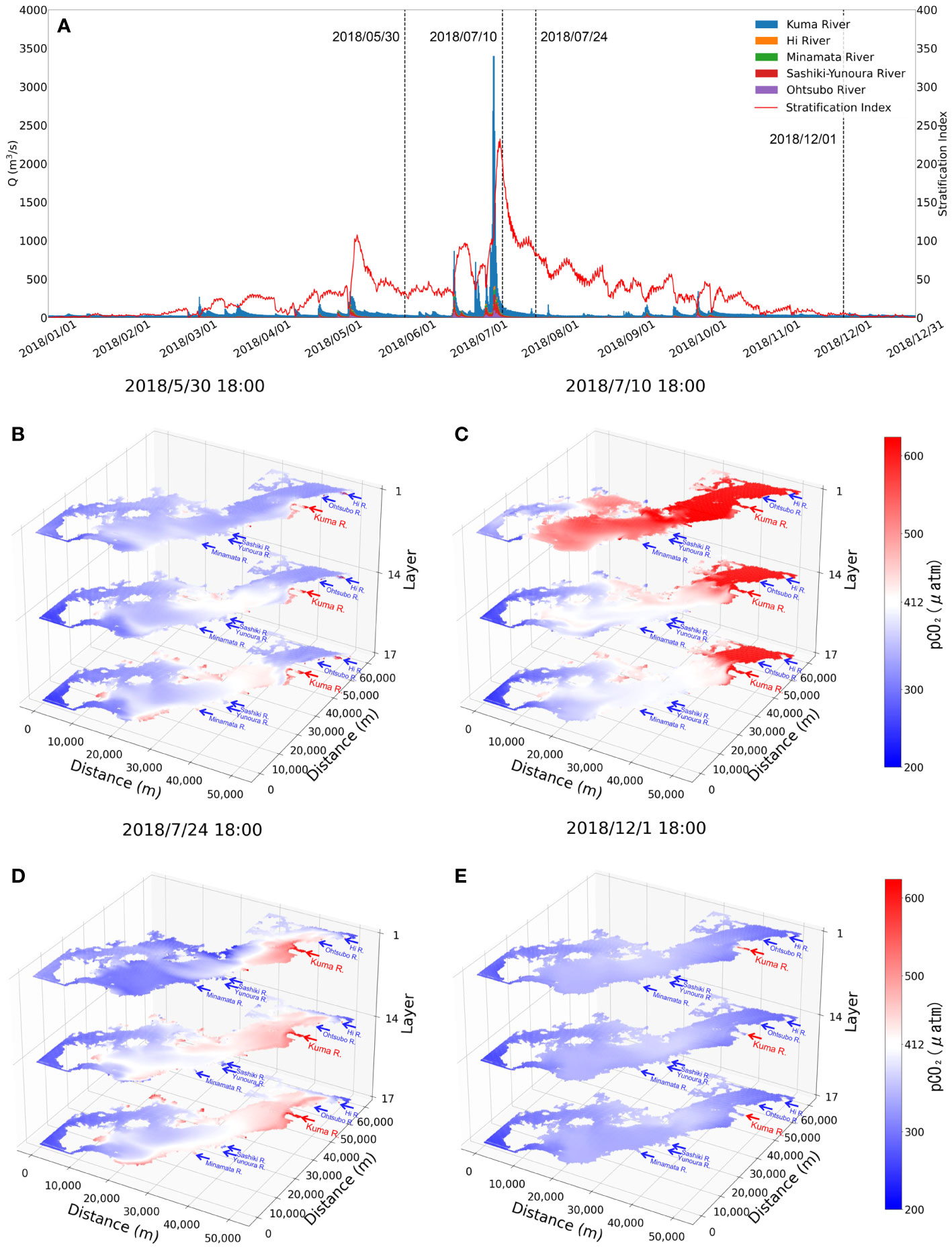
Figure 4 Comparison plots of the flow rate of the rivers flowing into the Yatsushiro Sea in 2018 and stratification index (A) and the horizontal distribution of pCO₂ for the four periods (B–E).

The horizontal pCO₂ distribution of the bay is shown in Figure 4B for several more typical periods—namely, the period before the massive flooding of the Kuma River in July 2018 when it was less affected by freshwater inflow (30 May 2018), the period one week after the flooding (10 July 2018), the period three weeks after the flooding (24 July 2018), and the dry winter period (1 December 2018). The x- and y-axes in this figure represent the distance, while the z-axis represents the position in the σ coordinate system in a total of 17 layers. According to the vertical resolution of the model, the 1st and 17th layers are the surface and bottom layers of the water body, respectively, while the 14th layer is the part that accounts for 45% to 55% of the total water depth, which is considered to be the middle part of the water body.

As we can see, the density stratification peaks (9 July 2018, 18:00:00, SI = 232.26) about a week after the influx of large amounts of freshwater into the bay (Figure 4C). At the same time, with the higher CO₂ concentration freshwater covering the surface of the seawater, the average pCO₂ concentration of the whole bay reaches a peak (surface pCO_2avg = 726.31 μatm). The bay during this period exhibits a source of atmospheric CO₂ mainly due to the freshwater inflow.

After another two weeks or so, we can see that the pCO₂ in the surface layer drops to a lower level (24 July 2018, 18:00, surface pCO_2avg = 357.34 μatm), with only some high pCO₂ remaining in the surface water near the estuary. In the middle and bottom layers, however, the pCO₂ is higher than that in the surface layer. The main effect of stratification at that time is to inhibit the upwelling of water with a higher level of pCO₂ in the bottom layer to the surface layer, combined with photosynthesis by phytoplankton in surface seawater, resulting in a sink of seawater for atmospheric CO₂. In addition, we found that the pCO₂ in the central part of the bay (the region between distance from 20 to 40 km of the y-axis in Figure 4) is always slightly higher than that in the southern and northern parts during the periods less affected by freshwater inflow (Figure 4B, E). The main reasons for this phenomenon are, on the one hand, that the south and the north are farther away from the Kuma River than the central part, which makes the impact of freshwater less. On the other hand, that the south is connected to the outer sea through the strait, while the north is connected to the Ariake Sea, which makes it easier for these two areas to reduce the impact of freshwater with high pCO₂ through seawater exchange.

The vertical dynamics of the two sites before and after the flooding period with time are shown in Figure 5. pCO₂ and phytoplankton biomass are examined. The two sites are St.13, near the estuary of the Kuma River (Figures 5A–C), and St.18, located in the southern part of the bay, far from the estuary (Figures 5D–F).

FIGURE 5

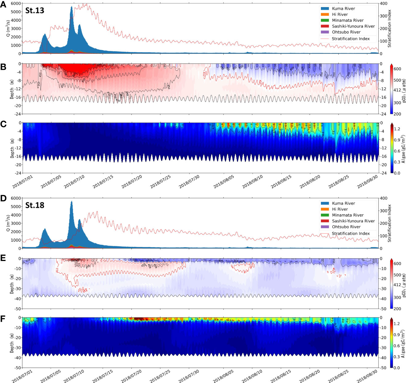
Figure 5 Comparison of the flow rate of the rivers flowing into the Yatsushiro Sea and stratification index (A, D), pCO₂ distribution (B, E), and algae biomass distribution (C, F) at St.13 (A–C) and St.18 (D–F) from 1 July 2018 to 1 September 2018.

By the distribution of phytoplankton biomass in St.18 (Figure 5C), we found that the phytoplankton biomass in this area was much higher around two weeks after the flood than before. In contrast, St.13 had a late start of phytoplankton proliferation due to the influence of freshwater residues. We suggest that during the period after the large-scale freshwater inflow, the bay was subjected to nutrient input from terrestrial sources, leading to a large phytoplankton bloom and thus making the period exhibit a strong sink of atmospheric CO₂. This also resulted in the surface pCO₂ concentrations in most areas of the Yatsushiro Sea during this period (St.18, 24 July 2018, 18:00, surface pCO₂ = 307.83 μatm) (Figure 4D) being even lower than those before the flood (St.18, 30 May 2018 18:00, surface pCO₂ = 376.61 μatm) (Figure 4B) and during the dry period (St.18, 24 July 2018 18:00, surface pCO₂ = 352.54 μatm) (Figure 4E), except near the estuary.

At St.13, the influence of freshwater lasted for a long time, resulting in the surface pCO₂ (surface pCO_2avg = 539.94 μatm) being higher than the atmospheric pCO₂ (412 μatm) for about 40 days starting from June 20. However, at St.18, which is farther from the estuary, the surface layer pCO₂ decreased to a level below atmospheric pCO₂ only about 10 days after the surface layer was covered by freshwater with a high pCO₂ concentration. The surface pCO₂ concentration at this point reached the lowest value (257.82 μatm) at 17:00 on 20 July 2018, which was much lower than that of the middle layer (441.96 μatm) and the bottom layer (360.08 μatm), showing an apparent layered state.

3.5 Correlation between Surface pCO₂ and Stratification

Since stratification in the Yatsushiro Sea is mainly caused by freshwater inflow from the Kuma River, which in turn largely increases the pCO₂ concentration in the surface layer, it is difficult to evaluate the relationship between stratification and pCO₂ dynamics in isolation while ignoring the amount of pCO₂ increase caused by freshwater inflow.

The correlation plot between SI and surface pCO₂ from 1 February 2018 to 31 December 2018 is displayed in Figure 6A. As this simulation started on 1 January 2018, it took about 30 days for the simulated values to reach a more accurate value, so only the results after February 1 are analyzed here. The results show that the surface pCO₂ of St.13 had a strong positive correlation with SI over nearly one full year (r = 0.87), while St.18, which is farther away from the estuary, did not show a significant correlation (r = 0.25). We speculate that this result may be due to the strength and duration of the freshwater influence.

FIGURE 6

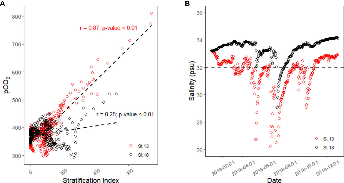
Figure 6 Linear correlation between surface pCO₂ and stratification index (A) and surface salinity of St.13 and St.18 in 2018 (B).

The value of salinity in seawater can be used as an indicator of the influence of freshwater. Figure 6B shows the trend of the surface salinity values of St.13 and St.18 in 2018. We used a salinity value of 32 psu as a cut-off, and we considered a salinity below 32 psu as being more strongly influenced by freshwater. From this figure, we know that St.13 is under a strong freshwater influence for most of the year, except for the dry winter period (mid-October to mid-January). St.18 is only about 25 days after the massive flood in July, when the salinity was below 32 psu.

We divided St.18 into a freshwater-influenced period (7/7 to 7/29), freshwater-abated period (7/29 to 10/17), and dry period (10/18 to 12/31) according to the strength of the freshwater influence in order to explore the factors affecting surface pCO₂ separately. In addition to the relationship between SI and pCO₂, we also analyzed the correlation between water temperature, DIC, and algae together, where all the values except SI were surface values. The results are displayed in Figure 7.

FIGURE 7

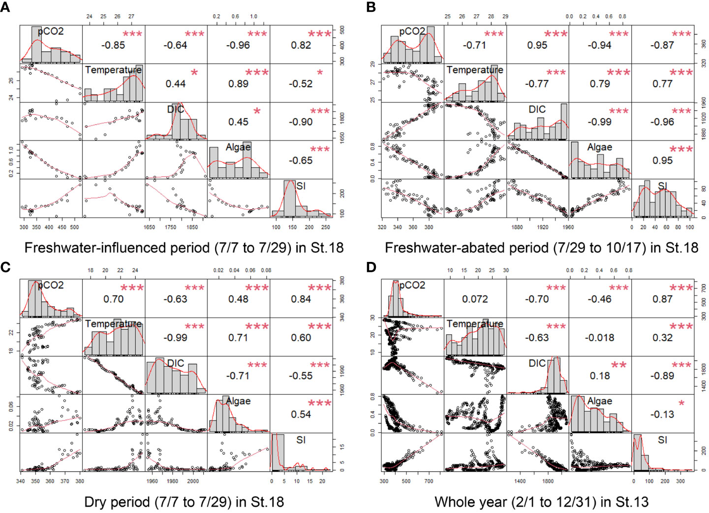
Figure 7 Multiple linear regression (Pearson’s correlation coefficients and p-values) (* p ≤ 0.05, ** p ≤ 0.01, *** p ≤ 0.001) at different periods of St.13 (D) and St.18 (A–C). The items involved in the analysis were pCO₂, water temperature, salinity, DIC, TA, algae, and SI.

During the freshwater-influenced period (Figure 7A), the density stratification of St.18 was highly developed (SI > 100), with pCO₂ showing a strong positive correlation with SI (r = 0.82). During the freshwater-abated period (Figure 7B), St.18 maintained a strong stratification (SI > 80) in the first half of the period and the SI had a strong negative correlation with pCO₂ (r = −0.87). During the dry period (Figure 7C), although pCO₂ showed a strong positive correlation with SI (r = 0.84), the effect of SI on pCO₂ was very limited due to the very weak stratification during this period (SI< 10). In addition, regardless of the period, we found that surface DIC was negatively correlated with SI and showed a solidly negative correlation (r< −0.9) in the more stratified periods (Figures 7A, B). They had a strong negative correlation (r = −0.89) even throughout the whole year of St.13. In general, it can be concluded that in stratified waters, stratification is the main factor affecting pCO₂ in surface waters, with a positive correlation occurring during the freshwater-influenced period and a negative correlation occurring during the freshwater-abated period.

The natural fluctuation of pCO₂ in coastal water is related to biological processes such as respiration and photosynthesis (Shamberger et al., 2011; Buapet et al., 2013; Saderne et al., 2013; Edman and Anderson, 2014). In contrast, during periods of oligotrophy and low seawater temperatures, when biological activity is suppressed due to insufficient nutrient supply or low-temperature conditions, the temperature is likely to be the main factor affecting the distribution of pCO₂ in the water column (Bates et al., 1998; Borges et al., 2006). In general, phytoplankton in the surface layer reduces pCO₂ through photosynthesis—for example, from July to October when stratification is strong (Figures 7A, B), both showed very strong negative correlations (r = −0.96 and r = −0.94). However, the correlation between phytoplankton and pCO₂ was not significant for other periods, partly because of the low number of phytoplankton and partly because phytoplankton in the water column provide easily degradable organic carbon through respiration over time. The increase in temperature between July and October reduced pCO₂, which was strongly related to the influx of nutrients. Phytoplankton proliferated rapidly and had more intense biological processes under the combined effect of high nutrient levels and suitable temperatures. After October, the water temperature changed to a strong positive correlation with pCO₂ (r = 0.7).

3.6 CO2 flux of the Yatsushiro sea

From the results of the air–water CO₂ exchange fluxes by month (Figure 8), the response of F_CO2 to stratification and freshwater inflow varies depending on the distance from the estuary of the Kuma River. The A2 area, because it is located near the estuary, always has the highest absolute value of F_CO2, regardless of whether it is in the absorption or emission phase. A4 area is a sink for atmospheric CO₂ at all times of the year because it is the furthest from the estuary and can easily exchange seawater with the outer ocean.

FIGURE 8

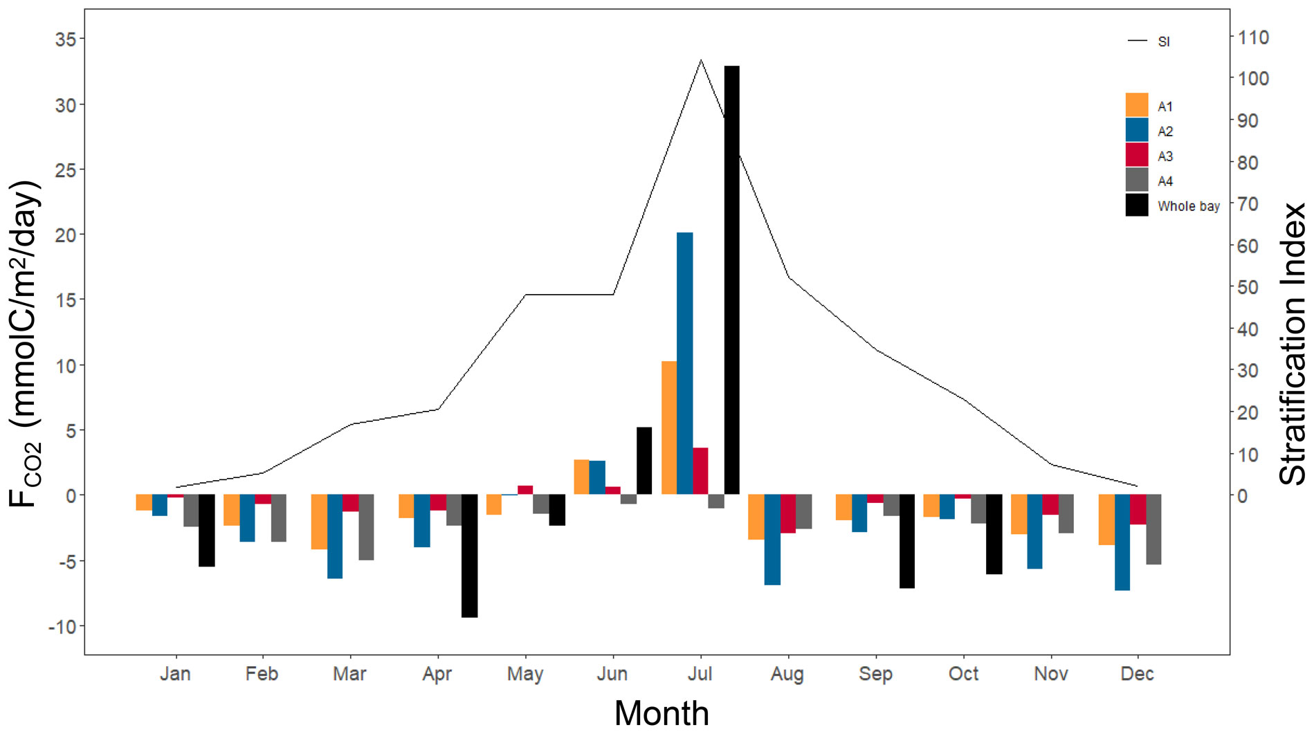
Figure 8 Monthly air–water CO₂ fluxes for the four areas and the whole bay (A1 to A4, Whole bay), and the stratification index of the Yatsushiro Sea.

From the numerical results, the highest CO₂ release flux (19.47 mmol/m²/day) is at A2 in July, while the highest absorption (−7.11 mmol/m²/day) is at A2 in December. It can be seen that the Yatsushiro Sea is a sink area for atmospheric CO₂ (−1.7 mmol/m²/day) throughout the year, except for June and July, when there is a large inflow of freshwater, which is the source of atmospheric CO₂. Even in the A4 area, which is the least affected by freshwater and closest to the outer sea, its sink intensity decreases to very low in June and July (−0.73 and −1.04 mmol/m²/day). This result shows that freshwater inflow plays a critical role in influencing the F_CO2 of the bay. Due to the respiration of terrestrial organic carbon and the terrestrial input of freshwater CO₂, most inland waters and estuaries are substantial CO₂ contributors to the atmosphere (Borges and Abril, 2011; Chen et al., 2013; Raymond et al., 2013; Hotchkiss et al., 2015). The Yatsushiro Sea, on the other hand, experiences relatively less influence from human activities (the population of the basin is 170,000), which may result in the bay having biogeochemical processes that are more distinct from them, leading to the bay being a sink for atmospheric CO₂ throughout the year.

In this work, we only estimated the flux of air-water CO₂ exchange in the whole Yatsushiro Sea with the simplified ecological model developed this time, and did not quantify the flux of CO₂ within the water column. It is expected that, like other shallow coastal waters where blue carbon ecosystems grow, in the Yatsushiro Sea, most of the CO₂ that sinks into the seawater will be absorbed and fixed in the sediment by the biological processes of blue carbon ecosystems such as seagrass beds, corals and marine phytoplankton. In addition, the lateral carbon fluxes between the Yatsushiro Sea and the outer sea are of equal interest. Continuing field measurements of CO₂ dynamics and blue carbon ecosystems in the Yatsushiro Sea in subsequent studies, coupling the effects of higher ecosystems such as seagrass beds and coral reefs into this ecological model as well, continuing to optimize the accuracy of the model and attempting to quantify carbon fluxes within the Yatsushiro Sea taking into account stratification effects is essential to further understand the contribution of stratified shallow coastal waters with growing blue carbon ecosystems to the reduction of atmospheric CO₂.

4 Conclusions

In this study, we chose the Yatsushiro Sea, where CO₂ dynamics have never been studied before to conduct the first field measurements of CO₂ dynamics. We found that pCO₂ is stratified in the vertical direction with density stratification at the estuary of the Kuma River.

Based on the field measurement results, we considering the influence of stratification, developed a high-resolution 3D hydrodynamic-ecological numerical model that can accurately reproduce the CO₂ dynamics of the estuary area of the Kuma River, then extended the application of the ecological model by coupling it with the hydrodynamic model that can also well reproduce the CTD profiles and the mixing states of the whole Yatsushiro Sea. In terms of the hydrodynamic module, the model not only fits the estuarine measurement results very well (d_ref > 0.6) but also performs very well in the calculations for the whole domain of the bay (d_ref between 0.18 and 0.92). In addition, the fit of the parameter SI, which evaluates the strength of water density stratification, also has an excellent performance (d_ref between 0.23 and 0.76). In the ecological module, the model can basically reproduce the CO₂ dynamics in the estuary region of the Kuma River (d_ref > 0.6), and more measured CO₂ dynamics data are needed to improve the model on CO₂ dynamics of the whole bay. Also, the biological processes are still need to be improved in subsequent studies.

Using this model, we simulated the CO₂ dynamics of the bay in 2018 and preliminary analyzed the interaction between seawater CO₂ dynamics and stratification in the bay. The results show that the CO₂ dynamics of the bay has substantial fluctuations in both the horizontal and vertical directions. Depending on the distance from the estuary and the outer sea in the horizontal direction, the surface pCO₂ varies greatly depending on the strength and duration of the freshwater influence. In the vertical direction, stratification strongly contributes to the maintenance of high pCO₂ concentrations in the surface water during the freshwater influence period. During the dissipation period of freshwater influence, stratification causes the pCO₂ concentration in the surface water to be much lower than that in the middle and bottom of the water.

Finally, we used the model to estimate the annual pattern of F_CO2 in the bay in 2018. The results show that the Yatsushiro Sea becomes a source of atmospheric CO₂ in June and July when the freshwater inflow is high and a sink of atmospheric CO₂ at all other times. And the Yatsushiro Sea was a sink area for atmospheric CO₂ in 2018 (−1.70 mmol/m²/day).

Data availability statement

The original contributions presented in the study are included in the article/Supplementary Material. Further inquiries can be directed to the corresponding author.

Author contributions

Conceptualization, methodology and writing—original draft preparation: BX and SY. Writing—review and check: SY, KK, and KN. Field measurements: BX, SY, NS, and HK. Numerical model development: BX, NS, BC, and LH. All authors have read and agreed to the published version of the manuscript. All authors contributed to the article and approved the submitted version.

Funding

This research was funded by JSPS KAKENHI Grant NumberJP18H01545, JP22K18832, JP22H01601 and by JST SPRING Grant Number JPMJSP2136.

Acknowledgments

This work was supported by the JSPS KAKENHI GrantNumber JP18H01545, JP22K18832 and JP22H01601, and by JST SPRING Grant NumberJPMJSP2136. The authors would like to express theirprofound thanks.

Conflict of interest

Author BX was employed by Guangzhou Municipal Group Co., Ltd.

The remaining authors declare that the research was conducted in the absence of any commercial or financial relationships that could be construed as a potential conflict of interest.

Publisher’s note

All claims expressed in this article are solely those of the authors and do not necessarily represent those of their affiliated organizations, or those of the publisher, the editors and the reviewers. Any product that may be evaluated in this article, or claim that may be made by its manufacturer, is not guaranteed or endorsed by the publisher.

Supplementary material

The Supplementary Material for this article can be found online at: https://www.frontiersin.org/articles/10.3389/fmars.2022.991802/full#supplementary-material

Supplementary Figure 1 | Hydrodynamic model validation (tide level), (A) for Misumi Observatory, (B) for Yatsushiro Observatory.

Supplementary Figure 2 | Comparison of contour plots of σt (A, B), salinity (C, D), and water temperature (E, F) for each mixing state at the measurement point ((1) in Figure 1) located at the estuary of the Kuma River. Measurement results (top, (A, C, E)) and numerical model results (bottom, (B, D, F)).

Supplementary Figure 3 | Comparison of contour plots of DIC (A, B), TA (C, D), and pCO2 (E, F) for each mixing state at the measurement point ((1) in Figure 1) located at the estuary of the Kuma River. Measurement results (top, (A, C, E)) and numerical model results (bottom, (B, D, F)).

Supplementary Figure 4 | Comparison of σt (A), salinity (B), and water temperature (C) at surface layer (A-1, B-1, C-1) and bottom layer (A-2, B-2, C-2) between the simulation and field measurement at each station (St.11 to St.19 are the results of each station respectively).

Supplementary Figure 5 | Comparison of contour plots of σt (A, B), salinity (C, D), and water temperature (E, F) for each mixing state at each point located on the central line of the Yatsushiro Sea (St.11 to St19 in Figure 1). Measurement results (top, (A, C, E)) and numerical model results (bottom, (B, D, F)).

Supplementary Figure 6 | Comparison of stratification index between the simulation and field measurement at each station (St.11 to St.19 are the results of each station respectively).

References

Alongi D. M., Murdiyarso D., Fourqurean J. W., Kauffman J. B., Hutahaean A., Crooks S., et al. (2016). Indonesia’s blue carbon: a globally significant and vulnerable sink for seagrass and mangrove carbon. Wetlands Ecol. Manage. 24 (1), 3–13. doi: 10.1007/s11273-015-9446-y

CrossRef Full Text | Google Scholar

Alosairi Y., Alsulaiman N. (2019). Hydro-environmental processes governing the formation of hypoxic parcels in an inverse estuarine water body: Model validation and discussion. Mar. pollut. Bull. 144, 92–104. doi: 10.1016/j.marpolbul.2019.04.067

PubMed Abstract | CrossRef Full Text | Google Scholar

Arakawa H., Kanda Y., Ishihara T. (2007). Prediction of Sea surface wind distribution with a three dimensional wind model. Proc. OF Coast. ENGINEERING JSCE 54, 131–135. doi: 10.2208/proce1989.54.131

CrossRef Full Text | Google Scholar

Bakker D. C. E., de Baar H. J. W., de Jong E. (1999). The dependence on temperature and salinity of dissolved inorganic carbon in East Atlantic surface waters. Mar. Chem. 65 (3), 263–280. doi: 10.1016/S0304-4203(99)00017-1

CrossRef Full Text | Google Scholar

Bates N. R., Takahashi T., Chipman D. W., Knap A. H. (1998). Variability of pCO2 on diel to seasonal timescales in the Sargasso Sea near Bermuda. J. Geophys. Res. 103(C8), 15567–15585. doi: 10.1029/98JC00247.

CrossRef Full Text | Google Scholar

Bauer J. E., Cai W.-J., Raymond P. A., Bianchi T. S., Hopkinson C. S., Regnier P. A. G. (2013). The changing carbon cycle of the coastal ocean. Nature 504 (7478), 61–70. doi: 10.1038/nature12857

PubMed Abstract | CrossRef Full Text | Google Scholar

Blauw A. N., Los H. F. J., Bokhorst M., Erftemeijer P. L. A. (2008). GEM: a generic ecological model for estuaries and coastal waters. Hydrobiologia 618 (1), 175–175. doi: 10.1007/s10750-008-9575-x

CrossRef Full Text | Google Scholar

Boldrin A., Carniel S., Giani M., Marini M., Bernardi Aubry F., Campanelli A., et al. (2009). Effects of bora wind on physical and biogeochemical properties of stratified waters in the northern Adriatic. J. Geophysical Research: Oceans 114, C08S92. doi: 10.1029/2008JC004837

CrossRef Full Text | Google Scholar

Borges A. V., Abril G. (2011). 5.04 - carbon dioxide and methane dynamics in estuaries. Eds. Wolanski E., McLusky D., Coastal S. (Waltham: Academic Press), 119–161.

Google Scholar

Borges A. V., Schiettecatte L.-S., Abril G., Delille B., Gazeau F. (2006). Carbon dioxide in European coastal waters. Estuarine Coast. Shelf Sci. 70, 375–387. doi: 10.1016/j.ecss.2006.05.046

CrossRef Full Text | Google Scholar

Buapet P., Gullström M., Björk M. (2013). Photosynthetic activity of seagrasses and macroalgae in temperate shallow waters can alter seawater pH and total inorganic carbon content at the scale of a coastal embayment. Mar. Freshw. Res. 64 (11), 1040–1048. doi: 10.1071/MF12124

CrossRef Full Text | Google Scholar

Chen C. T. A., Huang T. H., Chen Y. C., Bai Y., He X., Kang Y. (2013). Air–sea exchanges of CO2 in the world's coastal seas. Biogeosciences 10 (10), 6509–6544. doi: 10.5194/bg-10-6509-2013

CrossRef Full Text | Google Scholar

Chen Z., Huang P., Zhang Z. (2019). Interaction between carbon dioxide emissions and eutrophication in a drinking water reservoir: A three-dimensional ecological modeling approach. Sci. Total Environ. 663, 369–379. doi: 10.1016/j.scitotenv.2019.01.336

PubMed Abstract | CrossRef Full Text | Google Scholar

Chen C.-T. A., Zhai W., Dai M. (2008). Riverine input and air–sea CO2 exchanges near the changjiang (Yangtze river) estuary: Status quo and implication on possible future changes in metabolic status. Continental Shelf Res. 28 (12), 1476–1482. doi: 10.1016/j.csr.2007.10.013

CrossRef Full Text | Google Scholar

Deltares (2017). Delft3D-FLOW users' manual; simulation of multi-dimensional hydrodynamic flows and transport phenomena, including sediments. version: 3.15 (The Netherlands: Deltares, Delft).

Google Scholar

Deltares (2018). Delft3D functional specifications. (The Netherlands: Deltares, Delft) 46–46.

Google Scholar

Donato D. C., Kauffman J. B., Murdiyarso D., Kurnianto S., Stidham M., Kanninen M. (2011). Mangroves among the most carbon-rich forests in the tropics. Nat. Geosci. 4 (5), 293–297. doi: 10.1038/ngeo1123

CrossRef Full Text | Google Scholar

Duarte C. M., Marbà N., Gacia E., Fourqurean J. W., Beggins J., Barrón C., et al. (2010). Seagrass community metabolism: Assessing the carbon sink capacity of seagrass meadows. Global Biogeochemical Cycles 24, GB4032. doi: 10.1029/2010GB003793

CrossRef Full Text | Google Scholar

Duarte C. M., Middelburg J. J., Caraco N. (2005). Major role of marine vegetation on the oceanic carbon cycle. Biogeosciences 2 (1), 1–8. doi: 10.5194/bg-2-1-2005

CrossRef Full Text | Google Scholar

Edman M. K., Anderson L. G. (2014). Effect on pCO2 by phytoplankton uptake of dissolved organic nutrients in the central and northern Baltic Sea, a model study. J. Mar. Syst. 139, 166–182. doi: 10.1016/j.jmarsys.2014.06.004

CrossRef Full Text | Google Scholar

Eyre B. D. (2000). “Regional evaluation of nutrient transformation and phytoplankton growth in nine river-dominated sub-tropical east Australian estuaries,” in Marine ecology progress series. 205, 61–83. doi: 10.3354/meps205061

CrossRef Full Text | Google Scholar

Falkowski P. G., Raven J. A. (2013). Aquatic photosynthesis: (Second Edition). (Princeton: Princeton University Press).

Google Scholar

Fourqurean J. W., Duarte C. M., Kennedy H., Marbà N., Holmer M., Mateo M. A., et al. (2012). Seagrass ecosystems as a globally significant carbon stock. Nat. Geosci. 5 (7), 505–509. doi: 10.1038/ngeo1477

CrossRef Full Text | Google Scholar

Golterman H. (1982). Reviewed work: Aquatic chemistry. an introduction emphasizing chemical equilibria in natural waters. J. Ecol. 70 (3), 924–925. doi: 10.2307/2260132

CrossRef Full Text | Google Scholar

Gurel M., Tanik A., Gonec E., Russo R. C. (2005). Biogeochemical Cycles. In: Wolflin J. P., Gonenc I. E, eds. Coastal Lagoons. s.l.: CRC Press

Google Scholar

Hao L., Sato Y., Yano S., Xiong B., Chi B. (2021). Effects of Large-scale effluent of the chikugo river due to 2020 Kyushu floods on the development of hypoxia in the ariake Sea. J. Japan Soc. Civil Engineers Ser. B2 (Coastal Engineering) 77, I_865–I_870. doi: 10.2208/kaigan.77.2_I_865

CrossRef Full Text | Google Scholar

Hartnett H. E., Keil R. G., Hedges J. I., Devol A. H. (1998). Influence of oxygen exposure time on organic carbon preservation in continental margin sediments. Nature 391 (6667), 572–575. doi: 10.1038/35351

CrossRef Full Text | Google Scholar

Hotchkiss E. R., Hall R. O. Jr., Sponseller R. A., Butman D., Klaminder J., Laudon H., et al. (2015). Sources of and processes controlling CO 2 emissions change with the size of streams and rivers. Nat. Geosci. 8, 696–699. doi: 10.1038/ngeo2507

CrossRef Full Text | Google Scholar

Howard J. L., Creed J. C., Aguiar M. V. P., Fourqurean J. W. (2018). CO2 released by carbonate sediment production in some coastal areas may offset the benefits of seagrass “Blue carbon” storage. Limnology Oceanography 63 (1), 160–172. doi: 10.1002/lno.10621

CrossRef Full Text | Google Scholar

Howard J., Sutton-Grier A., Herr D., Kleypas J., Landis E., McLeod E., et al. (2017). Clarifying the role of coastal and marine systems in climate mitigation. Front. Ecol. Environ. 15 (1), 42–50. doi: 10.1002/fee.1451

CrossRef Full Text | Google Scholar

Howarth R., Chan F., Conley D. J., Garnier J., Doney S. C., Marino R., et al. (2011). Coupled biogeochemical cycles: eutrophication and hypoxia in temperate estuaries and coastal marine ecosystems. Front. Ecol. Environ. 9 (1), 18–26. doi: 10.1890/100008

CrossRef Full Text | Google Scholar

Ishizaki H., Mitsuta Y. (1962). On the scale of peak gust and the gust factor. Disaster Prev. Res. Inst. Annu. 5, 135–138. Available at: https://www.dpri.kyoto-u.ac.jp/nenpo/no05/05a0/a05a0p15.pdf

Google Scholar

Koho K. A., Nierop K. G. J., Moodley L., Middelburg J. J., Pozzato L., Soetaert K., et al. (2013). Microbial bioavailability regulates organic matter preservation in marine sediments. Biogeosciences 10 (2), 1131–1141. doi: 10.5194/bg-10-1131-2013

CrossRef Full Text | Google Scholar

Koné Y. J. M., Abril G., Kouadio K. N., Delille B., Borges A. V. (2009). Seasonal variability of carbon dioxide in the rivers and lagoons of ivory coast (West Africa). Estuaries Coasts 32 (2), 246–260. doi: 10.1007/s12237-008-9121-0

CrossRef Full Text | Google Scholar

Kubo A., Maeda Y., Kanda J. (2017). A significant net sink for CO2 in Tokyo bay. Sci. Rep. 7 (1), 44355–44355. doi: 10.1038/srep44355

PubMed Abstract | CrossRef Full Text | Google Scholar

Kuwae T., Kanda J., Kubo A., Nakajima F., Ogawa H., Sohma A., et al. (2016). Blue carbon in human-dominated estuarine and shallow coastal systems. Ambio 45 (3), 290–301. doi: 10.1007/s13280-015-0725-x

PubMed Abstract | CrossRef Full Text | Google Scholar

Lavigne H., Gattuso J. (2010). Seacarb: seawater carbonate chemistry with R. R package version 2.4.10. Available at: http://CRAN.R-project.org/package=seacarb

Google Scholar

Le Quéré C., Andrew R. M., Canadell J. G., Sitch S., Korsbakken J. I., Peters G. P., et al. (2016). Global carbon budget 2016. Earth Syst. Sci. Data 8 (2), 605–649. doi: 10.5194/essd-8-605-2016

CrossRef Full Text | Google Scholar

Lesser G. R., Roelvink J. A., van Kester J. A. T. M., Stelling G. S. (2004). Development and validation of a three-dimensional morphological model. Coast. Eng. 51, 883–915. doi: 10.1016/j.coastaleng.2004.07.014

CrossRef Full Text | Google Scholar

Lo Iacono C., Mateo M. A., Gràcia E., Guasch L., Carbonell R., Serrano L., et al. (2008). Very high-resolution seismo-acoustic imaging of seagrass meadows (Mediterranean sea): Implications for carbon sink estimates. Geophysical Res. Lett. 35 (18), L18601. doi: 10.1029/2008GL034773

CrossRef Full Text | Google Scholar

Macreadie P. I., Serrano O., Maher D. T., Duarte C. M., Beardall J. (2017). Addressing calcium carbonate cycling in blue carbon accounting. Limnology Oceanography Lett. 2 (6), 195–201. doi: 10.1002/lol2.10052

CrossRef Full Text | Google Scholar

Maher D. T., Eyre B. D. (2012). Carbon budgets for three autotrophic Australian estuaries: Implications for global estimates of the coastal air-water CO2 flux. Global Biogeochemical Cycles 26, GB1032. doi: 10.1029/2011GB004075

CrossRef Full Text | Google Scholar

McKee K. L., Cahoon D. R., Feller I. C. (2007). Caribbean Mangroves adjust to rising sea level through biotic controls on change in soil elevation. Global Ecol. Biogeography 16 (5), 545–556. doi: 10.1111/j.1466-8238.2007.00317.x

CrossRef Full Text | Google Scholar

McLeod E., Chmura G. L., Bouillon S., Salm R., Björk M., Duarte C. M., et al. (2011). A blueprint for blue carbon: Toward an improved understanding of the role of vegetated coastal habitats in sequestering CO2. Front. Ecol. Environ. 9, 552–560. doi: 10.1890/110004

CrossRef Full Text | Google Scholar

Menshutkin V. V., Rukhovets L. A., Filatov N. N. (2014). Ecosystem modeling of freshwater lakes (review): 2. models of freshwater lake’s ecosystem. Water Resour. 41 (1), 32–45. doi: 10.1134/S0097807814010084

CrossRef Full Text | Google Scholar

Murdiyarso D., Purbopuspito J., Kauffman J. B., Warren M. W., Sasmito S. D., Donato D. C., et al. (2015). The potential of Indonesian mangrove forests for global climate change mitigation. Nat. Climate Change 5 (12), 1089–1092. doi: 10.1038/nclimate2734

CrossRef Full Text | Google Scholar

Nakayama K., Komai K., Tada K., Lin H. C., Yajima H., Yano S., et al. (2020). Modeling dissolved inorganic carbon considering submerged aquatic vegetation. Ecol. Model. 431, 109188. doi: 10.1016/j.ecolmodel.2020.109188

CrossRef Full Text | Google Scholar

Nellemann C., Corcoran E., Duarte E, Valdes M., DeYoung L., Fonseca C., et al (2009). Blue carbon. A rapid response assessment. Birkeland: UNEP, GRID-Arendal, Bikeland Trykkeri A.S. 78 p.

Google Scholar

Niu L., van Gelder P., Zhang C., Guan Y., Vrijling J. K. (2016). Physical control of phytoplankton bloom development in the coastal waters of jiangsu (China). Ecol. Model. 321, 75–83. doi: 10.1016/j.ecolmodel.2015.10.008

CrossRef Full Text | Google Scholar

Raven J. A., Falkowski P. G. (1999). Oceanic sinks for atmospheric CO2. Plant Cell Environ. 22, 741–755. doi: 10.1046/j.1365-3040.1999.00419.x

CrossRef Full Text | Google Scholar

Raymond P. A., Hartmann J., Lauerwald R., Sobek S., McDonald C., Hoover M., et al. (2013). Global carbon dioxide emissions from inland waters. Nature 503 (7476), 355–359. doi: 10.1038/nature12760

PubMed Abstract | CrossRef Full Text | Google Scholar

Saderne V., Fietzek P., Herman P. M. J. (2013). Extreme variations of pCO2 and pH in a macrophyte meadow of the Baltic Sea in summer: Evidence of the effect of photosynthesis and local upwelling. PLoS One 8 (4), e62689–e62689. doi: 10.1371/journal.pone.0062689

PubMed Abstract | CrossRef Full Text | Google Scholar

Shamberger K. E. F., Feely R. A., Sabine C. L., Atkinson M. J., DeCarlo E. H., Mackenzie F. T., et al. (2011). Calcification and organic production on a Hawaiian coral reef. Mar. Chem. 127, 64–75. doi: 10.1016/j.marchem.2011.08.003

CrossRef Full Text | Google Scholar

Shim J., Kim D., Kang Y. C., Lee J. H., Jang S.-T., Kim C.-H. (2007). Seasonal variations in pCO2 and its controlling factors in surface seawater of the northern East China Sea. Continental Shelf Res. 27 (20), 2623–2636. doi: 10.1016/j.csr.2007.07.005

CrossRef Full Text | Google Scholar

Simpson J. H., Brown J., Matthews J., Allen G. (1990). Tidal straining, density currents, and stirring in the control of estuarine stratification. Estuaries 13 (2), 125–132. doi: 10.2307/1351581

CrossRef Full Text | Google Scholar

Sohma A., Shibuki H., Nakajima F., Kubo A., Kuwae T. (2018). Modeling a coastal ecosystem to estimate climate change mitigation and a model demonstration in Tokyo bay. Ecol. Model. 384, 261–289. doi: 10.1016/j.ecolmodel.2018.04.019

CrossRef Full Text | Google Scholar

Sonoda Y., Takikawa K., Kawasaki S., Aoyama C., Saito T. (2013). CHARACTERISTICS OF WATER QUALITY ENVIRONMENT IN THE YATSUSHIRO SEA AREA. J. Japan Soc. Civil Engineers Ser. B3 (Ocean Engineering) 69, I_1240–I_1245. doi: 10.2208/jscejoe.69.I_1240

CrossRef Full Text | Google Scholar

Sylaios G., Tsihrintzis V., Haralambidou K. (2006). Modeling stratification – mixing processes at the mouth of a dam – controlled river. European Water 13(14), 21–28. Available at: https://www.ewra.net/ew/pdf/EW_2006_13-14_03.pdf.

Google Scholar

Tadokoro M., Yano S. (2019). EVALUATION OF EFFECTS OF TEMPERATURE AND RIVER DISCHARGE CHANGES DUE TO CLIMATE CHANGE ON HYPOXIA IN THE ARIAKE SEA. J. Japan Soc. Civil Engineers Ser. B2 (Coastal Engineering) 75, I_1231–I_1236. doi: 10.2208/kaigan.75.I_1231

CrossRef Full Text | Google Scholar

Tokoro T., Hosokawa S., Miyoshi E., Tada K., Watanabe K., Montani S., et al. (2014). Net uptake of atmospheric CO2 by coastal submerged aquatic vegetation. Global Change Biol. 20 (6), 1873–1884. doi: 10.1111/gcb.12543

CrossRef Full Text | Google Scholar

Verspagen J. M. H., Van de Waal D. B., Finke J. F., Visser P. M., Van Donk E., Huisman J. (2014). Rising CO2 levels will intensify phytoplankton blooms in eutrophic and hypertrophic lakes. PLoS One 9 (8), e104325–e104325. doi: 10.1371/journal.pone.0104325

PubMed Abstract | CrossRef Full Text | Google Scholar

Wakeham S. G., Howes B. L., Dacey J. W. H., Schwarzenbach R. P., Zeyer J. (1987). Biogeochemistry of dimethylsulfide in a seasonally stratified coastal salt pond. Geochimica Cosmochimica Acta 51 (6), 1675–1684. doi: 10.1016/0016-7037(87)90347-4

CrossRef Full Text | Google Scholar

Wang S.-y., Zhai W.-d. (2021). Regional differences in seasonal variation of air–sea CO2 exchange in the yellow Sea. Continental Shelf Res. 218, 104393. doi: 10.1016/j.csr.2021.104393

CrossRef Full Text | Google Scholar

Wanninkhof R. (1992). Relationship between wind speed and gas exchange over the ocean. J. Geophysical Research: Oceans 97 (C5), 7373–7382. doi: 10.1029/92JC00188

CrossRef Full Text | Google Scholar

Weiss R. F. (1974). Carbon dioxide in water and seawater: the solubility of a non-ideal gas. Mar. Chem. 2 (3), 203–215. doi: 10.1016/0304-4203(74)90015-2

CrossRef Full Text | Google Scholar

Willmott C. J., Robeson S. M., Matsuura K. (2012). A refined index of model performance. Int. J. climatology 32 (13), 2088–2094. doi: 10.1002/joc.2419

CrossRef Full Text | Google Scholar

Wiseman W. J., Rabalais N. N., Turner R. E., Dinnel S. P., MacNaughton A. (1997). Seasonal and interannual variability within the Louisiana coastal current: stratification and hypoxia. J. Mar. Syst. 12 (1), 237–248. doi: 10.1016/S0924-7963(96)00100-5

CrossRef Full Text | Google Scholar

Yamaguchi S., Hayami Y. (2018). Impact of Isahaya dike construction on DO concentration in the Ariake Sea. J Oceanogr 74, 565–586. doi: 10.1007/s10872-017-0454-9

CrossRef Full Text | Google Scholar

Yano S., Winterwerp J. C., Tai A., Saita T. (2010). Numerical experiments on features of nonlinear tide and its influences on sediment transport in the ariake Sea and the yatsushiro Sea. J. Japan Soc. Civil Engineers Ser. B2 (Coastal Engineering) 66, 341–345. doi: 10.2208/kaigan.66.341

CrossRef Full Text | Google Scholar

Zeebe R. E., Wolf-Gladrow D. (2001). CO2 in seawater: equilibrium, kinetics, isotopes. Amsterdam: Elsevier Oceanography Book Series. 65, 346 pp.

Google Scholar

Zhai W., Dai M. (2009). On the seasonal variation of air – sea CO2 fluxes in the outer changjiang (Yangtze river) estuary, East China Sea. Mar. Chem. 117 (1), 2–10. doi: 10.1016/j.marchem.2009.02.008

CrossRef Full Text | Google Scholar