Using dissolved oxygen variance to investigate the influence of nonextreme wind events on hypoxia in Mobile Bay, a shallow stratified estuary

Wind forcing plays an important role in determining spatial patterns of estuarine bottom water hypoxia, defined as dissolved oxygen (DO) concentration< 2 mg L^-1, by driving coastal circulation patterns and by intensifying mixing of the water column. However, the importance of these wind-driven mixing processes varies with space and time and are dynamically intermingled with biological processes like photosynthesis and respiration making it difficult to tease apart wind impacts on DO dynamics in estuarine systems. Using a high-resolution, three-dimensional numerical model, we studied the effect of a non-extreme southeast wind event on the DO dynamics of Mobile Bay during a hypoxic event in April-May of 2019. A new approach, called ‘vertical dissolved oxygen variance’ (VDOV) was developed to quantitatively separate all the physical and biogeochemical factors in the water column that control the development and dissipation of hypoxia events. The system-wide volume integrated values of VDOV tracked the changes in hypoxic area in the bay and the VDOV tendency term was dominated by contributions from sediment oxygen demand (DO loss via respiration) and vertical dissipation (DO gain via mixing). There was a notable inverse relationship between hypoxia area and wind speed. Further analysis of the local VDOV during a non-extreme southeast wind event showed the wind-induced vertical dissipation was the main factor in eliminating hypoxia from the bay. This enhanced dissipation accounted for both turbulent mixing from wind stress and negative straining of the vertical density gradient from wind induced circulation. The response of DO to the wind forcing prompted the development of two non-dimensional numbers, an advection-diffusion time-scale ratio and a demand-diffusion flux ratio, to better generalize the expected DO dynamics. Overall, this work showed that wind effects are critical for understanding hypoxia variability in a shallow stratified estuary.

1 Introduction

Hypoxia is commonly defined as a dissolved oxygen (DO) concentration below 2 mg L^-1 and is caused by a number of physical and biogeochemical processes that drive down DO concentrations in bottom waters (Paerl et al., 1998; Engle et al., 1999; Scully, 2010a; Howarth et al., 2011; Xia et al., 2011; Yu et al., 2021). Hypoxia often occurs after a phytoplankton bloom that is fueled by nutrient loading. The increase in primary production of organic matter leads to a rapid vertical flux of organic detritus to the sediments. The resulting high rates of microbial respiration from decaying detritus in both the water column and in the bottom sediment rapidly consume oxygen (Bianchi, 2006; Rabalais et al., 2007; Conley et al., 2009). Because the presence of dissolved oxygen is a primary variable that dictates the presence and survival of coastal fauna, hypoxia occurrences are important due to their effect on ecosystems and economies (Diaz, 2001; Diaz and Rosenberg, 2011; Rabotyagov et al., 2020).

Wind forcing is an important physical constraint that complicates DO dynamics in coastal waters (Scully, 2010a; Lee et al., 2013; Feng et al., 2014; Zhang et al., 2019). Wind conditions impact DO dynamics across a range of time scales from days to seasons (Stanley and Nixon, 1992; Scully, 2010b; Lee et al., 2013; Scully, 2013) and through multiple processes. Horizontal and vertical advection due to wind driven circulation significantly impact DO dynamics in deep estuaries like Chesapeake Bay (Scully, 2010b; Scully, 2016) and the coastal transition zone off the Pearl River Estuary (Yu et al., 2021). In shallow estuaries, vertical diffusion from wind induced turbulence typically contributes more significantly to reoxygenation as demonstrated in the Neuse River estuary (Borsuk et al., 2001), Pamlico River estuary (Lin et al., 2008), Corpus Christi Bay (Applebaum et al., 2005), Perdido Bay (Xia et al., 2011), and Escambia Bay (Duvall et al., 2022). On the continental shelf, wind driven upwelling redistributes eutrophic plume water such as on the New Jersey Shelf (Glenn et al., 2004) and northern Gulf of Mexico shelf (Feng et al., 2012; 2014; Anglès et al., 2019; Jarvis et al., 2021). A straightforward and quantitative approach as well as scaling parameters to identify the fraction of contribution from each process to oxygen dynamics are required.

Typical approaches for identifying the driving factors for bottom water oxygen dynamics include sub-pycnocline oxygen budget analysis and correlation statistics. The sub-pycnocline budget approach working on a dynamic or constant bottom layer relies on knowledge of either pycnocline location or hypoxic layer thickness plus the physical and biogeochemical fluxes of DO (Park et al., 2007; Scully, 2010a; Yu et al., 2015; Xomchuk et al., 2021). In systems where wind driven mixing dynamically changes both the location of pycnocline as well as the order of vertical turbulent diffusivity across the pycnocline, the estimation of vertical diffusion is sensitive to the truncated depth in a sub-pycnocline budget analysis. Furthermore, the subsurface DO budget analysis is unable to capture upper water column processes of interest, such as oversaturation during phytoplankton blooms or air-sea exchange, and their impact of the full water column DO dynamics.

Statistical analysis typically identifies potential driving variables by estimating the correlation between bottom DO concentration, nutrient loading, stratification/mixing metrics, and wind (Hagy et al., 2004; Kemp et al., 2009; Bianchi et al., 2010; Scully, 2010a; Feng et al., 2012). The stratification and mixing metrics that are usually linked to hypoxia are water column stability and vertical mixing as quantified by buoyancy frequency (Bianchi et al., 2010; Coogan et al., 2021), Richardson number (Park et al., 2007), potential energy anomaly (Ou et al., 2022) and vertical exchange time (Du et al., 2018b). However, the statistical approach tends not to separate the relative contributions of advection and vertical diffusion to DO dynamics during different wind conditions. Therefore, we introduce a new approach to analyze DO dynamics for the entire water column called vertical dissolved oxygen variance (VDOV) that is developed for the outputs of high-resolution physical-biogeochemical modeling to understand the physical and biogeochemical processes controlling oxygen concentration.

From the idea of salinity variance for measuring stratification intensity in estuaries (Burchard and Rennau, 2008; Burchard et al., 2009; Wang et al., 2017; Li et al., 2018; MacCready et al., 2018), the VDOV is defined as a measure of total squared vertical deviation DO′ from the averaged value ($\overline{DO}$) in DO profiles, i.e. ${\int }^{}D{O}^{\prime }2dz={\int }^{}{(DO-\overline{DO})}^{2}dz$. Generally, low oxygen in bottom water would result in high vertical variance. Derivation of the VDOV approach is described in Section 2.3 and verification of the correlation between low bottom water oxygen concentration and VDOV will be shown in Section 3.1. A key advantage of the VDOV approach is that it allows for quantitative separation of the physical (advection, straining, and mixing) and the biogeochemical (production and respiration) processes that control hypoxia without a-priori knowledge of the pycnocline depth. It also naturally decomposes the generic advection term in the oxygen budget into two processes, namely the horizontal movement of vertical oxygen variance (i.e., advection of oxygen variance) and titling of the vertical oxygen profile by horizontal oxygen transport (i.e., physical straining) which are quantify in the VDOV budget.

To explore and test this approach, the VDOV approach was applied to hypoxia dynamics in Mobile Bay. This system experiences episodic hypoxic events mainly in the summer season (Turner et al., 1987; Park et al., 2007) but also in other seasons (May, 1973). Biogeochemical processes play a role with DO production and respiration patterns related to nutrient and organic matter loads (Loesch, 1960; May, 1973; Turner et al., 1987). Hypoxia has also been observed to be spatially patchy (Coogan et al., 2021). To some extent, these temporal and spatial patterns are driven by wind (Schroeder and Wiseman, 1988; Park et al., 2007; Coogan et al., 2021). This is likely due, in part, three-dimensional wind-driven circulation patterns identified by Austin and George (1954) and Du et al. (2018a). Furthermore, wind mixing may exceed tidal mixing in reducing stratification (Coogan and Dzwonkowski 2018), such that the pycnocline depth is dynamic and often destroyed by wind. Therefore, by applying the VDOV approach to the entire water column, this work adds to previous studies by considering the relative roles of wind-driven advection, vertical mixing, and biogeochemical processes during a predominant southeasterly wind period in the late spring of 2019.

2 Methods

2.1 Mobile Bay

Mobile Bay is a large estuary that links the Mobile-Tensaw River Delta to the northern Gulf of Mexico (Figure 1A). This system is shallow (mean depth = 3 m), but it is often highly stratified as it has high levels of river discharge with an average of 1,866 m³ s^-1 over the 1930 – 2019 period (Dykstra and Dzwonkowski, 2021). River discharge varies seasonally from 500 m³ s^-1 in the dry season (May to October) to above 7, 000 m³ s^-1 in the wet season (November to next April). Mobile bay has diurnally dominant micro-tides with ranges of 0 ~ 0.8 m (Schroeder, 1978, Schroeder and Wiseman, 1988). The bay has a length of 48 km and the width ranges from 14 in the north bay to 34 km in the south bay. Mobile Bay connects to the gulf through two narrow tidal inlets called Main Pass and Pass Aux Herons. On average, 2/3 of the exchange between the bay and gulf occurs through the Main Pass, while the remaining 1/3 exchanges through Pass Aux Herons to Mississippi Sound (Kim and Park, 2012). Multiple dredged channels are maintained across the wide, flat bay bottom (Figure 1B). The main shipping channel with a depth of 14 -16 m and a width of 280 m runs the length of the bay in the north-south direction. A branch of the shipping channel connects to an industrial canal (13 – 14 m deep) running east to west in the central bay. There is also a dredged channel for the Gulf Intracoastal Waterway (3.7 m deep) across the southern part of the bay in Mississippi Sound and Bon Secour Bay. These channels act as conveyances for salt and heat transport from the gulf into the estuary (Du et al., 2018a; Coogan et al., 2019). Previously, the bay was partitioned into multiple subregions according to the local geometry and various domain specific physical processes and included a northern, central, southern, Bon Secour Bay and shipping channel subregions (Figure 1B, Park et al., 2014; Coogan et al., 2021). These same subregions were adopted for analyses presented in this study.

FIGURE 1

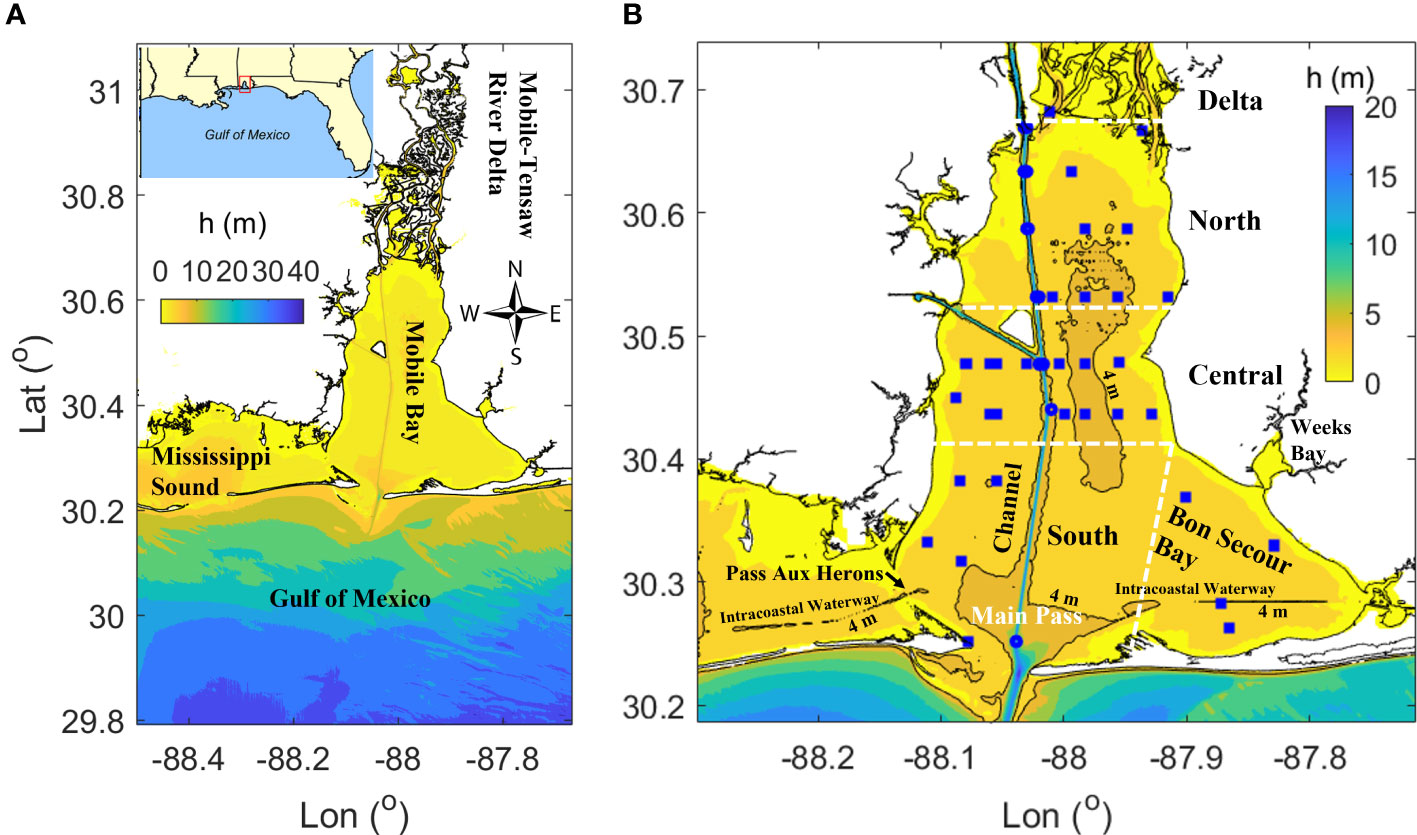
Figure 1 (A) Map of Mobile Bay. (B) Map of subregions in Mobile Bay and observed hypoxic locations for 2019. In (A, B) pseudo-color denote bathymetry. In (B) white dashed lines denote subregion boundaries and the tidal inlet at Main Pass. Narrow black regions down the middle of the bay represent the shipping channels. Narrow channels with 4 m depth in Bon Secour Bay and southwest of Pass Aux Herons are the Gulf Intracoastal Waterway. Blue squares denote all observed hypoxia locations from April to August 2019 (data from Coogan et al., 2021).

Hypoxia occurred both in the deep channel and flat bottom (referred as ‘flank’) in both historical observation (May, 1973; Schroeder and Wiseman, 1988) and recent surveys (e.g., Coogan et al., 2021, Figure 1B). Generally, the large oxygen demand and the strong stratification are principal factors determining oxygen depletion in Mobile Bay bottom water (Turner et al., 1987; Park et al., 2007). Meanwhile, short term destratification events lasting a few days and driven by wind mixing may reoxygenate bottom water, but hypoxic conditions resume within a few hours to days after stratification reestablishes (Park et al., 2007).

2.2 Physical-biogeochemical model

A three-dimensional physical-biogeochemical model of Mobile Bay was developed based on the Regional Ocean Modeling System (ROMS). The model covers the Mobile-Tensaw River Delta, Mobile Bay, part of Mississippi Sound, and nearby coastal region as shown in Figure 2A. A horizontally varying grid was used to resolve the complexity of the system. The grid size is 70 - 90 m in shipping channels and tidal inlets (Figures 2B, C). It gradually increases to 250 - 430 m towards the open boundaries. Vertically, there were 16 layers with near-surface and near-bottom refinement. The wet/dry option was turned on with truncated topography 1.0 m above sea level. The tidal elevation forcing was mapped from the Western North Atlantic, Caribbean and Gulf of Mexico ADCIRC Tidal Databases. Hourly non-tidal water level and currents, temperature, and salinity were applied at the open boundaries using data obtained from the Northern Gulf of Mexico Operational Forecast System (NGOFS, Wei et al., 2014). River discharge was applied at the northern by boundary by summing discharges from three rivers: Alabama River (USGS 02428400), Tombigbee River (USGS 02469761) and Satilpa Creek (USGS 02469800). Meteorological forcing, including 3-hourly solar radiation, precipitation, wind, air temperature, sea surface temperature and humidity, was extracted from the National Centers for Environmental Prediction (NCEP)’s North American Regional Reanalysis (NARR) data. This model configuration allowed for a maximum time step of 3 seconds. Details of the hydrodynamic model setup can be found at the preprint on the Earth and Space Science Open Archive (ESSOAr, https://www.essoar.org/doi/10.1002/essoar.10512128.1).

FIGURE 2

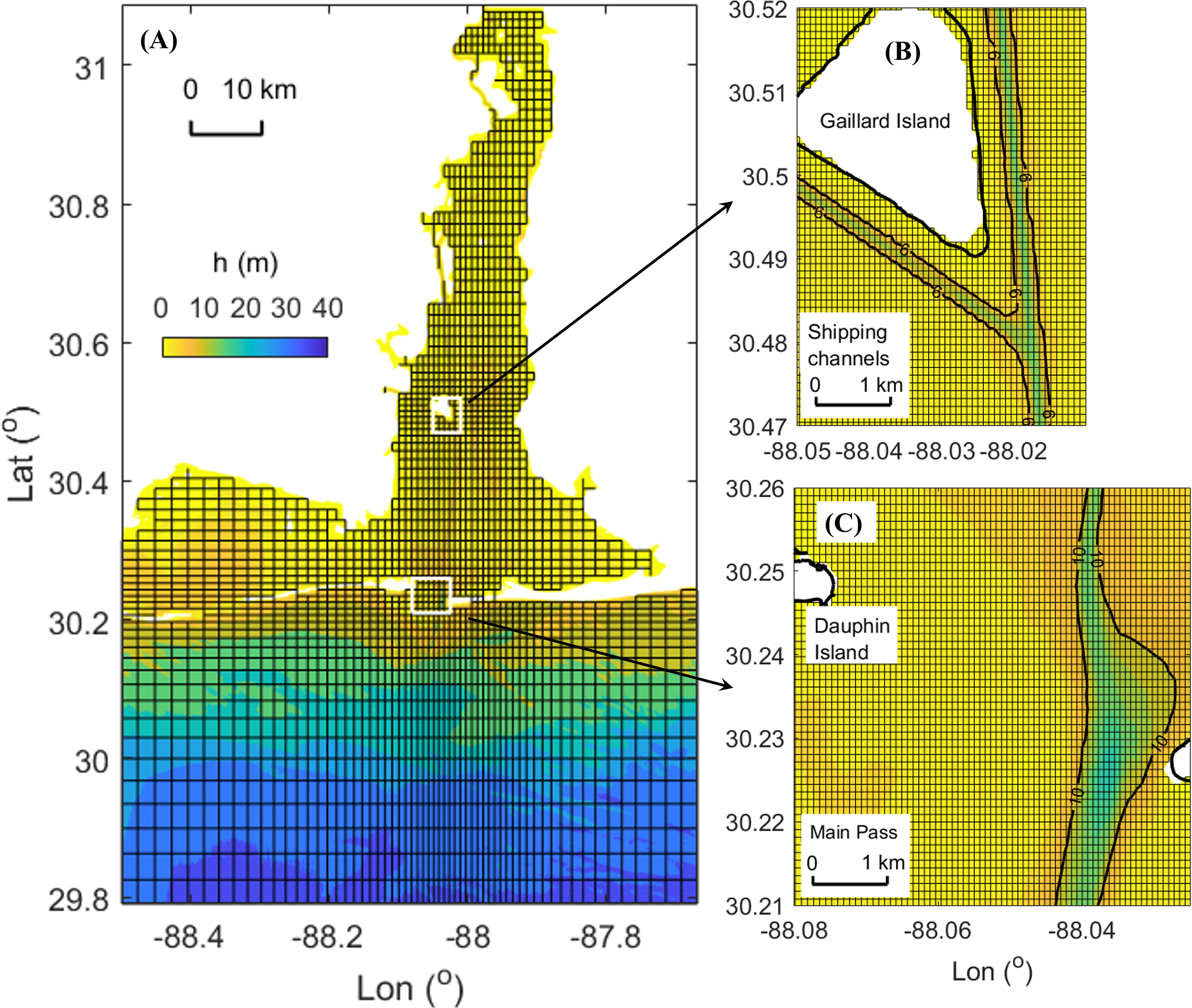
Figure 2 ROMS model domain and grid. (A) Sketch of grid over entire domain. Real resolution is 10-fold finer of the sketch. White boxes denote subregions of panels (B, C). (B) Real grid in shipping channels. (C) Real grid around Main Pass.

Here, we briefly describe the biogeochemical model used, namely, the nitrogen-based model from Fennel et al. (2006; 2008). The model includes state variables for dissolved oxygen (DO); nitrate (NO₃) and ammonium (NH₄) as dissolved inorganic nitrogen; one phytoplankton group (Phy) with chlorophyll (Chl) as a separate state variable; one zooplankton group (Zoo); two types of detritus representing large, large, fast-sinking organic particles (LDetN); and small, slow-sinking organic particles (SDetN). The biogeochemical model also includes dissolved inorganic carbon and alkalinity for representing the CO₂ system, but since those state variables do not affect DO dynamics, they were not analyzed. Primary production (photosynthesis) was the dominant source of DO in the mass balance equation, respiration and nitrification in the water column and bottom sediments were the dominant sink, and the additional source/sink terms included air–sea exchange, advection, and mixing.

Data from the Water Quality Portal (https://www.waterqualitydata.us) for the Alabama River and Tombigbee River was used to calculate the boundary conditions for freshwater river concentrations of NO₃, NH₄, chlorophyll, and organic matter. River phytoplankton concentration in units of mmol N m^-3 was estimated from chlorophyll concentration (mg m^-3) by assuming a phytoplankton mass ratio Chl:C of 1:50 as has been observed in other estuaries (Malone, 1982; Wienke and Cloern, 1987) and further applying the C:N Redfield ratio of 106:16 (Redfield, 1958). River zooplankton was assumed to be 10% of the biomass of phytoplankton (Lindeman, 1942). Data from the water quality portal did not include variables that directly match the model variables SDetN and LDetN. Hence, SDetN and LDetN were calculated as a percent of total Kjeldahl nitrogen (TKN) concentration from the water quality portal as 35% and 65%, respectively, which were the average percentages of dissolved TKN and suspended TKN based on data obtained from the water quality portal. The river oxygen concentration was assumed to be that of the saturation in freshwater.

To focus mainly on biogeochemical processes from the river nutrient dominated area of Mobile Bay and its nearby coastal waters, a zero gradient was applied to all biogeochemical tracers at the open-sea boundaries. Material transport and advection from the distant continental shelf was ignored. Initial conditions for all biogeochemical tracers were estimated using nonlinear regression expressions based on salinity and depth; those expressions were obtained from previous studies of the continental shelf along the northern Gulf of Mexico (2017; Lehrter et al., 2013). Parameter used in the biochemical model, including reaction rates, and sinking velocities are in the Supplementary Material (see Table S1).

2.3 Vertical dissolved oxygen variance

The differential budget equation of VDOV was derived from the Reynolds-averaged budget equation for DO conservation:

$\begin{array}{ll}\frac{\partial DO}{\partial t}+u\frac{\partial DO}{\partial x}+v\frac{\partial DO}{\partial y}+w\frac{\partial DO}{\partial z}=\frac{\partial }{\partial x}\left(K_x\frac{\partial DO}{\partial x}\right)+\frac{\partial }{\partial y}\left(K_y\frac{\partial DO}{\partial y}\right)+\frac{\partial }{\partial z}\left(K_z\frac{\partial DO}{\partial z}\right)+P_p-R& (1)\end{array}$

where x, y, and z represent the horizontal and vertical coordinates, u, v and w are horizontal and vertical components of the three-dimensional velocity vector. P_p is the source term from primary production, while R is the sink term from water column respiration and nitrification. Q_air-sea and Q_SOD are air-sea oxygen exchange and sediment oxygen demand fluxes. K_x, K_y and K_z are eddy diffusivity in horizontal and vertical directions. The boundary conditions of Eq. 1 at surface and bottom are ${K_z\frac{\partial DO}{\partial z}|}_{z=0}=Q_{air-sea}$ and ${K_z\frac{\partial DO}{\partial z}|}_{z=-h}=Q_{SOD}$, where h is depth of water column.

Each variable in Eq. 1 can be decomposed into a depth varying component and a depth averaged component, $va{r}^{\prime }=var-\overline{var}$, where var denotes DO, u, v, w, P_p and R. Substituting the decomposition into Eq.1, integrating over water column, and dropping horizontal diffusion terms, a conservation equation for the depth averaged DO concentration may be derived:

$\begin{array}{ll}\frac{\partial \overline{DO}}{\partial t}+\overline{u}\frac{\partial \overline{DO}}{\partial x}+\overline{v}\frac{\partial \overline{DO}}{\partial y}+\overline{u^{\prime }\frac{\partial D{O}^{\prime }}{\partial x}}+\overline{v^{\prime }\frac{\partial D{O}^{\prime }}{\partial y}}+\overline{w^{\prime }\frac{\partial D{O}^{\prime }}{\partial z}}=\frac{Q_{air-sea}-Q_{SOD}}{h}+\overline{P_p}-\overline{R}& (2)\end{array}$

Taking the difference between Eqs. 1 and 2 results in a differential equation of DO′. Multiplying the differential equation of DO′ and its boundary conditions by 2DO′, the elementary formula of DO′² is derived:

$\begin{array}{ll}\begin{array}{l}\frac{\partial D{O}^{\prime }2}{\partial t}+u\frac{\partial D{O}^{\prime }2}{\partial x}+v\frac{\partial D{O}^{\prime }2}{\partial y}+w\frac{\partial D{O}^{\prime }2}{\partial z}+2D{O}^{\prime }\left(u^{\prime }\overline{\frac{\partial DO}{\partial x}}+2v^{\prime }\overline{\frac{\partial DO}{\partial y}}\right)-2D{O}^{\prime }\left(\overline{u^{\prime }\frac{\partial D{O}^{\prime }}{\partial x}}+\overline{v^{\prime }\frac{\partial D{O}^{\prime }}{\partial y}}+\overline{w^{\prime }\frac{\partial D{O}^{\prime }}{\partial z}}\right)\\ =2D{O}^{\prime }\frac{\partial }{\partial z}\left(K_z\frac{\partial D{O}^{\prime }}{\partial z}\right)-2D{O}^{\prime }\frac{Q_{air-sea}-Q_{SOD}}{h}+2D{O}^{\prime }({P^{\prime }}_p-R^{\prime })\end{array}& (3)\end{array}$

Where the boundary conditions for DO′² are ${K_z\frac{\partial D{O^{\prime }}^2}{\partial z}|}_{z=0}=2D{O^{\prime }}_s{Q}_{air-sea}$ and ${K_z\frac{\partial D{O^{\prime }}^2}{\partial z}|}_{z=-h}=2D{O^{\prime }}_b{Q}_{SOD}$. DO′_s and DO′_b are DO variation at surface and bottom respect to depth averaged value. Note that $2D{O}^{\prime }\frac{\partial }{\partial z}\left(K_z\frac{\partial D{O}^{\prime }}{\partial z}\right)=\frac{\partial }{\partial z}\left(K_z\frac{\partial D{O^{\prime }}^2}{\partial z}\right)-2K_z{\left(\frac{\partial D{O}^{\prime }}{\partial z}\right)}^2$, $\overline{u^{\prime }\frac{\partial D{O}^{\prime }}{\partial x}}+\overline{v^{\prime }\frac{\partial D{O}^{\prime }}{\partial y}}+\overline{w^{\prime }\frac{\partial D{O}^{\prime }}{\partial z}}$ and $\frac{Q_{air-sea}-Q_{SOD}}{h}$ are depth independent, ∫^​DO^′dz=0 , and $\frac{\partial D{O}^{\prime }}{\partial z}=\frac{\partial DO}{\partial z}$. Integrating Eq. 3 over the water column and applying the boundary conditions for DO′² results in the budget for vertical oxygen variance

$\begin{array}{ll}\stackrel{\text{Local tendency}}{{\displaystyle \int }\frac{\partial D{O^{\prime }}^2}{\partial t}dz}=\stackrel{\text{Advection}}{-{\displaystyle \int }\left(u\frac{\partial D{O^{\prime }}^2}{\partial x}+v\frac{\partial D{O^{\prime }}^2}{\partial y}\right)dz}-\stackrel{\text{Physical straining}}{{\displaystyle \int }2D{O}^{\prime }\left(u^{\prime }\overline{\frac{\partial DO}{\partial x}}+v^{\prime }\overline{\frac{\partial DO}{\partial y}}\right)dz}+\stackrel{\text{Air-sea exchange}}{2D{O^{\prime }}_s{Q}_{air-sea}}+\underset{\begin{array}{l}\text{Water column}\\ \text{net metabolism}\end{array}}{{\displaystyle \int }2D{O}^{\prime }({P^{\prime }}_p-R^{\prime })dz}-\underset{\begin{array}{l}\text{Sediment}\\ \text{oxygen demand}\end{array}}{2D{O^{\prime }}_b{Q}_{SOD}}-\underset{\text{Dissipation}}{{\displaystyle \int }2K_z{\left(\frac{\partial DO}{\partial z}\right)}^{2}dz}& (4)\end{array}$

More detailed derivations are given in Section 1 in the Supplementary Material. The term on the left-hand side of Eq. 4 is the local tendency of the VDOV with respect to time. The terms on the right-hand side are the source and sink terms for the local changes in the VDOV. The general advection term in the oxygen budget is naturally decomposed into two processes in the vertical oxygen variance budget, the horizontal movement of vertical oxygen variance (i.e., the advection term) and titling of vertical oxygen profile by horizontal oxygen transport (i.e., physical straining). The horizontal advection is either transport of VDOV from other locations to a local point (positive/convergence) or exporting VDOV from a local point (negative/divergence). The physical straining is the vertical shear in the horizontal velocity acting in conjunction with the horizontal gradient in the DO with positive values enhancing the vertical gradient and negative values indicating a homogenization of the DO structure in the water column. The air-sea exchange (third) term is the contribution of a flux resulting from the deviation between the oxygen concentration of the surface water and its saturation level at the air-sea interface to total VDOV. The fourth and fifth term are the changes resulting from the net metabolism effects in water column and at the bottom. The net metabolism in the water column can either be a source (positive) or sink (negative) term for VDOV depending on the magnitudes of production and respiration, while the bottom oxygen demand is always a source (positive) term for VDOV. The last term in Eq.4 is the vertical dissipation due to vertical turbulent mixing, which always reduces VDOV. The dominant processes in a hypoxia event may be identified by examining the magnitude of each of these terms. MATLAB code with implementation of this approach can be found in https://github.com/OyBcSt/Vertical-DO-variance_MATLAB.

3 Results

3.1 Model validation

Three metrics were used to assess model performance:

$\begin{array}{ll}\begin{array}{cc}\text{mean error},ME=\frac{1}{N}\sum _{i=1}^N(M-O);& (2a)\\ \text{mean absolute error},MAE =\frac{1}{N}\sum _{i=1}^N\left|M-O\right|;& (2b)\\ \text{and model skill},skill = 1-\frac{\sum {\left|M-O\right|}^2}{\sum {(\left|M-\tilde{O}\right|+\left|O-\tilde{O}\right|)}^2}.& (2c)\end{array}& (5)\end{array}$

Where O and M are observed and modeled data, respectively (Wilmott, 1981). The overbar indicates a temporal average over the number of observations (N). The magnitudes of ME and MAE indicate the average bias and deviation while Skill acts as a global index of overall agreement between model and observation. Skill = 1 means the model matches the observations perfectly, while Skill = 0 means there is absolutely no overlap between model and observation.

The modeled temperature and salinity at 0.5 m above bottom were validated by hourly field data at 5 mooring stations in Mobile Bay and 1mooring station in Mississippi Sound from Alabama’s Real-Time Coastal Observation System (ARCOS, https://arcos.disl.org/). Model skill parameters are listed as follows: for temperature, ME = 0.37 ~ 1.62 °C, MAE = 1.33 ~ 1.79 °C and Skill = 0.97 ~ 0.98. For salinity, ME = 0.06 ~ 5.13 psu, MAE = 0.73 ~ 8.09 psu and Skill = 0.43 ~ 0.90. For stratification measured by depth averaged vertical salinity variance, ME = -7.56 psu², MAE = 11.41 psu² and Skill = 0.76, see Table S2 in the complimentary material. Figures of the hydrophilic validation can be found in the preprint on ESSOAr (https://www.essoar.org/doi/10.1002/essoar.10512128.1).

The hourly time-series of modeled DO at 0.5 m above the bottom compared favorably with observational time-series at 3 ARCOS mooring stations across the bay, all of which had a mean error less than 0.6 mg L^-1 and skill above 0.40 (Figure 3). The model captured the hypoxia events in late April and early May, as shown by the model-observation comparison at Bon Secour (BS) station (Figure 3C). During a hypoxia event the bottom DO has strong horizontal gradients as indicated by the model results at a virtual station (BS’), 4.9 km northwest of the real BS station, which captured almost all the observed hypoxia events in Bon Secour Bay. The oxygen dynamics in Bon Secour Bay were likely controlled by nutrient loading from upstream rivers and the nearby sub-estuary Weeks Bay. Therefore, the tidal variation of DO at BS station was weak in comparison to the modeled DO at Main Pass (DI) and the northern end (MP) that had strong tidal variation.

FIGURE 3

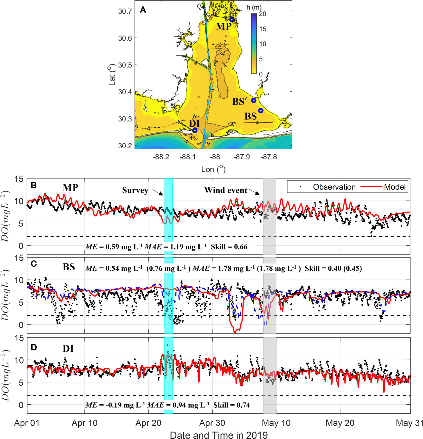
Figure 3 Time-series of hourly dissolved oxygen (DO) concentration at 0.5 m above bottom during April-May from ARCOS observation and model results. (A) Map of ARCOS stations at Meaher Park (MP), Dauphin Island (DI), and Bon Secour (BS and BS’). Next are DO concentration time-series for each of those stations: (B) MP (C) BS and BS’ (blue dashed line). BS’ is a virtual station 4.9 km northwest of real observation station. (D) DI. Black dashed lines denote hypoxia threshold of 2 mg L^-1. Box in cyan denotes bay-wide survey during April 22-23. Box in grey denotes the southeast wind event during May 8-9.

A bay wide CTD profiling survey of 80 stations during April 22-23 (Coogan et al., 2021) was also used to verify the model’s ability to match observed spatial patterns (Figure 4). Overall, the model performed well with mean errors between model outputs and survey data for surface and bottom DO differences being -0.86 mg L^-1 and -0.30 mg L^-1, respectively. The corresponding skill values were 0.64 and 0.68 indicating that the model favorably captured oxygen dynamics in the bay allowing it to reproduce the spatial heterogeneity in oxygen distributions. Relatively high surface DO (> 10 mg L^-1) occurred in the southwestern bay and was spatially uniform (8.5 ~ 9.5 mg L^-1) in Bon Secour Bay (Figures 4A.1, A.2). Bottom DO was relatively lower (< 7 mg L^-1) in Bon Secour Bay (Figures 4B.1, B.2). Note that the model underestimated DO at both surface and bottom by 2 mg L^-1 in the northern-most part of the bay. These extreme deviations led to a system-wide mean absolute error of 1.32 ~ 1.33 mg L^-1. In other regions of the bay, deviations were smaller, but there was a bias up to + 2 mg L^-1 in bottom water across some near shoal areas including the eastern central region and in Bon Secour Bay.

FIGURE 4

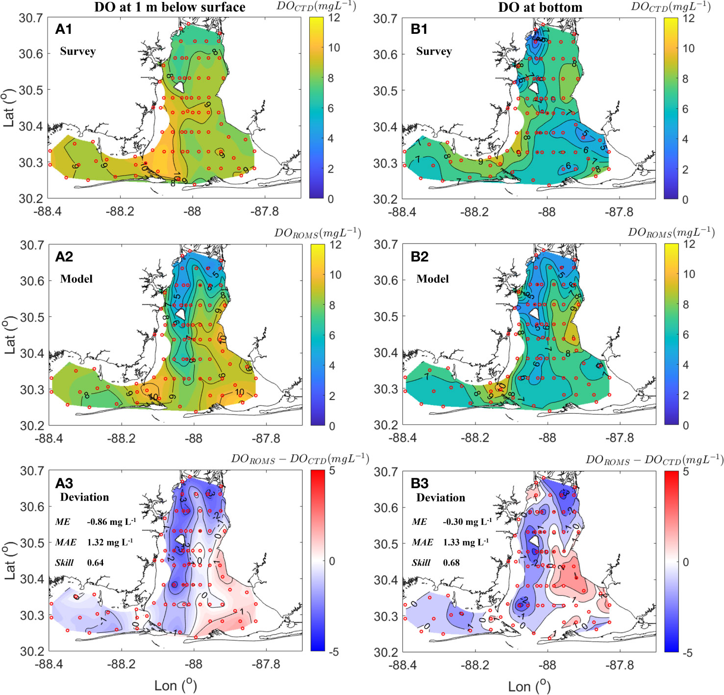
Figure 4 Spatial patterns of dissolved oxygen (DO) concentration during April 22-23. Figure includes (A.1) DO at 1 m below the surface from CTD profiling, (A.2) modeled DO at 1 m below the surface, (A.3) model deviation at 1 m below the surface (modeled DO from ROMS – observed DO from CTD) shown with ME, MAE, and Skill, (B.1) DO at bottom from CTD profiling, (B.2) modeled DO at the bottom, and (B.3) bottom model deviation (modeled DO from ROMS – observed DO from CTD shown with ME, MAE, and Skill. Red circles in all panels denote CTD stations.

The modelled spatial patterns of chlorophyll (Chl) concentration also compared well with the field samples collected at 15 water sample stations during April 22-23 (Figure 5). The surface Chl concentration generally increased from 5 mg m^-3 to 30 mg m^-3 from the delta toward tidal inlets (Figure 5A.1). Patches with Chl above 20 mg m^-3 in the upper 1.5 m water column were located at southwest and southeast bay (i.e., Bon scour Bay), where the higher near surface DO was above 9 mg L^-1 (Figure 4A.1). The model reproduced the general patterns especially those high Chl patches resulting in a skill score of 0.84 (Figures 5A.2, B.2). Major deviations occurred in the northern bay where the model underestimated Chl by around 5 mg m^-3.

FIGURE 5

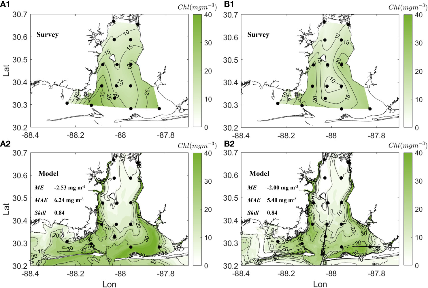
Figure 5 Spatial patterns of chlorophyll (Chl) concentration during April 22-23. Figure includes (A.1) Chl at surface, (A.2) modeled surface Chl with ME, MAE, and Skill, (B.1) Chl at 1.5 m below the surface, (B.2) modeled Chl at 1.5 m below the surface with ME, MAE, and Skill. Black circles in all panels denote CTD stations.

Regions with bias up to 2 mg L^-1 in DO overlapped with regions where modelled phytoplankton had large bias compared to Chl observations (Figures 4A.3, B.3, 5A.1, B.2). The potential time lag in the evolution of these bloom patches or sinking of detritus between the model and field data might result in the bias in oxygen. Other limitations of the present model as well as challenges in modeling the Mobile Bay system are discussed in section 4.

3.2 Linkage between bottom DO and vertical dissolved oxygen variance

To assess the usefulness of VDOV in assessing the DO dynamics, a relationship with bottom DO concentration needs to be established. The large vertical differences between the surface and bottom result in a large VDOV. Thus, it might be expected that the lower the bottom oxygen concentration is, the larger the VDOV should be, resulting in a negative correlation. This expectation was verified using an exponential regression between depth averaged VDOV ($\overline{D{O}^{\prime }2}$) and bottom DO concentration (DO_b) collected from April to September 2019. An R² of 0.94 for 465 profiles collected at locations outside of the shipping channel (denoted as ‘flank’ stations in Figure 6) and an R² of 0.58 for 80 profiles collected in the shipping channel (Figure 6). Based on the regression analysis, hypoxia (< 2 mg L^-1) is typically observed when $\overline{D{O}^{\prime }2}$ is 3.86 mg² L^-2 over the flank and 2.14 mg² L^-2 in the shipping channel. The nonlinear relation between $\overline{D{O}^{\prime }2}$ and DO_b highlighted that a decline in bottom oxygen could exponentially amplify the variance in DO profile. Verification of VDOV as a proxy for hypoxia occurrence confirms that the approach shown in Eq. 4 may be applied to study the impact of wind on hypoxia in Mobile Bay.

FIGURE 6

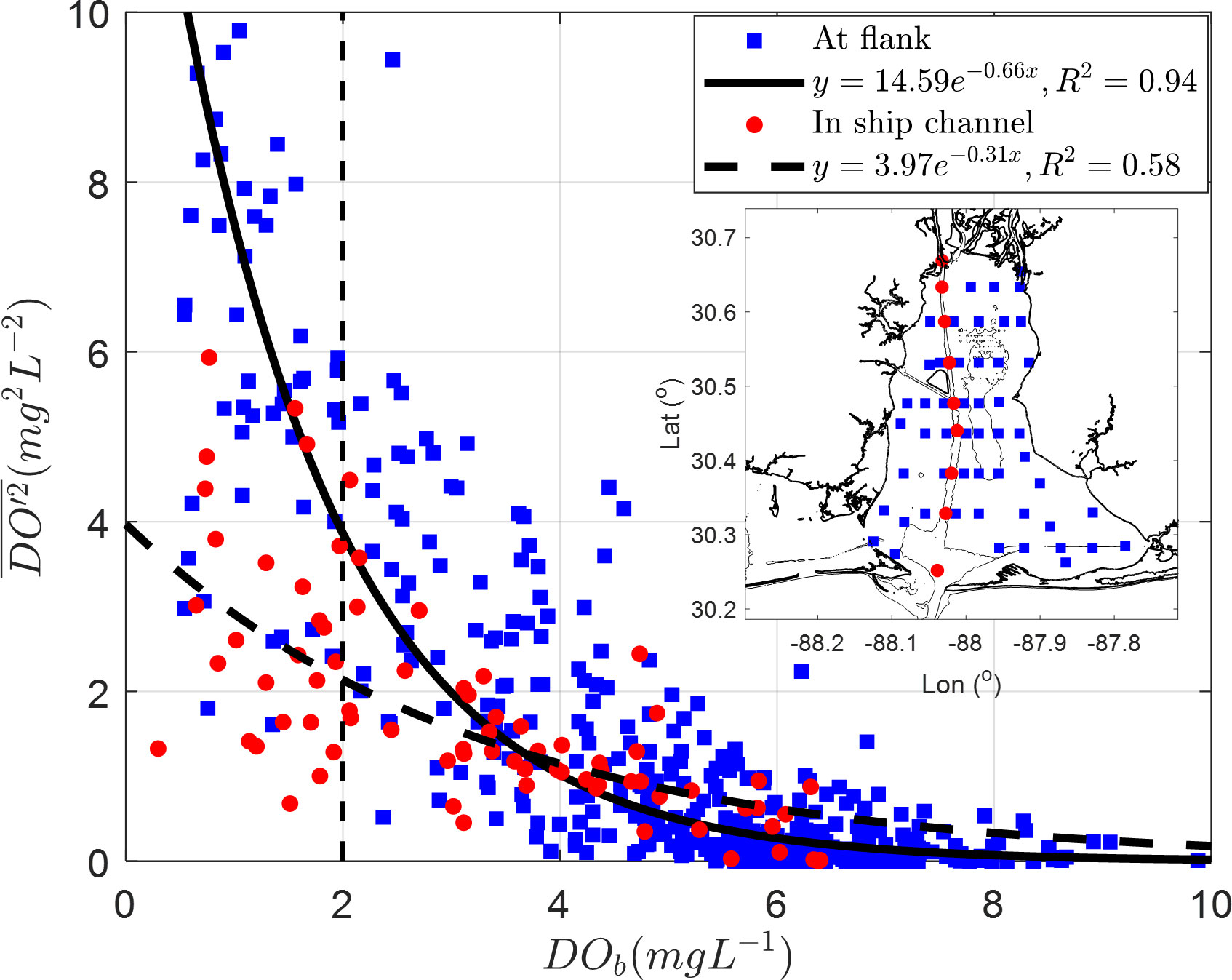
Figure 6 Relationship between depth averaged VDOV, $\overline{D{O^{\prime }}^2}$ and DO_b was computed from DO concentration profiles collected in Mobile Bay from April to August, from 0.6 m below surface to the bottom (Coogan et al., 2021). The subpanel denotes map of DO profile stations. Blue squares are from 465 profiles collected in areas outside of the shipping channel (i.e., flanks), and the solid black line is an exponential fit to these data. Red circles are from 80 profiles collected in the shipping channel, and the black dashed line is their corresponding fit.

3.3 Hypoxia event in early summer

Field survey data and time-series station data both indicate that low oxygen developed in late April and persisted through early May. The development and destruction of this event was tracked against VDOV and its associated budget terms.

In the model, a hypoxic event occurred in late spring. The volume averaged VDOV over the bay area (Figure 7A) tracked the processes driving the hypoxia event, starting from pre-cursor phytoplankton blooms, and ending by wind-driven destruction. Starting April 24, the hypoxia area (A_h) increased linearly until May 4 when it reached a peak value of 160 km² (Figure 7D). The hypoxic area then rapidly dissipated, disappearing in 6 days. During hypoxia development, volume averaged VDOV, DO′², exhibited short term fluctuations but had a globally increasing trend (Figure 7D). DO′² reached to its first peak (2.44 mg² L^-2) together with the peak phytoplankton bloom around April 29 (Chl = 28.44 mg m^-3, Figure 7C). During this period, both the primary production and sediment oxygen demand (SOD) produced top-to-bottom differences in oxygen profiles (Figure 7E).

FIGURE 7

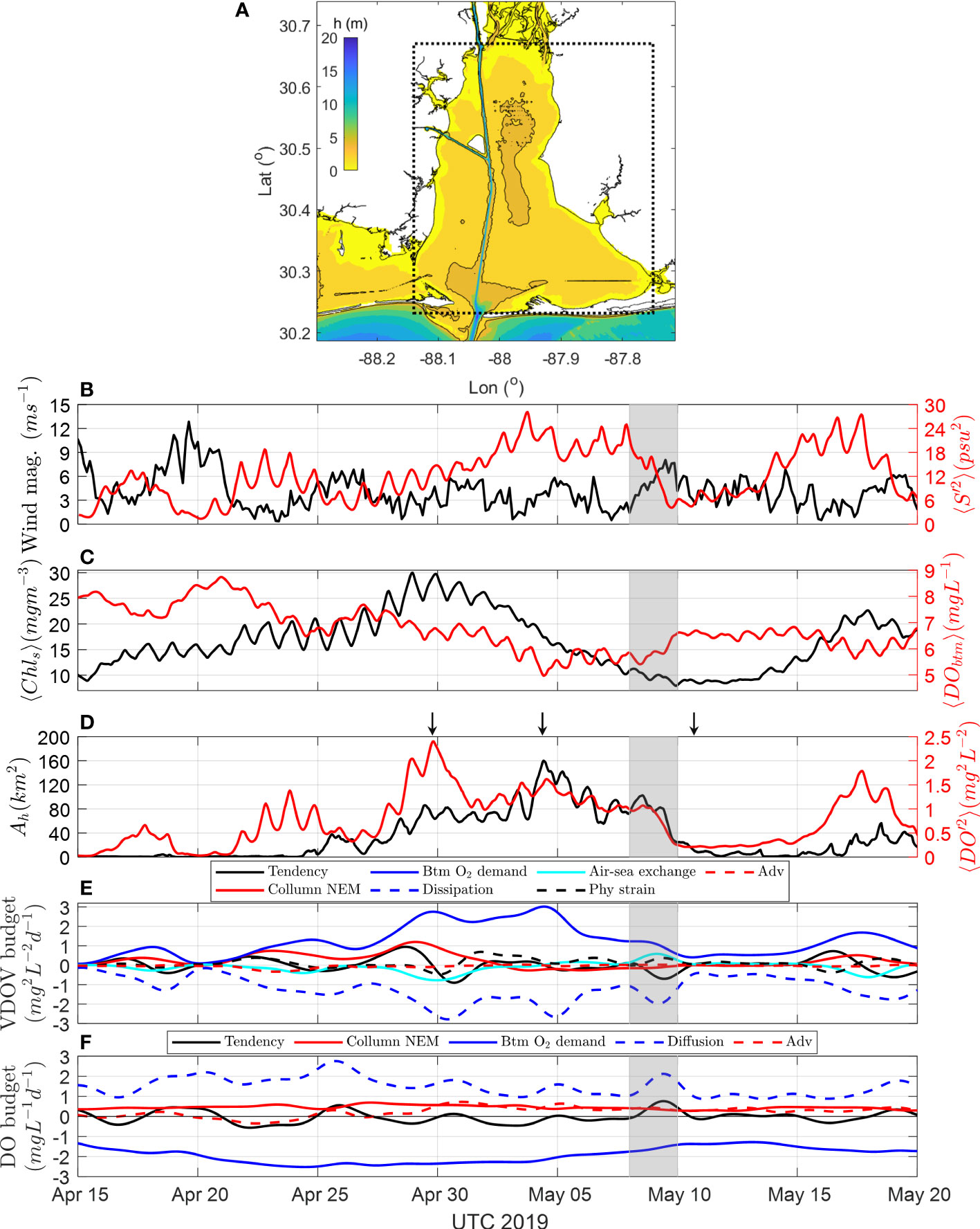
Figure 7 Evolution of wind, stratification, phytoplankton bloom and hypoxia. (A) Region for taking spatial average. (B) 3-hour averaged raw wind speed in the center of Mobile Bay from NARR and volume averaged vertical salinity variance (S′²). (C) Spatially averaged surface chlorophyll concentration (Chl) and bottom DO (DO_b). (D) Hypoxia area A_h, and volume averaged DO′². Arrows denote the time points of Figure 8. (E) Volume averaged VDOV budget terms. Positive terms denote mechanisms creating oxygen variance, while negative terms denote mechanisms destructing oxygen variance. (F) Volume averaged DO budget terms in the lower 1/3 water column. Positive terms denote mechanisms increase DO in lower water column, and negative terms denote mechanisms decreasing DO in lower water column. A low-pass 48-hr Lanczos filter was applied to both VDOV and DO budget terms shown in panels (E, F). Grey boxes in all panels denote a southeast wind event during May 8-10.

After the phytoplankton bloom, DO′² reached its second peak (1.62 mg² L^-2, Figure 7D) at the minima of the spatially averaged bottom DO around May 4 (DO_b = 4.40 mg L^-1, Figure 7C). The interval (~ 5 days) between the first and second peaks in DO′² exactly reveals the time lag between the pre-cursor phytoplankton bloom and the following hypoxia event. Following this peak, DO′² and A_h were synchronous until the end of the hypoxia event (Figure 7D), since the sediment oxygen demand (SOD) was the only significant process contributing to the oxygen variance (Figure 7E).

During this hypoxia event, dissipation was the dominant term balancing variance production from water column metabolism and sediment oxygen demand (SOD). Peak values of dissipation matched wind and mixing events over the study period (Figures 7B, E). For example, the wind event (~ 6 m s^-1) around May 5 reduced bay wide salinity variance by 53.4% (Figure 7B) and induced dissipation (2.7 mg² L^-2 d^-1) that nearly balanced SOD, resulting in a decline in the hypoxia area of 50 km². A subsequent wind event (~ 8 m s^-1, May 9, grey box in Figure 7) almost mixed the entire system and resulted in a dissipation twice that of SOD, reducing the remaining hypoxia area by 76% (Figures 7D, E). From the VDOV budget analysis of this hypoxia event, wind-induced dissipation clearly dominates the reoxygenation of the water column.

Identical patterns were demonstrated by a DO budget analysis for the bottom 1/3 of the water column (Figure 7F). Through April 20 to May 5, a stable sediment oxygen demand of 2.0 ~ 2.5 mg L^-1 d^-1 promoted a negative tendency in the DO budget of – 0.4 ~ – 0.6 mg L^-1 d^-1 and continuous reduced bottom DO. Short term wind mixing events stimulated vertical diffusion exceeding sediment oxygen demand and reoxygenated the bottom water (Figures 7B, C, E, F). However, the phytoplankton bloom was not explicitly indicated since surface processes were not included in the subsurface DO budget analysis.

To verify contributions of the pre-cursor phytoplankton bloom to the development of hypoxia, the spatial patterns of surface Chl concentration before, during and after the hypoxia event were further examined. At the peak phytoplankton bloom on April 29, surface Chl was above 30 mg m^-3 over most of the bay with peak values above 42 mg m^-3 in south bay and Bon Secour Bay (Figure 8A). Five days later, surface Chl in lower bay dropped to 10 mg m^-3, where detritus from the phytoplankton bloom stimulated abundant oxygen demand pushing the hypoxic area to a maximum (Figure 8B). After peak hypoxia, surface Chl in the lower bay further dropped to below 1 mg m^-3 till the end of hypoxia event (Figure 8C). The evolution of Chl was consistent with the evolution of hypoxia as well as VDOV budget analysis. Furthermore, the spatial pattern of Chl also indicated that portions of the southern region of the bay and Bon Secour Bay would be specific locations associated with hypoxia during this event. Therefore, contributions of wind to hypoxia destruction over these regions will be further investigated in the next section.

FIGURE 8

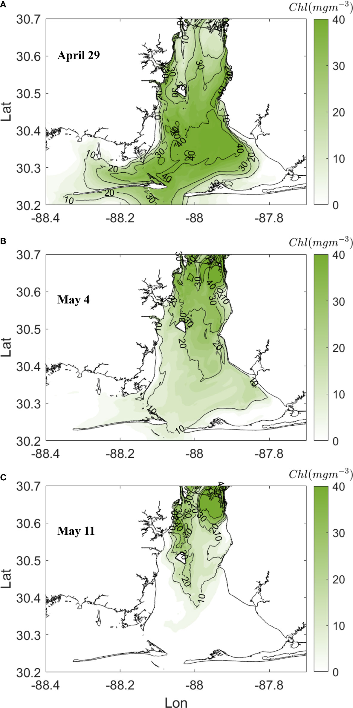
Figure 8 Spatial patterns of surface chlorophyll (Chl) concentration before (A), during (B) and after (C) the hypoxia event in early May 2019.

3.4 Wind impact on hypoxia

Previous analysis highlighted rapid destruction of hypoxia during a wind event around May 9. The wind driven processes including dissipation and advection from wind driven circulation on reoxygenation are investigated based on detailed VDOV budget analysis.

3.4.1 Hypoxia destruction

Spatial patterns in bottom DO concentration and VDOV budget terms show the importance of local changes in the dominant processes during the southeast wind event (May 8 - 10) that dissipated the hypoxia. Prior to the onset of the wind event (1.86 m s^-1, 1800 May 7, Figure 9D), the major hypoxic zone was in Bon Secour Bay (64.65 km²) and a minor zone was in southwestern part of the bay (9.83 km²) in the shape of a narrow strip. During the initial onset of the wind event, approximately 18 hours after the wind transitioned to the southeasterly direction (4.71 m s^-1, 1200 May 8, Figure 9A), the spatial patterns of hypoxia remained persistent with the hypoxic zones increasing to 74.33 km² in Bon Secour and 27.62 km² in southwestern bay, respectively (Figure 9C). Noticeable declines of hypoxia were much more apparent when peak wind-speed reached 8.05 m s^-1 (May 9, Figure 9D). The western tip of the hypoxic zone in Bon Secour Bay disappeared, while the remaining zone (23.9 km²) shifted ~3 - 4 km downstream. Similarly, the hypoxic area in the southwestern bay shrunk to 19.28 km². After maintaining peak wind-speeds for ~9 hours, wind conditions transitioned into a period of relative quiescence (Figure 9A). The hypoxic area decreased by 45.35 km² over the 9-hour period, accounting for 58% of the total decline over the entire wind event (Figures 9C–E).

FIGURE 9

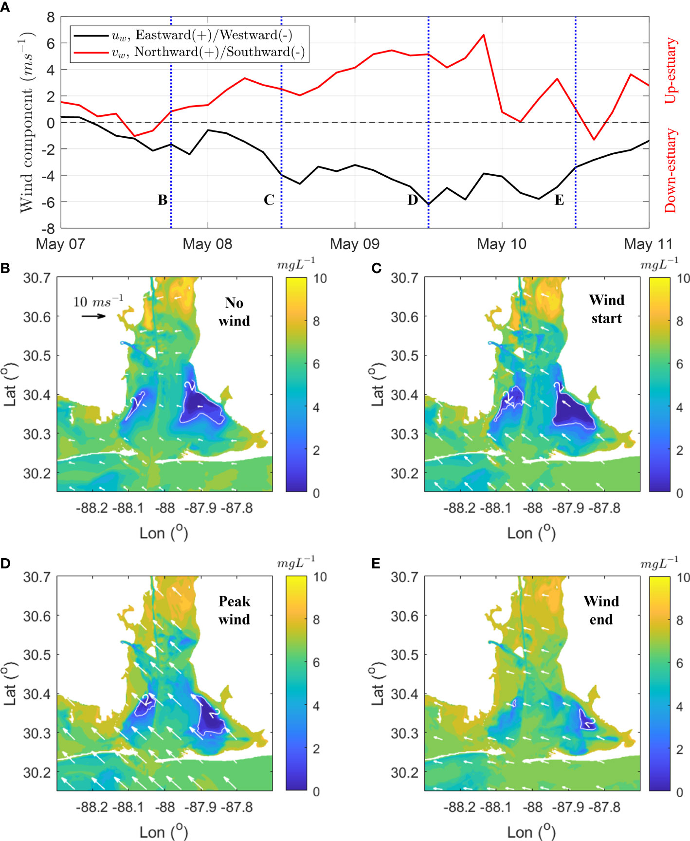
Figure 9 Evolution of bottom DO during a southeast wind event on May 8 – 10. (A) solid lines are 3-hourly averaged raw wind-speed in the center of Mobile Bay (data from NARR) and blue dashed lines denote times corresponding to different phases of the wind event shown (B–E). (B–E) Snapshots of the evolution of bottom DO concentration over the southeast wind event: (B) event initiation, (C) event onset, (D) event peak, and (E) event end. White arrows show magnitude and direction of wind, and the solid white contour lines show the boundaries of the hypoxic zones.

3.4.2 VDOV budget

The spatial patterns in VDOV budget terms highlight the local contributions of each process during hypoxia destruction. As expected from the decrease in the hypoxic area over the course of the southeast wind event (Figure 10), there was a negative tendency of 3 - 6 mg² L^-2 d^-1 (Figure 10A). Maximum tendencies of up to 8.5 mg² L^-2 d^-1 occurred in Bon Secour Bay, indicating that a southeast wind blowing for 1 day was able to remove hypoxia at these locations. Consistent with the temporal trends shown in Figure 10C, the vertical dissipation of 5 - 10 mg² L^-2 d^-1 was roughly mirroring the patterns of tendency in Bon Secour Bay as well as southwestern part of Mobile Bay (Figure 10B).

FIGURE 10

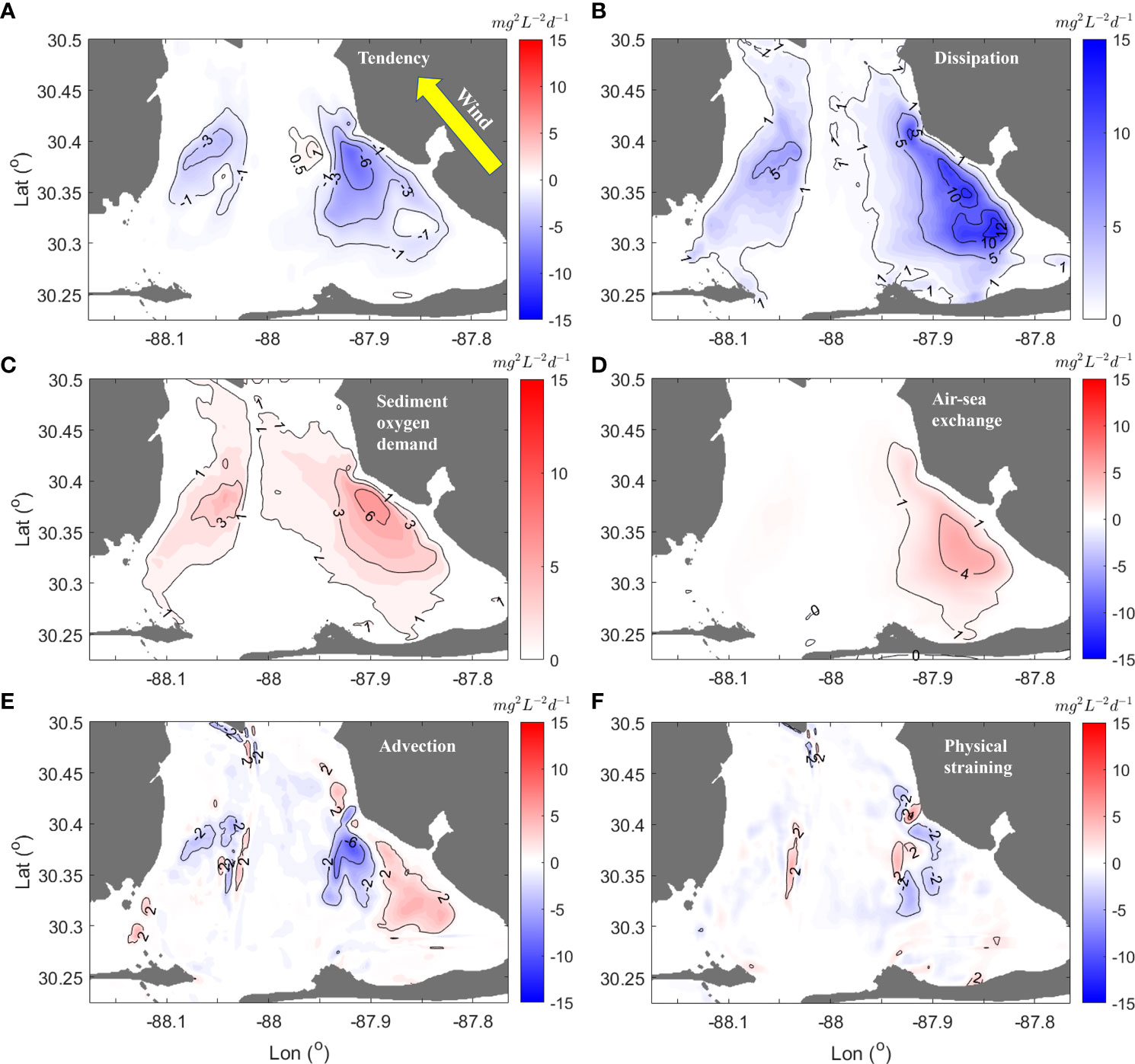
Figure 10 Terms in the vertical dissolved oxygen variance (VDOV) budget (mg² L^-2 d^-1) during a southeast wind event. Panel (A–F) are spatial patterns of corresponding terms of VODV budget equation (Eq. 4). Red color denotes positive tendency, advection, and physical straining (i.e., increasing VDOV); blue color denotes negative tendency, advection, straining and dissipation (i.e., decreasing VDOV). All terms were temporally and vertically averaged over a 36-hour period between May 8 - 10.

The spatial patterns of sediment oxygen demand (3 - 6 mg² L^-2 d^-1, Figure 10C) roughly mapped with the bay-wide hypoxic zones. Another source term for VDOV was air-sea exchange (4 mg² L^-2 d^-1) in a portion of Bon Secour Bay. Physically, this source term indicated that oxygen injection from the atmosphere to the water column maintained the bottom-to-surface difference in DO profiles during hypoxia destruction.

In Bon Secour Bay, the adjacent negative (-3 ~ -6 mg² L^-2 d^-1) and positive (2 mg² L^-2 d^-1) zones of the advection term suggested a directional transport of hypoxic water from central and south zones to the Bon Secour Bay zone (Figure 10E). This transport also tended to increase bottom DO, highlighted by the negative physical straining (-2 mg² L^-2 d^-1, Figure 10F), but its magnitude was far less than the dissipation term. Wind-induced dissipation was the dominant reoxygenation process in bay-wide destruction of hypoxia, while oxygen transport contributed to the local patterns of hypoxia. The next section will discuss the link between estuary circulation and oxygen transport.

3.4.3 Wind induced advection and dissipation

During the southeast wind event, subtidal circulation deviated from typical estuarine-exchange flow patterns where the horizontal density gradient drives surface outflow and bottom inflow. The southeast wind-driven surface current generally flowed up-estuary in the direction of the wind (Figure 11A), while the return flow in the bottom was southeastward opposite the wind direction. This wind driven subtidal flow patterns was opposite typical estuarine subtidal flow.

FIGURE 11

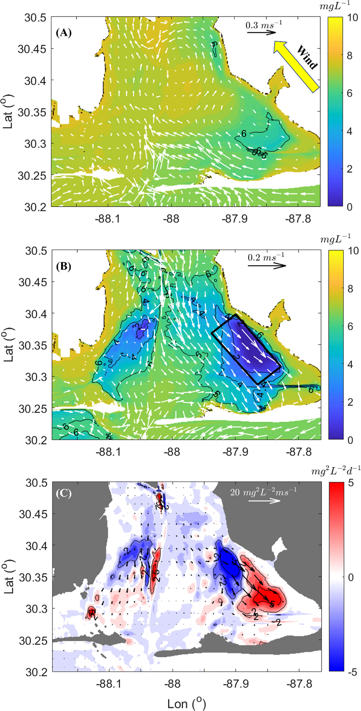
Figure 11 Low pass filtered current (vectors) and oxygen concentration (contour lines) during peak southeast wind speed (May 9) at surface (A) and bottom (B). Thick black box denotes spatial averaging zone of Figure 9. (C) Low pass filtered depth averaged VDOV flux $\overline{uD{O^{\prime }}^2}$ and $\overline{vD{O^{\prime }}^2}$ (vectors) and advection term in VDOV budget (coloration). Red denotes convergence (incoming) of VDOV flux, blue color divergence (outgoing) of VDOV flux.

In addition, there were significant spatial differences in the bottom currents. Intensified down-estuary current (~ 0.1 m s^-1) was confined to Bon Secour Bay. The current was less than 0.05 m s^-1 in the southwestern part of the bay (Figure 11B). This is consistent with intensified downstream advection of hypoxic bottom water and with the high VDOV flux of ~13 mg² L^-2 m s^-1 [vector ($\overline{uD{O}^{\prime }2}$, $\overline{vD{O}^{\prime }2}$), Figure 11C]. Intensified bottom current also enhanced vertical mixing and corresponded to a high dissipation zone of vertical oxygen variance in Bon Secour Bay (Figure 8B). Wind-induced bottom flow moved the hypoxic zone further downstream to regions having higher dissipation.

3.5 Generalizing advection and diffusion in controlling DO dynamics

To generalize these findings, the contributions of advection and vertical diffusion to hypoxia destruction can be scaled by as $\frac{K_{z}L}{u_s{h}_{sp}^2}$ (see detailed derivation at Section 2 in the Supplementary Material). In the scaling number, u_s streamwise bottom flow (including both tidal and subtidal components, 0.13 m/s in this work); L is the length scale of the hypoxic zone in the direction of streamwise flow (~ 11.4 km in this work); h_sp is sub-pycnocline layer thickness, which can be scaled as the bottom boundary layer thickness h_bl; K_z is the eddy diffusivity at the pycnocline (~ 10^-5 m² s^-1 in this work). Physically, this ratio can be understood as a comparison of timescales, where $T_{adv}~\frac{L}{u_s}$ is the timescale required for advection to remove hypoxia from the system and $T_{diff}~\frac{h_{sp}^2}{K_z}$ is the timescale required for turbulent diffusion to remove hypoxia. Therefore, $\frac{T_{adv}}{T_{diff}}~\frac{K_{z}L}{u_s{h}_{sp}^2}$ should be considered as the time ratio between advection and turbulent diffusion in ameliorating hypoxia.

Hypoxia is not simply a physical process, and biogeochemical processes need to be considered. Given the dominance of the sediment oxygen demand and turbulent dissipation in Mobile Bay, a balance between sediment oxygen demand and turbulent mixing can be considered. At steady state, the 2D transport equation of DO reduces to $K_z\frac{{\partial }^{2}DO}{\partial z^2}=0$ with a bottom boundary condition of $K_z\frac{\partial DO}{\partial z}=Q_{SOD}$ and DO = DO_s at pycnocline. Bottom DO concentration is $D{O}_b=D{O}_s-h_{sp}\frac{Q_{SOD}}{K_z}$. By letting DO_b = 0, a demand-diffusion flux ratio (R_dd) may be obtained where $R_{dd}=\frac{Q_{SOD}}{K_{z}D{O}_s/h_{sp}}$ and scales the ratio of sediment oxygen demand to vertical turbulent diffusion flux through the pycnocline. Generally, R_dd > 1 indicates that oxygen demand exceeds vertical diffusion and a decreasing trend in bottom DO would be expected, while R_dd > 1 indicates vertical diffusion overcomes bottom demand and an increasing trend in bottom DO would be expected.

Examining the behavior of these non-dimensional numbers during this southeast wind event demonstrates their usefulness. For the timescale ratio, the advection timescale was larger than turbulent diffusion, i.e., $1<\frac{T_{adv}}{T_{diff}}<1.5$ (blue solid line with circles, Figure 12B), indicating that advection had less of a contribution than turbulent diffusion as the hypoxia decayed. This is consistent with the VDOV budget analysis. With regards to the demand-diffusion flux ratio, values of R_dd > 1 during the initial, weak wind conditions (< 5 m s^-1) corresponded to a reduction in DO (blue dashed line with hexagons, Figure 12B). When wind speed exceeded 5 m s^-1, salinity variance (S′²) dropped below 10 psu² (Figure 12A) and R_dd was below 1, suggesting that wind-induced turbulence and mixing reduces stratification and ‘pumped’ oxygen to bottom water at a rate in excess of bottom demand. Again, the dynamics captured by R_dd follow the results from the analysis of model outputs.

FIGURE 12

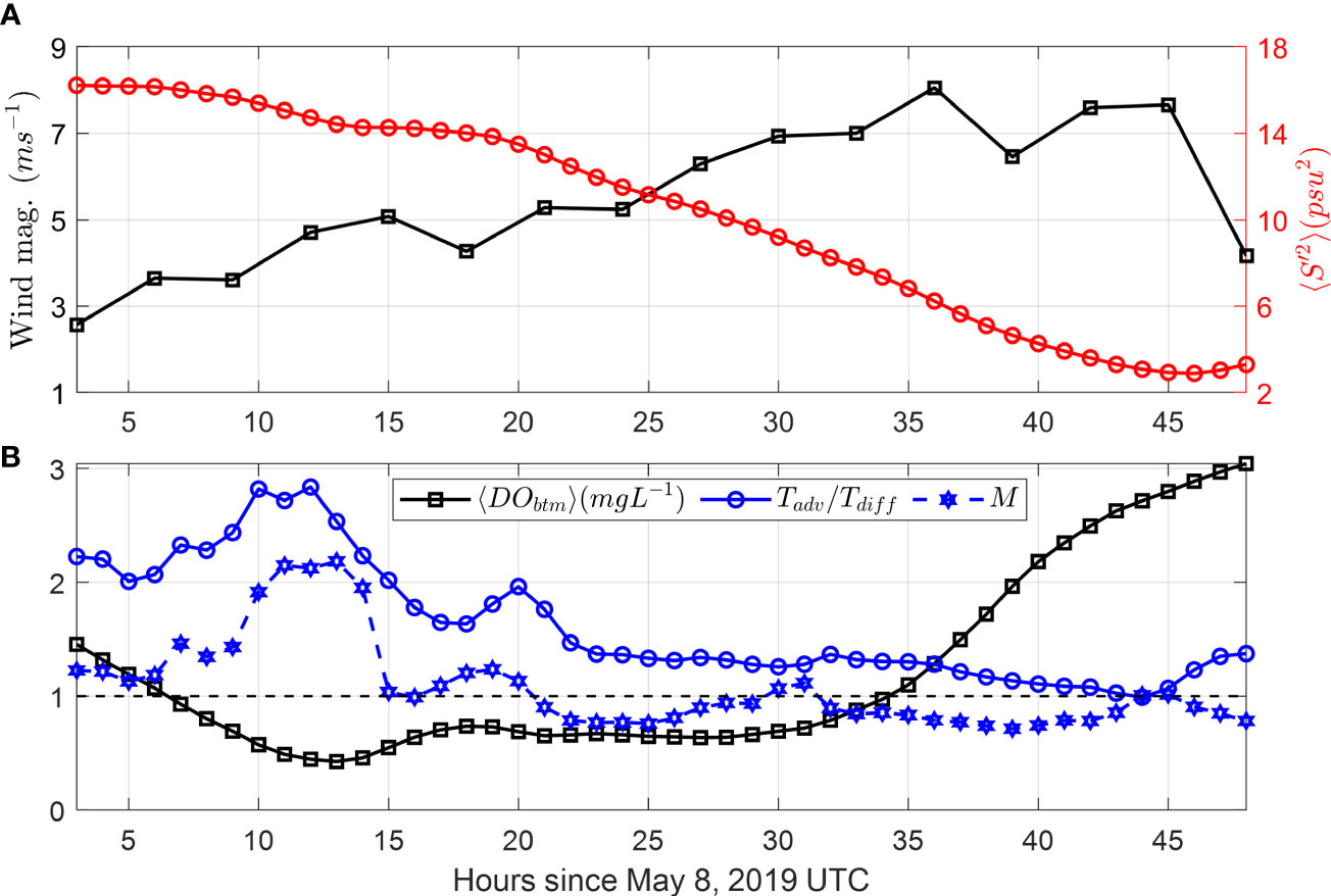
Figure 12 (A) Time series of magnitude wind speed and spatially averaged salinity variance 〈S′²〉 under southeast wind. (B) Time series of bottom DO 〈DO_b〉, advection-diffusion scaling $\frac{T_{adv}}{T_{diff}}~\frac{K_{z}L}{u_s{hsp}^2}$, and demand-diffusion flux ratio $R_{dd}=\frac{Q_{SOD}}{K_{z}D{O}_s/h_{sp}}$. In panel (B), dashed black line denotes $\frac{T_{adv}}{T_{diff}}$ = 1 and R_dd = 1. In panels (A, B), spatial averaging zone is shown by the thick black box in Figure 11B.

4 Discussion

The sub-pycnocline DO budget analysis approach is appropriate in systems like the northern Gulf of Mexico (Yu et al., 2015; Xomchuk et al., 2021) and Chesapeake Bay (Scully, 2010b), where the depth of the pycnocline is fairly stable through the hypoxia season. In a system like Mobile Bay the pycnocline depth is very dynamic and the pycnocline is frequently destroyed by wind mixing. Thus, even though we know exactly where the pycnocline is based on the model outputs, it is not straightforward to do a budget analysis based on a very dynamic pycnocline in systems like Mobile Bay. Thus, the vertical dissolved oxygen variance (VDOV) method was developed for entire water column regardless of depth of the pycnocline. Despite considering the entire water column, the method can still quantitatively split the physical and biogeochemical factors controlling dissolved oxygen dynamics and naturally decomposes advection contributions into two processes (horizontal advection versus physical straining) that are not well captured in a generic sub-pycnocline DO oxygen budget analysis. Thus, using the VDOV, the importance of the horizontal movement of vertical oxygen variance (i.e., advection of oxygen variance) and titling of vertical oxygen profile by horizontal oxygen transport (i.e., physical straining) can be easily assessed. Furthermore, unlike traditional subtidal bottom DO budget analysis, contributions of the surface processes such as primary production and air-sea flux exchange to oxygen dynamics are also included in the VDOV approach.

The VDOV approach worked well in Mobile Bay where the development and destruction of hypoxia was captured. During development phase, the pair of peaks in oxygen variance were coordinated with the pre-cursor phytoplankton bloom and were followed by extreme hypoxia. During the destruction phase, the major impact of the wind forcing on hypoxia was captured in the dissipation term. Additional modification to the hypoxia was caused by the wind-driven circulation playing a notable role in shifting the location of the hypoxia. Since some of the controlling mechanisms in this system are highly sensitive to wind forcing (e.g., stratification and bottom water movement), it is not clear how well the VDOV will perform in other types of estuaries. However, the method should be robust in many estuarine systems.

Potential issues may stem from the fact that the VDOV measures the squared deviation of DO profile from the depth averaged value. If the oxygen profile exactly follows a linear shape, then $\overline{D{O^{\prime }}^2}=\frac{1}{12}{(D{O}_s-D{O}_b)}^2$ with DO_b being the bottom DO concentration. Thus, $\overline{D{O^{\prime }}^2}-D{O}_b$ has a nonlinear relation, of which the exact functional expression depends on both the shape of the DO profile and surface oxygen. In a real system, a spatially uniform and temporally constant DO_s is hardly expected because air-sea oxygen exchange, temperature, salinity-controlled oxygen solubility, and phytoplankton production changes surface DO as well as VDOV. Therefore, the scattering in the $\overline{D{O^{\prime }}^2}-D{O}_b$ relation (Figure 6) is reasonable. However, the negative relation of $\overline{D{O^{\prime }}^2}-D{O}_b$ is clearly verified by the field data. Note that the contributions of air-sea oxygen exchange due to solubility change as well as phytoplankton production to VDOV can be quantitatively determined through the VDOV budget since the explicit terms corresponding to these processes are included in the VDOV budget.

The scaling numbers of advection-diffusion time scale ratio ($\frac{T_{adv}}{T_{diff}}$) and bottom sediment demand – diffusion flux ratio (R_dd) provide insight as to the contributions of advection and diffusion on reoxygenation and indicate periods of deoxygenation and reoxygenation. A parameter space can be further developed based on $\frac{T_{adv}}{T_{diff}}$ and R_dd to categorize different systems into specific groups based on similarity with dominant physical-biochemical processes. Coincidentally, recent work from Fennel and Testa (2019) and Zhang et al. (2022) also proposed timescales of deficit (inverse rate of net metabolism, vertical transport, and vertical diffusion) and residence (inverse rate of lateral advection) to determine dominant processes in bottom oxygen dynamics.

A limitation of this work is that the case study focuses on one southeast wind event that commonly occurs in the spring and summer. Investigating wind from other directions such as southwest wind in the summer as well as cold front events in the fall-winter-spring would comprehensively map the balance among straining, advection, and dissipation during hypoxia development and destruction. Others have demonstrated that changes in wind direction led to significant differences in the level of summer-time hypoxia (e.g., Scully, 2010a; Feng et al., 2012; Coogan et al., 2019; Jarvis et al., 2021). Therefore, the relative importance of wind direction in modifying hypoxia in shallow, wide systems like Mobile Bay versus metabolic (production and respiration) controls remains an open question.

Additionally, the potential impact of river discharge and surface waves has not been considered. The river discharge not only controls nutrient loading input but also imposes baroclinic and barotropic forcing on the system (Li et al., 2016; Zhang et al., 2020; Liu et al., 2021). Understanding the compound effects from different river discharge levels and wind conditions on the circulation and stratification as well as DO dynamics in Mobile Bay will be investigated in future studies. Furthermore, waves can modify the effectiveness of wind stress, enhance mixing or downward oxygen pumping through breaking as well as wave-current interactions. Further studies on quantifying wind-driven wave impacts on the advection and dissipation terms would further improve the understanding of hypoxia responses to wind in shallow and wide estuaries like Mobile Bay with sufficient fetch in both along and across directions (Chen et al., 2005; Zhao and Chen, 2008).

Methodologically, it is difficult to model a system like Mobile Bay. It is challenging to balance the model efficiency with sufficient grid resolution to resolve the typical features with length scales at the order of 100 m within a system whose length scale is at the order of 10 km. A channel orientated, terrain-following, and cross-scale horizontal mesh based on unstructured grid could better resolve these features. Furthermore, implementation of a biogeochemical model that, for example, includes varying organic detritus reactivity (Fennel et al., 2013; Lessin et al., 2018) may improve upon the instantaneous remineralization parameterization used in this study that does not allow for lags in benthic respiration following organic matter deposition to sediments nor redistribution of sediment organic matter through wind-driven resuspension events. Including these processes may significantly improve modeling of oxygen dynamics in a shallow system, river- and wind-dominated system like Mobile Bay.

5 Conclusions

A high-resolution regional scale model of Mobile Bay was used to study the effect of wind on hypoxia in a shallow, stratified estuary. A new data analysis approach based on model results named vertical dissolved oxygen variance (VDOV) was derived and verified. Compared with traditional subsurface oxygen budget analysis, the VDOV approach quantifies the physical and biogeochemical processes in the entire water column controlling hypoxia evolution and works favorably in dynamic systems such Mobile Bay, where stratification (i.e., pycnocline) and hypoxia are sensitive to wind forcing. The VDOV approach demonstrated that sediment oxygen demand and vertical dissipation dominated development and destruction of hypoxia in Mobile Bay. Southeast winds with speeds up to 8 m s^-1 rapidly dissipated hypoxia by wind driven dissipation. In addition, the wind-driven circulation shifted the location of the hypoxia during the decay of the bay wide hypoxia.

To generalize the contributions of advection and diffusion in the response of DO to wind forcing, two nondimensional numbers were developed with one being the advection-diffusion timescale ratio, and the other being the demand-diffusion flux ratio. Values and changes of these two parameters highlighted that oxygen dynamics in Mobile Bay is diffusion dominated. Once the wind intensified diffusion flux overcomes the sediment demand flux, hypoxia is dissipated rapidly by wind. The values of the nondimensional numbers were consistent with the findings of the numerical modeling. Overall, this work showed that understanding wind conditions in a shallow stratified system is critical for hypoxia management and that potential changes of wind patterns should be considered in future climate change studies to better predict the hypoxia evolution in such systems.

Data availability statement

All the field data used for model validation is accessible through the link https://arcos.disl.org. All data that were not downloaded from public sources have been made publicly available through the Dauphin Island Data Management Center (https://www.disl.edu/research/data-management-center) and (or have been submitted to) the NOAA National Center for Environmental Information (NCEI). MATLAB code with implementation of vertical dissolved oxygen variance approach can be found in https://github.com/OyBcSt/Vertical-DO-variance_MATLAB.

Author contributions

ZL: model development, conceived and derived the VDOV approach, designed and performed analysis, wrote paper. JL: conceptualization, supervision, manuscript reviews and editing. BD: conceptualization, supervision, manuscript reviews and editing. LL: high performance computing expertise to run and troubleshoot the model, manuscript reviews and editing. JC: field data collection, manuscript reviews and editing. All authors contributed to the article and approved the submitted version.

Funding

This paper is a result of research funded by the National Oceanic and Atmospheric Administration’s RESTORE Science Program under awards NA17NOS4510101 and NA19NOS4510194 to the University of South Alabama and Dauphin Island Sea Lab and by the NASA Physical Oceanography program under award 80NSSC21K0553 and WBS 281945.02.25.04.67 to the University of South Alabama. This work used the Extreme Science and Engineering Discovery Environment (XSEDE), which is supported by National Science Foundation grant number ACI-1548562; service was provided by Expanse at San Diego Supercomputer Center (SDSC) through allocation EES210015. This work would not have been possible without the many folks that have passed through the Tech Support Group at the Dauphin Island Sea Lab to help maintain the Alabama Real-time Coastal Observing System over the years with partial support from the Gulf of Mexico Coastal Ocean Observing System (#NA16NOS0120018).

Conflict of interest

The authors declare that the research was conducted in the absence of any commercial or financial relationships that could be construed as a potential conflict of interest.

Publisher’s note

All claims expressed in this article are solely those of the authors and do not necessarily represent those of their affiliated organizations, or those of the publisher, the editors and the reviewers. Any product that may be evaluated in this article, or claim that may be made by its manufacturer, is not guaranteed or endorsed by the publisher.

Supplementary material

The Supplementary Material for this article can be found online at: https://www.frontiersin.org/articles/10.3389/fmars.2022.989017/full#supplementary-material

References

Anglès S., Jordi A., Henrichs D. W., Campbell L. (2019). Influence of coastal upwelling and river discharge on the phytoplankton community composition in the northwestern gulf of Mexico. Prog. Oceanogr. 173, 26–36. doi: 10.1016/j.pocean.2019.02.001

CrossRef Full Text | Google Scholar

Applebaum S., Montagna P. A., Ritter C. (2005). Status and trends of dissolved oxygen in corpus Christi bay, Texas, USA. Environ. Monit. Assess. 107 (1), 297–311. doi: 10.1007/s10661-005-3111-5

PubMed Abstract | CrossRef Full Text | Google Scholar

Austin Jr., George B. (1954). “On the circulation and tidal flushing of mobile bay, Alabama, part 1,” in Oceanographic survey of the gulf of Mexico tech. rep, vol. vol. 12. (College Station, TX: Texas A&M University). doi: 10.1093/oso/9780195160826.001.0001

CrossRef Full Text | Google Scholar

Bianchi T. S. (2006). Biogeochemistry of estuaries (New York: Oxford University online edn, Oxford Academic, 12 Nov. 2020). doi: 10.1093/oso/9780195160826.001.0001

CrossRef Full Text | Google Scholar

Bianchi T. S., DiMarco S. F., Cowan J. H. Jr., Hetland R. D., Chapman P., Day J. W., et al. (2010). The science of hypoxia in the northern gulf of Mexico: A review. Sci. Total Environ. 408 (7), 1471–1484. doi: 10.1016/j.scitotenv.2009.11.047

PubMed Abstract | CrossRef Full Text | Google Scholar

Borsuk M. E., Stow C. A., Luettich R. A. Jr., Paerl H. W., Pinckney J. L. (2001). Modelling oxygen dynamics in an intermittently stratified estuary: Estimation of process rates using field data. Estuar. Coast. Shelf Sci. 52 (1), 33–49. doi: 10.1006/ecss.2000.0726

CrossRef Full Text | Google Scholar

Burchard H., Janssen F., Bolding K., Umlauf L., Rennau H. (2009). Model simulations of dense bottom currents in the Western Baltic Sea. Cont. Shelf Res. 29 (1), 205–220. doi: 10.1016/j.csr.2007.09.010

CrossRef Full Text | Google Scholar

Burchard H., Rennau H. (2008). Comparative quantification of physically and numerically induced mixing in ocean models. Ocean. Model. 20 (3), 293–311. doi: 10.1016/j.ocemod.2007.10.003

CrossRef Full Text | Google Scholar

Chen Q., Zhao H., Hu K., Douglass S. L. (2005). Prediction of wind waves in a shallow estuary. J. Waterway Port Coast. Ocean. Eng. 131 (4), 137–148. doi: 10.1061/(ASCE)0733-950X(2005)131:4(137)

CrossRef Full Text | Google Scholar

Conley D. J., Paerl H. W., Howarth R. W., Boesch D. F., Seitzinger S. P., Havens K. E., et al. (2009). Controlling sophistication: Nitrogen and phosphorus. Science 323 (5917), 1014–1015. doi: 10.1126/science.1167755

PubMed Abstract | CrossRef Full Text | Google Scholar

Coogan J., Dzwonkowski B., Lehrter J. (2019). Effects of coastal upwelling and downwelling on hydrographic variability and dissolved oxygen in mobile bay. J. Geophys. Res.: Ocean. 124 (2), 791–806. doi: 10.1029/2018JC014592

CrossRef Full Text | Google Scholar

Coogan J., Dzwonkowski B., Lehrter J., Park K., Collini R. C. (2021). Observations of dissolved oxygen variability and physical drivers in a shallow highly stratified estuary. Estuar. Coast. Shelf Sci. 259, 107482. doi: 10.1016/j.ecss.2021.107482

CrossRef Full Text | Google Scholar

Diaz R. J. (2001). Overview of hypoxia around the world. J. Environ. Qual. 30 (2), 275–281. doi: 10.2134/jeq2001.302275x

PubMed Abstract | CrossRef Full Text | Google Scholar

Diaz R. J., Rosenberg R. (2011). Introduction to environmental and economic consequences of hypoxia. Int. J. Water Resour. Dev. 27 (1), 71–82. doi: 10.1080/07900627.2010.531379

CrossRef Full Text | Google Scholar

Du J., Park K., Shen J., Dzwonkowski B., Yu X., Yoon B. I. (2018a). Role of baroclinic processes on flushing characteristics in a highly stratified estuarine system, mobile bay, Alabama. J. Geophys. Res.: Ocean. 123 (7), 4518–4537. doi: 10.1029/2018JC013855

CrossRef Full Text | Google Scholar

Du J., Shen J., Park K., Wang Y. P., Yu X. (2018b). Worsened physical condition due to climate change contributes to the increasing hypoxia in Chesapeake bay. Sci. Total Environ. 630, 707–717. doi: 10.1016/j.scitotenv.2018.02.265

PubMed Abstract | CrossRef Full Text | Google Scholar

Duvall M. S., Jarvis B. M., Hagy J. D. III, Wan Y. (2022). Effects of biophysical processes on diel-cycling hypoxia in a subtropical estuary. Estuar. Coast. 45 (1), 1615–30. doi: 10.1007/s12237-021-01040-y

CrossRef Full Text | Google Scholar

Dykstra S. L., Dzwonkowski B. (2021). The role of intensifying precipitation on coastal river flooding and compound river-storm surge events, northeast gulf of Mexico. Water Resour. Res. 57 (11), e2020WR029363. doi: 10.1029/2020WR029363

PubMed Abstract | CrossRef Full Text | Google Scholar

Engle V. D., Summers J. K., Macauley J. M. (1999). Dissolved oxygen conditions in northern gulf of Mexico estuaries. Environ. Monit. Assess. 57 (1), 1–20. doi: 10.1023/A:1005980410752

CrossRef Full Text | Google Scholar

Feng Y., DiMarco S. F., Jackson G. A. (2012). Relative role of wind forcing and riverine nutrient input on the extent of hypoxia in the northern gulf of Mexico. Geophys. Res. Lett. 39 (9), 1–5. doi: 10.1029/2012GL051192

CrossRef Full Text | Google Scholar

Feng Y., Fennel K., Jackson G. A., DiMarco S. F., Hetland R. D. (2014). A model study of the response of hypoxia to upwelling-favorable wind on the northern gulf of Mexico shelf. J. Mar. Syst. 131, 63–73. doi: 10.1016/j.jmarsys.2013.11.009

CrossRef Full Text | Google Scholar

Fennel K., Hu J., Laurent A., Marta-Almeida M., Hetland R. (2013). Sensitivity of hypoxia predictions for the northern gulf of Mexico to sediment oxygen consumption and model nesting. J. Geophys. Res.: Ocean. 118 (2), 990–1002. doi: 10.1002/jgrc.20077

CrossRef Full Text | Google Scholar

Fennel K., Testa J. M. (2019). Biogeochemical controls on coastal hypoxia. Annu. Rev. Mar. Sci. 11, 105–130. doi: 10.1146/annurev-marine-010318-095138

CrossRef Full Text | Google Scholar

Fennel K., Wilkin J., Levin J., Moisan J., O'Reilly J., Haidvogel D. (2006). Nitrogen cycling in the middle Atlantic bight: Results from a three-dimensional model and implications for the north Atlantic nitrogen budget. Global Biogeochem. Cycles 20 (3), 1–14. doi: 10.1029/2005GB002456

CrossRef Full Text | Google Scholar

Fennel K., Wilkin J., Previdi M., Najjar R. (2008). Denitrification effects on air-sea CO2 flux in the coastal ocean: Simulations for the northwest north Atlantic. Geophys. Res. Lett. 35 (24), 1–5. doi: 10.1029/2008GL036147

CrossRef Full Text | Google Scholar

Glenn S., Arnone R., Bergmann T., Bissett W. P., Crowley M., Cullen J., et al. (2004). Biogeochemical impact of summertime coastal upwelling on the new Jersey shelf. J. Geophys. Res.: Ocean. 109 (C12), 1–15. doi: 10.1029/2003JC002265

CrossRef Full Text | Google Scholar

Hagy J. D., Boynton W. R., Keefe C. W., Wood K. V. (2004). Hypoxia in Chesapeake bay 1950–2001: long-term change in relation to nutrient loading and river flow. Estuaries 27 (4), 634–658. doi: 10.1007/BF02907650

CrossRef Full Text | Google Scholar

Howarth R., Chan F., Conley D. J., Garnier J., Doney S. C., Marino R., et al. (2011). Coupled biogeochemical cycles: Eutrophication and hypoxia in temperate estuaries and coastal marine ecosystems. Front. Ecol. Environ. 9 (1), 18–26. doi: 10.1890/100008

CrossRef Full Text | Google Scholar

Jarvis B. M., Greene R. M., Wan Y., Lehrter J. C., Lowe L. L., Ko D. S. (2021). Contiguous low oxygen waters between the continental shelf hypoxia zone and nearshore coastal waters of Louisiana, USA: Interpreting 30 years of profiling data and three-dimensional ecosystem modeling. Environ. Sci. Technol. 55 (8), 4709–4719. doi: 10.1021/acs.est.0c05973

PubMed Abstract | CrossRef Full Text | Google Scholar

Kemp W. M., Testa J. M., Conley D. J., Gilbert D., Hagy J. D. (2009). Temporal responses of coastal hypoxia to nutrient loading and physical controls. Biogeosciences 6 (12), 2985–3008. doi: 10.5194/bg-6-2985-2009

CrossRef Full Text | Google Scholar

Kim C. K., Park K. (2012). A modeling study of water and salt exchange for a micro-tidal, stratified northern gulf of Mexico estuary. J. Mar. Syst. 96, 103–115. doi: 10.1016/j.jmarsys.2012.02.008

CrossRef Full Text | Google Scholar

Lee Y. J., Boynton W. R., Li M., Li Y. (2013). Role of late winter–spring wind influencing summer hypoxia in Chesapeake bay. Estuar. coast. 36 (4), 683–696. doi: 10.1007/s12237-013-9592-5

CrossRef Full Text | Google Scholar

Lehrter J. C., Ko D. S., Lowe L. L., Penta B. (2017). “Predicted effects of climate change on northern gulf of Mexico hypoxia,” in Modeling coastal hypoxia: Numerical simulations of patterns, controls and effects of dissolved oxygen dynamics. Eds. Justic D., Rose K. A., Hetland R. D., Fennel K. (Cham, Switzerland: Springer International Publishing), 173–214. doi: 10.1007/978-3-319-54571-4_8

CrossRef Full Text | Google Scholar

Lehrter J. C., Ko D. S., Murrell M. C., Hagy J. D., Schaeffer B. A., Greene R. M., et al. (2013). Nutrient distributions, transports, and budgets on the inner margin of a river-dominated continental shelf. J. Geophys. Res.: Ocean. 118 (10), 4822–4838. doi: 10.1002/jgrc.20362

CrossRef Full Text | Google Scholar

Lessin G., Artioli Y., Almroth-Rosell E., Blackford J. C., Dale A. W., Glud R. N., et al. (2018). Modelling marine sediment biogeochemistry: Current knowledge gaps, challenges, and some methodological advice for advancement. Front. Mar. Sci. 5, 19. doi: 10.3389/fmars.2018.00019

CrossRef Full Text | Google Scholar

Li X., Geyer W. R., Zhu J., Wu H. (2018). The transformation of salinity variance: A new approach to quantifying the influence of straining and mixing on estuarine stratification. J. Phys. Oceanogr. 48 (3), 607–623. doi: 10.1175/JPO-D-17-0189.1

CrossRef Full Text | Google Scholar

Li M., Lee Y. J., Testa J. M., Li Y., Ni W., Kemp W. M., et al. (2016). What drives interannual variability of hypoxia in Chesapeake bay: Climate forcing versus nutrient loading? Geophys. Res. Lett. 43 (5), pp.2127–2134. doi: 10.1002/2015GL067334

CrossRef Full Text | Google Scholar

Lindeman R. L. (1942). The trophic-dynamic aspect of ecology. Ecology 23 (4), 399–417. doi: 10.2307/1930126

CrossRef Full Text | Google Scholar

Lin J., Xu H., Cudaback C., Wang D. (2008). Inter-annual variability of hypoxic conditions in a shallow estuary. J. Mar. Syst. 73 (1-2), 169–184. doi: 10.1016/j.jmarsys.2007.10.011

CrossRef Full Text | Google Scholar

Liu Z., Gan J., Wu H., Hu J., Cai Z., Deng Y. (2021). Advances on coastal and estuarine circulations around the changjiang estuary in the recent decades, (2000–2020). Front. Mar. Sci. 8, 615929. doi: 10.3389/fmars.2021.615929

CrossRef Full Text | Google Scholar

Loesch H. (1960). Sporadic mass shoreward migrations of demersal fish and crustaceans in mobile bay, Alabama. Ecology 41 (2), 292–298. doi: 10.2307/1930218

CrossRef Full Text | Google Scholar

MacCready P., Geyer W. R., Burchard H. (2018). Estuarine exchange flow is related to mixing through the salinity variance budget. J. Phys. Oceanogr. 48 (6), 1375–1384. doi: 10.1175/JPO-D-17-0266.1

CrossRef Full Text | Google Scholar

Malone T. C. (1982). Phytoplankton photosynthesis and carbon-specific growth: Light-saturated rates in a nutrient-rich environment 1. Limnol. Oceanogr. 27 (2), 226–235. doi: 10.4319/lo.1982.27.2.0226

CrossRef Full Text | Google Scholar

May E. B. (1973). Extensive oxygen depletion in mobile bay, Alabama. Limnol. Oceanogr. 18 (3), 353–366. doi: 10.4319/lo.1973.18.3.0353

CrossRef Full Text | Google Scholar

Ou Y., Li B., Xue Z. G. (2022). Hydrodynamic and biochemical impacts on the development of hypoxia in the Louisiana–Texas shelf–part 2: statistical modeling and hypoxia prediction. Biogeosciences 19 (15), 3575–3593. doi: 10.5194/bg-19-3575-2022

CrossRef Full Text | Google Scholar

Paerl H. W., Pinckney J. L., Fear J. M., Peierls B. L. (1998). Ecosystem responses to internal and watershed organic matter loading: Consequences for hypoxia in the eutrophying neuse river estuary, north Carolina, USA. Mar. Ecol. Prog. Ser. 166, 17–25. doi: 10.3354/meps166017

CrossRef Full Text | Google Scholar

Park K., Kim C. K., Schroeder W. W. (2007). Temporal variability in summertime bottom hypoxia in shallow areas of mobile bay, Alabama. Estuar. Coast. 30 (1), 54–65. doi: 10.1007/BF02782967

CrossRef Full Text | Google Scholar

Park K., Powers S. P., Bosarge G. S., Jung H. S. (2014). Plugging the leak: Barrier island restoration following hurricane Katrina enhances larval retention and improves salinity regime for oysters in mobile bay, Alabama. Mar. Environ. Res. 94, 48–55. doi: 10.1016/j.marenvres.2013.12.003

PubMed Abstract | CrossRef Full Text | Google Scholar

Rabalais N. N., Turner R. E., Sen Gupta B. K., Boesch D. F., Chapman P., Murrell M. C. (2007). Hypoxia in the northern gulf of Mexico: Does the science support the plan to reduce, mitigate, and control hypoxia? Estuar. Coast. 30 (5), 753–772. doi: 10.1007/BF02841332

CrossRef Full Text | Google Scholar

Rabotyagov S. S., Kling C. L., Gassman P. W., Rabalais N. N., Turner R. E. (2020). The economics of dead zones: Causes, impacts, policy challenges, and a model of the gulf of Mexico hypoxic zone. Rev. Environ. Econ. Policy 8 (1), 58–79. doi: 10.1093/reep/ret024

CrossRef Full Text | Google Scholar

Redfield A. C. (1958). The biological control of chemical factors in the environment. Am. sci. 46 (3), 230A–2221.

Google Scholar

Xomchuk V. R., Hetland R. D., Qu L. (2021). Small-scale variability of bottom oxygen in the northern gulf of Mexico. J. Geophys. Res.: Ocean. 126 (1), e2020JC016279. doi: 10.1029/2020JC016279

CrossRef Full Text | Google Scholar

Schroeder W. W. (1978). “Riverine influence on estuaries: A case study,” in Estuarine interactions Wiley M.L. (New York: Academic Press), 347–364. doi: 10.1016/B978-0-12-751850-3.50027-3

CrossRef Full Text | Google Scholar

Schroeder W. W., Wiseman W. J. (1988). “The mobile bay estuary: Stratification, oxygen depletion, and jubilees,” in Hydrodynamics of estuaries. vol II. estuarine case studies,Kjerfve B. (Boca Raton, Florida: CRC Press) 41–52.

Google Scholar

Scully M. E. (2010a). The importance of climate variability to wind-driven modulation of hypoxia in Chesapeake bay. J. Phys. Oceanogr. 40 (6), 1435–1440. doi: 10.1175/2010JPO4321.1

CrossRef Full Text | Google Scholar

Scully M. E. (2010b). Wind modulation of dissolved oxygen in Chesapeake bay. Estuar. coast. 33 (5), 1164–1175. doi: 10.1007/s12237-010-9319-9

CrossRef Full Text | Google Scholar

Scully M. E. (2013). Physical controls on hypoxia in Chesapeake bay: A numerical modeling study. J. Geophys. Res.: Ocean. 118 (3), 1239–1256. doi: 10.1002/jgrc.20138

CrossRef Full Text | Google Scholar

Scully M. E. (2016). Mixing of dissolved oxygen in Chesapeake bay driven by the interaction between wind-driven circulation and estuarine bathymetry. J. Geophys. Res.: Ocean. 121 (8), 5639–5654. doi: 10.1002/2016JC011924

CrossRef Full Text | Google Scholar

Stanley D. W., Nixon S. W. (1992). Stratification and bottom-water hypoxia in the pamlico river estuary. Estuaries 15 (3), 270–281. doi: 10.2307/1352775

CrossRef Full Text | Google Scholar

Turner R. E., Schroeder W. W., Wiseman W. J. (1987). The role of stratification in the deoxygenation of mobile bay and adjacent shelf bottom waters. Estuaries 10 (1), 13–19. doi: 10.2307/1352020

CrossRef Full Text | Google Scholar

Wang T., Geyer W. R., MacCready P. (2017). Total exchange flow, entrainment, and diffusive salt flux in estuaries. J. Phys. Oceanogr. 47 (5), 1205–1220. doi: 10.1175/JPO-D-16-0258.1

CrossRef Full Text | Google Scholar

Wei E., Zhang A., Yang Z., Chen Y., Kelley J. G., Aikman F., et al. (2014). NOAA’s nested northern gulf of Mexico operational forecast systems development. J. Mar. Sci. Eng. 2 (1), 1–17. doi: 10.3390/jmse2010001

CrossRef Full Text | Google Scholar

Wienke S. M., Cloern J. E. (1987). The phytoplankton component of seston in San Francisco bay. Netherlands J. Sea Res. 21 (1), 25–33. doi: 10.1016/0077-7579(87)90020-2

CrossRef Full Text | Google Scholar

Wilmott C. J. (1981). On the validation of models. Phys. Georgr. 2 (2), 184–194. doi: 10.1080/02723646.1981.10642213

CrossRef Full Text | Google Scholar

Xia M., Craig P. M., Wallen C. M., Stoddard A., Mandrup-Poulsen J., Peng M., et al. (2011). Numerical simulation of salinity and dissolved oxygen at perdido bay and adjacent coastal ocean. J. Coast. Res. 27 (1), 73–86. doi: 10.2112/JCOASTRES-D-09-00044.1

CrossRef Full Text | Google Scholar

Yu L., Fennel K., Laurent A., Murrell M. C., Lehrter J. C. (2015). Numerical analysis of the primary processes controlling oxygen dynamics on the Louisiana shelf. Biogeosci. Discuss. 12, 2063–2076. doi: 10.5194/bg-12-2063-2015

CrossRef Full Text | Google Scholar

Yu L., Gan J., Dai M., Hui C. R., Lu Z., Li D. (2021). Modeling the role of riverine organic matter in hypoxia formation within the coastal transition zone off the pearl river estuary. Limnol. Oceanogr. 66 (2), 452–468. doi: 10.1002/lno.11616

CrossRef Full Text | Google Scholar

Zhang W., Dunne J. P., Wu H., Zhou F., Huang D. (2022). Using timescales of deficit and residence to evaluate near-bottom dissolved oxygen variation in coastal seas. J. Geophys. Res.: Biogeosci. 127, e2021JG006408. doi: 10.1029/2021JG006408

CrossRef Full Text | Google Scholar

Zhang H., Fennel K., Laurent A., Bian C. (2020). A numerical model study of the main factors contributing to hypoxia and its interannual and short-term variability in the East China Sea. Biogeosciences 17 (22), 5745–5761. doi: 10.5194/bg-17-5745-2020

CrossRef Full Text | Google Scholar

Zhang W., Wu H., Hetland R. D., Zhu Z. (2019). On mechanisms controlling the seasonal hypoxia hot spots off the changjiang river estuary. J. Geophys. Res.: Ocean. 124 (12), 8683–8700. doi: 10.1029/2019JC015322

CrossRef Full Text | Google Scholar

Zhao H., Chen Q. (2008). Characteristics of extreme meteorological forcing and water levels in Mobile Bay, Alabama Estuaries and Coasts, 31 (4), 704–18. doi: 10.1007/s12237-008-9062-7

CrossRef Full Text | Google Scholar