- 1College of Meteorology and Oceanography, National University of Defense Technology, Changsha, China
- 2School of Marine Sciences, Nanjing University of Information Science and Technology, Nanjing, China
- 3Southern Marine Science and Engineering Guangdong Laboratory (Zhuhai), Zhuhai, China
As one of the important submesoscale instabilities, symmetric instability (SI) widely exists in the ocean surface mixed layer (SML), which enhances the vertical material transport in the SML and also the exchanges between the SML and the ocean interior. Due to the small spatial scales of SI, O (10 m–1 km), which are not resolved by most current ocean models, the application of SI parameterization is an alternative choice in the coming decades to include the SI effects in ocean models and improve the model performance. In this study, we evaluate the impacts of SI in a realistic configuration with the SI parameterization scheme applied in the Xisha-Zhongsha waters, South China Sea in winter by using the Coastal and Regional Ocean Community Model (CROCO) version of the Regional Ocean Modeling System. Compared to the SI-lacking case, the SI energy source, the geostrophic shear production, is increased and elimination of anticyclonic potential vorticity is revealed in the SI-parameterized case. According to the energy analysis, multi-scale interactions are also influenced by the SI. The effective wind energy input is reduced, and the potential energy release in the SML is suppressed. Moreover, the SI scheme makes the SML depth shallower and closer to the reanalysis one. This work demonstrates a good performance of the SI scheme applied in regional models in representing SI effects.
1 Introduction
Submesoscale processes are widely existing dynamic processes in the ocean surface mixed layer (SML), whose temporal and spatial scales are generally O(1 km) and O(1 day). As the intermediate between meso- and micro-scales, they not only play an important role in the energy cascade (Gula et al., 2016; Zhang et al., 2016; Huang et al., 2020; Cao et al., 2021), but also are an important carrier of the ocean heat and material transport (Su et al., 2018; Su et al., 2020), which exert an important impact on the marine ecological environment (McWilliams, 2016). Based on a high-resolution numerical model, Capet et al. (2008) quantitatively reveal the significance of submesoscale processes to the ocean forward energy cascades. From the viewpoint of energy cascade, submesoscale turbulence seamlessly links mesoscales and small scales and hence closes the oceanic energy pathway from the forcing to dissipative scales (McWilliams, 2016).
Mixed layer instability (MLI) and symmetric instability (SI) are considered to be two main dynamic instability mechanisms driving submesoscale processes in the SML (Jing et al., 2021). It is found that MLI mainly transports energy inversely to meso- and large-scales by extracting background potential energy (Dong et al., 2020b), while SI feeds on the geostrophic shear and is undoubtedly a key process to answer the forward energy cascade in the ocean (D’Asaro et al., 2011; Thomas et al., 2013; Luo et al., 2020; Jing et al., 2021). SI can be regarded as a combined effect of gravitational instability and inertial instability. Although the SI disturbance can obtain energy from both background kinetic energy (KE) and potential energy, the theoretical results show that the energy conversion reaches the strongest when the instability disturbance mainly moves along the slantwise isopycnals. As a result, the energy source of the SI is mainly the vertical shear of the background geostrophic shear production (GSP) according to Haine and Marshall (1998). Based on the analysis of glider observation data in the Atlantic, it is found that the frequency of SI in winter is significantly higher than that in other seasons (Thompson et al., 2016). The analysis of long-term mooring data in the Pacific and Atlantic oceans shows that the proportion of SI occurrence in winter can reach or even exceed 40% of the observation period (Buckingham et al., 2019; Zhang et al., 2021).
Based on a global MITgcm model with a 1/48° resolution, the maximum spatial scale of SI in the SML is only 10m ~ 1km (Dong et al., 2021a). According to Moore’s law, the time when global models begin to resolve SI is at least in the 2070s, thus it is crucial to conduct research in the SI parameterization to improve ocean model simulation capability in the coming decades. Based on a series of achievements made by Taylor and Ferrari (2010) and Thomas et al. (2013) using the Large Eddy Simulation, Bachman et al. (2017; hereinafter B17) proposed a parameterization scheme for the forced SI in the SML for the first time. Then, the performance of the SI scheme was evaluated in the Coastal and Regional Ocean Community Model (CROCO) by Dong et al. (2021b, hereinafter D21) using an idealized frontal model, demonstrating the capability of the scheme in representing the SI effects in terms of energy budget, mixed layer thickness, potential vorticity and tracer redistribution.
However, different from an idealized simulation, a real-ocean simulation is complicated due to interactions between the ocean and atmosphere, and the multi-scale dynamic processes. The performance of the SI scheme needs further to be evaluated in a real regional ocean.
The South China Sea (SCS) is a dynamically important marginal sea of the Northwest Pacific, which has abundant and active multi-scale dynamic processes [see reviews in Sun et al. (2022) and Zhang et al. (2017)], including basin-scale circulation, mesoscale eddies, submesoscale processes, internal waves and mixing (Liu and Lozovatsky, 2012; Yang et al., 2017). The Xisha-Zhongsha waters are a region with drastic topographic changes in the central part of the SCS (see section 2.3 for details). At the same time, it is affected by the strong disturbance of the Pacific Ocean penetrating the Kuroshio and Luzon Strait into the SCS (Hu et al., 2001; Qu et al., 2004; Zhuang et al., 2010; Zheng et al., 2011; Xie et al., 2016; Zhang et al., 2017; Zheng et al., 2019). In addition, there is a seasonal reversal of the East Asian monsoon (Ho et al., 2000; Hu et al., 2000; Li et al., 2015; Li et al., 2016; Cao et al., 2017). These dynamic conditions are conducive to the generation of submesoscale processes (Zhang et al., 2020; Cao et al., 2022).
Therefore, this study carries out implementation research of the SI parameterization in the Xisha-Zhongsha waters and the effects of SI in the region are evaluated. The rest of the paper is organized as follows: Section 2 presents the theory of the SI parameterization, the datasets and the model configurations. Section 3 analyzes the performance of the SI parameterization scheme in energetics, mixed layer depth and potential vorticity. Discussion and conclusions are given in Section 4.
2 Symmetric instability parameterization, observations and model setup
2.1 Symmetric instability parameterization
The SI parameterization scheme parameterizes SI by introducing the influence of SI on the geostrophic shear production and tracer redistribution and mixing in the SML. This section briefly describes the theory of the SI scheme, and more details are referred to B17 and D21.
In the SML, the Ertel potential vorticity (PV) is
Here, f is the planetary vorticity, ∇ is the three-dimensional gradient operator, v is the three-dimensional velocity field, b=-gρ/ρ0 is buoyancy, g is the gravitational acceleration, ρ0= 1025 kg · m-3 is the background seawater density. Generally speaking, the occurrence of SI requires the PV to be negative (northern hemisphere), it is more convenient to use a bulk formula to determine the SI layer as the depth where PV becomes positive (B17),
Among them, ζ is the vertical relative vorticity, Δ indicates the difference between the surface value and the value of a given depth, and the angle brackets indicate the average value over the corresponding depth range. For a high-resolution model such as the one used in this study, the vertical relative vorticity is comparable to the planetary vorticity, so the influence of vertical relative vorticity needs to be considered (Dong et al., 2021b).
According to LES results, the negative PV layer can be divided into two layers: a convective instability dominant layer with a thickness of h, and a SI dominant layer below with a thickness of H-h, satisfying (Thomas et al., 2013)
In addition, the sustaining of SI requires negative PV forcing at the sea surface. The negative PV injection in the SML (Thomas, 2005) includes two sources: the buoyancy flux due to the exchange of sea surface heat and freshwater, i.e.,
and the Ekman buoyancy flux driven by winds along a front,
Here, α (unit: ° C−1) is the coefficient of thermal expansion, Qnet_heat (unit: W·m−2) is the net surface heat flux (the ocean heat loss when Qnet_heat>0), is the specific heat capacity of seawater, β (unit: PSU−1) is the saline contraction coefficient, and E and P (unit: m · s−1) are the freshwater exchange caused by evaporation and precipitation, respectively. S is the sea surface salinity, and τw is the sea surface wind stress. The energy source GSP of SI is parameterized as
The vertical viscosity coefficient can be further obtained from GSP,
and the vertical diffusion coefficient in z-coordinate system is expressed as (Redi, 1982; Anderson, 2009; Bachman et al., 2017; Dong et al., 2021b),
Based on these equations, the SI scheme can be easily implemented in an ocean model (D21).
Note that specific conditions are required for the scheme to be activated, as shown in Supplementary Figure 1, when the conditions for the SI scheme are not met, the model follows its default turbulence closure [such as the K-Profile Parameterization, KPP (Large et al., 1994) in this study]. The SI scheme can also be used in various ocean models together with other widely used turbulent closures, such as the Mellor-Yamada (Mellor and Yamada, 1982) and Generic Length Scale (Umlauf and Burchard, 2003).
2.2 Observational and reanalysis data
To validate the model, we used data on sea surface temperature (SST) from Optimum Interpolation Sea Surface Temperature-v2.1 (OISST) in January from 2017 to 2020. It is produced at the National Oceanic and Atmospheric Administration (NOAA), and has a spatial grid resolution of 0.25° and a temporal resolution of 1 day. It incorporates observations from different platforms (satellites, ships, buoys and Argo floats) into a regular global grid, and is interpolated to fill gaps on the grid. Satellite and ship observations are referenced to buoys to compensate for platform differences and sensor biases (Huang et al., 2021).
Since the observations (such as Argo program) in Xisha-Zhongsha waters are coarse, the daily MLD data from the global 1/12° reanalysis products of the Hybrid Coordinate Ocean Model (HYCOM) are used instead. Because the HYCOM reanalysis assimilates multiple observations, including satellite SST, and different kinds of in situ T–S profiles, it is demonstrated to perform well in the SCS through comparison with independent in situ data (Park and Farmer, 2013; Zhang et al., 2013).
2.3 Model setup
In this work, the Coastal and Regional Ocean COmmunity model (CROCO) is used to carry out numerical simulation research in Xisha-Zhongsha waters. CROCO is a new oceanic modeling system built upon ROMS_AGRIF (Jullien et al., 2019) and the non-hydrostatic kernel. However, the hydrostatic approximation is applied in this work, since the non-hydrostatic effect can be negligible for the spatial resolution ~1km in this work (Mahadevan, 2006). An important advantage of CROCO is to solve fine scale problems, especially in coastal areas, and their interaction with larger scales. The model adopts the vertical model that varies with the terrain σ coordinates, higher vertical resolution can be obtained in shallow water areas and areas with complex bathymetry. The model uses orthogonal curvilinear coordinates in the horizontal direction to increase the horizontal resolution of irregular coastal geometric areas.
Selecting a resolution that can resolve the MLI but cannot resolve SI can maximize the effect of the SI parameterization scheme. The horizontal resolution of 1km is selected for two reasons. First, according to the estimation of Dong et al. (2020a), the wavelength of MLI in the SCS in winter is more than 30 km, so 1km horizontal grid spacing can resolve most MLI. Second, the maximum wavelength of SI in the SML is generally below 1 km (Dong et al., 2021a), and the 1 km grid spacing cannot resolve SI.
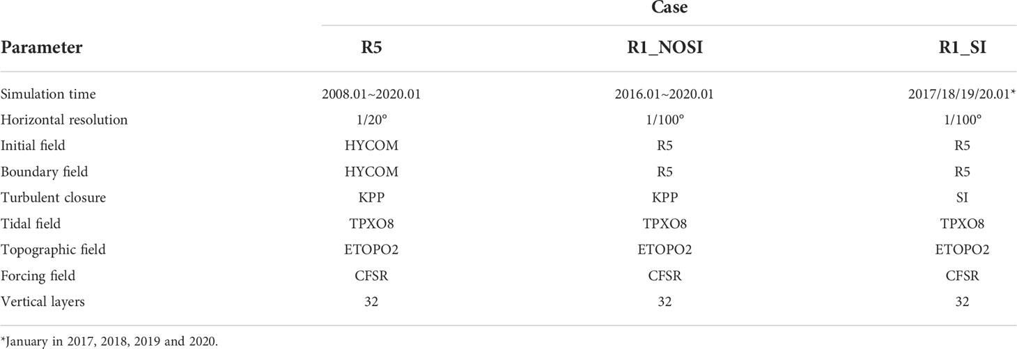
The Xisha-Zhongsha waters are constructed according to the method of one-way offline nesting (Mason et al., 2010). The parent domain, named R5, has a range of 9°~25°N, 105°~128°E with a horizontal resolution of ~5km and a temporal resolution of 1day. The nested grid, named R1, is 14°~18°N, 111°~117°E whose horizontal and temporal resolutions are ~1km and ~6hours, respectively. (Figure 1). R5 and R1 have 32 layers vertically, with more layers concentrated near the surface. The topography is provided by NOAA with a spatial resolution of 2’. We used data for model setup on potential temperature, salinity, currents and sea surface height obtained from the HYCOM reanalysis data for the period of 2008 to 2020. The horizontal resolution is 1/12°, and there are 40 layers (from 2008 to 2012) and 41 layers (from 2013 to 2020) vertically. The atmospheric forcing data of the model are from the National Centers for Environmental Prediction (NCEP) Climate Forecast System Reanalysis (CFSR) for the period of 2008 to 2010 and its second edition, Climate Forecast System Version 2 (CFSV2) for the period of 2011 to 2020. The spatial resolutions of the two versions are 0.312°×0.312° and 0.205°×0.204°, respectively, and temporal resolution is both 6 hours, including air temperature at 2m height above ground, specific humidity, precipitation, wind speed at 10m height above ground, long and short wave flux, etc. The simulation includes tidal forcing, which is particularly critical in the SCS where tides play a key role in many aspects of regional dynamics (Wang et al., 2017; Lin et al., 2020; Yan et al., 2020). The tidal data used in this study are from TPXO8. The tidal data of the model is derived from TPXO8 with a 1/30° horizontal resolution, including eight main tidal components: M2, S2, K1, O1, N2, P1, K2 and Q1.
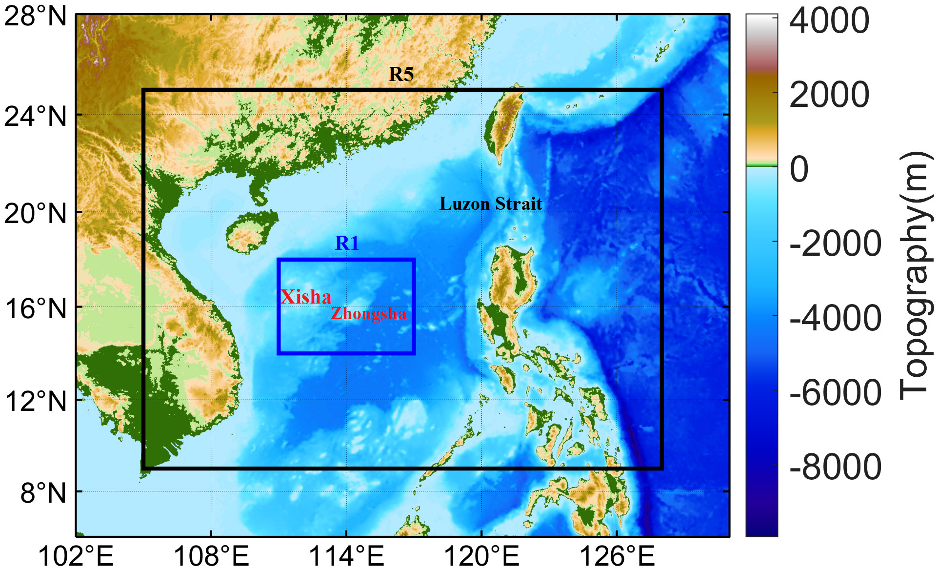
Figure 1 Topography of simulated area (unit: m). The black and blue lines denote the parent and nested domains, R5 and R1, respectively.
For R5, the initial field and open boundary are from the HYCOM reanalysis data, while the surface fluxes are derived from CFSR. In order to obtain the relatively stable initial field for R1, R5 is simulated for 11 years, from January 1, 2008 to January 31, 2020 (the KE and potential energy of R5 reach stability quickly after several months; not shown). Based on the R5 results R1 is simulated for approximately 4 years, from January 1, 2016 to January 31, 2020. Two contrast cases are carried out to highlight the SI effects from the SI scheme. One uses the KPP scheme, named R1_ NOSI. The other one applies the SI scheme together with the KPP, i.e., R1_SI. Considering that SI is more active in winter (Dong et al., 2021a), only results in January from 2017 to 2020 are analyzed here. Details of the model setup are shown in Table 1.
2.4 Model validation
Since the nested high-resolution simulation is carried out on the basis of R5 results, it is necessary to verify the performance of R5 simulation. Here, the SST and circulation pattern averaged in January are investigated and compared with observations and reanalysis data. The SST from R5 decreases from southeast to northwest, which is basically consistent with the distribution of OISST (Figures 2A, B). In terms of the circulation, the surface, middle and deep layers of R5 show cyclonic, anticyclonic and cyclonic patterns, respectively (Figures 2C, D), which resembles the HYCOM reanalysis result. The sandwichlike inflow–outflow–inflow pattern is also consistent with previous studies arguing the three-layer alternating rotation structure of the SCS circulation (Wyrtki, 1961; Tian et al., 2006; Liu et al., 2008; Wang et al., 2011; Lan et al., 2013).
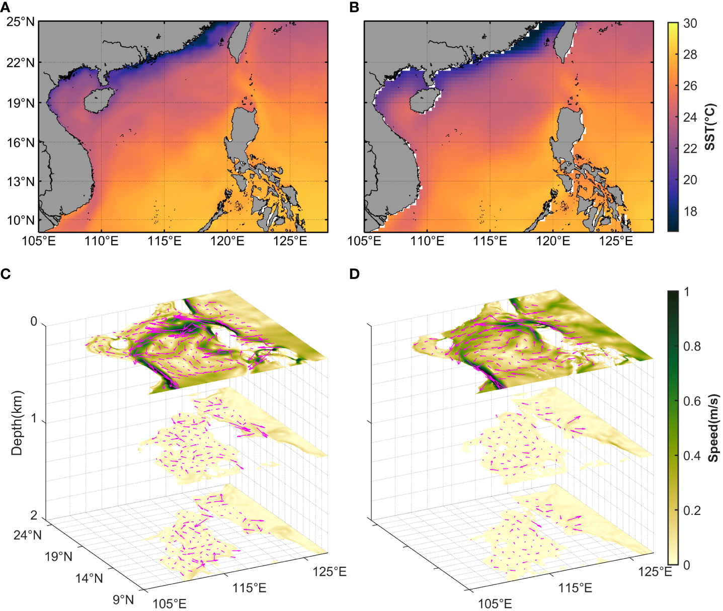
Figure 2 The monthly average SST in R5 of (A) the result of our model, (B) the OISST, and the monthly average circulation of 0m, 1000m and 2000m horizontal layers of (C) the result of our model, (D) the result of HYCOM reanalysis data. Both velocity arrows at 1000m depth and 2000m depth are magnified by 5 times. The monthly average refers to the monthly average in January from 2017 to 2020.
As for R1, the submesoscale process caused by MLI and frontogenesis are resolved, although the resolution cannot directly resolve SI. Taking a snapshot on January 8th, 2018 as an instance, the distribution of temperature and horizontal gradient of density at the depth of 5m from R1_NOSI simulation (Figures 3A, B) shows that frontal processes are active in R1, and eddies with a horizontal radius of O (10~ 100) km are also observed. Further, according to the distribution of the Rossby number (the vertical relative vorticity normalized by the local planetary vorticity, ζ) at the depth of 5m (Figure 3C), dynamic processes with Rossby number of about 1 are widely observed in the upper layer. The Rossby number even reaches larger than 2 in areas with complex background dynamic processes, such as the sea area around the Xisha Islands with sharp frontal and topographic changes. The density horizontal gradient (∣∇ρh∣) presents a good correlation with the Rossby number. Areas with strong Rossby number and active submesoscale processes are generally accompanied by strong fronts. In addition, the strong Rossby number in the upper layer usually indicates strong vertical velocities. According to the vertical velocity at 20m (Figure 3D), it can be seen that the vertical velocity can reach 100 meters day-1. The above phenomena and characteristics are consistent with the law of submesoscale processes obtained from observations (Zhong et al., 2017; Zhang et al., 2021).
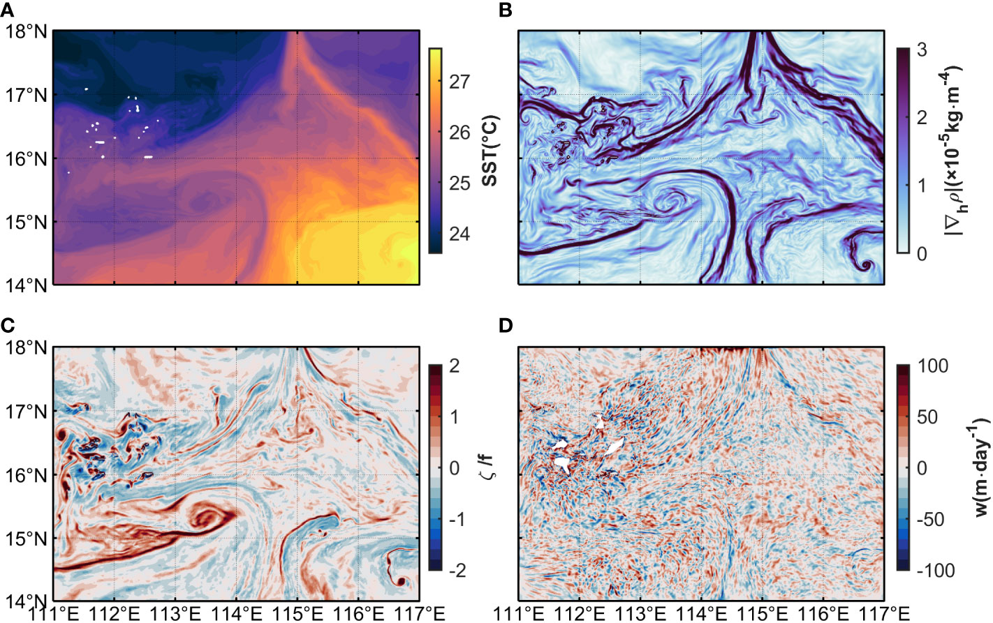
Figure 3 Snapshots of (A) the horizontal temperature at 5m water depth, (B) the horizontal gradient of density at 5m water depth, (C) the vertical relative vorticity at 5m water depth, and (D) the vertical velocity at 20m water depth of R1 at 18:00 on January 8th, 2018.
2.5 Definition and distribution characteristics of symmetric instability activity
The activity of forced SI in the simulation domain can be firstly investigated based on the criterion:fq<0,B0>0, and EBF>0. Based on the 6-hourly output of snapshots in R1_NOSI, the probability distribution of SI activity in January of each year is shown (Figure 4). Overall, high probabilities of SI are observed in Xisha-Zhongsha waters during this period, with values generally larger than 10% in most regions (even larger than 30% in some regions). It is worth mentioning that SI activity always has a high probability near the Xisha Islands with complex topography, which should be a result of strong submesoscale fronts (cf. Figure 3) due to current-topography interactions (Dewar et al., 2015; Molemaker et al., 2015; Gula et al., 2016). Here, the effect of SI will be highlighted by comparing regions with SI in R1_SI to that in R1_NOSI.

Figure 4 Probability distribution of SI activity in January (A) 2017, (B) 2018, (C) 2019 and (D) 2020. Inside the blue rectangle are the Xisha Islands. SI, symmetric instability.
3 Effects of symmetric instability
3.1 Effects on energetics
This section mainly assesses the effect of the SI scheme on GSP, the effective input of wind energy and the rate of the energy release of larger scale APE to the submesoscale via buoyancy production.
The contribution of SI to the forward ocean energy cascade is non-negligible because the KE extracted by SI from geostrophic shear is transferred to smaller scales (Taylor and Ferrari, 2010; D’Asaro et al., 2011; Buckingham et al., 2019; Yu et al., 2019). Therefore, the effect of SI on GSP can be highlighted by comparing GSP in these two cases. Combined with the thermal wind balance (fk x ǝug/ǝz=∇hbb), GSP can be calculated by
where v is the vertical viscosity coefficient from the model output, and bb is the background component of buoyancy [c.f. Equation (12) for details]. Using the horizontal background buoyancy gradient to diagnose the flow field based on geostrophic balance can eliminate the interference of internal tide to a certain extent. Figure 5 shows the vertical profiles of GSP for the two cases in January. The calculated GSP is nearly zero below the SML but positive in the SML, implying frontal geostrophic shear energy is consumed. However, the magnitude of GSP from R1_SI is 2-3 times that of R1_NOSI in the SML (within about 30 meters, see the section 3.2 for details), indicating that the dissipation of geostrophic shear is enhanced by SI and roughly agrees with the result in an idealized frontal experiment (Dong et al., 2021b). This GSP enhancement is a result of the greater viscosity due to SI parameterization scheme. These results indicate that the SI parameterization scheme can enhance the dissipation of geostrophic KE and transport energy towards a smaller scale but above the scale of Kolmogorov dissipation (Su et al., 2016). In other words, SI promotes the forward cascade of energy and the SI scheme mimic this behavior successfully. It is worth noting that the depth corresponding to the peak value moves up by approximately 3m compared with R1_NOSI in each year. We can find that the GSP in R1_SI is greater than that in R1_NOSI at any time if we integrate the GSP in the upper 50m in each year (Figure 6). Note that there is a good correspondence between the trends of the GSP difference (magenta line) and GSP itself (R1_SI in red and R1_NOSI in blue), which is understandable because the stronger the vertical shear of the geostrophic current at the front in R1_NOSI, the more of GSP is extracted from the nearby SI, causing the greater GSP in R1_SI at the same time.
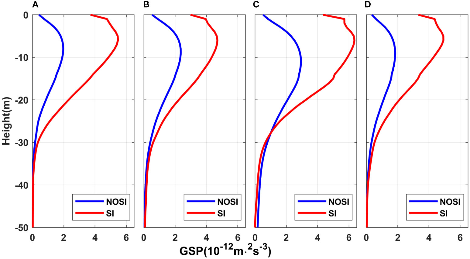
Figure 5 The domain-averaged vertical profile of GSP in January (A) 2017, (B) 2018, (C) 2019, (D) 2020. GSP, geostrophic shear production.
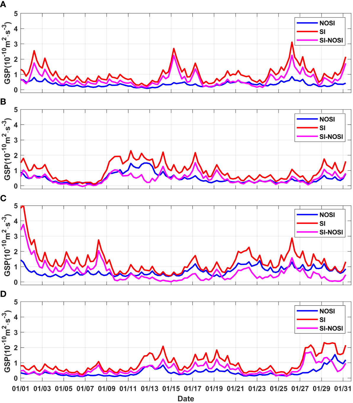
Figure 6 The time series of the GSP and GSP difference of two cases in the upper 50 m in January (A) 2017, (B) 2018, (C) 2019, (D) 2020. GSP, geostrophic shear production.
Due to the change of geostrophic currents by SI, the effective input of wind work is speculated to be modulated. The effect of SI on the wind work input can be calculated by
where, τw and us is the sea surface wind stress and velocity respectively. Figure 7 shows the time series of the wind work input (R1_SI in red and R1_NOSI in blue) and the difference (orange line) in January for each year. Qualitatively, there is a good relationship between ΔP and P (the orange line trend is almost the opposite of the blue line trend), that is, when the wind work is greater, the effect of the SI scheme on wind work weakening is more significant. This is because when the wind blows in the direction of geostrophic current (down-front winds), the SI at around fronts weakens the fronts, and the geostrophic current ug is weakened, causing a decrease in the value of us. As shown in Figure 7, the stronger the ug at the front, the more significant the effect of the SI scheme on GSP dissipation. This process eventually leads to a reduction of the usable wind work (i.e., the rate of geostrophic component of KE increase in coherent motions due to down-front winds) done on fronts under forced SI. Quantitatively, the average ∆P account for 5.9%, 7.9%, 6.2% and 4.8% of the averaged wind work input in R1_NOSI from 2017 to January 2019, respectively (even up to 15% at certain times).
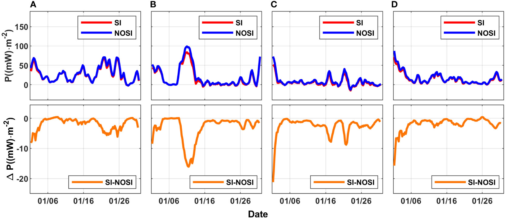
Figure 7 The time series of the wind work input P and ∆P of two cases in SI activity region in January (A) 2017, (B) 2018, (C)2019, (D) 2020.
The conversion of APE to KE in the SML is mainly associated with MLI in the simulation. To assess it, the spatial scale of MLI LMLI is determined by (Dong et al., 2020a),
Here, R is the baroclinic Rossby deformation radius in the SML, NML and HML are the averaged buoyancy frequency and mixed layer depth (MLD) over the domain. LMLI is calculated as about 30km, which is taken as the cut-off scale to decompose the velocity and buoyancy fields by spatially filtering into background (large- and mesoscale) and submesoscale components:
The rate of the energy release of larger scale APE to the submesoscale via buoyancy production can be evaluated by
The overline here represents spatio-temporally averaging. The domain vertical profiles of PK with or without the SI parameterization scheme are shown in Figure 8. PK approaches zero near the sea surface and increases first and then decreases with the increase of depth. Different from GSP that is mainly intensified in the SML at the jet, PK tends to energize the whole mixed layer and reaches its maximum in the middle of the mixed layer, which is consistent with the theory of Fox-Kemper et al. (2008) and Cao et al. (2021). However, SI changes the PK peak value and the corresponding depth. In R1_NOSI, the peak value of PK is at a water depth of 10~20m while 10~15m in R1_SI, that is, the depth of the peak value has moved up by approximately 5m. This phenomenon may covary with the mixed layer restratification caused by SI (it will be discussed further in Section 4.1). The peak value of PK is suppressed by about half as the SI effects are included. In brief, PK tends to be weakened after the SI parameterization scheme is applied. The vertical integral of PK over 0~30m is also weakened (Figure 9). Note that the weakening degree of PK seems to be dependent on PK itself (the magenta line trend is opposite to the blue line trend). The larger the value of PK is, the more significant the inhibition effect of the SI parameterization seems to be, even exceeding 50% around the peak value. It can be concluded that the SI parameterization scheme inhibits the buoyancy production. This inhibition may be a result of the background KE dissipation by SI. As the background KE at fronts is decreased due to SI growing, fronts tend to be weakened, and the APE is potentially decreased and converted to background KE via geostrophic adjustment. The weakened fronts are speculated to suppress PK. The effect suggests an interaction between SI and MLI or frontogenesis, which is still an open question and will not be discussed in the work.
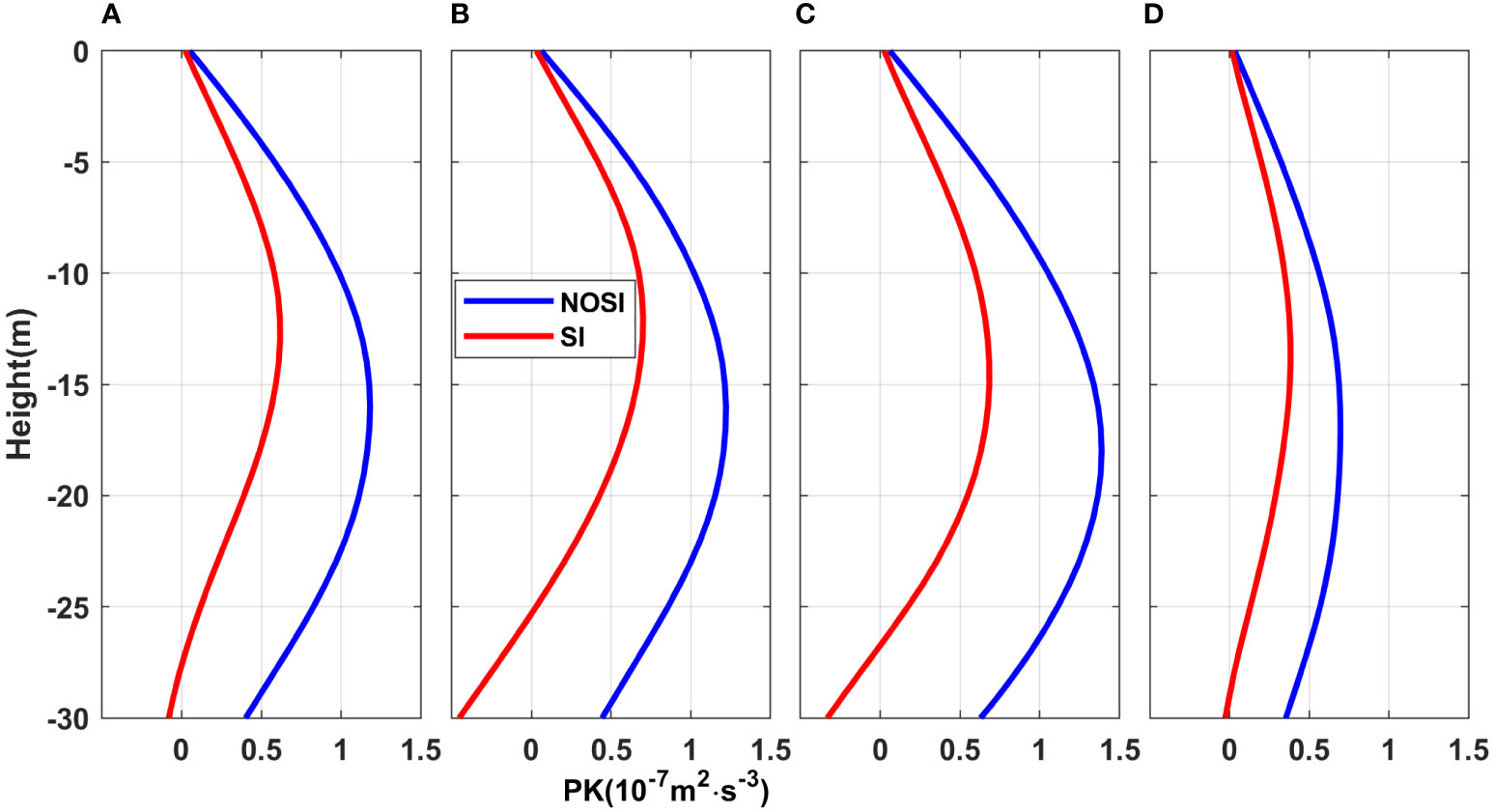
Figure 8 The domain-averaged vertical profiles of PK in January, (A) 2017, (B) 2018, (C) 2019, (D) 2020. PK, the rate of the energy release of larger scale APE to the submesoscale via buoyancy production.
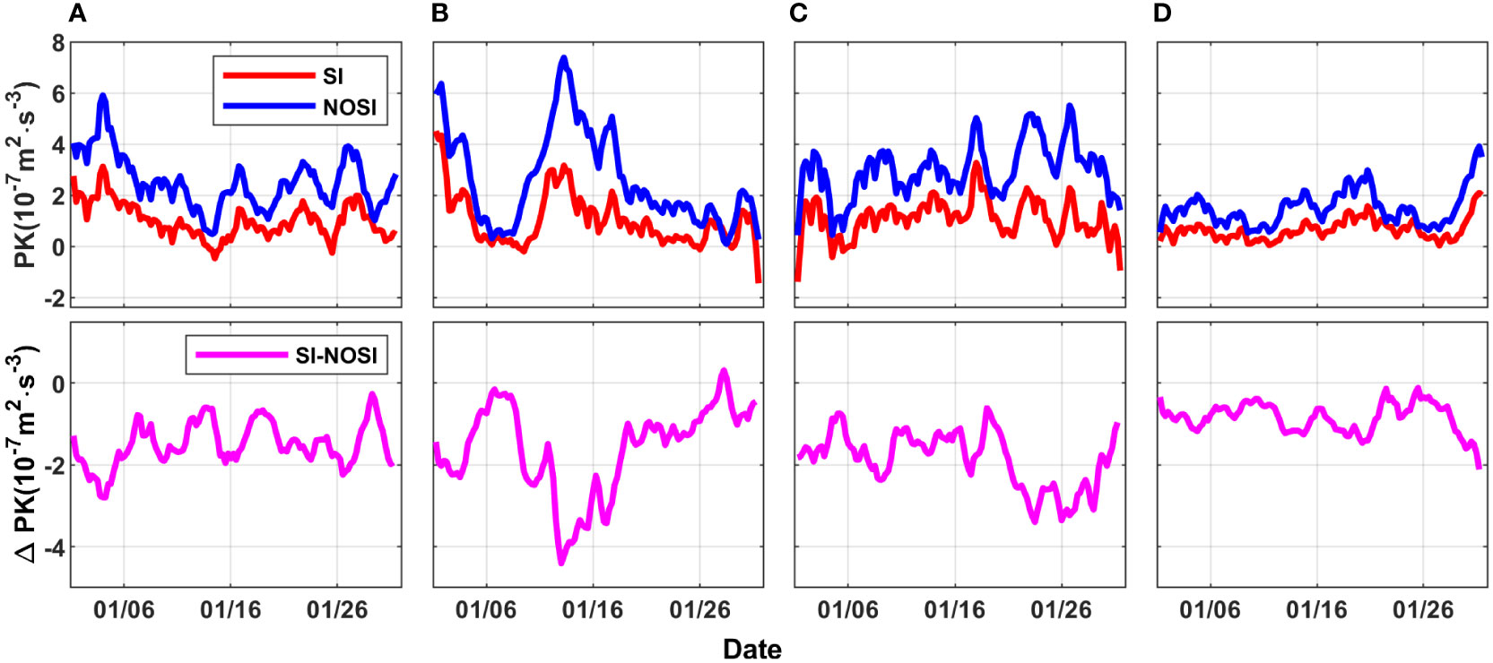
Figure 9 The time series of the PK and PK difference of two cases in the upper 30 m in January (A) 2017, (B) 2018, (C) 2019, (D) 2020. PK, the rate of the energy release of larger scale APE to the submesoscale via buoyancy production.
3.2 Mixed layer depth and sea surface temperature
According to D21, SI tends to restratify the mixed layer and then shoal the MLD. The dynamic mechanisms for this phenomenon are as follows: before SI occurs, the original isopycnals are generally inclined and PV is negative. To restore PV to a neutral state (i.e., PV = 0) and reach marginal SI stability, the local water masses overturn and mix until the isopycnals become flat at the fronts. Therefore, the mixed layer is restratified (Bachman and Taylor, 2014; Bachman et al., 2017). Figure 10A shows the MLD difference of the two cases at the same time as Figure 3. The MLD is determined with a threshold potential density value of 0.03 kg m-3 (de Boyer Montégut et al., 2004). According to Figures 10A, C, it can be seen that the area of the shoaled MLD has a good relationship with the SI activity region with shoaling magnitudes up to 5 m.
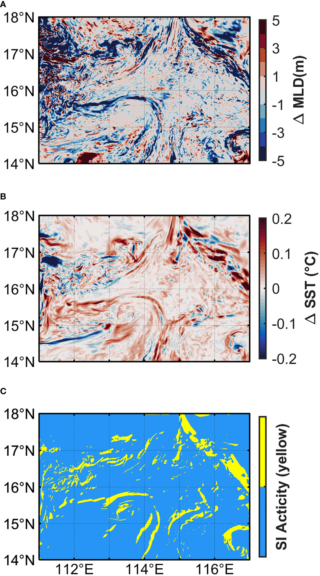
Figure 10 (A) MLD difference (SI-NOSI), (B) SST difference (SI-NOSI) of the two cases and (C) distribution of SI activity (Filled in yellow for SI activity and blue for SI inactivity) at the same time as Figure 3.
We compare the performance of the two cases in simulating the MLD with the MLD derived from HYCOM reanalysis. Figure 11 shows the MLD time series of the two cases (R1_NOSI in bule and R1_SI in red, respectively) in January for each year, and the reanalysis MLD (green line) in the corresponding month. Overall, R1_SI is closer to the observed MLD than R1_NOSI, indicating an improvement of the MLD simulation due to the SI scheme. To more specifically quantify the improvement, we introduce a root mean square error (RMSE) metric. RMSE is a measure to evaluate how close the model’s MLD is to the reanalysis one and is defined as:
where MLDmodel and MLDobs are the model’s MLD (R1_NOSI or R1_SI) and the reanalysis one, respectively; n is the total number of the days in corresponding month. The results illustrate that SI parameterization reduces the RMSE of MLD by 14.32%, 12.47%, 22.83% and 21.52% (Supplementary Figure 2).
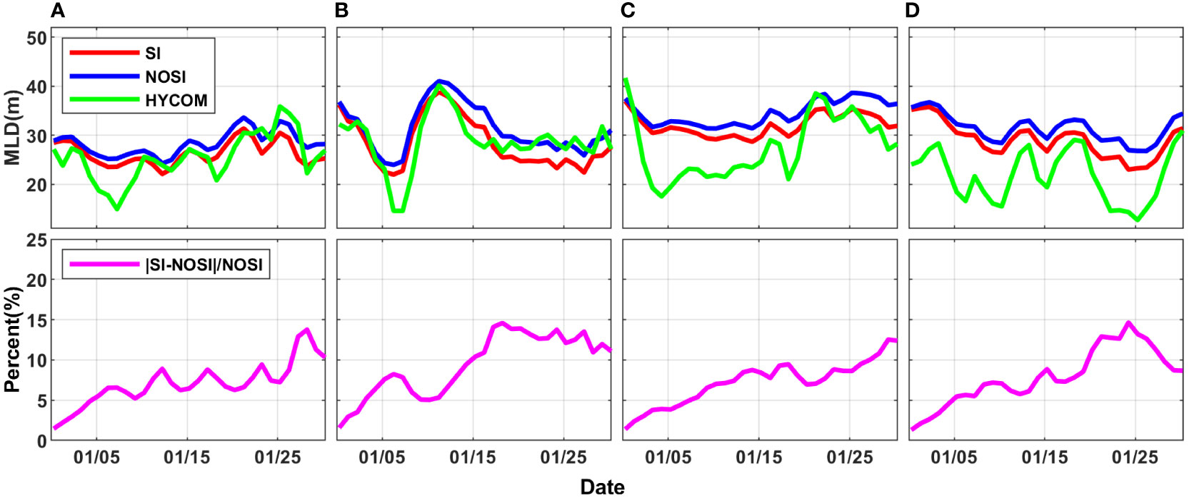
Figure 11 The time series of the domain-averaged MLD from the simulations (blue and red line for R1_NOSI and R1_SI, respectively) and the proportion of the MLD difference (magenta line) to the one from R1_NOSI in January (A) 2017, (B) 2018, (C) 2019, (D) 2020. The concurrent MLD from the reanalysis is shown as the green line.
The shoaling of the MLD suggests that the SI parameterization scheme well represents the restratification effect of SI. The magenta line in Figure 11 shows the proportion of the MLD reduction of R1_SI relative to R1_NOSI. Within 20 days after the application of SI parameterization scheme, the reduced proportion increases almost linearly with time, and tends to be dynamic stable after 20 days, with values between 10~15%.
The restratification of the SML caused by SI makes the originally inclined isopycnals tend to be horizontal, so that the seawater with relatively lower temperature and higher density sinks, and then the sea surface temperature potentially rises. Taking the snapshot at the same time as Figure 3 as an example, Figure 10B shows the SST differences. It can be seen that the areas where SST increases are mostly concentrated in the SI activity region (Figure 10C), and the anomalies in some regions can even exceed 0.5°C. In addition, the average SST difference in January from 2017 to 2020 is shown in Figure 12. Although most of the differences are within the range of 0.1°C, the SST of R1_SI is relatively higher than R1_NOSI. Since any assimilation based on observations is not implemented, the SST is different from observations in fine patterns (not shown). Therefore, here only shows the indirect impact of SI on SST, rather than emphasizing the improvement of simulated SST.
3.3 Ertel potential vorticity analysis
A direct impact from SI is the ability to reduce negative PV and restore PV to a neutral state. PV can be further assessed for examining specific impacts of SI on PV in the stratified and rotational flows. According to Cao and Jing (2022), we assume that the large-scale mean flows are dominant in geostrophic balance and the horizontal gradients of vertical velocity are negligible. On basis of Equation (1), PV can be further decomposed into two components ash
where (f + ζ)bz is the vertical vorticity component, qvert, and (k x uz) ∇h b is the baroclinic component, qbc. As in Equation (14), both the vorticity and the baroclinicity play important roles in stimulating instability at the front with strong strain. Taking a snapshot of PV distribution at the same time as Figure 3 as an instance (Figure 13), the two components of PV in the two cases are compared at depths of 5 m (representing the SML). The vertical vorticity component, qvert, tends to be the positive dominant constituent for PV in most of the regions, while is nearly zero near the fronts, indicative of reduced PV for ongoing instabilities. On the contrary, the baroclinic component, qbc, exhibits strong negative filamentous structures in the fronts, which is favorable for SI events. There is a correspondence between this pattern and horizontal density gradient in Figure 3B, which arises from submesoscale frontogenesis (Cao and Jing, 2022). Therefore, in the SML, the instability near the fronts is mainly modulated by the negative PV from the baroclinic component, while PV in other regions is dominated by the vertical vorticity component. The above leads to that there are alternating patterns of positive and negative PV values in the SML, and the negative PV mainly exits in the region with large horizontal density gradient.
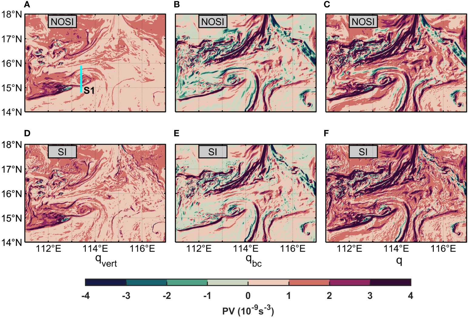
Figure 13 Comparison of the near-surface (at 5m water depth) Ertel PV q and its sub-components in different cases. The panels (A–F) show snapshots in R1_NOSI (R1_SI) at the same time as Figure 3. The panels (A, D) are the vertical vorticity component of Ertel PV. The panels (B, E) are the baroclinic component of Ertel PV. The panels (C, F) are the Ertel PV. The S1 is selected for analyzing the vertical distribution of Ertel PV. PV, potential vorticity.
Through the comparison of Figures 13A,D, it can be found the magnitude of the positive PV is increased near the fronts and islands. Moreover, compared with R1_NOSI, the region of negative qbc in R1_SI is noticeably reduced. The patterns representing negative qbc also become much more fragmented and closer to zero (Figure 13E), as SI is expected to bring up stratified thermocline waters to oppose surface forcing and approach marginal stability for SI—zero PV. The S1 is selected for analyzing the vertical distribution of Ertel PV in the Discussion Section. Overall, the SI scheme changes the PV through elevating positive qvert and eliminating negative qbc.
According to the calculated time series of the probability of negative PV and the probability difference in the upper 5m in January from the two cases (Figure 14), it can be seen that the negative PV probability is mostly within 2%-10% in R1_NOSI (blue line), and reduced by 10%~50% relative to R1_NOSI in most of the time. We note that the trend of the negative PV probability difference resembles the one of the negative PV, and the time period in which the SI parameterization scheme greatly eliminates the negative PV corresponds to the time period in which the probability of the negative PV in R1_NOSI is high. The SI scheme can eliminate nearly half of the negative PV In other words, it implies that the ability of the SI scheme to eliminate negative PV seems to be positively related to the probability of negative PV itself in SML. When the probability of negative PV is at its maximum in the current month, the SI scheme can eliminate nearly half of the negative PV when the probability of negative PV reaches its maximum.
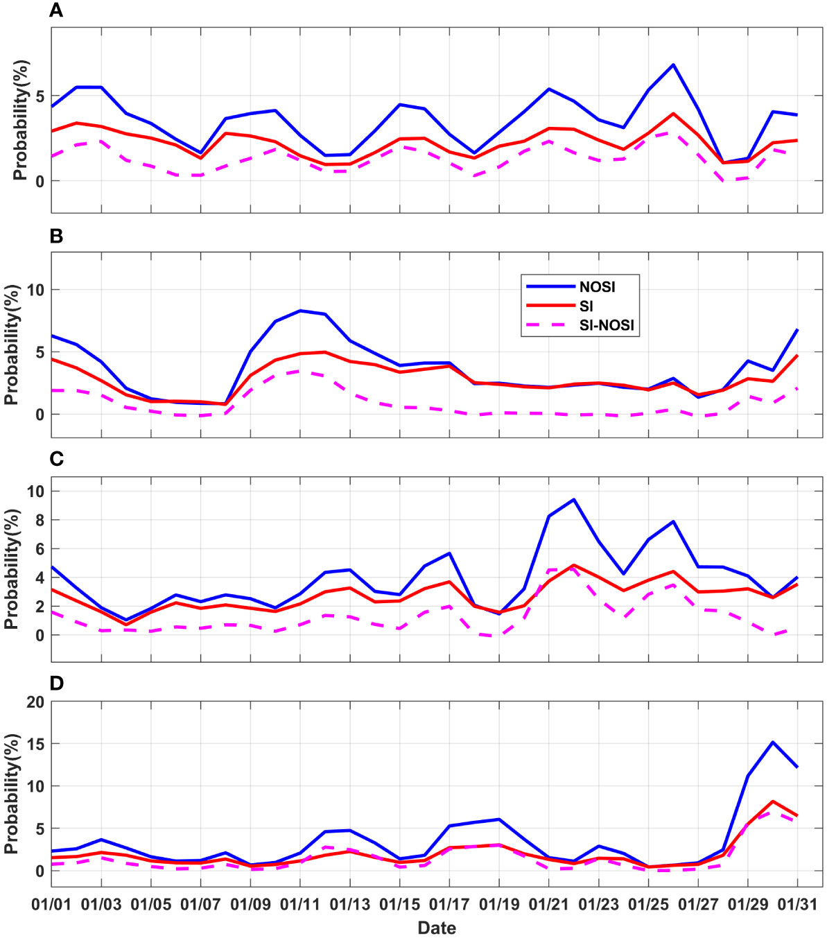
Figure 14 The time series of negative PV probability (blue and red line for R1_NOSI and R1_SI, respectively) and its difference (SI-NOSI, magenta line) in the upper 5m of two cases in January (A) 2017, (B) 2018, (C) 2019, (D) 2020. PV, potential vorticity.
4 Discussion and conclusions
4.1 Discussion
4.1.1 Effects around islands
In this work, we find that SI are more active at the Xisha islands with complex topography than the open water (cf. Figure 3 and Supplementary Figure 3). Therefore, we further select the Xisha islands region and an open water region in R1 (Supplementary Figure 3) and carry out a comparative analysis. It is found that the domain-averaged vertical profile of GSP in the Xisha domain is 6-7 times higher than that of the open water region (Supplementary Figure 4). In terms of the negative PV probability (Supplementary Figure 5), compared to the result of R1_NOSI, a remarkable reduction in the negative PV in the Xisha domain is observed (Supplementary Figure 5A), while it is almost unchanged in the open water (Supplementary Figure 5B). It indicates that the effects of the SI scheme are more noticeable around islands. This may be due to the current-topography interactions stimulate negative PV, providing favorable conditions for the SI activity.
4.1.2 Discussion on PK, PV and disturbance of internal tides
Although the MLD covaries with PK, this correlation doesn’t seem to be the only reason for the SML restratification. The SML restratification is induced by SI as well in two ways: the upward buoyancy flux—PK—shoals the SML, and SI tends to flatten isopycnals to reduce negative PV, leading to SML restratification (Dong et al., 2021b; Jing et al., 2021). We can see that the SI scheme tends to inhibits PK (Figures 8, 9) moderately—in other words—we surely overestimate the impact of energy conversion of the APE stored in the fronts when SI is not considered. However, the MLD is still much shallower in general (Figure 11) when SI is parameterized. The total changes may be attributed to the fact that the influence of SML restratification induced by SI as parameterized exceeds that of suppression of PK caused by SI. Furthermore, the MLD is reduced by about 15% in R1_SI, which may bring up the dynamic instability mechanisms in the SML to a shallower depth, eventually leading to the shallower depth of the peaks of GSP and PK vertical profile (Figures 5, 8). In addition, although PK is suppressed, it is unexpected that there is a little more submesoscale component of KE in R1_SI (not shown), indicating that the impact of SI on the model may be more systematic and complex, and the reasons for it need to be further studied.
Further insight into the vertical profiles of Ertel PV is conducive to understanding the impacts of the SI scheme on negative PV (the S1 marked in Figure 13A). The S1 crosses the mesoscale cyclonic eddy and exhibits negative PV within the mixed layer (Supplementary Figure 6). The negative qvert only exits in the middle and base of the mixed layer, because the deepened pycnocline in the eddy core largely strengths the qvert by the intensification of density stratification. Notice that in most regions, the qbc acts to balance the qvert field, and the negative q is mainly contributed by qbc. The PV with opposite signs to the Coriolis frequency for flows is favorable for the development of SI that can drive large vertical motions, ultimately leading to restratification through enhanced mixing. Then the effect of the SI scheme is presented by comparing the two cases. The SI scheme increases the vertical vorticity component of PV and shallows the MLD (highlighted by the blue solid rectangles in Supplementary Figures 6A, D), while restore the baroclinic component of PV to a neutral state (highlighted by the blue solid rectangles in Supplementary Figures 6B, E). This further confirms the conclusions in Section 3.3. However, it seems that the role of the SI scheme in weakening the negative baroclinic component of PV is not limited to the SML, which needs more specific research in the future.
In addition, taking GSP as an instance, we also compare whether the SI parameterization effects are affected by the internal tides signal. In order to remove the internal tides signals, a 2-day low-pass filter (fourth-order Butterworth) was therefore applied to the time series, according to Zhang et al. (2021). Supplementary Figure 7 shows time series of GSP with and without filtering. It indicates that the internal tides seem to only have a subtle impact on the results but do not change the conclusions in Section 3.1. This may be because the main effects of SI parameterization are in the SML, while the influence of internal tides is mainly below the mixed layer. The stratification in the mixed layer is weak, so the impact of internal tides is relatively moderate. Besides, according to Thomas et al. (2016), although the energetics of SI interacting with inertial motions is transient, the average within inertial periods can be ignored.
4.1.3 Discussion on realistic implementation
In this study, we mainly focus on the impacts of SI in a regional model, but the limitation of the scheme should be noted. One of the prerequisites for activating the SI scheme is that both B0 and EBF are positive (Supplementary Figure 1), implying not all forced SI is parameterized (the forced SI only requires B0 + EBF> 0). Hence, it may underestimate the SI impacts. According to the result from an idealized frontal experiment (Dong et al., 2021b), SI can occur at the front with a strong positive EBF when B0 is negative. If a more general scheme of SI is adopted, the effects of SI is expected to be amplified. In addition, we only analyse the SI effect in January and its seasonality is not evaluated. However, since we know that SI is one of the important submesoscale instabilities, according to the research results of Cao et al. (2022) on the submesoscale seasonality in the SCS, the submesoscale processes in the middle ocean basin (which partially coincides with the R1 region in this study) are seasonal and more active in winter, which is mainly due to the winter wind shear and frontal effect. Another more direct evidence is the SI events assessed by Dong et al. (2021a), the relative likelihood of SI events is correspondingly high in winter. In addition, compared with other seasons, the SCS has deeper MLD and weaker stratification in winter. Heat loss of seawater also tends to occur (i.e., B0 <0). All above are conducive to the occurrence of SI events in winter, implying that the effects of SI in other seasons is more moderate than that in winter.
The effect of SI parameterization depends on the ability of the model to resolve mesoscale and submesoscale fronts. However, most of the widely used regional models are only mesoscale resolving (dx = 10 km) at present. For these models, it is necessary to firstly extend the coarse resolution to the fine resolution through some methods, and then apply the SI parameterization. According to (1), (5), and (6), SI parameterization depends on the horizontal density gradient, while coarser models have weaker gradients than finer. According to Fox-Kemper et al. (2011), a rescaling can be done with some confidence based on an analysis of the horizontal wavenumber spectrum of near-surface density variance. That is, the coarse-resolution models need to be added a scaling factor Δs/Lf to improve weaker density gradients (Δsis the local coarse model gridscale dimension and Lf is an estimate of the typical local width of mixed layer fronts), and a mixing timescale T to handle behavior near the equator. The specific resolution to be expanded depends on the scale of the local MLI.
4.2 Conclusion
In this work, the SI scheme proposed by B17 is applied in the CROCO with a realistic configuration alongside the KPP scheme in Xisha-Zhongsha waters, probability of SI activity in most region exceeds 10% and is even over 40% in some region in January. The model simulations with SI parameterization applied shows that the SI parameterization makes marked impacts on real simulation in winter.
In energetics, the application of SI parameterization has increased GSP more than doubled, successfully expressing the extraction effect of SI on GSP and reflecting the forward energy cascade of SI. It moderately reduces the wind work further by weakened geostrophic current. The PK is reassessed when considering SI and we find the SI scheme also suppresses approximately half of the energy conversion of larger scale APE to the submesoscale. The reasons for this mechanism need further study in the future.
The SI scheme has remarkably improved the simulation of MLD, making it shallower by 10%~15% through restratifying, and more similar to the observation. Compared with the case without SI, the RMSE between the MLD depth obtained by mode simulation and the reanalysis one is reduced by 12% ~ 25%. The effect on MLD further caused an increase within 1°C in SST, which reaches the same magnitude order as the average SST anomaly in this region. Another indirect effect of restratification of mixed layer is that the depth of the peak value of GSP and PK in vertical profiles is reduced by 3 ~ 5m.
By Ertel PV analysis, we find that in the SML, the instability near the fronts is mainly modulated by the negative PV from the baroclinic component, while the PV in other regions is dominated by the vertical vorticity component. The SI scheme changes the PV through elevating positive qvert and eliminating negative qbc, leading to reducing the probability of the negative PV by 10%~ 50% in the SML. In addition, the effects of SI around islands are more significant than that in open water region, indicating the importance of SI scheme in complex topography.
This work here demonstrates that the SI scheme has a good performance in representing the SI effect in valuable tool that covers the impact of SI in realistic simulation. According to the theory of Fox-Kemper et al. (2011), the SI scheme may be able to applied in the current widely used (mesoscale resolving) models. However, the tracers of nutrients have not been released in this model, so the impact of the SI scheme on nutrients exchanges between the SML and the ocean interior in the realistic model has not been studied. In addition, when we assess the impact of SI on wind work, the influence of sea surface roughness is not considered in the model. Overall, further studies of higher-resolution simulation and field observations are required to solve the above problems.
Data availability statement
The OISST analyzed for this study can be found in the https://www.ncei.noaa.gov/products/optimum-interpolation-sst/. The dataset of HYCOM analyzed for model setup can be found in the https://www.hycom.org/dataserver/. The HYCOM reanalysis MLD data were downloaded from http://hycom.org/dataserver/glb-reanalysis/. The dataset of CFSR and CFSV2 analyzed for this study can be found in the https://rda.ucar.edu/datasets/ds093.0/ and https://rda.ucar.edu/datasets/ds094.0/, respectively. The dataset of topography analyzed for this study can be found in the http://www.ngdc.noaa.gov/mgg/global/global.html/. The dataset of TPXO8 analyzed for this study can be found in the https://www.tpxo.net/global/tpxo8-atlas/. The CROCO and CROCO_TOOLS are provided by http://www.croco-ocean.org, and the code of the SI scheme is available at https://github.com/jhdong2016/SI_model.
Author contributions
YJ conducted the numerical simulation test, performed the data analysis and wrote the manuscript. XZ and JD conceived the study and contributed to the editing of the manuscript. XZ and HW initiated the idea of the study. WJZ conducted a supervisory review. WMZ provided resource support and project administration. All authors contributed to the analysis of the results and writing the manuscript.
Funding
This study was supported by the National Key Research and Development Program (Grants 2021YFC3101504), and the National Natural Science Foundation of China (42176023 and 42276205).
Acknowledgments
We would like to thank the editor and the two reviewers for their valuable comments.
Conflict of interest
The authors declare that the research was conducted in the absence of any commercial or financial relationships that could be construed as a potential conflict of interest.
Publisher’s note
All claims expressed in this article are solely those of the authors and do not necessarily represent those of their affiliated organizations, or those of the publisher, the editors and the reviewers. Any product that may be evaluated in this article, or claim that may be made by its manufacturer, is not guaranteed or endorsed by the publisher.
Supplementary material
The Supplementary Material for this article can be found online at: https://www.frontiersin.org/articles/10.3389/fmars.2022.985605/full#supplementary-material
References
Anderson P. S. (2009). Measurement of prandtl number as a function of Richardson number avoiding self-correlation. Boundary-Layer Meteorol. 131 (3), 345–362. doi: 10.1007/s10546-009-9376-4
Bachman S. D., Fox-Kemper B., Taylor J. R., Thomas L. N. (2017). Parameterization of frontal symmetric instabilities. I: Theory for resolved fronts. Ocean Model. Online 109, 72–95. doi: 10.1016/j.ocemod.2016.12.003
Bachman S. D., Taylor J. R. (2014). Modelling of partially-resolved oceanic symmetric instability. Ocean Model. Online 82, 15–27. doi: 10.1016/j.ocemod.2014.07.006
Buckingham C. E., Lucas N. S., Belcher S. E., Rippeth T. P., Grant A. L. M., Le Sommer J., et al. (2019). The contribution of surface and submesoscale processes to turbulence in the open ocean surface boundary layer. J. Adv. Model. Earth Syst. 11 (12), 4066–4094. doi: 10.1029/2019MS001801
Cao H., Fox-Kemper B., Jing Z. (2021). Submesoscale eddies in the upper ocean of the kuroshio extension from high-resolution simulation: energy budget. J. Phys. Oceanogr. 51 (7), 2181–2201. doi: 10.1175/JPO-D-20-0267.1
Cao H., Jing Z. (2022). Submesoscale ageostrophic motions within and below the mixed layer of the northwestern pacific ocean. J. Geophys. Res.: Ocean. 127 (2), e2021JC017812. doi: 10.1029/2021JC017812
Cao H., Meng X., Jing Z., Yang X. (2022). High-resolution simulation of upper-ocean submesoscale variability in the south China Sea: Spatial and seasonal dynamical regimes. Acta Oceanol. Sin. 41 (7), 26–41. doi: 10.1007/s13131-022-2014-4
Cao X., Shi H., Shi M., Guo P., Wu L., Ding Y., et al. (2017). Model-simulated coastal trapped waves stimulated by typhoon in northwestern south China Sea. J. Ocean Univ. China 16 (6), 965–977. doi: 10.1007/s11802-017-3255-2
Capet X., McWilliams J. C., Molemaker M. J., Shchepetkin A. F. (2008). Mesoscale to submesoscale transition in the California current system. part III: Energy balance and flux. J. Phys. Oceanogr. 38 (10), 2256–2269. doi: 10.1175/2008jpo3810.1
D’Asaro E., Lee C., Rainville L., Harcourt R., Thomas L. (2011). Enhanced turbulence and energy dissipation at ocean fronts. Science 332 (6027), 318–322. doi: 10.1126/science.1201515
de Boyer Montégut C., Madec G., Fischer A. S., Lazar A., Iudicone D. (2004). Mixed layer depth over the global ocean: An examination of profile data and a profile-based climatology. J. Geophys. Res.: Ocean. 109, C12003. doi: 10.1029/2004JC002378
Dewar W. K., McWilliams J. C., Molemaker M. J. (2015). Centrifugal instability and mixing in the California undercurrent. J. Phys. Oceanogr. 45 (5), 1224–1241. doi: 10.1175/jpo-d-13-0269.1
Dong J., Fox-Kemper B., Zhang H., Dong C. (2020a). The scale of submesoscale baroclinic instability globally. J. Phys. Oceanogr. 50 (9), 2649–2667. doi: 10.1175/jpo-d-20-0043.1
Dong J., Fox-Kemper B., Zhang H., Dong C. (2020b). The seasonality of submesoscale energy production, content, and cascade. Geophys. Res. Lett. 47 (6), e2020GL087388. doi: 10.1029/2020GL087388
Dong J., Fox-Kemper B., Zhang H., Dong C. (2021a). The scale and activity of symmetric instability estimated from a global submesoscale-permitting ocean model. J. Phys. Oceanogr. 51 (5), 1655–1670. doi: 10.1175/jpo-d-20-0159.1
Dong J., Fox-Kemper B., Zhu J., Dong C. (2021b). Application of symmetric instability parameterization in the coastal and regional ocean community model (CROCO). J. Adv. Model. Earth Syst. 13 (3), e2020MS002302. doi: 10.1029/2020MS002302
Fox-Kemper B., Danabasoglu G., Ferrari R., Griffies S. M., Hallberg R. W., Holland M. M., et al. (2011). Parameterization of mixed layer eddies. III: Implementation and impact in global ocean climate simulations. Ocean Model. Online 39 (1), 61–78. doi: 10.1016/j.ocemod.2010.09.002
Fox-Kemper B., Ferrari R., Hallberg R. (2008). Parameterization of mixed layer eddies. part I: Theory and diagnosis. J. Phys. Oceanogr. 38 (6), 1145–1165. doi: 10.1175/2007JPO3792.1
Gula J., Molemaker M. J., McWilliams J. C. (2016). Topographic generation of submesoscale centrifugal instability and energy dissipation. Nat. Commun. 7 (1), 12811. doi: 10.1038/ncomms12811
Haine T. W. N., Marshall J. (1998). Gravitational, symmetric, and baroclinic instability of the ocean mixed layer. J. Phys. Oceanogr. 28 (4), 634–658. doi: 10.1175/1520-0485(1998)028<0634:Gsabio>2.0.Co;2
Ho C.-R., Kuo N.-J., Zheng Q., Soong Y. S. (2000). Dynamically active areas in the south China Sea detected from TOPEX/POSEIDON satellite altimeter data. Remote Sens. Environ. 71 (3), 320–328. doi: 10.1016/S0034-4257(99)00094-2
Huang X., Jing Z., Zheng R., Cao H. (2020). Dynamical analysis of submesoscale fronts associated with wind-forced offshore jet in the western south China Sea. Acta Oceanol. Sin. 39 (11), 1–12. doi: 10.1007/s13131-020-1671-4
Huang B., Liu C., Banzon V., Freeman E., Graham G., Hankins B., et al. (2021). Improvements of the daily optimum interpolation Sea surface temperature (DOISST) version 2.1. J. Clim. 34 (8), 2923–2939. doi: 10.1175/jcli-d-20-0166.1
Hu J., Kawamura H., Hong H., Kobashi F., Wang D. (2001). 3≈6 months variation of Sea surface height in the south China Sea and its adjacent ocean. J. Oceanogr. 57 (1), 69–78. doi: 10.1023/A:1011126804461
Hu J., Kawamura H., Hong H., Qi Y. (2000). A review on the currents in the south China Sea: Seasonal circulation, south China Sea warm current and kuroshio intrusion. J. Oceanogr. 56 (6), 607–624. doi: 10.1023/A:1011117531252
Jing Z., Fox-Kemper B., Cao H., Zheng R., Du Y. (2021). Submesoscale fronts and their dynamical processes associated with symmetric instability in the Northwest pacific subtropical ocean. J. Phys. Oceanogr. 51 (1), 83–100. doi: 10.1175/jpo-d-20-0076.1
Jullien S., Caillaud M., Benshila R., Bordois L., Cambon G., Dumas F., et al. (2019) Technical and numerical doc. Available at: https://www.croco-ocean.org/documentation/.
Lan J., Zhang N., Wang Y. (2013). On the dynamics of the south China Sea deep circulation. J. Geophys. Res.: Ocean. 118 (3), 1206–1210. doi: 10.1002/jgrc.20104
Large W. G., McWilliams J. C., Doney S. C. (1994). Oceanic vertical mixing: A review and a model with a nonlocal boundary layer parameterization. Rev. Geophys. 32 (4), 363–403. doi: 10.1029/94RG01872
Lin H., Liu Z., Hu J., Menemenlis D., Huang Y. (2020). Characterizing meso- to submesoscale features in the south China Sea. Prog. Oceanogr. 188, 102420. doi: 10.1016/j.pocean.2020.102420
Liu Q., Kaneko A., Jilan S. (2008). Recent progress in studies of the south China Sea circulation. J. Oceanogr. 64 (5), 753–762. doi: 10.1007/s10872-008-0063-8
Liu Z., Lozovatsky I. (2012). Upper pycnocline turbulence in the northern south China Sea. Chin. Sci. Bull. 57 (18), 2302–2306. doi: 10.1007/s11434-012-5137-8
Li J., Zheng Q., Hu J., Fan Z., Zhu J., Chen T., et al. (2015). Wavelet analysis of coastal-trapped waves along the China coast generated by winter storms in 2008. Acta Oceanol. Sin. 34 (11), 22–31. doi: 10.1007/s13131-015-0701-0
Li J., Zheng Q., Hu J., Xie L., Zhu J., Fan Z. (2016). A case study of winter storm-induced continental shelf waves in the northern south China Sea in winter 2009. Cont. Shelf Res. 125, 127–135. doi: 10.1016/j.csr.2016.06.013
Luo S., Jing Z., Qi Y. (2020). Submesoscale flows associated with convergent strain in an anticyclonic eddy of the kuroshio extension: A high-resolution numerical study. Ocean Sci. J. 55 (2), 249–264. doi: 10.1007/s12601-020-0022-x
Mahadevan A. (2006). Modeling vertical motion at ocean fronts: Are nonhydrostatic effects relevant at submesoscales? Ocean Model. Online 14 (3-4), 222–240. doi: 10.1016/j.ocemod.2006.05.005
Mason E., Molemaker J., Shchepetkin A. F., Colas F., McWilliams J. C., Sangrà P. (2010). Procedures for offline grid nesting in regional ocean models. Ocean Model. Online 35 (1), 1–15. doi: 10.1016/j.ocemod.2010.05.007
McWilliams J. C. (2016). Submesoscale currents in the ocean. Proc. R. Soc. A: Math. Phys. Eng. Sci. 472 (2189), 20160117. doi: 10.1098/rspa.2016.0117
Mellor G. L., Yamada T. (1982). Development of a turbulence closure model for geophysical fluid problems. Rev. Geophys. 20 (4), 851–875. doi: 10.1029/RG020i004p00851
Molemaker M. J., McWilliams J. C., Dewar W. K. (2015). Submesoscale instability and generation of mesoscale anticyclones near a separation of the California undercurrent. J. Phys. Oceanogr. 45 (3), 613–629. doi: 10.1175/jpo-d-13-0225.1
Park J.-H., Farmer D. (2013). Effects of kuroshio intrusions on nonlinear internal waves in the south China Sea during winter. J. Geophys. Res.: Ocean. 118 (12), 7081–7094. doi: 10.1002/2013JC008983
Qu T., Kim Y. Y., Yaremchuk M., Tozuka T., Ishida A., Yamagata T. (2004). Can Luzon strait transport play a role in conveying the impact of ENSO to the south China Sea? J. Clim. 17 (18), 3644–3657. doi: 10.1175/1520-0442(2004)017<3644:Clstpa>2.0.Co;2
Redi M. H. (1982). Oceanic isopycnal mixing by coordinate rotation. J. Phys. Oceanogr. 12 (10), 1154–1158. doi: 10.1175/1520-0485(1982)012<1154:Oimbcr>2.0.Co;2
Su Z., Ingersoll A. P., Stewart A. L., Thompson A. F. (2016). Ocean convective available potential energy. part I: Concept and calculation. J. Phys. Oceanogr. 46 (4), 1081–1096. doi: 10.1175/jpo-d-14-0155.1
Sun Z., Zhang Z., Qiu B., Zhou C., Zhao W., Tian J. (2022). Subsurface mesoscale eddies observed in the northeastern south China Sea: Dynamic features and water mass transport. J. Phys. Oceanogr. 52 (5), 841–855. doi: 10.1175/jpo-d-21-0177.1
Su Z., Torres H., Klein P., Thompson A. F., Siegelman L., Wang J., et al. (2020). High-frequency submesoscale motions enhance the upward vertical heat transport in the global ocean. J. Geophys. Res.: Ocean. 125 (9), e2020JC016544. doi: 10.1029/2020JC016544
Su Z., Wang J., Klein P., Thompson A. F., Menemenlis D. (2018). Ocean submesoscales as a key component of the global heat budget. Nat. Commun. 9 (1), 775. doi: 10.1038/s41467-018-02983-w
Taylor J. R., Ferrari R. (2010). Buoyancy and wind-driven convection at mixed layer density fronts. J. Phys. Oceanogr. 40 (6), 1222–1242. doi: 10.1175/2010jpo4365.1
Thomas L. N. (2005). Destruction of potential vorticity by winds. J. Phys. Oceanogr. 35 (12), 2457–2466. doi: 10.1175/jpo2830.1
Thomas L. N., Taylor J. R., Ferrari R., Joyce T. M. (2013). Symmetric instability in the gulf stream. Deep Sea Res. Part II: Top. Stud. Oceanog. 91, 96–110. doi: 10.1016/j.dsr2.2013.02.025
Thomas L. N., Taylor J. R., D’Asaro E. A., Lee C. M., Klymak J. M., Shcherbina A. (2016). Symmetric instability, inertial oscillations, and turbulence at the Gulf Stream front. J. Phys. Oceanogr. 46 (1), 197–217. doi: 10.1175/jpo-d-15-0008.1
Thompson A. F., Lazar A., Buckingham C., Naveira Garabato A. C., Damerell G. M., Heywood K. J. (2016). Open-ocean submesoscale motions: A full seasonal cycle of mixed layer instabilities from gliders. J. Phys. Oceanogr. 46 (4), 1285–1307. doi: 10.1175/jpo-d-15-0170.1
Tian J., Yang Q., Liang X., Xie L., Hu D., Wang F., et al. (2006). Observation of Luzon strait transport. Geophys. Res. Lett. 33 (19). doi: 10.1029/2006GL026272
Umlauf L., Burchard H. (2003). A generic length-scale equation for geophysical turbulence models. J. Mar. Res. 61 (2), 235–265. doi: 10.1357/002224003322005087
Wang X., Liu Z., Peng S. (2017). Impact of tidal mixing on water mass transformation and circulation in the south China Sea. J. Phys. Oceanogr. 47 (2), 419–432. doi: 10.1175/JPO-D-16-0171.1
Wang G., Xie S.-P., Qu T., Huang R. X. (2011). Deep south China Sea circulation. Geophys. Res. Lett. 38 (5). doi: 10.1029/2010GL046626
Wyrtki K. (1961). Physical Oceanography of the Southeast Asian waters. UC San Diego: Library – Scripps Digital Collection. doi: 10.1017/S0025315400054370
Xie L., Zheng Q., Tian J., Zhang S., Feng Y., Yi X. (2016). Cruise observation of rossby waves with finite wavelengths propagating from the pacific to the south China Sea. J. Phys. Oceanogr. 46 (10), 2897–2913. doi: 10.1175/jpo-d-16-0071.1
Yang Q., Zhao W., Liang X., Dong J., Tian J. (2017). Elevated mixing in the periphery of mesoscale eddies in the south China Sea. J. Phys. Oceanogr. 47 (4), 895–907. doi: 10.1175/jpo-d-16-0256.1
Yan T., Qi Y., Jing Z., Cai S. (2020). Seasonal and spatial features of barotropic and baroclinic tides in the northwestern south China Sea. J. Geophys. Res.: Ocean. 125 (1), e2018JC014860. doi: 10.1029/2018JC014860
Yu X., Naveira Garabato A. C., Martin A. P., Gwyn Evans D., Su Z. (2019). Wind-forced symmetric instability at a transient mid-ocean front. Geophys. Res. Lett. 46 (20), 11281–11291. doi: 10.1029/2019GL084309
Zhang Z., Tian J., Qiu B., Zhao W., Chang P., Wu D., et al. (2016). Observed 3D structure, generation, and dissipation of oceanic mesoscale eddies in the south China Sea. Sci. Rep. 6 (1), 24349. doi: 10.1038/srep24349
Zhang Z., Zhang Y., Qiu B., Sasaki H., Sun Z., Zhang X., et al. (2020). Spatiotemporal characteristics and generation mechanisms of submesoscale currents in the northeastern south China Sea revealed by numerical simulations. J. Geophys. Res.: Ocean. 125 (2), e2019JC015404. doi: 10.1029/2019JC015404
Zhang Z., Zhang X., Qiu B., Zhao W., Zhou C., Huang X., et al. (2021). Submesoscale currents in the subtropical upper ocean observed by long-term high-resolution mooring arrays. J. Phys. Oceanogr. 51 (1), 187–206. doi: 10.1175/jpo-d-20-0100.1
Zhang Z., Zhao W., Qiu B., Tian J. (2017). Anticyclonic eddy sheddings from kuroshio loop and the accompanying cyclonic eddy in the northeastern south China Sea. J. Phys. Oceanogr. 47 (6), 1243–1259. doi: 10.1175/jpo-d-16-0185.1
Zhang Z., Zhao W., Tian J., Liang X. (2013). A mesoscale eddy pair southwest of Taiwan and its influence on deep circulation. J. Geophys. Res.: Ocean. 118 (12), 6479–6494. doi: 10.1002/2013JC008994
Zheng Q., Ho C.-R., Xie L., Li M. (2019). A case study of a kuroshio main path cut-off event and impacts on the south China Sea in fall-winter 2013–2014. Acta Oceanol. Sin. 38 (4), 12–19. doi: 10.1007/s13131-019-1411-9
Zheng Q., Tai C.-K., Hu J., Lin H., Zhang R.-H., Su F.-C., et al. (2011). Satellite altimeter observations of nonlinear rossby eddy–kuroshio interaction at the Luzon strait. J. Oceanogr. 67 (4), 365–376. doi: 10.1007/s10872-011-0035-2
Zhong Y., Bracco A., Tian J., Dong J., Zhao W., Zhang Z. (2017). Observed and simulated submesoscale vertical pump of an anticyclonic eddy in the south China Sea. Sci. Rep. 7 (1), 1–13. doi: 10.1038/srep44011
Keywords: submesoscale, symmetric instability, parameterization, regional models, South China Sea, oceanic mixed layer, potential vorticity
Citation: Jiang Y, Dong J, Zhang X, Zhang W, Wang H and Zhang W (2022) Evaluating the effects of a symmetric instability parameterization scheme in the Xisha-Zhongsha waters, South China Sea in winter. Front. Mar. Sci. 9:985605. doi: 10.3389/fmars.2022.985605
Received: 04 July 2022; Accepted: 13 September 2022;
Published: 03 October 2022.
Edited by:
Zhiyu Liu, Xiamen University, ChinaCopyright © 2022 Jiang, Dong, Zhang, Zhang, Wang and Zhang. This is an open-access article distributed under the terms of the Creative Commons Attribution License (CC BY). The use, distribution or reproduction in other forums is permitted, provided the original author(s) and the copyright owner(s) are credited and that the original publication in this journal is cited, in accordance with accepted academic practice. No use, distribution or reproduction is permitted which does not comply with these terms.
*Correspondence: Xiaojiang Zhang, emhhbmd4aWFvamlhbmcxOUBudWR0LmVkdS5jbg==; Huizan Wang, d2FuZ2h1aXphbjE3QG51ZHQuZWR1LmNu
 Yifei Jiang
 Jihai Dong
 Xiaojiang Zhang
 Wenjing Zhang1
 Weimin Zhang