Rapid reconstruction of temperature and salinity fields based on machine learning and the assimilation application

Satellite observations play important roles in ocean operational forecasting systems, however, the direct assimilation of satellite observations cannot provide sufficient constraints on the model underwater structure. This study adopted the indirect assimilation method. First, we created a 3D temperature and salinity reconstruction model that took into account the advantage of the nonlinear regression of the generalized regression neural network with the fruit fly optimization (abbreviated as FOAGRNN). Compared with the reanalysis product and the WOA13 climatology data, the synthetic T/S (temperature and salinity) profiles had sufficient accuracy and could better describe the characteristics of mesoscale eddies. Then, the synthetic T/S profiles were assimilated into the Regional Ocean Model System (ROMS) using the Incremental Strong constraint 4D Variational (I4D-Var) data assimilation algorithm. The quantitative and qualitative analysis results indicated that compared with the direct assimilation of satellite observations, the root mean square errors (RMSEs) of temperature and salinity were reduced by 26.0% and 23.1% respectively by assimilating the synthetic T/S profiles. Furthermore, this method significantly improved the simulation effect of the model underwater structure, especially in the 300 m to 500 m water layer. Compared with the National Marine Data Center’s real-time analysis data, the machine learning-based assimilation system demonstrated a significant advantage in the simulation of underwater salinity structure, while showing a similar performance in the simulation of underwater temperature structure.

1 Introduction

By combining observations and numerical models, data assimilation not only can make up for the temporal discontinuity and spatial inhomogeneity of observations but also can improve the accuracy of numerical models. However, the effect of data assimilation depends on the quality of the observations and their spatiotemporal distribution. With the development of satellite technology, satellite data have experienced incredible growth (Ratheesh et al., 2012). Sea surface temperature (SST) and sea level anomaly (SLA) have become the indispensable data in operational systems, and the assimilation of sea surface salinity (SSS) can also enhance the forecasting effect on El Niño/Southern Oscillation (ENSO) (Tranchant et al., 2019). Compared with ship surveys or buoys, satellite can provide large-scale observations of the ocean surface with better time continuity. However, satellite cannot directly observe the subsurface, and the adjustment of the underwater structure of numerical models still relies on the observations of T/S profiles by instruments such as Argo buoys. However, the in-situ observations like Argo buoys are scarce. For example, only one Argo buoy was active in the South China Sea on May 18, 2018.

How to use satellite data to constrain the subsurface temperature and salinity structure is a complex problem in ocean data assimilation. One method is statistical, which establishes statistical relationships between surface and subsurface seawater states, including multiple linear regression and Empirical Orthogonal Functions (EOFs). Carnes et al. (1994) determined the EOF magnitude of the vertical temperature structure as a function of SST and sea surface height (SSH) by performing multivariate least squares regression on more than 33,000 historical T/S profiles in the Northwest Pacific and Northwest Atlantic Oceans. In this way, they projected the observation information of SST and SSH underwater. Based on the work of Carnes et al. (1994); Fox et al. (2002) developed the Modular Ocean Data Assimilation System (MODAS) and applied it to the US Navy Coupled Ocean Data Assimilation (NCODA) system. To reduce significant errors near the thermocline layer, the US Navy established an Improved Synthetic Ocean Profiles (ISOP) system. The system divided the ocean into mixed layers, thermocline, and quiescent layers. The vertical mapping model of the T/S profiles was established respectively by using multiple regression, one-dimensional variational data assimilation, and linear regression at three levels (Helber et al., 2013). Following the practice of the US Navy, China’s National Marine Data Center successfully established MODAS and ISOP systems and used them to produce real-time analysis data. This approach proposed by Carnes et al. (1994) is not suitable for areas where observations are scarce. To address this problem, Ezer and Mellor (1994) utilized model output to establish the statistical relationship between the sea surface height anomaly and the subsurface temperature and salinity anomaly. Then they assimilated the data from satellite tracks to improve the temperature structure of the 500 m water layer. The simulation effect of this method is dependent on the performance of the model. In the ensemble method, the ensemble samples can also be employed to consider the relationship between the surface and the subsurface layers, and then the observation information can be passed down (Chen et al., 2018; Zhou et al., 2021).

Different from the statistical method, the dynamic method uses dynamic constraints to transfer the sea surface information downward. Common dynamic methods include the nudging approach (Holland and Malanotte-Rizzoli, 1989; Chen et al., 2020) and the dynamic conservation technique (Haines, 1991; Cooper and Haines, 1996; Weaver et al., 2005). In the Nudging approach, a nudging term is added to the right side of the dynamic equation, and the assimilated sea surface observation information is transferred to the deep layer only through the model dynamic framework. However, this approach may induce disturbances during the adjustment phase of the model, resulting in poor simulation of the subsurface structure (Cooper and Haines, 1996). In the dynamic conservation technique, the adjustment is performed based on the conservation properties or balance relationships of the ocean, such as potential vorticity conservation, geostrophic equilibrium, static equilibrium, etc. (Weaver et al., 2005; Liu et al., 2019; Liu et al., 2021). With the further development of the assimilation methods, the variational assimilation method was proposed. This method decomposes the assimilation increment into a balance term and a non-balance term. In the balance term, the balanced relationship is utilized to establish a multivariate balance operator to indirectly adjust the observed variables (Moore et al., 2011a; Moore et al., 2011b; Cummings and Smedstad, 2013). Dynamic conservation often adopts a simple dynamic framework, which is mainly suitable for adjusting the large-scale or small-scale components that satisfy the conservation relationship but is often not applicable to near shore.

In recent years, machine learning methods have been increasingly employed in meteorological and oceanographic applications, including bias correction of satellite observations (Vernieres et al., 2014; Le et al., 2020; Iqbal et al., 2022) and subsurface temperature and salinity reconstruction (Su et al., 2015; Chapman and Charantonis, 2017; Su et al., 2018; Bao et al., 2019). Compared with the multiple linear regression method used in MODAS, the machine learning method is more efficient in reconstruction and has a strong nonlinear regression capability and a high degree of fault tolerance and robustness. Bao et al. (2019) utilized the generalized regression neural network with fruit fly optimization (abbreviated as FOAGRNN) to reconstruct the salinity profiles based on sea surface data, and the reconstruction effect was better than that in multiple linear regression at the strong thermocline layer. To address the shortcomings of the direct assimilation for insufficient constraints on the model underwater structure, a machine learning-based assimilation system was established in this study. We first reconstructed the satellite observations into underwater 3D T/S pseudo-profiles using the FOAGRNN algorithm. Then we assimilated the synthetic profiles into the ROMS using the I4D-Var data assimilation algorithm. To validate the accuracy and effectiveness of this system, the system results were compared with the experiment results of the direct assimilation and the real-time analysis data of the National Marine Data Center.

The article is organized in the following sections: Section 2 describes the data sources, machine learning algorithms, assimilation methods, and model setup. Section 3 evaluates the accuracy of the FOAGRNN reconstruction model. Section 4 conducts three groups of assimilation experiments to examine the simulation effect of the machine learning-based assimilation system on the model underwater structure. Finally, a summary and a discussion of our research findings are given in Section 5.

2 Details of the machine learning-based assimilation system

Compared with the conventional method of the direct assimilation of satellite data, we created a machine learning-based assimilation system (Figure 1), which was divided into three main steps: in the first step, historical satellite altimeter data and historical T/S profiles were collected, and then the reconstruction model was obtained by training with the FOAGRNN algorithm proposed by Bao et al. (2019); in the second step, the assimilation time period was selected, and the real-time satellite observations were employed as the input field of the reconstruction model to construct the T/S profiles for each day; finally, the synthetic T/S profiles were assimilated into the model using the I4D-Var method. The data source, reconstruction methods, and assimilation system configuration are described below.

FIGURE 1

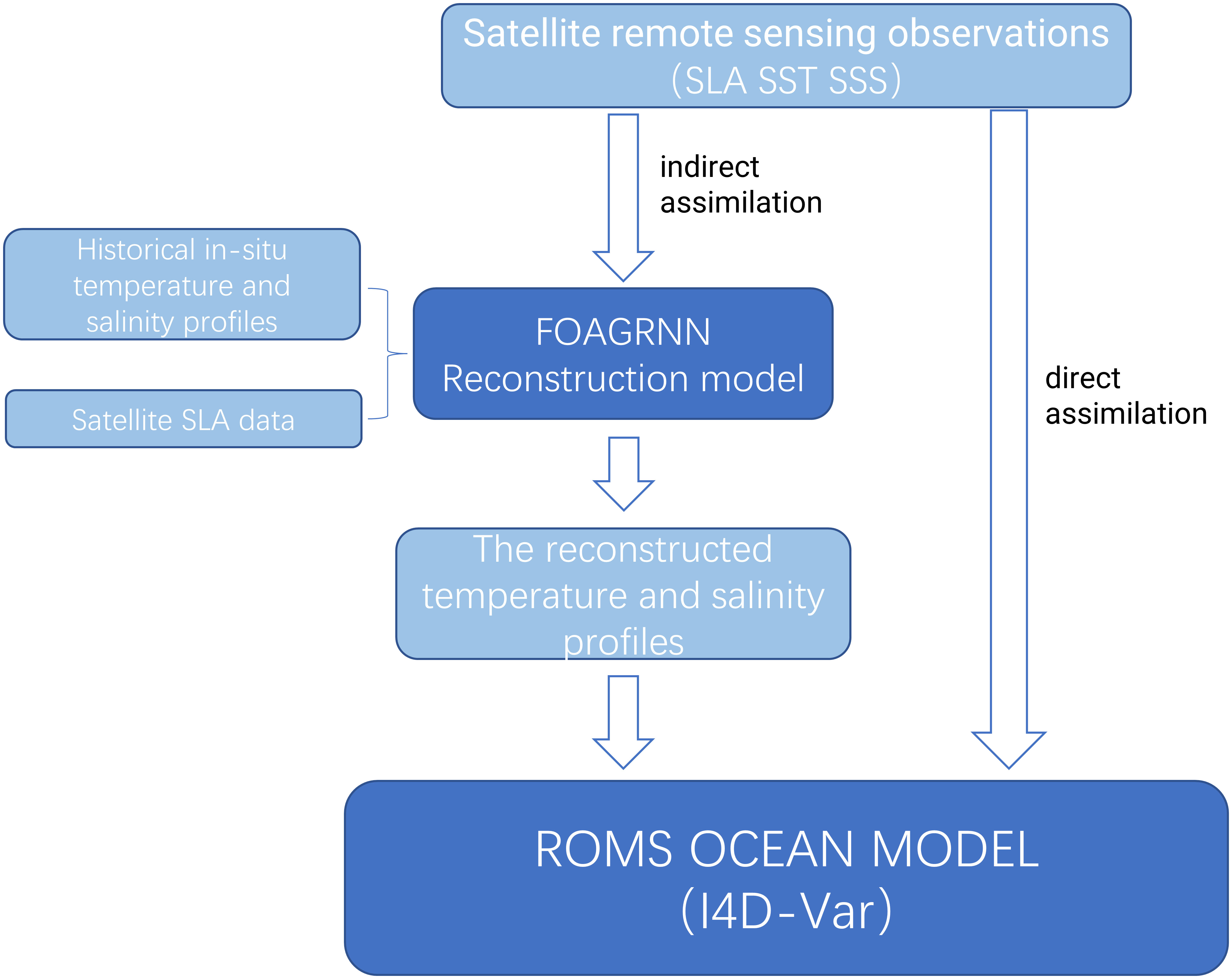
Figure 1 The flow chart of the machine learning-based assimilation system.

2.1 Data

The ocean observations used in this study included SLA, SST, SSS, and in situ observations. The satellite SLA data were delayed time and gridded maps of sea level anomaly (MSLA) from Copernicus Marine Environment Monitoring Service (CMEMS) with a horizontal resolution of 0.25°; the satellite SST data were acquired from the gridded product released by United Kingdom Meteorological Office (UKMO) with a horizontal resolution of 1/20° and were interpolated to SLA gridded points to maintain a consistent horizontal resolution (Good et al., 2020); the satellite SSS data were obtained from the Soil Moisture Active Passion (SMAP) with the same spatial and temporal resolutions as the SST and SLA data (He et al., 2021). All of the above satellite products had a temporal resolution of one day. In situ observations included the EN4.2.1 T/S profile datasets from the Hadley Center (Good et al., 2013), and survey data from the Northwest Pacific. The EN4.2.1 T/S profile datasets were divided into 24 layers at different depths, namely 2, 5.01, 15.07, 25.28, 35.7, 46.61, 57.98, 70.02, 82.92, 96.92, 112.32, 129.49, 148.96, 171.40, 197.79, 229.48, 268.46, 317.65, 381.39, 465.91, 579.31, 729.35, 918.37, and 1139.15 m. To ensure the accuracy of the reconstruction model, the historical satellite altimeter data and EN4.2.1 historical T/S profiles from 2004 to 2018 were used as the training data of the reconstruction model, and the corresponding data in 2019 were utilized as the test data. Each set of assimilation experiments corresponds to a reconstructed model. The numbers of the in-situ EN4.2.1 T/S profiles for training data and the test data were shown in Table 1, respectively. Satellite data (SLA, SST, SSS) from the assimilation period were employed as input fields for the reconstruction model to construct real-time 3D T/S pseudo-profiles. We also utilized WOA13 climatology data, SODA3.4.2 reanalysis product, GREP (Global Reanalysis multi-model Ensemble Product) and real-time analysis data of the National Marine Data Center (hereinafter referred to as MODAS) to evaluate the reconstruction model accuracy and assimilation effects (Carton et al., 2018; Storto et al., 2019). Survey data from the Northwest Pacific were used as independent observations for the qualitative analysis of the assimilation effect.

TABLE 1

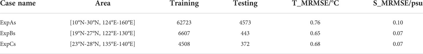
Table 1 The number of profiles being used for training and validation and the measurement error in the assimilation experiments.

2.2 Method

2.2.1 FOAGRNN

The Generalized Regression Neural Network (GRNN) is characterized by strong nonlinear mapping abilities, a flexible network structure, a high fault tolerance, and robustness. The theoretical basis of the GRNN is the nonlinear regression analysis. To maximize the effectiveness of GRNN, the key is the selection of smoothing parameters (Li et al., 2013). The fruit fly optimization algorithm is a new probabilistic method intended to find a global optimum based on the fruit fly’s foraging behaviors. By setting the cost function for iterative optimization, the error between the output value and the actual value is gradually reduced, so as to determine the optimal parameters. Many researchers have used the FOA to optimize the parameters of artificial neural network models (Lin, 2013). Taking GRNN as the research framework and using the FOA algorithm to determine the optimal smoothing parameters, Bao et al. (2019) proposed the FOAGRNN, which was employed to create the reconstruction model in our study. Taking the reconstructed model of ExpBs as example, the specific flow chart is shown in Figure 2 and the steps are as follows:

FIGURE 2

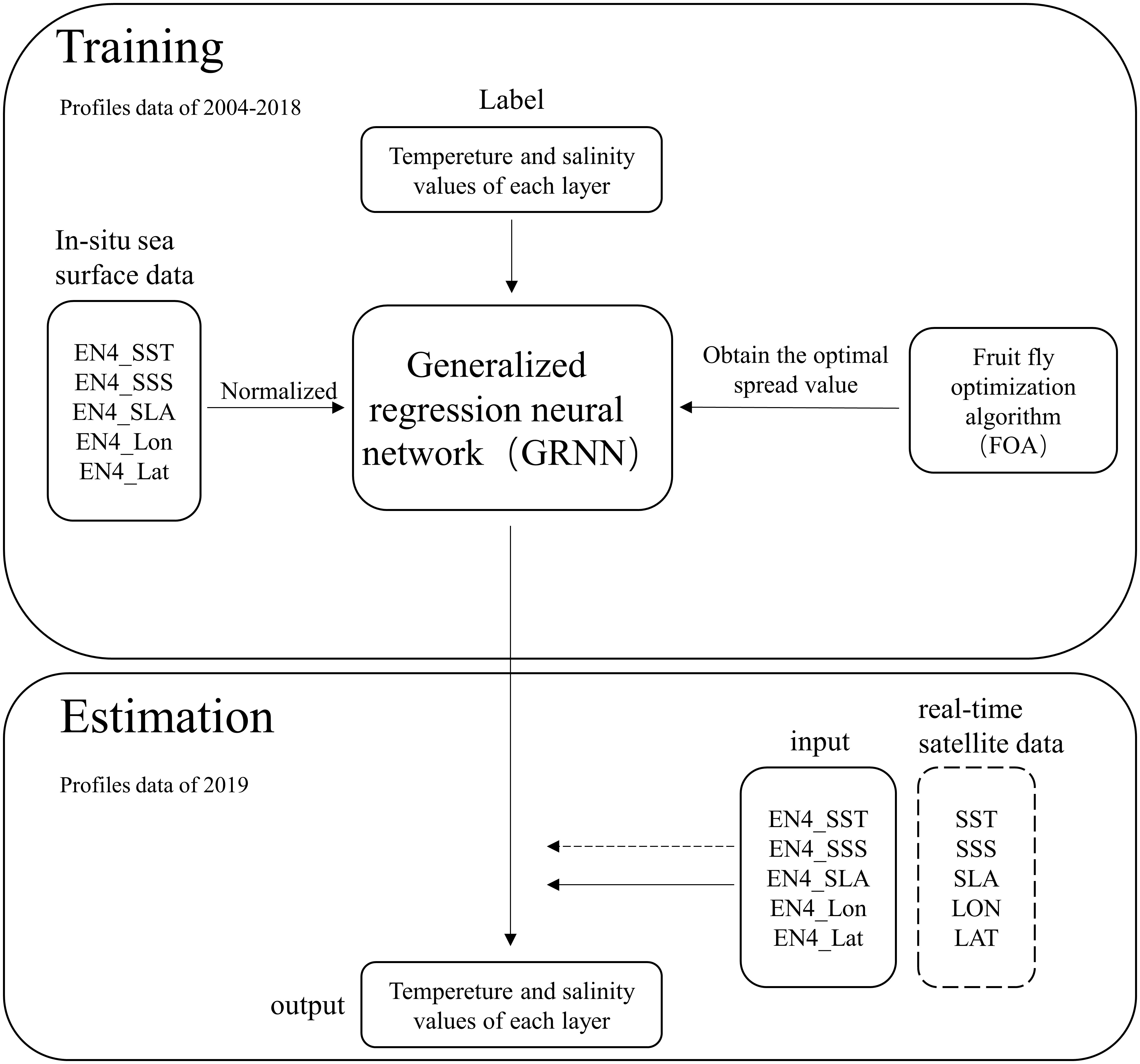
Figure 2 The flow chart of the reconstruction of 3D T/S profiles.

Step 1: Sample data preprocessing. The sample data included satellite altimeter data and in-situ EN4.2.1 T/S profiles. The spatial range of the selected sample data was [19°N-27°N, 122°E-130°E], and the time span was from 2004 to 2019. The sample data from 2004 to 2018 was used as the training set of the reconstruction model, and the sample data in 2019 was utilized as the test set. The data input to the FOAGRNN model included sea surface data (EN4_SST, EN4_SSS, EN4_SLA) and location data (EN4_Lon, EN4_Lat). The uppermost temperature and salinity values of the in-situ EN4.2.1 T/S profiles were employed as the input value of EN4_SST and EN4_SSS, and EN4_SLA was obtained by interpolating satellite altimeter data to the location (EN4_Lon, EN4_Lat). Before training the reconstruction model, the input data was first normalized in the range of 0-1, and the output data were subsurface temperature or salinity values.

Step 2: Training of the FOAGRNN model. The initial smoothing parameter value of the FOAGRNN model was set in the range of [0.001, 1], and was dynamically adjusted by the FOA algorithm during the model training process. The smoothing parameter value was adjusted to the optimal value through the minimization of the cost function.

Step 3: Evaluation of the reconstruction model. The EN4_SST, EN4_SSS, EN4_SLA, and location data (EN4_Lon, EN4_Lat) of the 2019 sample data were used as the input field of the reconstruction model to construct three-dimensional pseudo-profiles. Then the EN4.2.1 T/S profiles in 2019 were utilized as the validation data to evaluate the accuracy of the reconstruction model.

Step 4: Real-time reconstruction based on satellite data. Based on the reconstruction model obtained from step 2, the satellite data (SLA, SST, SSS) and their location information (Lon, Lat) from October 2020 to November 2020 were employed as input data to reconstruct the T/S profiles in real-time. The vertical stratification was the same as the EN4.2.1 T/S profiles.

2.2.2 I4D-Var

Diagnostic variables in the ROMS model include potential temperature (T), salinity (S), horizontal velocity (u, v), and sea surface displacement (ζ). The state vector which is discretized onto the model grid at time t_i can be written as x(t_i) = (T,S,ζ,u,v), which is integrated forward by the discretized nonlinear model under the constraints of boundary conditions b(t_i) and forcing conditions f(t_i), and the integration process is expressed as:

$\begin{array}{ll}x\left(t_i\right)=M\left(t_i,t_{i-1}\right)\left(x\left(t_{i-1}\right),f\left(t_i\right),b\left(t_i\right)\right)& (4)\end{array}$

The four-dimensional variational method used in this study is the I4D-Var of the original equation. I4D-Var aims to find the optimal estimate in the model space (Zhang et al., 2010; Moore et al., 2011b; Chen et al., 2014). The objective function of I4D-Var can be written as:

$\begin{array}{ll}\begin{array}{l}J\left(\delta x(t_0),\delta f(t_1),\cdots ,\delta f(t_k),\delta b(t_1),\cdots ,\delta b(t_k),\delta \eta (t_1),\cdots ,\delta \eta (t_k)\right)\\ =\frac{1}{2}\delta x^T(t_0)B_x^{-1}\delta x(t_0)+\frac{1}{2}{\displaystyle \sum _{k=1}^N{\displaystyle \sum _{j=1}^N\{\delta f^T(t_k)B_f^{-1}(t_k,t_j)\delta f(t_j)}}\\ +\delta b^T(t_k)B_b^{-1}(t_k,t_j)\delta b(t_j)+\delta {\eta }^T(t_k)Q^{-1}(t_k,t_j)\delta \eta (t_j)\}\\ +\frac{1}{2}{\displaystyle \sum _{i=1}^N{\displaystyle \sum _{j=0}^N\left({\left(H_i\delta x(t_i)-d_i\right)}^T{R}_{i,j}^{-1}\left(H_i\delta x(t_j)-d_j\right)\right)}}\end{array}& (5)\end{array}$

where δx(t_k) represents the model increment, which is expressed as δx(t_k)=x(t_k)-x^b (t_k); d_i denotes the observation increment, which can be written as $d_i=y_i^0-{\text{H}}_i\left(x^b\left(t_i\right)\right)$; H_istands for the tangent linear operator of H_i, and H_isignifies the observation operator; $y_i^0$symbolizes the observation at the moment t_i; B_x, B_b, B_f, Q, and R indicate the initial field, the boundary field, the forcing field, and the model and observation error covariance matrices, respectively. To simplify the objective function, the transformation is expressed as follows:

$\begin{array}{ll}{z}_a=z_b+\delta z^a& (6)\end{array}$

$\begin{array}{ll}\delta z={\left(\delta x^T\left(t_0\right),\delta f^T\left(t_1\right),\cdots ,\delta f^T\left(t_k\right),\delta b^T\left(t_1\right),\cdots ,\delta b^T\left(t_k\right),\delta {\eta }^T\left(t_1\right),\cdots ,\delta {\eta }^T\left(t_k\right)\right)}^T& (7)\end{array}$

where z is the control variable, $z_a$ is the value obtained from the analysis field, z_b is the value obtained from the background field, δz is expressed as the increment of the control variable, and the difference conversion increment H_iδx(t_i) can be written as H_i M(t_i,t₀)=G_iδz. By introducing vectors $d=\left(\cdots ,d_i^T,\cdots \right)$, matrices $G=\left(\cdots ,G_i^T,\cdots \right)$, diagonal matrices R (with diagonal elements R_i), and diagonal matrices D (with B_x, B_b, B_f, Q as diagonal elements) into the cost function, the Eq. (5) can be simplified to the following equation:

$\begin{array}{ll}J\left(\delta z\right)=\frac{1}{2}\delta z^T{D}^{-1}\delta z+\frac{1}{2}{\left(G\delta z-d\right)}^T{R}^{-1}\left(G\delta z-d\right)& (8)\end{array}$

The solution of the equation ∂J/∂z =0 is the required solution of δz^a:

$\begin{array}{ll}\partial J/\partial z=D^{-1}\delta z+G^T{R}^{-1}\left(G\delta z-d\right)& (9)\end{array}$

$\begin{array}{ll}\delta z^a={\left(D^{-1}+G^T{R}^{-1}G\right)}^{-1}{G}^T{R}^{-1}d& (10)\end{array}$

2.3 Experiment configuration

The simulated region was located in the Northwest Pacific [-10°S-45°N, 99°E-165°E] with a horizontal resolution of 1/6° × 1/6° and was divided into 48 layers in the vertical direction. The bathymetry field was generated using ETOPO2 data with a minimum depth of 10 m and a maximum depth of 5500 m. The model was integrated from January 5, 2014 to December 31, 2020 (without any data assimilation). The open boundary conditions were obtained from the SODA3.4.2 five-day averaged reanalysis product, and atmospheric forcing fields were obtained from ECMWF ERA-interim datasets (including wind stress, heat flux, and freshwater flux). We followed three purposes for this real simulation: (1) to provide a mean surface height for SLA assimilation; (2) to derive statistics regarding the climatic background error standard deviation; and (3) to provide a dynamically balanced initial condition for the subsequent assimilation experiments (Wang et al., 2021).

To evaluate the simulation effect of the machine learning-based assimilation system on the model underwater structure, we designed a set of assimilation experiments for quantitative analysis. The assimilation period was from October 1, 2020 to October 29, 2020. The experiment contained two cases (Table 2) in which the assimilated observations of ExpA1 were the satellite SST and SLA; the assimilated observations of ExpA2 were the synthetic T/S profiles in the satellite observational grid. The observation error was assumed to be spatially and temporally uncorrelated, which resulted in the fact that the observation error covariance matrix was specified as a combination of measurement error and representative error, which were additive. The measurement error was considered independent of the data source, and the standard deviations of the observations from the scatter assimilation experiments were as follows: 2 cm for Satellite_SLA, 0.48°C for Satellite_SST, respectively. Satellite_pseudo_TS standard deviations were given respectively based on the depth means of the RMSEs of the 2019 test datasets of 0.76°C and 0.10 psu (Dai et al., 2021). The representativeness error is the standard deviation of the observations that contribute to each super-observation.

TABLE 2

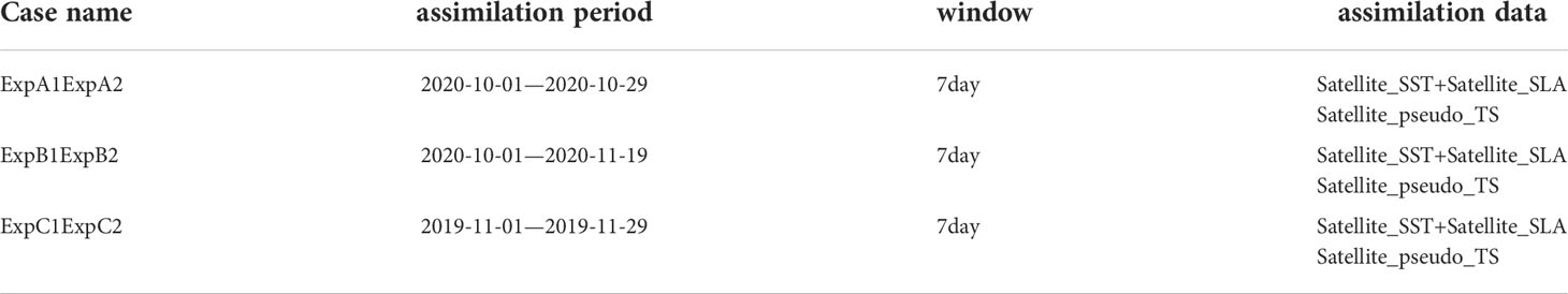
Table 2 Assimilation experiment setup.

In order to better visualize the effect of synthetic profiles assimilation on the improvement of the model underwater structure, we selected two area with mesoscale eddies for qualitative analysis. For regions with strong stratification, the selected area should not be too large, which could easily lead to inaccurate regression relationships between sea surface variables and underwater variables. Therefore, compared to the previous set of assimilation experiments, we reduced the selected area (Table 2). ExpB1 directly assimilated the satellite SST and SLA, and the adjustment of the underwater structure was carried out by model dynamical framework, while ExpB2 assimilated the synthetic T/S profiles based on SST and SLA. The period of this groups of experiments was from October 1, 2020 to November 19, 2020 with an assimilation window of 7 days. To more extensively verify the improvement effect of the machine learning-based assimilation system on the model underwater structure, another grid assimilation experiment was conducted. The period and the assimilation window are shown in Table 2. The assimilation data of ExpC1 and ExpC2 are the same as ExpB1 and ExpB2, respectively, but in different regions. To compare the assimilation effect, survey data for the Northwest Pacific were chosen as independent validation data for ExpBs and ExpCs. The measurement error of satellite observations for ExpB1 and ExpC1 is consistent with that of ExpA1 and the measurement error of synthetic profiles for ExpB2 and ExpC2 is shown in Table 1.

3 Evaluation of the accuracy of the synthetic profiles

Before assimilating the synthetic T/S profiles into the model, we evaluated the performance of the reconstruction model, including error analysis and characteristic analysis by comparing the synthetic profiles with the reanalysis product and the WOA13 climatology data.

3.1 Error analysis

To test the effectiveness of the synthetic model, the root mean square errors (RMSEs) of the 2019 synthetic T/S profiles, SODA3.4.2 reanalysis products, and WOA13 climatology data were calculated separately relative to the EN4.2.1 T/S profiles. The following equation was utilized to calculate the skill score of the synthetic profiles and SODA3.4.2 reanalysis product relative to the WOA13 climatology data (Zhu et al., 2022).

$\begin{array}{ll}Skill=1-\left(\frac{RMSE\left(m,o\right)}{RMSE\left(c,o\right)}\right)& (12)\end{array}$

where RMSE(m,o) represents the root mean square error between the target data and the EN4.2.1 in-situ data, and RMSE(c,o) stands for the root mean square error between the reference data and the EN4.2.1 in-situ data. We used the WOA13 climatology data as the reference data. When the RMSE of the target data was smaller than the RMSE of the reference data, the Skill was positive, and the closer it was to one, the greater the degree of improvement was.

The RMSE and the Skill of the synthetic T/S profiles are shown in Figure 3. In terms of temperature, the error distributions of the synthetic profiles and SODA3.4.2 reanalysis products are close and the depth averages of RMSE are basically equal (0.65 for SODA3.4.2 and 0.66 for the synthetic fields), indicating that the accuracy of the synthetic fields and the SODA3.4.2 product is comparable (Figure 3A). From the perspective of Skill, the synthetic temperature profiles show the advantage of accuracy in 150m-400m, while the accuracy of SODA3.4.2 reanalysis product is higher in the rest of the depths. The depth averages of Skill for the synthetic temperature profiles and the SODA3.4.2 reanalysis product are 0.34 and 0.36, respectively, which are almost equivalent (Figure 3C). From the perspective of salinity, the RMSE of the synthetic salinity profiles from 100 m to 300 m was similar to that of the WOA13 data but larger than that of the SODA3.4.2 product (Figure 3B). This is understandable since the 5 day-averaged SODA3.4.2 reanalysis product assimilates the satellite observations as well as the in-situ T/S profiles and the data used for comparison here belong to the in-situ T/S observations. In addition to the need to further enhance the accuracy near the thermocline layer, the accuracy of the synthetic salinity profiles was improved compared with the WOA13 data (Figure 3D).

FIGURE 3

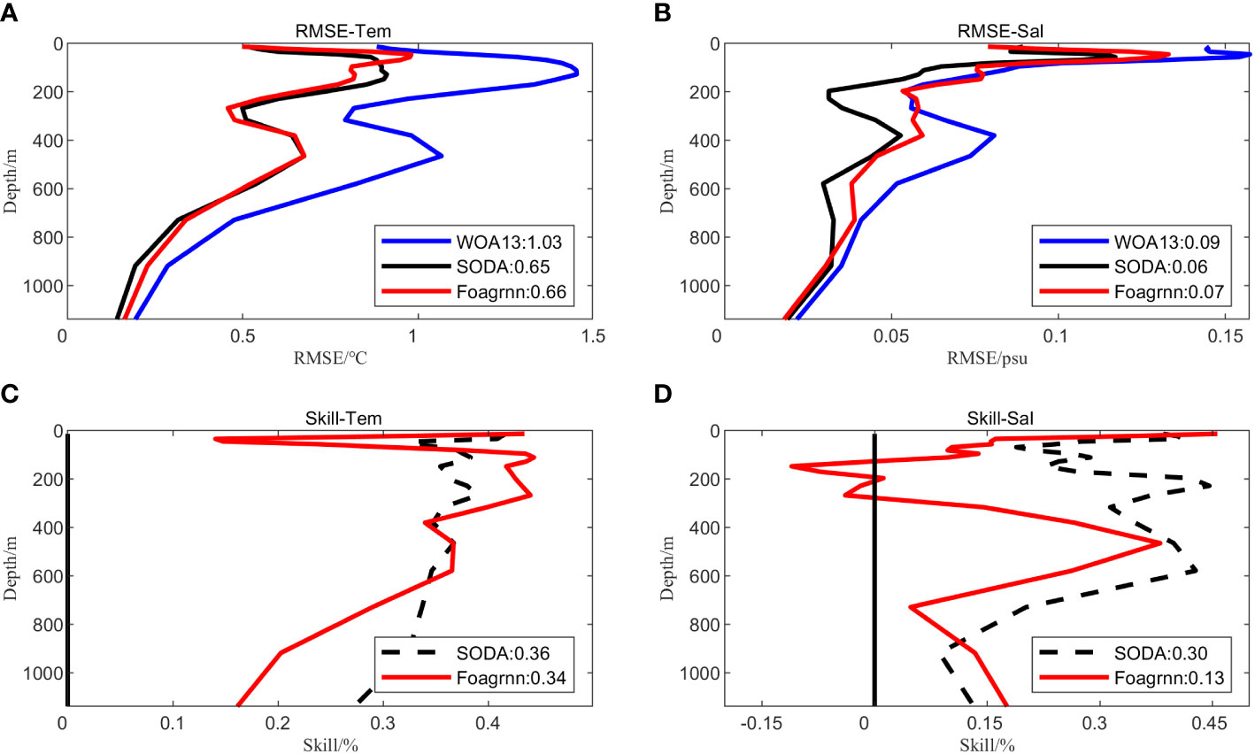
Figure 3 Temperature (left) and salinity (right) profiles root mean square errors (RMSEs) and skill scores as a function of depth. (A) temperature profiles RMSE, (B) salinity profiles RMSE, (C) skill score of temperature profiles relative to WOA13, (D) skill score of salinity profiles relative to WOA13. The black line represents SODA3.4.2 reanalysis data; the red line represents the synthetic profiles; the blue line represents WOA13 climatology data, and the numbers represent the depth mean of RMSE and skill score.

Figure 4 exhibits the horizontal distribution of RMSEs for the synthetic data and SODA3.4.2 reanalysis product relative to the EN4.2.1 in-situ profiles in 2019. Overall, the RMSE of synthetic temperature profiles was smaller than 1°C with a mean value of about 0.67°C, and the RMSE of the synthetic salinity profiles was smaller than 0.15 psu with a mean value of about 0.07 psu. There were 437 EN4.2.1 T/S profiles in 2019 and the RMSE of about 37% for the synthetic temperature profiles was smaller than that for the SODA3.4.2 temperature product, and the RMSE of about 30% for the synthetic salinity profiles was smaller than that for the SODA3.4.2 salinity product.

FIGURE 4

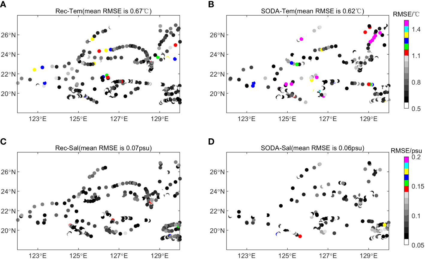
Figure 4 The distribution of RMSEs over space. Each row represents a different variable field. Each column represents a different data source: (A, C) the synthetic fields and (B, D) the SODA3.4.2 reanalysis data.

3.2 Characteristic analysis

We quantitatively analyzed the accuracy of the reconstructed model in Section 3.1. In this section, combined with the three-dimensional structural features of mesoscale eddies, we qualitatively analyze the reconstruction ability of the FOAGRNN method for the mesoscale eddy. Figure 5 depicts the distribution characteristics of SLA, sea surface temperature anomaly (SSTA), and sea surface salinity anomaly (SSSA). SSTA and SSSA are the anomalies of satellite data, synthetic fields, and GREP reanalysis product relative to WOA13 climatology data. The SLA for the synthetic data and GREP product is the anomaly of the vertically integrated dynamic height field relative to that calculated by WOA13 data. The synthetic profiles began at 10 m, thus, the SST and SSS of the synthetic data were approximately represented by the temperature and salinity values at this depth. It can be observed in Figure 5 that the characteristics (location and shape) of the mesoscale eddies calculated based on the synthetic temperature and salinity fields are closer to the observations than the results of the GREP product. One possible reason is that the reconstructed model incorporates much information from various surface observations. The changes with depth in the dynamic height anomaly field, temperature anomaly field, and salinity anomaly field are illustrated in Figure 6, respectively. The mesoscale eddies which were calculated by each element field of the synthetic data are quite consistent with the real sea surface eddies in both position and shape at these depth layers, indicating that the FOAGRNN algorithm has acceptable mesoscale eddy reconstruction capability.

FIGURE 5

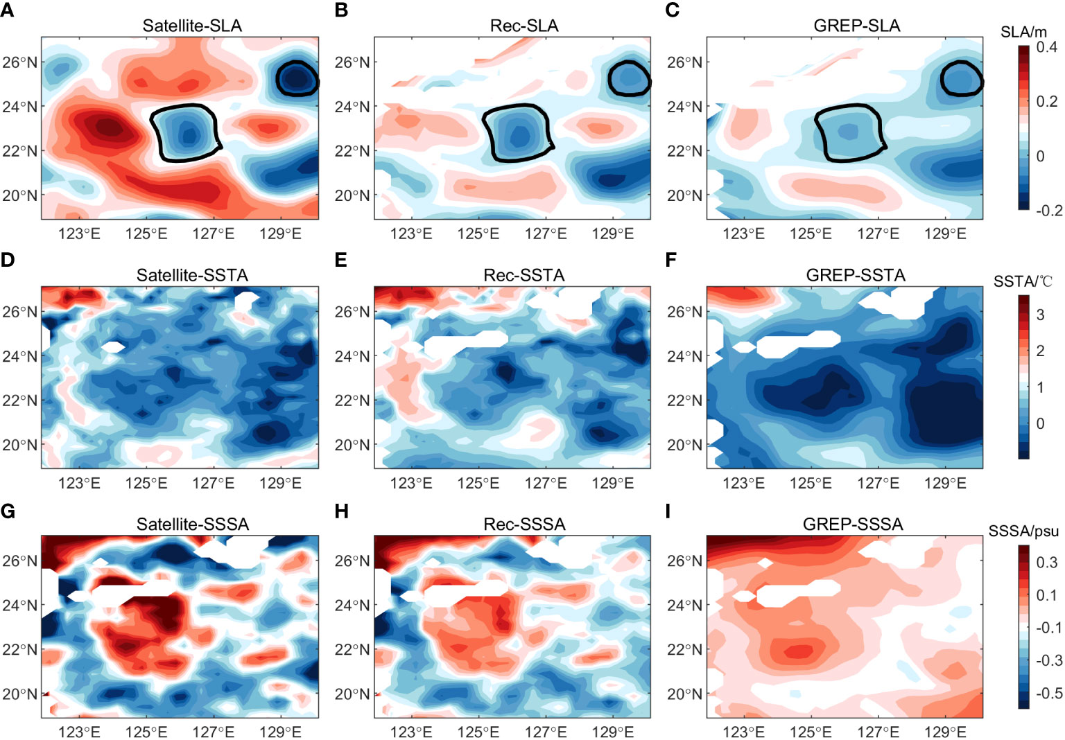
Figure 5 The distribution of the anomaly fields of sea surface level, temperature and salinity from satellite, synthetic fields and GREP reanalysis data on May 13, 2019. (A, D, G) the SLA, SSTA, and SSSA of the satellite observations, (B, E, H) the SLA, SSTA, and SSSA of the synthetic fields, (C, F, I) the SLA, SSTA, and SSSA of the GREP reanalysis product.

FIGURE 6

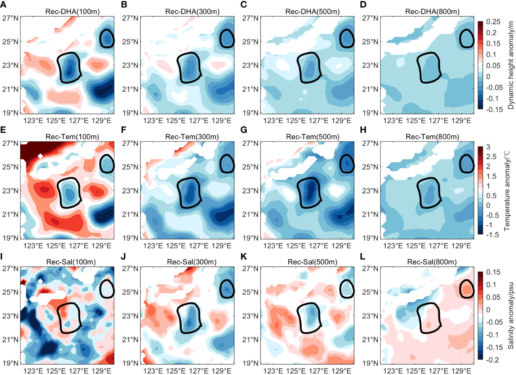
Figure 6 The distribution of the anomaly fields of dynamic height, temperature and salinity from the synthetic fields and on May 13, 2019. From left to right: 100m, 300m, 500m, and 800m. (A–D) the dynamic height anomaly fields of the synthetic fields, (E–H) the temperature anomaly fields of the synthetic fields, (I–L) the salinity anomaly fields of the synthetic fields. The circles in the figure are mesoscale eddies identified by satellite SLA.

4 Assimilation results of the synthetic T/S profiles

Through error analysis and characteristic analysis, section 3 suggested that the synthetic T/S profiles based on the machine learning method had sufficient accuracy. On this basis, we further conducted the following three groups of assimilation experiments.

4.1 Quantitative analysis

In order to make the RMSE statistically significant, we selected a relatively large area for the assimilation experiment. The RMSEs of the assimilation experiment results of each case relative to the EN4.2.1 in-situ T/S profiles are exhibited in Figure 7. In terms of temperature, ExpA1 has an error of more than 2°C at the thermocline, while ExpA2 has a reduced error at the 100-1100m depth layer. Compared to MODAS, ExpA2 shows higher accuracy at the thermocline and 300-800 m. The depth means of RMSE show that ExpA2 improves the simulation accuracy by 6.2% and 26.0% compared to MODAS and ExpA1, respectively (Figure 7A). From the perspective of salinity, compare with ExpA1, the experiment results of synthetic profiles not only reduce the error at the thermocline, but also have higher simulation accuracy at other depths with improvements in the simulation accuracy by 23.1%. The depth means of RMSE for ExpA2 and MODAS are basically equal (0.10 and 0.09, respectively), which shows that their simulation accuracy is comparable, and it may be related to both assimilating synthetic salinity profiles (Figure 7B).

FIGURE 7

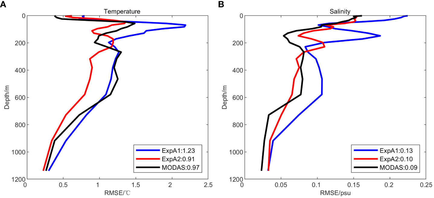
Figure 7 RMSEs of ROMS in nowcasting all the available EN4.2.1 T/S profiles. (A) temperature and (B) salinity (black line: MODAS data; red line: the experiment results of assimilating the synthetic T/S observations; blue line: the experiment results of assimilating sea surface observations). Numbers represent depth means of the RMSEs.

4.2 Qualitative analysis

4.2.1 Region one

The results of the error analysis show that the assimilation of synthetic profiles can improve the simulation accuracy of the model underwater structure compared to the direct assimilation of the satellite observations. In section 4.2, the impact of the synthetic profiles on the model underwater structure is assessed from the qualitative analysis. Figure 8 shows the temperature anomaly and salinity sections along the observation route. The temperature anomalies were obtained by subtracting the WOA13 climatology data from the in-situ survey data, MODAS data, and the experimental results of ExpB1 and ExpB2. In terms of temperature, the shape characteristics of ExpB1 were inconsistent with the in-situ section structure and the distribution of the temperature anomaly in the deep layer was also relatively higher than any other data. Both ExpB2 and MODAS data simulated a cold eddy structure similar to the in-situ one in the corresponding position, but the shape feature of ExpB2 was more consistent with the in-situ one (Figures 9A–D). From the perspective of salinity, compared with MODAS data and the experiment results of ExpB1, the salinity section structure of ExpB2 was more consistent with the in-situ measurements in terms of depth distribution and microstructure (Figures 9E–H).

FIGURE 8

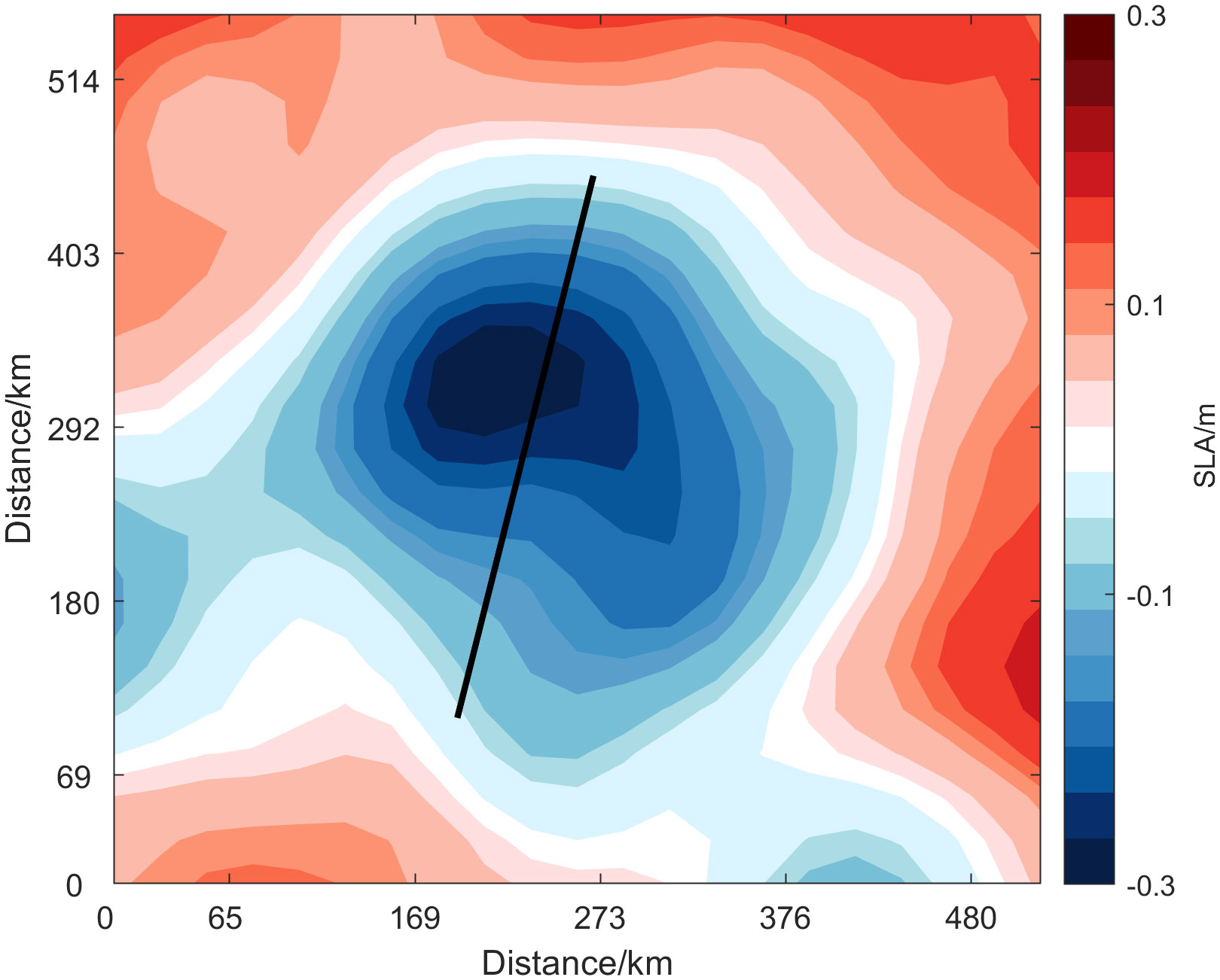
Figure 8 The distribution of the sea surface level anomalies on November 8, 2020 (unit: m). The black line represents the observation route of the Northwest Pacific survey data.

FIGURE 9

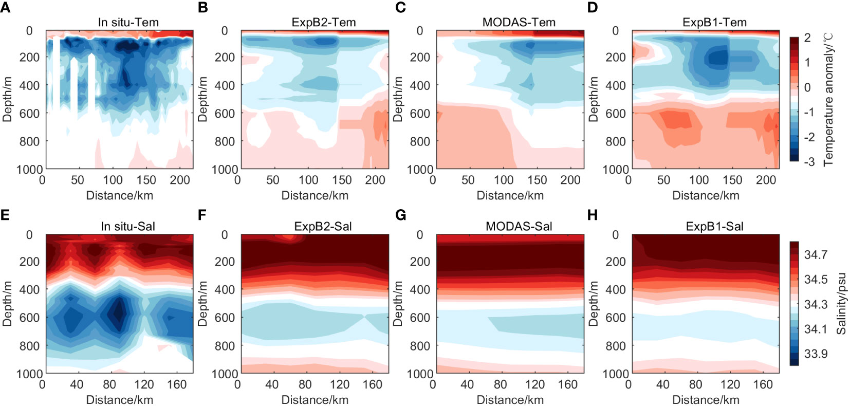
Figure 9 Temperature anomaly section and salinity section along the observation route. From top to bottom: temperature anomaly values and salinity values. (A, E) in-situ survey data, (B, F) the experiment results of assimilating the synthetic T/S observations, (C, G) the MODAS data of the National Marine Data Center, (D, H) the experiment results of assimilating the satellite observations. The abscissa represents the distance from the starting point of the survey data (unit: km).

4.2.2 Region two

The section where the red dots in Figure 10 are located was taken as the research section. Figures 11A–D reveal the temperature anomaly sections of the in-situ survey data, ExpC2, MODAS data, and ExpC1, respectively. Taking the depth of 200 m as the dividing line, an obvious dual-core structure can be observed in the in-situ temperature anomaly section structure. Compared with the assimilation results of ExpC1, both ExpC2 and MODAS data simulated a dual-core structure, but the strength of the cold eddy structure is not in line with the actual measurement. From the perspective of salinity anomaly sections, we can see in Figures 11E–H that there is a low-salinity center near 400 m in the in-situ salinity anomaly section. The salinity anomaly section structure of ExpC1 did not simulate a single-core structure in the deep layer, and the salinity anomaly value of ExpC1 near the sea surface was much larger than that of the in-situ survey data. The cold eddy structure could not be simulated by MODAS data, and the salinity anomalies at almost all depths were near 0 psu. This indicated that the salinity field of MODAS data was not much different from the WOA13 salinity background field. Differently, ExpC2 simulated an obvious single-core structure, but the depth range covered by the structure was larger than that by the in-situ salinity anomaly section.

FIGURE 10

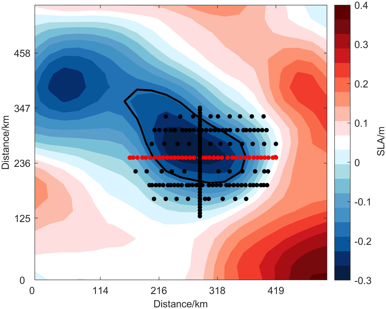
Figure 10 The distribution of survey stations of the Northwest Pacific cyclone eddy from November 13 to 15, 2019. The red dots represent the location of the study section, the color represents the sea surface level anomaly, and the circle in the figure is the mesoscale eddy identified by satellite SLA.

FIGURE 11

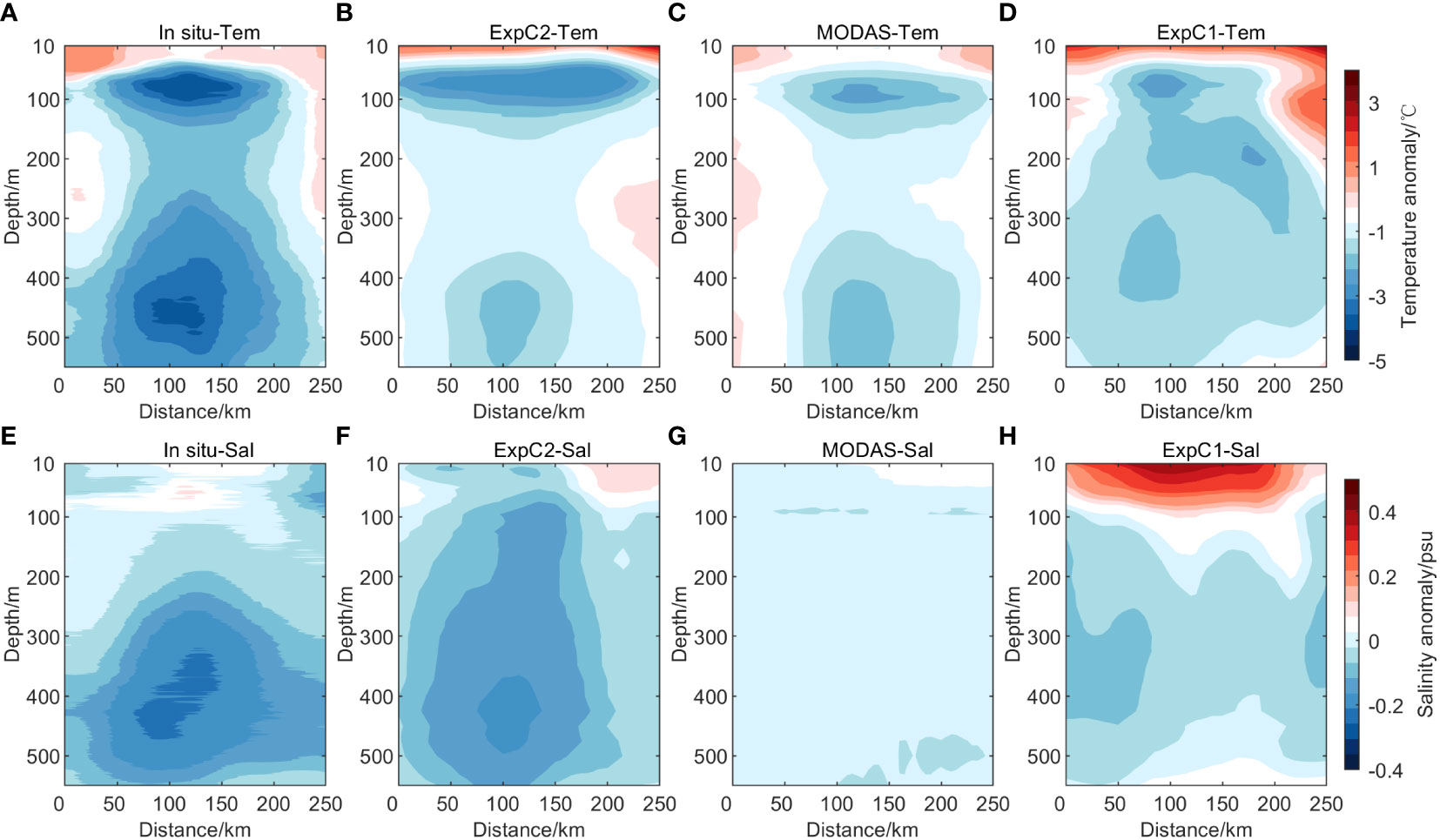
Figure 11 The section structure of the temperature and salinity anomaly at the position of the red dot in Figure 10. Top: temperature anomaly values; bottom: salinity anomaly values. (A, E) in-situ survey data, (B, F) the experiment results of assimilating the synthetic T/S observations, (C, G) the MODAS data of the National Marine Data Center, (D, H) the experiment results of assimilating the satellite observations.

Figure 12 illustrates the horizontal distribution of temperature and salinity anomaly at depths of 10 m, 100 m, 200 m, 300 m, 400 m, and 500 m. In terms of temperature anomaly, from 100m to 200m, the slice structure of ExpC1 was in good agreement with the in-situ data, suggesting that the direct assimilation of satellite data had a positive impact on the simulation of the model underwater structure at this depth layer. However, the cold eddy structure simulated by ExpC1 gradually disappeared in the subsequent depths. This indicated that the positive impact of the direct assimilation of satellite data was weakening with the change of depth, while MODAS data and ExpC2 could maintain the cold eddy structure with the change of depth (Figures 12A–D). From the perspective of salinity anomaly, ExpC1 could not simulate the cold eddy structure, and similar to Figure 11G, the salinity anomalies of MODAS data at all depths were around zero, indicating that MODAS salinity data were almost the same as WOA13 climatology salinity data. ExpC2 simulated both the cold eddy structure and the intensity variation trend close to the in-situ measurement (Figures 12E–H).

FIGURE 12

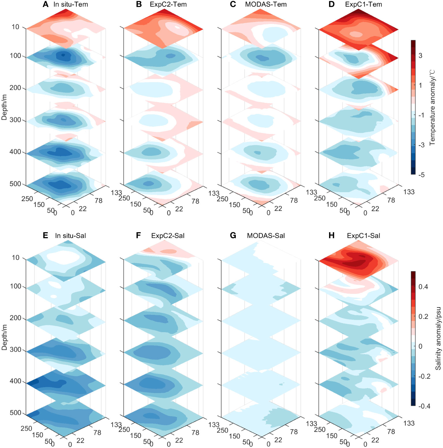
Figure 12 Temperature and salinity anomaly slices at 10m, 100m, 200m, 300m, 400m, and 500m. (A, E) the in-situ data, (B, F) the experiment results of assimilating the synthetic T/S profiles, (C, G) the MODAS data of the National Marine Data Center, and (D, H) the experiment results of the direct assimilation of satellite observations. The unit of abscissa and ordinate is km.

5 Conclusion and discussion

Satellite data are very important for marine operational forecasting systems, however, the traditional method of the direct assimilation of satellite observations cannot constrain the simulation of underwater structures well. To address this problem, we created a machine learning-based assimilation system. First, the historical EN4.2.1 in-situ T/S profiles and historical satellite altimeter data were employed as the training data of the FOAGRNN to construct a reconstruction model. Then satellite observations (SST, SLA, SSS) were utilized as the input data of the reconstruction model to reconstruct three-dimensional T/S pseudo-profiles. Finally, the I4D-Var method was used to assimilate the synthetic data into the ROMS, and three groups of assimilation experiments were performed. A validation of the synthetic T/S profiles and the assimilation experiments results against the observations indicates that

1. In addition to the need to further enhance the accuracy near the thermocline, the accuracy of the synthetic profiles is comparable to the 5-day averaged SODA 3.4.2 reanalysis product and better than the WOA13 climatology data. The horizontal distribution of RMSE shows that the error of the synthetic temperature profiles is within 1°C, while the error for salinity is within 0.15 psu. The profiles with better quality than the SODA3.4.2 reanalysis product occupy an acceptable proportion in total. A validation against the GREP reanalysis products shows that the synthetic fields have better mesoscale eddy reconstruction ability. Moreover, the mesoscale eddies which were calculated by each element field of the synthetic data are quite consistent with the real sea surface eddies in both position and shape at the selected depths.

2. A validation against the EN4.2.1 in-situ T/S profiles (with 107 observed profiles) shows that compared with direct assimilation of satellite remote sensing observations, the simulation accuracy of assimilating synthetic profiles shows a significant improvement at the thermocline, with a 26.0% reduction for temperature and a 23.1% reduction for salinity in RMSE. Compared with MODAS, the simulation accuracy of assimilating synthetic profiles is improved by 6.2% in temperature and comparable in salinity.

3. Survey data from the Northwest Pacific were used as independent observations for the qualitative analysis of the assimilation effect, which demonstrates that compared with the direct assimilation of satellite remote sensing observations, the indirect assimilation based on machine learning can significantly improve the simulation effect of model underwater structure, and compared with MODAS, the machine learning-based assimilation system demonstrated a significant advantage in the simulation of underwater salinity structure.

Compared with the direct assimilation of satellite observations, the indirect assimilation based on the machine learning substantially improved the simulation effect of model underwater structures, which can provide a more accurate initial condition for ocean models to more accurately predict ocean phenomena, such as mesoscale eddies. Moreover, as an application example, our study can promote more scholars to explore the combination of machine learning and data assimilation in different ways, especially for applications of satellite data in the operational system. However, there is still a lot of optimization work to be done in the future.

1. There are mainly two error sources in the salinity profile estimation. First, the satellite SSS data still have various types of errors from the instrument’s observations, brightness temperature Tb reconstruction, and salinity retrieval algorithm, especially at high latitudes. Second, the training data of the reconstruction model were based on years of in-situ T/S profiles, while the input data used to construct the real-time T/S pseudo-profiles originated from satellite observations. Different depth distributions of salinity values will inevitably cause errors in the synthetic profiles. Therefore, the following study can attempt to directly use the satellite observations as training data or to describe the characteristic of the relationship between in-situ SSS and satellite SSS.

2. when the machine learning algorithm reconstructs the T/S profiles in a complex stratified region, such as mesoscale eddies, the region of the selected sample data should be limited to a certain range. Otherwise, the empirical relationship between surface observations and underwater variable fields may not be representative, and the error of the synthetic profiles may be large. However, if the range is too small, the number of the in-situ T/S profiles in the study area will be scarce, and an effective reconstruction model may not be constructed. To compensate for this deficiency, it is possible to employ reanalysis products as training data to build a reconstruction model since the reanalysis data of each current platform have good simulation accuracy, which can provide favorable preconditions for the realization of this goal (Compo et al., 2011; Dee et al., 2011).

3. In terms of the assimilation, this study assumed that the observation errors were uncorrelated in time and space and prescribed a single scalar for all synthetic observations, which simplified the construction of the observation error covariance matrix, but in fact, the synthetic T/S profiles had a certain correlation, and a single scalar for all synthetic observations may cause under/overestimation of synthetic observations in the wrong places. Moreover, a large number of synthetic T/S profiles, which were not sparse enough, likely affected the assimilation efficiency.

Data availability statement

The raw data supporting the conclusions of this article will be made available by the authors, without undue reservation.

Author contributions

Data curation, ZC, PW, and SB. Visualization, ZC and PW. Software, ZC, PW, and SB. Writing – original draft, ZC. Review of the manuscript, PW, SB, and WZ. Funding, WZ. All authors have read and agreed to the published version of the manuscript.

Funding

This paper is supported by the National Key R&D Plan Project, Regional Multi-layer Coupling Data Assimilation (2021YFC3101500).

Conflict of interest

The authors declare that the research was conducted in the absence of any commercial or financial relationships that could be construed as a potential conflict of interest.

Publisher’s note

All claims expressed in this article are solely those of the authors and do not necessarily represent those of their affiliated organizations, or those of the publisher, the editors and the reviewers. Any product that may be evaluated in this article, or claim that may be made by its manufacturer, is not guaranteed or endorsed by the publisher.

References

Bao S., Zhang R., Wang H., Yan H., Yu Y., Chen J. (2019). Salinity profile estimation in the pacific ocean from satellite surface salinity observations. J. Atmospheric Oceanic Technol. 36 (1), 53–68. doi: 10.1175/jtech-d-17-0226.1

CrossRef Full Text | Google Scholar

Carnes M. R., Teague W. J., Mitchell J. L. (1994). Inference of subsurface thermohaline structure from fields measurable by satellite. J. Atmospheric Oceanic Technol. 11 (2), 551–566. doi: 10.1175/1520-0426(1994)011<0551:Iostsf>2.0.Co;2

CrossRef Full Text | Google Scholar

Carton J. A., Chepurin G. A., Chen L. (2018). SODA3: A new ocean climate reanalysis. J. Climate 31 (17), 6967–6983. doi: 10.1175/jcli-d-18-0149.1

CrossRef Full Text | Google Scholar

Chapman C., Charantonis A. A. (2017). Reconstruction of subsurface velocities from satellite observations using iterative self-organizing maps. IEEE Geosci. Remote Sens. Lett. 14 (5), 617–620. doi: 10.1109/LGRS.2017.2665603

CrossRef Full Text | Google Scholar

Chen K., He R., Powell B. S., Gawarkiewicz G. G., Moore A. M., Arango H. G. (2014). Data assimilative modeling investigation of gulf stream warm core ring interaction with continental shelf and slope circulation. J. Geophysical Research: Oceans 119 (9), 5968–5991. doi: 10.1002/2014JC009898

CrossRef Full Text | Google Scholar

Chen X., Wang H., Zheng F., Cai Q. (2020). An ensemble-based SST nudging method proposed for correcting the subsurface temperature field in climate model. Acta Oceanologica Sin. 39 (3), 73–80. doi: 10.1007/s13131-020-1568-2

CrossRef Full Text | Google Scholar

Chen Y., Yan C., Zhu J. (2018). Assimilation of Sea surface temperature in a global hybrid coordinate ocean model. Adv. Atmospheric Sci. 35 (10), 1291–1304. doi: 10.1007/s00376-018-7284-6

CrossRef Full Text | Google Scholar

Compo G. P., Whitaker J. S., Sardeshmukh P. D., Matsui N., Allan R. J., Yin X., et al. (2011). The twentieth century reanalysis project. Q. J. R. Meteorological Soc. 137 (654), 1–28. doi: 10.1002/qj.776

CrossRef Full Text | Google Scholar

Cooper M., Haines K. (1996). ). altimetric assimilation with water property conservation. J. Geophysical Research: Oceans 101 (C1), 1059–1077. doi: 10.1029/95JC02902

CrossRef Full Text | Google Scholar

Cummings J. A., Smedstad O. M. (2013). ““Variational data assimilation for the global ocean,”,” in Data assimilation for atmospheric, oceanic and hydrologic applications (Vol. II). Eds. Park S. K., Xu L. (Berlin, Heidelberg: Springer Berlin Heidelberg), 303–343.

Google Scholar

Dai J., Wang H., Zhang W., Wang P., Luo T. (2021). Three-dimensional structure of an observed cyclonic mesoscale eddy in the Northwest pacific and its assimilation experiment. Acta Oceanologica Sin. 40 (5), 1–19. doi: 10.1007/s13131-021-1810-6

CrossRef Full Text | Google Scholar

Dee D. P., Uppala S. M., Simmons A. J., Berrisford P., Poli P., Kobayashi S., et al. (2011). The ERA-interim reanalysis: configuration and performance of the data assimilation system. Q. J. R. Meteorological Soc. 137 (656), 553–597. doi: 10.1002/qj.828

CrossRef Full Text | Google Scholar

Ezer T., Mellor G. L. (1994). Continuous assimilation of geosat altimeter data into a three-dimensional primitive equation gulf stream model. J. Phys. Oceanography 24 (4), 832–847. doi: 10.1175/1520-0485(1994)024<0832:Caogad>2.0.Co;2

CrossRef Full Text | Google Scholar

Fox D. N., Teague W. J., Barron C. N., Carnes M. R., Lee C. M. (2002). The modular ocean data assimilation system (MODAS). J. Atmospheric Oceanic Technol. 19 (2), 240–252. doi: 10.1175/1520-0426(2002)019<0240:Tmodas>2.0.Co;2

CrossRef Full Text | Google Scholar

Good S., Fiedler E., Mao C., Martin M. J., Maycock A., Reid R., et al. (2020). The current configuration of the OSTIA system for operational production of foundation Sea surface temperature and ice concentration analyses. Remote Sens. 12 (4), 720. doi: 10.3390/rs12040720

CrossRef Full Text | Google Scholar

Good S. A., Martin M. J., Rayner N. A. (2013). EN4: Quality controlled ocean temperature and salinity profiles and monthly objective analyses with uncertainty estimates. J. Geophysical Research: Oceans 118 (12), 6704–6716. doi: 10.1002/2013JC009067

CrossRef Full Text | Google Scholar

Haines K. (1991). A direct method for assimilating Sea surface height data into ocean models with adjustments to the deep circulation. J. Phys. Oceanography 21 (6), 843–868. doi: 10.1175/1520-0485(1991)021<0843:Admfas>2.0.Co;2

CrossRef Full Text | Google Scholar

Helber R. W., Townsend T. L., Barron C. N., Dastugue J. M., Carnes M. R. (2013). “Validation test report for the improved synthetic ocean profile (ISOP) system, part I: Synthetic profile methods and algorithm” (Naval Research Lab Stennis Detachment Stennis Space Center Ms Oceanography Div).

Google Scholar

He Z., Wang X., Wu X., Chen Z., Chen J. (2021). Projecting three-dimensional ocean thermohaline structure in the north Indian ocean from the satellite Sea surface data based on a variational method. J. Geophysical Research: Oceans 126 (1), e2020JC016759. doi: 10.1029/2020JC016759

CrossRef Full Text | Google Scholar

Holland W. R., Malanotte-Rizzoli P. (1989). Assimilation of altimeter data into an ocean circulation model: Space versus time resolution studies. J. Phys. Oceanography 19 (10), 1507–1534. doi: 10.1175/1520-0485(1989)019<1507:Aoadia>2.0.Co;2

CrossRef Full Text | Google Scholar

Iqbal Z., Shahid S., Ahmed K., Wang X., Ismail T., Gabriel H. F. (2022). Bias correction method of high-resolution satellite-based precipitation product for peninsular Malaysia. Theor. Appl. Climatology 148 (3), 1429–1446. doi: 10.1007/s00704-022-04007-6

CrossRef Full Text | Google Scholar

Le X.-H., Lee G., Jung K., An H.-u., Lee S., Jung Y. (2020). Application of convolutional neural network for spatiotemporal bias correction of daily satellite-based precipitation. Remote Sens. 12 (17), 2731. doi: 10.3390/rs12172731

CrossRef Full Text | Google Scholar

Li H.-z., Guo S., Li C.-j., Sun J.-q. (2013). A hybrid annual power load forecasting model based on generalized regression neural network with fruit fly optimization algorithm. Knowledge-Based Syst. 37, 378–387. doi: 10.1016/j.knosys.2012.08.015

CrossRef Full Text | Google Scholar

Lin S.-M. (2013). Analysis of service satisfaction in web auction logistics service using a combination of fruit fly optimization algorithm and general regression neural network. Neural Computing Appl. 22 (3), 783–791. doi: 10.1007/s00521-011-0769-1

CrossRef Full Text | Google Scholar

Liu L., Xue H., Sasaki H. (2019). Reconstructing the ocean interior from high-resolution Sea surface information. J. Phys. Oceanography 49 (12), 3245–3262. doi: 10.1175/jpo-d-19-0118.1

CrossRef Full Text | Google Scholar

Liu L., Xue H., Sasaki H. (2021). Diagnosing subsurface vertical velocities from high-resolution Sea surface fields. J. Phys. Oceanography 51 (5), 1353–1373. doi: 10.1175/jpo-d-20-0152.1

CrossRef Full Text | Google Scholar

Moore A. M., Arango H. G., Broquet G., Edwards C., Veneziani M., Powell B., et al. (2011a). The regional ocean modeling system (ROMS) 4-dimensional variational data assimilation systems: Part II – performance and application to the California current system. Prog. Oceanography 91 (1), 50–73. doi: 10.1016/j.pocean.2011.05.003

CrossRef Full Text | Google Scholar

Moore A. M., Arango H. G., Broquet G., Powell B. S., Weaver A. T., Zavala-Garay J. (2011b). The regional ocean modeling system (ROMS) 4-dimensional variational data assimilation systems: Part I – system overview and formulation. Prog. Oceanography 91 (1), 34–49. doi: 10.1016/j.pocean.2011.05.004

CrossRef Full Text | Google Scholar

Ratheesh S., Sharma R., Basu S. (2012). Projection-based assimilation of satellite-derived surface data in an Indian ocean circulation model. Mar. Geodesy 35 (2), 175–187. doi: 10.1080/01490419.2011.637855

CrossRef Full Text | Google Scholar

Storto A., Masina S., Simoncelli S., Iovino D., Cipollone A., Drevillon M., et al. (2019). The added value of the multi-system spread information for ocean heat content and steric sea level investigations in the CMEMS GREP ensemble reanalysis product. Climate dynamics 53 (1), 287–312. doi: 10.1007/s00382-018-4585-5

CrossRef Full Text | Google Scholar

Su H., Li W., Yan X.-H. (2018). Retrieving temperature anomaly in the global subsurface and deeper ocean from satellite observations. J. Geophysical Research: Oceans 123 (1), 399–410. doi: 10.1002/2017JC013631

CrossRef Full Text | Google Scholar

Su H., Wu X., Yan X.-H., Kidwell A. (2015). Estimation of subsurface temperature anomaly in the Indian ocean during recent global surface warming hiatus from satellite measurements: A support vector machine approach. Remote Sens. Environ. 160, 63–71. doi: 10.1016/j.rse.2015.01.001

CrossRef Full Text | Google Scholar

Tranchant B., Remy E., Greiner E., Legalloudec O. (2019). Data assimilation of soil moisture and ocean salinity (SMOS) observations into the Mercator ocean operational system: focus on the El niño 2015 event. Ocean Sci. 15 (3), 543–563. doi: 10.5194/os-15-543-2019

CrossRef Full Text | Google Scholar

Vernieres G., Kovach R., Keppenne C., Akella S., Brucker L., Dinnat E. (2014). The impact of the assimilation of aquarius sea surface salinity data in the GEOS ocean data assimilation system. J. Geophysical Research: Oceans 119 (10), 6974–6987. doi: 10.1002/2014JC010006

CrossRef Full Text | Google Scholar

Wang P., Zhu M., Chen Y., Zhang W., Yu Y. (2021). Ocean satellite data assimilation using the implicit equal-weights variational particle smoother. Ocean Model. 164, 101833. doi: 10.1016/j.ocemod.2021.101833

CrossRef Full Text | Google Scholar

Weaver A. T., Deltel C., Machu E., Ricci S., Daget N. (2005). A multivariate balance operator for variational ocean data assimilation. Q. J. R. Meteorological Soc. 131 (613), 3605–3625. doi: 10.1256/qj.05.119

CrossRef Full Text | Google Scholar

Zhang W. G., Wilkin J. L., Arango H. G. (2010). Towards an integrated observation and modeling system in the new York bight using variational methods. part I: 4DVAR data assimilation. Ocean Model. 35 (3), 119–133. doi: 10.1016/j.ocemod.2010.08.003

CrossRef Full Text | Google Scholar

Zhou W., Li J., Xu F., Shu Y., Feng Y. (2021). The impact of ocean data assimilation on seasonal predictions based on the national climate center climate system model. Acta Oceanologica Sin. 40 (5), 58–70. doi: 10.1007/s13131-021-1732-3

CrossRef Full Text | Google Scholar

Zhu X., Zu Z., Ren S., Zhang M., Zhang Y., Wang H., et al. (2022). Improvements in the regional south China Sea operational oceanography forecasting system (SCSOFSv2). Geosci. Model. Dev. 15 (3), 995–1015. doi: 10.5194/gmd-15-995-2022

CrossRef Full Text | Google Scholar