Dynamic analysis of an axially moving underwater pipe conveying pulsating fluid

In this paper, both linear and non-linear dynamics of a slender and uniform pipe conveying pulsating fluid, which is axially moving in an incompressible fluid, are comprehensively studied. The vibration equations of the system are established by considering various factors, including a coordinate conversion system, an “axial added mass coefficient” describing the additional inertia forces caused by the external fluid, the Kelvin–Voigt viscoelastic damping, a kind of non-linear additional axial tension, and the pulsating internal fluid. The vibration equations are discretized by the Galerkin procedure and solved by the Runge–Kutta approach, and the validity of the solution procedure is carefully checked. After that, the linear and non-linear responses of the system are studied when the internal flow velocity and the axially moving speed of the pipe are small. For linear responses, the Kelvin–Voigt viscoelastic damping has great influences on the second and third modes of the system. For the non-linear dynamic, the results are rich and changeful, including the first and second principal parametric resonances, the secondary resonance, the combination resonance, period-1 motion, quasi-periodic motion, and chaotic motion. Finally, the influence of several key system parameters on the non-linear responses is analyzed.

1 Introduction

The linear and non-linear dynamics of a pipe conveying fluid have been widely researched decades before. Paїdoussis (Païdoussis and Li, 1993; Païdoussis, 1998; Païdoussis, 2003) made extensive reviews about the early works on these subjects. These reviews discussed various aspects on the dynamics of the pipe conveying fluid, such as mathematical modeling, solution methodology, the mechanisms of instabilities, and the linear and non-linear and chaotic dynamics. In these reviews, the impact of various parameters on the system dynamics is also discussed, such as boundary conditions, steady or unsteady internal flow, fluid friction effects, elastic constraints or motion-limiting constraints, and elastic foundation. Paїdoussis pointed out that, although the model of the pipe conveying fluid was simple, the motion equation of it contained not only the general dynamic characteristics of the bar and beam system but also gyroscopic force caused by the internal fluid, so that the pipe conveying fluid revealed more extensive dynamic behaviors and became a new paradigm to study fluid–structure interactions that refer to slender structures and axial flows.

In some cases, the in-pipe flow velocity may contain harmonic components, i.e., pulsating fluid, and the harmonic components may lead to parametric instability. In the early research studies, notably done by Ginsberg, 1973 and Païdoussis and Issid (1974), linearized analytical models and numerical methods were adopted to reveal the parametric instability of simply supported straight pipes. In the subsequent research studies, various non-linear models were introduced to further study the system under different kinds of parametric resonance, notably by Namachchivaya and Tien (Namachchivaya, 1989; Namachchivaya and Tien, 1989a; Namachchivaya and Tien, 1989b), Jayaraman and Narayanan (1996), Öz (Öz and Boyaci, 2000; Öz et al., 2001), Jin and Song (2005), Panda and Kar (Panda and Kar, 2007; Panda and Kar, 2008), Wang (Wang, 2009; Wang, 2010), and Ni et al. (2014). These works showed that a pipe conveying pulsating fluid performed abundant non-linear dynamical phenomena.

In the above studies, the pipe systems were fixed. However, in some engineering devices, the systems may have axial movement, such as robotic systems, underwater towed cables, and conveyor belts. The axial movement of these systems can significantly impact on the transverse vibration of the systems. Hence, the dynamic behaviors of axially moving flexible bodies had been widely studied. Notable contributions in these works were by Balakrishnan (1985); Kane et al., 1987; Du et al., 1992; Shabana, 1997; Hyun and Yoo, 1999; Liu et al., 2007; Yoo et al., 2009 and Gerstmayr (2013).

If an axially moving structure is surrounded by fluid, then the influences of the external fluid cannot be ignored. For example, in the aircraft in-flight refueling process, after the refueling pipeline is connected, the refueling plane and the receiving plane keep at a static flight state relative to each other. In this case, the surrounding air will have an axial relative velocity to the pipeline, which will affect the stability of the pipeline. The underwater towing slender structure is another typical example. Dynamics and stability of an underwater axially extending cantilever beam are first studied by Taleb and Misra (2012). However, in the recent work, – provided a more accurate model, containing an “axial added mass coefficient”, for better calculating the external fluid dynamic forces. After that, the dynamic behaviors of an axially moving underwater beam constrained by torsion springs are investigated by Wang and Ni (2008). Most recently, Ni and Li (Ni and Li, 2014; Li et al., 2015) studied the dynamic behaviors of an underwater moving beam with different boundary conditions. Dynamics of an axially moving and extending cantilever beam as well as a sliding pipe conveying fluid are intensively studied by Yan (Yan et al., 2016; Yan et al., 2018; Yan et al., 2020). Huo and Wang (2016) studied the dynamic behaviors of a vertically stretching cantilevered pipe with internal fluid but without external fluid. In the author’s previous research, linear dynamics of an axially moving underwater pipe conveying fluid are analyzed (Ni et al., 2017). In the latest research, Zhou and Dai (Zhou et al., 2022) designed an underwater bio-inspired robot based on a cantilevered pipe, as shown in Figure 1. By changing the velocity of the internal fluid of the pipe, the vibration response of the pipe can be adjusted to control the movement of the robot. In summary, the axially moving pipe structure has a wide range of applications in engineering, especially in the control of the underwater moving structure. However, there are few studies on these structures, and existing research studies mainly focus on the linear dynamics. The non-linear dynamics of these structures, especially the non-linear dynamics under internal pulsating fluid, need to be further studied.

FIGURE 1

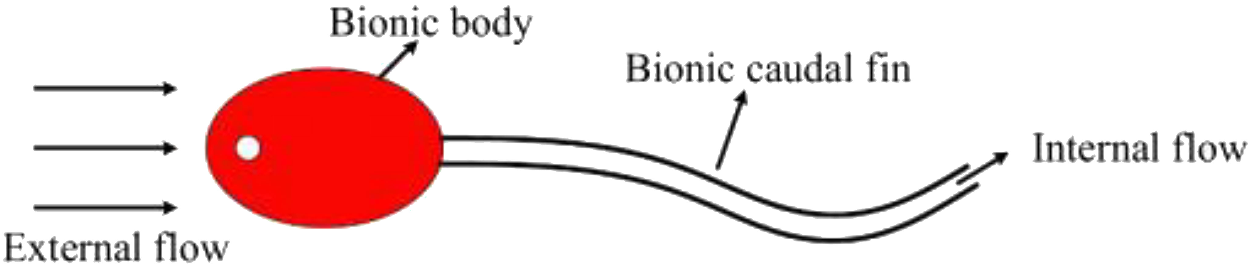
Figure 1 The underwater bio-inspired robot designed by Zhou and Dai (Zhou et al., 2022).

In this paper, both linear and non-linear dynamic behaviors of a slender and uniform pipe conveying pulsating fluid, which is axially moving in an incompressible fluid, are comprehensively studied. The content of this paper is arranged as follows. In Section 2, the vibration equations of the system are established by considering various factors. In Section 3, the vibration equations are discretized by the Galerkin procedure and solved by the Runge–Kutta approach. In Section 4, the validity of the solution procedure is carefully checked. In Section 5, the linear and non-linear responses of the system are studied as follows: First, the linear dynamic of the pipe system are studied; second, the non-linear dynamic responses are studied considering the non-linear additional pipe axial force while the pulsating component of the internal flow is neglected; third, the non-linear dynamic responses of the system under pulsating internal flow are investigated; last, the influence of several key system parameters on the non-linear responses is analyzed. The parameter instability region diagram of the system is obtained according to the Floquet theory. Furthermore, some typical system motions are identified by the bifurcation diagram, time history curve, power spectral density (PSD), phase trajectory, and Poincaré map. The conclusions are shown in Section 6.

2 Systematic formulation and theoretical derivation

The analysis system is shown in Figure 2. Consider a uniform simply supported pipe of outer diameter D, length l, internal perimeter S, mass per unit length m_p, flexural rigidity EI, internal cross-sectional area A_i, and conveying fluid of mass per unit length m_f, with axial flow velocity V relative to the pipe, the fluid pressure p_i. The pipe is axially moving at a speed L(t). The whole system is surrounded by incompressible fluid of density ρ, and the effect of the boundaries can be neglected. In the present study, it is further assumed that there no separation occurs in the cross-flow, and the fluid forces acting on a pipe element are the same as those acting on a corresponding element of a long undeformed pipe of the same cross-sectional area and inclination.

FIGURE 2

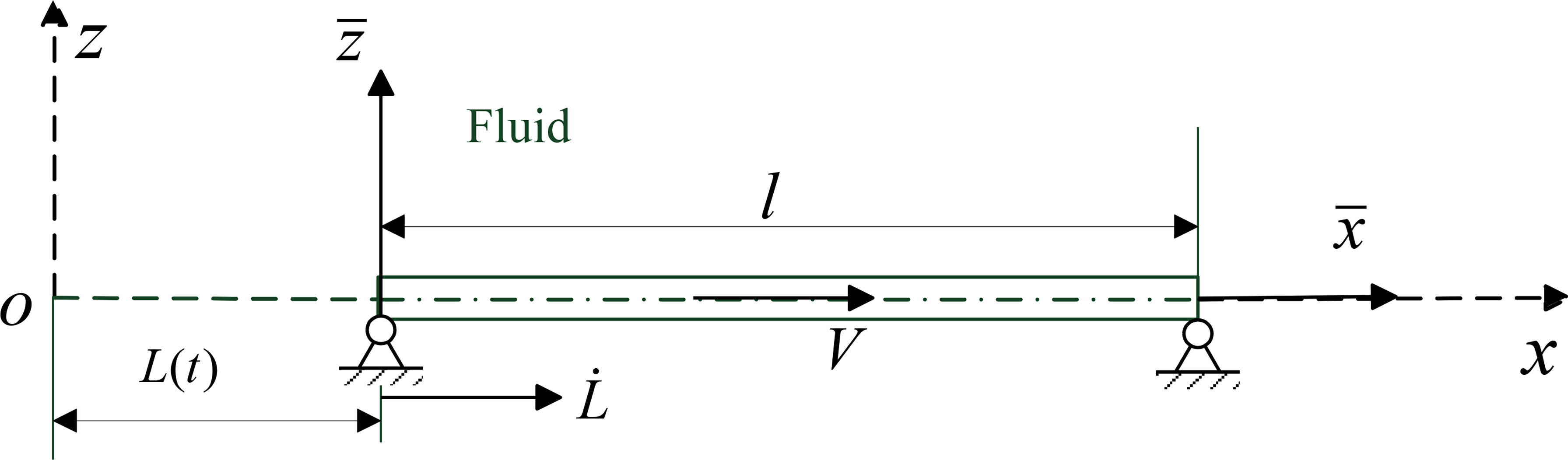
Figure 2 The analysis system and the corresponding coordinates.

For better description of the motion of the pipe system, two coordinate frames are set up on the basis of the previous studies (Ni and Li, 2014; Li et al., 2015): the absolute coordinate frame (x,z) and the moving coordinate frame $(\overline{x},\overline{z})$ relative to the supports. In the absolute coordinate frame (x,z), the motions of the pipe can be separated into two parts: axial displacement v(x,t) and the transverse displacement w(x,t). The axial displacement of the pipe includes the axial deformation and the axial motion. The axial deformation of the pipe is quite small compared to the transverse displacement and can be neglected, so the axial displacement of the pipe can be expressed as:

$\begin{array}{ll}v=v_{translation}=L(t)& (1)\end{array}$

The moving coordinate frame is defined as:

$\begin{array}{ll}\overline{x}=x-L(t);\overline{z}=z;\overline{t}=t& (2)\end{array}$

In addition, the relationship of derivative between two coordinates is expressed as:

$\begin{array}{ll}\{\begin{array}{l}\frac{\partial }{\partial x}=\frac{\partial }{\partial \overline{x}},\hfill \\ \frac{\partial }{\partial t}=\frac{\partial }{\partial \overline{t}}+\frac{\partial }{\partial \overline{x}}\frac{\partial \overline{x}}{\partial t}=\frac{\partial }{\partial \overline{t}}-\dot{L}\frac{\partial }{\partial \overline{x}}=\frac{\partial }{\partial \overline{t}}-\dot{L}\frac{\partial }{\partial x}\hfill \end{array}& (3)\end{array}$

Utilizing the Newton approach and the relationship of derivative between two coordinates, the equations of motion in the moving coordinate have been obtained in the previous work [Equation (32) in the work by Ni and Luo (Ni et al., 2017), and details of the derivation can also be found in it]:

$\begin{array}{ll}\begin{array}{c}EI\frac{{\partial }^{4}w}{\partial {\overline{x}}^4}\{m_f{V}^2+M[(\beta -1)\dot{L}{]}^2-T_l+[m_f\dot{V}+(m_f+m_p+\beta M)\ddot{L}+\frac{1}{2}{C}_T\left(\frac{M}{D}\right){\dot{L}}^2+\frac{\partial p_o}{\partial \overline{x}}{A}_o](l-\overline{x})\}\frac{{\partial }^{2}w}{\partial {\overline{x}}^2}-\\ \left[\frac{\partial p_o}{\partial \overline{x}}{A}_o+(m_f+m_p+M)\ddot{L}\right]\frac{\partial w}{\partial \overline{x}}+2[m_{f}V+M(\beta -1)\dot{L}]\frac{{\partial }^{2}w}{\partial \overline{x}\partial \overline{t}}+\\ \frac{1}{2}\left(\frac{M}{D}\right)(\dot{L}{C}_N+{\tilde{C}}_N)\frac{\partial w}{\partial \overline{t}}+(m_f+m_p+M)\frac{{\partial }^{2}w}{\partial {\overline{t}}^2}=0\end{array}& (4)\end{array}$

where p_o and A_o are the hydrostatic pressure and the area of the cross-section of the beam; T_l is the linear axial tension; M is the lateral direction virtual mass per unit length; β is an “axially added mass coefficient” presented by Gosselin et al. (2007); and C_N, ${\tilde{C}}_N$ and C_T can be derived from the normal and tangential drag coefficients by Taylor (1952).

When the direction of gravity and the x-axis are orthogonal, the gradient of the external pressure along the x-direction can be neglected, namely,

$\begin{array}{ll}\frac{\partial p_o}{\partial x}=0& (5)\end{array}$

In this paper, the internal dissipation model of the Kelvin–Voigt type is introduced to improve the equations of motion. By introducing Equation (5), the equations of motion [Equation (4)] can be rewritten as follows:

$\begin{array}{ll}\begin{array}{c}EI\frac{{\partial }^{4}w}{\partial {\overline{x}}^4}+E^{*}I\frac{{\partial }^{5}w}{\partial {\overline{x}}^4\partial \overline{t}}\\ +\{m_f{V}^2+M[(\beta -1)\dot{L}{]}^2-T_l+[m_f\dot{V}+\frac{1}{2}{C}_T\left(\frac{M}{D}\right){\dot{L}}^2+(m_f+m_p+\beta M)\ddot{L}](l-\overline{x})\}\frac{{\partial }^{2}w}{\partial {\overline{x}}^2}\\ -(m_f+m_p+M)\ddot{L}\frac{\partial w}{\partial \overline{x}}+2[m_{f}V+M(\beta -1)\dot{L}]\frac{{\partial }^{2}w}{\partial \overline{x}\partial \overline{t}}+\frac{1}{2}\left(\frac{M}{D}\right)(\dot{L}{C}_N+{\tilde{C}}_N)\frac{\partial w}{\partial \overline{t}}+(m_f+m_p+M)\frac{{\partial }^{2}w}{\partial {\overline{t}}^2}=0\end{array}& (6)\end{array}$

where E^* is the coefficient of the Kelvin–Voigt viscoelastic damping.

For further studying the non-linearity of the system, the linear axial tension T_l is replaced by a non-linear additional axial tension $\overline{T}$, which can be expressed as follows:

$\begin{array}{ll}\overline{T}=\left(E+E^{*}\frac{\partial }{\partial \overline{t}}\right)\frac{A_o}{2l}{\displaystyle {\int }_0^l{\left(\frac{\partial w}{\partial \overline{x}}\right)}^{2}d\overline{x}}& (7)\end{array}$

Then, the dimensionless equations of motion can be derived as follows:

$\begin{array}{ll}\begin{array}{c}\frac{{\partial }^4\eta }{\partial {\xi }^4}+\alpha \frac{{\partial }^5\eta }{\partial {\xi }^4\partial \tau }\\ +\{u^2+(\beta -1{)}^2{\upsilon }^2-\kappa {\displaystyle {\int }_0^1{\left(\frac{\partial \eta }{\partial \xi }\right)}^{2}d\xi }-2\alpha \kappa {\displaystyle {\int }_0^1\frac{\partial \eta }{\partial \xi }\frac{{\partial }^2\eta }{\partial \xi \partial \tau }d\xi }+\left[{\beta }_1^{1/2}\dot{u}+\frac{1}{2}{C}_Tϵ{\upsilon }^2+(1-{\beta }_3+\beta {\beta }_3){\beta }_3^{-1/2}\dot{\upsilon }\right](1-\xi )\}\frac{{\partial }^2\eta }{\partial {\xi }^2}\\ -{\beta }_3^{-1/2}\dot{\upsilon }\frac{\partial \eta }{\partial \xi }+2[{\beta }_1^{1/2}u+(\beta -1){\beta }_3^{1/2}\upsilon ]\frac{{\partial }^2\eta }{\partial \xi \partial \tau }+\frac{1}{2}ϵ({\beta }_3^{1/2}\upsilon C_N+{\beta }_3{\overline{C}}_N)\frac{\partial \eta }{\partial \tau }+\frac{{\partial }^2\eta }{\partial {\tau }^2}=0\end{array}& (8)\end{array}$

The dimensionless parameters are defined as follows:

$\begin{array}{ll}\begin{array}{c}\eta =\frac{w}{l},\xi =\frac{\overline{x}}{l},\tau ={\left(\frac{EI}{m_f+m_p+M}\right)}^{1/2}\frac{\overline{t}}{l^2}=\sigma \overline{t},u\\ ={\left(\frac{m_f}{EI}\right)}^{1/2}lV,\upsilon ={\left(\frac{M}{EI}\right)}^{1/2}l\dot{L},{\beta }_1=\frac{m_f}{m_f+m_p+M},{\beta }_2\\ =\frac{m_p}{m_f+m_p+M},{\beta }_3=\frac{M}{m_f+m_p+M}=1-{\beta }_1-{\beta }_2,ϵ\\ =\frac{l}{D},{\overline{C}}_N=\frac{{\tilde{C}}_N}{\sigma l},\kappa =\frac{A{l}^2}{2I},\alpha ={\left[\frac{I}{E(m_f+m_p+M)}\right]}^{1/2}\frac{E^{*}}{l^2}\end{array}& (9)\end{array}$

For simple support, the boundary conditions can be obtained as follows:

$\begin{array}{ll}\eta (\xi =0,\tau )=\eta (\xi =1,\tau )=0,{\frac{{\partial }^2\eta }{\partial {\xi }^2}|}_{\xi =0}={\frac{{\partial }^2\eta }{\partial {\xi }^2}|}_{\xi =1}=0& (10)\end{array}$

where η, ξ and τ denote the dimensionless transverse displacement, axial coordinates, and time, respectively.

Moreover, the internal fluid flow is assumed to be subjected to a small sinusoidal fluctuation

$\begin{array}{ll}u=u_0[1+\mu \sin ({\omega }_p\tau )],\dot{u}=u_0\mu {\omega }_p\cos ({\omega }_p\tau )& (11)\end{array}$

where μ is the perturbation amplitude assumed to be small, ω_p is the pulsating frequency, and u₀ is the mean flow velocity.

3 Numerical solution

Because of the complexity of the equation, especially the non-linear terms, it is hard to solve Equation (8) directly. The chosen solution method in this paper is the Galerkin method. The Galerkin method can easily solve the partial differential equation (PDE) by transforming the PDE into a series of ordinary differential equations (ODEs) and has been proved to be effective in solving the vibration equation of the pipe conveying fluid system (Païdoussis and Li, 1993; Païdoussis, 1998; Païdoussis, 2003). On the basis of the Galerkin procedure, the solution of Equation (8) can be expressed as:

$\begin{array}{ll}\eta (\xi ,\tau )={\displaystyle \sum _{j=1}^N{\phi }_j(\xi )q_j(\tau )}& (12)\end{array}$

where ϕ_j(ξ) is the comparison function that satisfies the boundary conditions. For the simply supported pipe in this paper, ϕ_j(ξ) can be chosen as the normalized eigenfunctions of the simply supported beam

$\begin{array}{ll}{\phi }_j(\xi )=\sqrt{2}\sin (j\pi \xi )& (13)\end{array}$

Utilizing Equation (12), Equation (8) can be rewritten as the matrix form

$\begin{array}{ll}\mathbf{\text{M}}\ddot{q}+\text{C}\dot{q}+\text{Kq}+\text{H(q},\dot{q}\mathrm{)=0}& (14)\end{array}$

where q, $\dot{\mathbf{q}}$ and $\ddot{\mathbf{q}}$ are the structural displacement, velocity, and acceleration vectors, respectively; and M, C and K are the mass, damping, and stiffness matrices of the structure, respectively. Moreover, H(q,$\dot{\mathbf{q}}$) represents the vector associated with the non-linear term. The elements of the matrices and the vectors can be obtained as follows:

$\begin{array}{ll}\{\begin{array}{l}{M}_{ij}=e_{ij},\hfill \\ C_{ij}=\alpha a_{ij}+2d_{ij}\left[{\beta }_1^{1/2}u+\left(\beta -1\right){\beta }_3^{1/2}\upsilon \right]+\frac{1}{2}{e}_{ij}\text{ϵ}\left(\upsilon C_N{\beta }_3^{1/2}+{\beta }_3{\overline{C}}_N\right),\hfill \\ K_{ij}=a_{ij}+b_{ij}\left[u^2+{\left(\beta -1\right)}^2{\upsilon }^2+\overline{\text{Θ}}\right]-c_{ij}\overline{\text{Θ}}-d_{ij}{\beta }_3^{-1/2}\dot{\upsilon }\hfill \end{array}& (15)\end{array}$

$\begin{array}{ll}{\mathbf{\text{H(q}},\dot{q}\text{)=κ(q}}^{\mathbf{\text{T}}}{\mathbf{\text{bqbq}}+\mathbf{2\alpha q}}^{\mathbf{\text{T}}}\mathbf{\text{b}}\dot{\mathbf{q}}\mathbf{\text{bq)}}& (16)\end{array}$

in which

$\begin{array}{ll}\begin{array}{l}{a}_{ij}={\displaystyle {\int }_0^1{\phi }_i{\phi }_j^{(4)}d\xi ,b_{ij}={\displaystyle {\int }_0^1{\phi }_i{\phi }_j^{(2)}d\xi =-{\displaystyle {\int }_0^1{\phi }_i^{(1)}{\phi }_j^{(1)}d\mathrm{\xi ,}}}}\hfill \\ c_{ij}={\displaystyle {\int }_0^1\xi {\phi }_i{\phi }_J^{2}d\xi ,d_{ij}={\displaystyle {\int }_0^1{\phi }_i{\phi }_j^{(1)}d\xi ,e_{ij}={\displaystyle {\int }_0^1{\phi }_i{\phi }_{j}d\xi }}}\hfill \end{array}& (17)\end{array}$

$\begin{array}{ll}\overline{\Theta }={\beta }_1^{1/2}\dot{u}+\frac{1}{2}{C}_Tϵ{\upsilon }^2+(1-{\beta }_3+\beta {\beta }_3){\beta }_3^{-1/2}\dot{\upsilon }& (18)\end{array}$

By introducing the state vector y={q₁,⋯,q_n, $\dot{q}$₁,⋯,$\dot{q}$_n}^T , Equation (14) can be rewritten as:

$\begin{array}{ll}\dot{\mathbf{y}}\mathbf{\text{=Ay}}+\mathbf{\text{Q}}& (19)\end{array}$

where

$\begin{array}{ll}A=\left[\begin{array}{cc}0& I\\ -M^{-1}K& -M^{-1}C\end{array}\right],Q=\left[\begin{array}{c}0\\ -M^{-1}H\end{array}\right]& (20)\end{array}$

Equation (19) can be easily solved by using a fourth-order Runge–Kutta approach through proper initial conditions. The fourth-order Runge–Kutta approach is a high-precision algorithm for solving non-linear ODEs of complex systems and is widely used in engineering (Li et al., 2015; Yan et al., 2018; Liu et al., 2021; Wang et al., 2021; Wang et al., 2022; Wang et al., 2022; Zhou et al., 2022).

In this paper, the axially moving speed of the pipe (hereafter referred to moving speed for short) is considered in the range of [0, 20]. Other system parameters are set on the basis of the previous work (Ni et al., 2017), unless otherwise stated, as follows:

$\begin{array}{ll}\{\begin{array}{l}{q}_j=-0.001,j=1~4,q_j=0,j=5,6\dots N;\hfill \\ {\dot{q}}_j=-0.001,j=1,2\dots N;\hfill \\ {\beta }_1=0.4,{\beta }_2=0.4,{\beta }_3=0.2,\beta =0.2,\hfill \\ \epsilon =50,\dot{\upsilon }=0,\mu =0.4,\kappa =5000,\alpha =0.005,\hfill \\ C_N=C_T=0.02,{\overline{C}}_N=0.002\hfill \end{array}& (21)\end{array}$

To display the dynamical behaviors of the system, the bifurcation diagram is constructed. In the bifurcation diagram, the horizontal axis displays the control parameter (moving speed, internal mean flow velocity, pulsating frequency, etc.); the vertical coordinates display the stationary solutions of the midpoint displacement amplitude of the pipe, namely,

$\begin{array}{ll}\eta (0.5,\tau )={\displaystyle \sum _{j=1}^N\phi (0.5)q_j(\tau )}& (22)\end{array}$

where τ is sufficient large, so the transient solutions can be ignored.

4 Solution validation

4.1 Convergence of the Galerkin procedure

For accurate numerical computation, a proper Galerkin truncation number N of Equation (12) needs to be determinate first. Consider the case of large moving speed and internal mean flow velocity, namely, υ=8, u₀ = 4.5, and take pulsating frequency ω_p as the control parameter, the bifurcation diagrams under different Galerkin truncations are shown in Figure 3. According to Figure 3, the bifurcation diagrams are nearly the same under different Galerkin truncations. Thus, in this paper, to consume less time, the Galerkin truncation of Equation (12) is chosen as N=4.

FIGURE 3

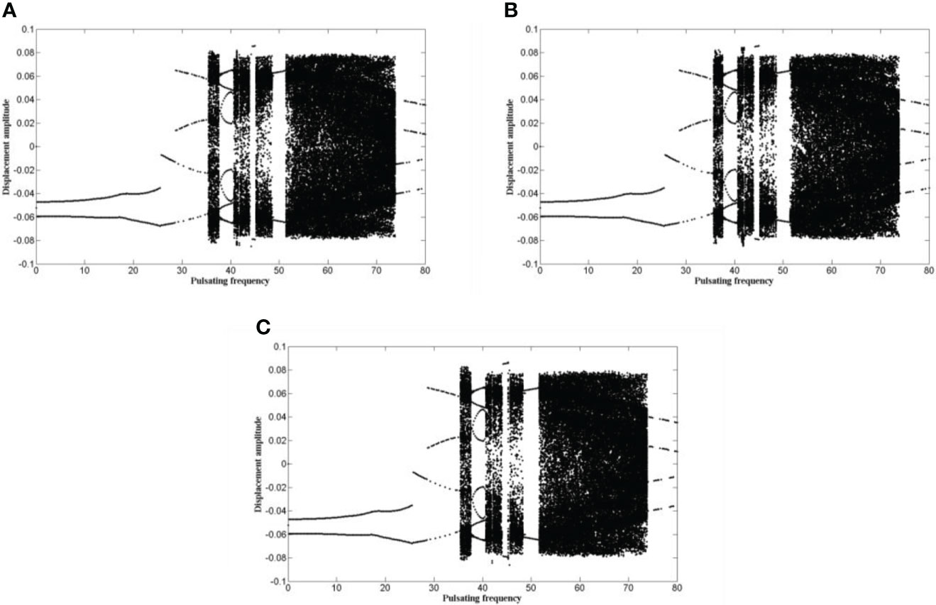
Figure 3 The bifurcation diagrams for the midpoint of the pipe, under different Galerkin truncations N (in which υ=8, u_{0 =} 4.5 and the control parameter is ω_p): (A) N=4; (B) N=6; (C) N=8.

4.2 Solution procedure validation

4.2.1 Simplified modelI: The pipe has no axial motion

In this part, the simplified model is introduced to further verify the solution procedure. First, consider that the pipe has no axial motion, namely, $\upsilon =0,\dot{\upsilon }=0$. Utilizing almost the same system parameters by Ni et al. (2014), i.e.,

β₁ = 0.64, β₂ = 0.36, β₃ = β = 0, u₀ = 4.5, and taking pulsating frequency as the control parameter, the bifurcation diagram result is obtained and shown in Figure 4. Comparing Figure 4A with a figure in the previous work [Figure 2 in the work of Ni et al. (2014)], the results are nearly the same: The main difference lies in the magnitude of the displacement, which may be caused by the different damping values.

FIGURE 4

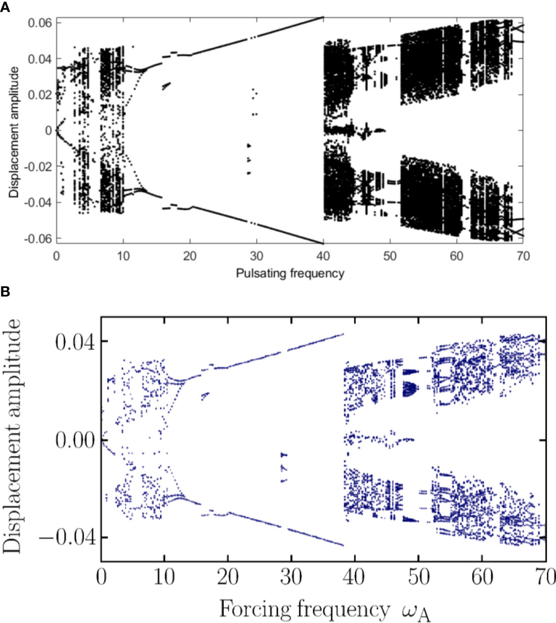
Figure 4 The bifurcation diagrams for the midpoint of the pipe with static supports: (A) the present work; (B) Figure 2 in the work of Ni et al. (2014).

4.2.2 Simplified modelII: Axially moving pipe but no internal fluid

Then, consider that there is no internal fluid, namely, u=0, $\dot{u}$=0, the pipe system is degenerated to the corresponding beam system. Utilize the same system parameters and the initial conditions by Li and Ni (Li et al., 2015), i.e., q_j = 0.001, j = 1 ∼ 4; q_j = 0, j = 5,6…N; ${\dot{q}}_j=0$, j = 1,2…N; β₁ = 0, β₂ = β₃ = 0.5, β = 0.2, κ = 20000 where the Galerkin truncation N = 8. Taking moving speed as the control parameter, the bifurcation diagram result is obtained and shown in Figure 5. Comparing Figure 5A with a figure in the previous work [Figure 8A in the work of Li and Ni (Li et al., 2015)], the results are totally the same.

FIGURE 5

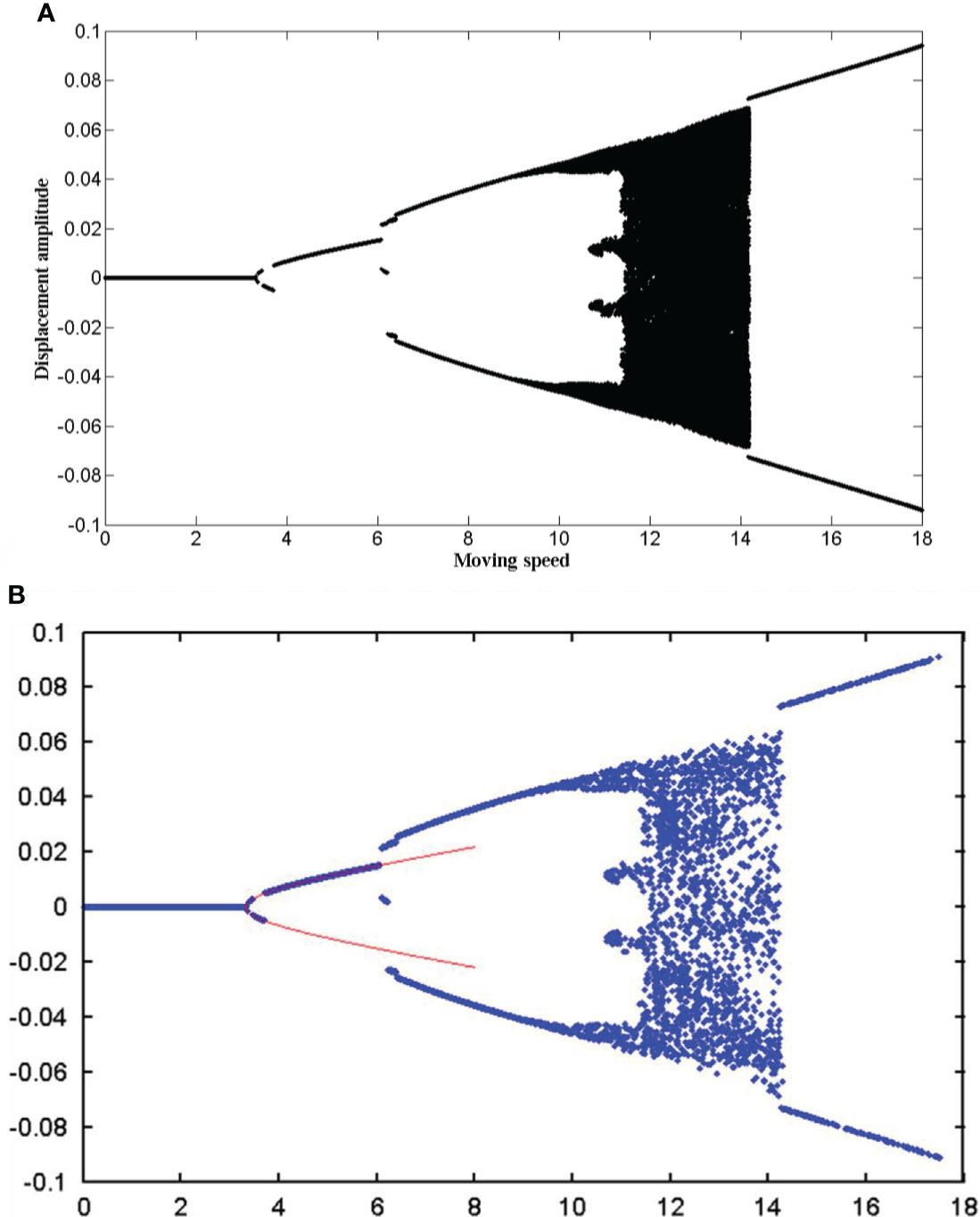
Figure 5 The bifurcation diagrams for the midpoint of the pipe, irrespective of the internal fluid: (A) the present work; (B) Figure 2 in the work of Li and Ni (Li et al., 2015).

5 Results

5.1 Linear dynamic

In this part, the effect of non-linear additional pipe axial force and pulsating internal flow is not considered; the linear dynamic of the system is studied first. For linear dynamic, the matrix form of Equation (8) is degraded into

$\begin{array}{ll}\mathbf{\text{M}}\ddot{\mathbf{q}}+\mathbf{\text{C}}\dot{\mathbf{q}}+\mathbf{Kq=0}& (23)\end{array}$

Then, the solution of Equation (23) can be expressed as:

$\begin{array}{ll}\mathbf{\text{q=}}\overline{\mathbf{q}}\exp (\omega \tau )& (24)\end{array}$

where ω is the non-dimensional frequency. Substituting Equation (24) into Equation (23), for non-trivial solution of the equation, the determinant of the coefficient matrix should be zero, that is,

$\begin{array}{ll}\det \mathbf{(}{\omega }^{\mathbf{2}}\mathbf{\text{M}}+\omega \mathbf{\text{C}}+\text{K})=0& (25)\end{array}$

By solving Equation (25), the eigenvalues of system can be obtained, where the imaginary part of the eigenvalues represents the natural frequencies and the real part is associated with the damping.

Before results are presented, several kinds of critical value need to be introduced (Ni et al., 2017).

υ_Bi, u_Bi: the bifurcation critical value of the ith mode. The imaginary part of eigenvalue (i.e., natural frequency) of the ith mode is reduced to zero completely at this critical speed while the bifurcation of the real parts of eigenvalue occurs.

υ_Di, u_Di: the divergence critical value of the ith mode. Both the imaginary part and the real part (if the bifurcation has been occurred, we say one branch of the real parts) of the ith mode are equal to zero at this critical speed and static buckling of the mode occurs in this case.

υ_Fi, u_Fi: the flutter critical value of the ith mode. The system loses stability via flutter if the moving speed exceeds this critical speed.

First, let the internal fluid velocity be a constant value, i.e., u = 2; the influences of the moving speed on the first three eigenvalues (denoted as ω_i, i = 1, 2, 3) are investigated, and the results are shown in Figure 6. As can be seen in Figure 6, in the first mode, as the moving speed increases, the system is first stable, then loses stability by divergence, and, finally, loses stability by flutter; in the second mode, the system goes through a process like stable-bifurcation-divergence-flutter; in the third mode, the system is always stable. These processes are different from that in the previous work [Figures 7G, H in (Ni et al., 2017)], attributed to the Kelvin–Voigt viscoelastic damping. These show that the Kelvin–Voigt viscoelastic damping has great influence on the second and third modes but has little influence on the first mode.

FIGURE 6

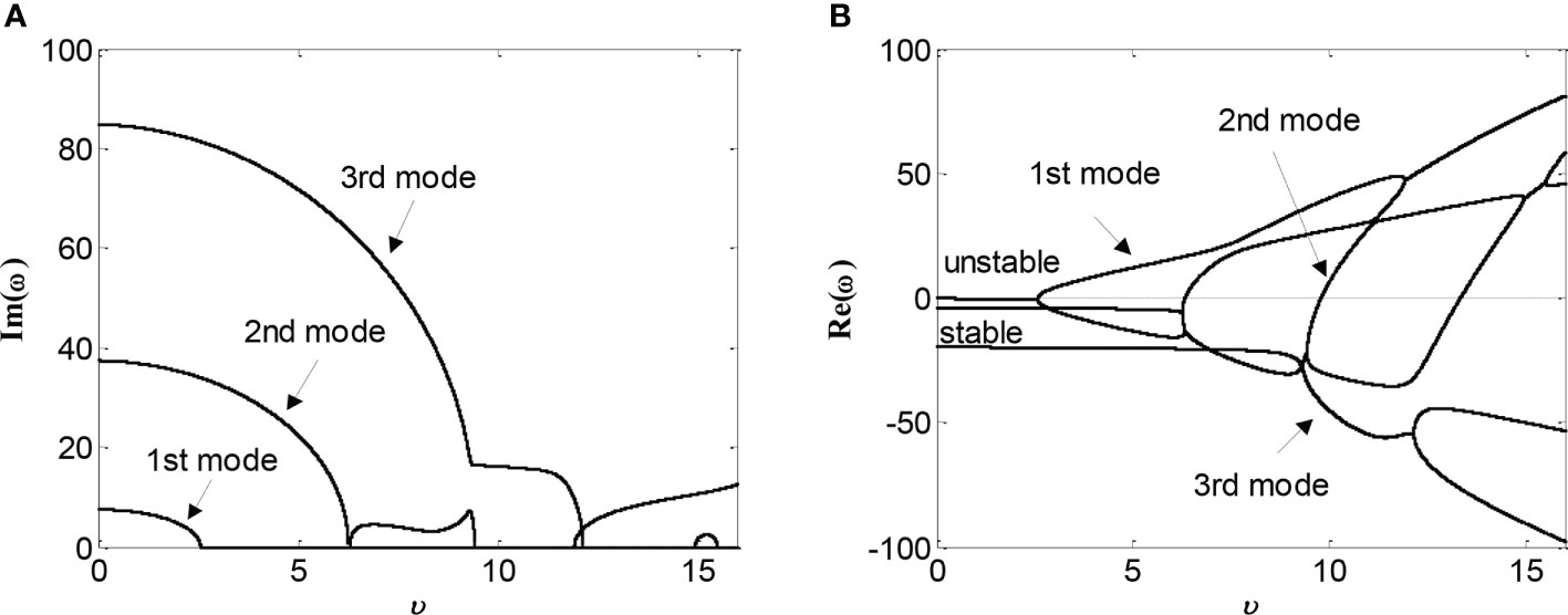
Figure 6 Variations of the non-dimensional frequency ω with the moving speed υ, for the first three modes of pinned-pinned pipe with internal fluid velocity u = 2: (A) the imaginary parts; (B) the real parts.

Several critical speeds of the system are listed as follows: In the first mode, the bifurcation critical speed υ_B1 ≈ 2.559, the divergence critical speed υ_D1 ≈ 2.565, and the flutter critical speed υ_F1 ≈ 11.93; in the second mode, the bifurcation critical speed υ_B2 ≈ 6.256, the divergence critical speed υ_D2 ≈ 9.788, and the flutter critical speed υ_F2 ≈ 14.96.

Then, let the moving speed be a constant value, i.e., υ = 2; the influences of the internal fluid velocity on the first three eigenvalues are investigated, and the results are shown in Figure 7. Comparing Figure 6 with Figure 7, it is easy to find that the influences of the internal fluid velocity are similar to the moving speed. Several critical velocities are listed as follows: In the first mode, the bifurcation critical velocity u_B1 ≈ 2.507, the divergence critical velocity u_D1 ≈ 2.51, and the flutter critical velocity u_F1 ≈ 6.12; in the second mode, the bifurcation critical velocity u_B2 ≈ 8.878, the divergence critical velocity u_D2 ≈ 9.234, and the flutter critical velocity u_F2 ≈ 13.06.

FIGURE 7

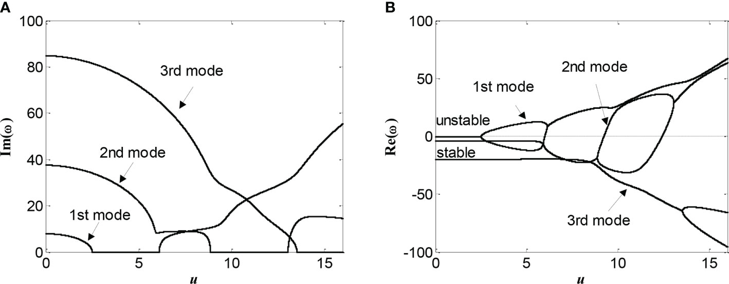
Figure 7 Variations of the non-dimensional frequency ω with the internal fluid velocities u, for the first three modes of pinned-pinned pipe with moving speed υ = 2: (A) the imaginary parts; (B) the real parts.

5.2 Dynamic responses without pulsating internal flow

In this part, the influence of the non-linear additional axial tension on the dynamic response, for the midpoint of the pipe, is investigated. The pulsating component of the internal flow is neglected in this part, i.e., u = u₀. First, consider the internal flow velocity below the divergence critical velocity, i.e., u = 2< u_B1 ≈ 2.507, and take moving speed υ as control parameter, the bifurcation diagram for the midpoint of the pipe is presented in Figure 8. As can be seen in Figure 8, when the moving speed is small, υ ≤ 2.55, the system is stable at the equilibrium position; as the moving speed increases, 2.55< υ< 10.95, the system motion becomes stable around the first bucking mode; as the moving speed goes higher, 10.95 ≤ υ, the system motion becomes symmetric limit cycle motion. Comparing Figure 8 with Figure 7, it is not hard to find that, in most of time, the system motions are quite similar; the difference is that the complicated motions, such as quasi-periodic motion and chaotic motion, do not show up in this part.

FIGURE 8

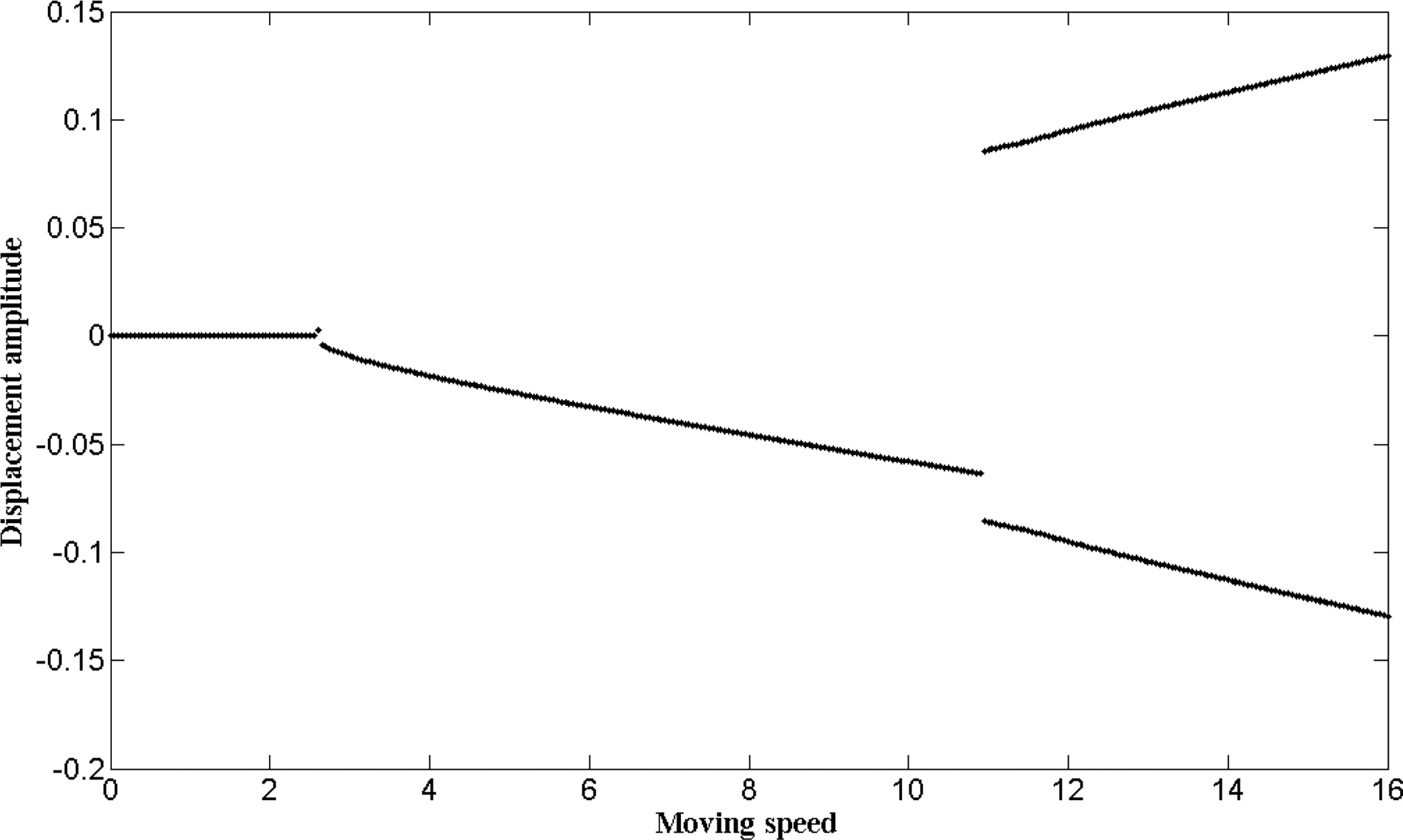
Figure 8 The bifurcation diagram for the midpoint of the pipe (in which u = 2 and the control parameter is the moving speed υ).

Furthermore, time histories and phase portraits of several typical motions are represented in Figure 9. Figures 9A, B represent the equilibrium position; Figures 9C, D represent the bucking mode; Figure 9E, F represent the symmetric limit cycle motion.

FIGURE 9

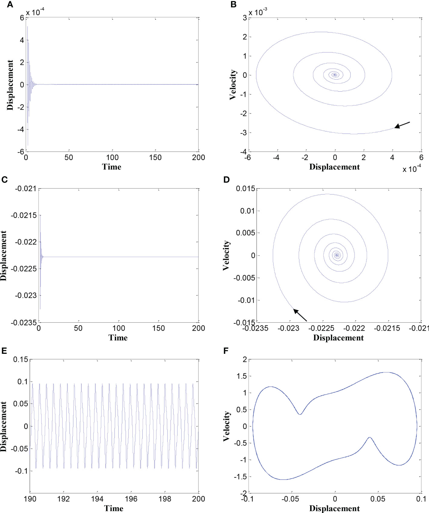
Figure 9 Time histories and phase portraits of several typical motions (in which u = 2). (A, B) υ = 2; (C, D) υ = 4.5; (E, F) υ = 12.

Then, consider the case of the moving speed below the divergence critical velocity, i.e., υ = 2< υ_B1 ≈ 2.559. Take internal flow velocity u as control parameter, the bifurcation diagram for the midpoint of the pipe is presented in Figure 10. As can be seen in Figure 10, the bifurcation diagram is similar to the first case; when the internal flow velocity is small, u ≤ 2.51, the system is stable at the equilibrium position; as the internal flow velocity increases, the system motion becomes stable around the first bucking mode.

FIGURE 10

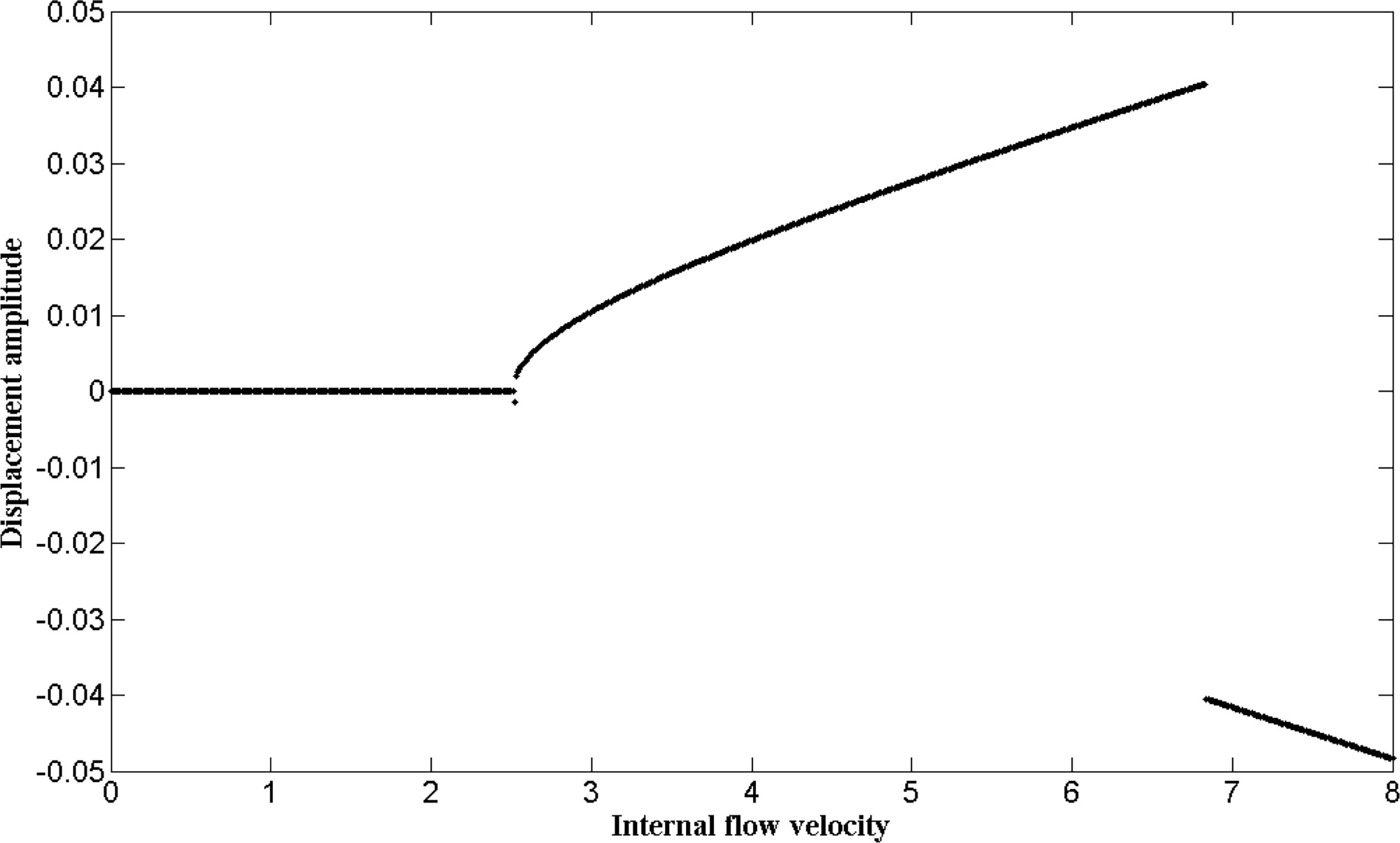
Figure 10 The bifurcation diagram for the midpoint of the pipe (in which υ = 2 and the control parameter is the internal flow velocity u).

5.3 Dynamic responses with pulsating internal flow

5.3.1 Parametric resonance region

According to the analysis in Section 5.1, for linear dynamic, when the internal fluid velocity is taken as u = 2, the divergence critical speed for the first mode is υ_D1 ≈ 2.565; when the moving speed is taken as υ = 2, the divergence critical velocity is u_D1 ≈ 2.51. Therefore, to investigate the influence of the pulsating internal flow, we consider the case with both internal fluid velocity and the moving speed below the divergence critical value, i.e., u = 2 υ = 2. In this case, the first four natural frequencies of the system are listed as follows:

$\begin{array}{ll}{\omega }_1=4.73,{\omega }_2=35.3,{\omega }_3=82.64,{\omega }_4=141.11& (26)\end{array}$

The parameter resonance region of the system with pulsating internal flow is analyzed according to the Floquet theory. Taking the effect of pulsating internal flow into account while neglecting the non-linear axial force, the matrix form of Equation (8) degrades into the form like that in the linear dynamic case, i.e.,

$\begin{array}{ll}\mathbf{\text{M}}\ddot{\mathbf{q}}+\text{C}\dot{\mathbf{q}}+\mathrm{Kq=0}& (27)\end{array}$

Using the state vector

$y={\left\{q,\dot{q}\right\}}^T$, Equation (27) can be transformed into the following form:

$\begin{array}{ll}\dot{\mathbf{y}}\mathbf{\text{=Ay}}& (28)\end{array}$

where

$\begin{array}{ll}\text{A}=\left[\begin{array}{cc}0& \text{I}\\ -M^{-1}K& -M^{-1}C\end{array}\right]& (29)\end{array}$

After considering the effect of pulsating internal flow, the matrix A will be periodic, i.e., A(τ) = A(τ + T), where T represents the period of the pulsating internal flow and T = 2π/ω_p T. Assuming that $\overline{y}$(τ) is one solution of Equation (28), because of the periodic of the matrix A, $\overline{y}$(τ+T) should be another solution of Equation (28), and there exists the following relationship:

$\begin{array}{ll}\overline{\mathbf{y}}(\mathbf{\tau }+\mathbf{T})=\mathbf{\text{Ā}}(\mathbf{\tau })\overline{\mathbf{y}}(\mathbf{\tau })& (30)\end{array}$

where Ā(τ) can be obtained by solving Equation (28) through certain initial conditions as

$\begin{array}{ll}\left[{\overline{y}}_1\left(\tau \right),{\overline{y}}_2\left(\tau \right),\cdots ,{\overline{y}}_{2n}\left(\tau \right)\right]={\left[\begin{array}{llll}1\hfill & 0\hfill & \cdots \hfill & 0\hfill \\ 0\hfill & 1\hfill & \cdots \hfill & 0\hfill \\ ⋮\hfill & ⋮\hfill & \ddots \hfill & ⋮\hfill \\ 0\hfill & 0\hfill & \cdots \hfill & 1\hfill \end{array}\right]}_{2n\times 2n}& (31)\end{array}$

Then, the parameter resonance region of the system can be investigated through the eigenvalue analysis of the matrix Ā(τ) : If the absolute value of all the eigenvalues is less than 1, then the system is stable; otherwise, the parameter resonance instability may occur.

The parameter instability region diagram of the system is shown in Figure 11, in which the abscissa is the pulsating excitation frequency, the ordinate is the pulsating excitation amplitude, and the shadow part in the figure is the area where the system parameter instability occurs. As can be seen in Figure 11, when the pulsating amplitude is small, i.e., μ ≤ 0.1, the system is stable; as the pulsating amplitude increases, when the pulsating frequency is twice the first natural frequency (ω_p ≈ 2ω₁), the first principal parametric resonance occurs; as the pulsating amplitude increases further, when μ ≈ 0.23, the secondary resonance occurs when the pulsating frequency is close to the first natural frequency (ω_p ≈ ω₁); when μ ≈ 0.34, the second principal parametric resonance occurs (ω_p ≈ 2ω₂); when μ ≈ 0.57, the combination resonance occurs (ω_p ≈ ω₁ + ω₂).

FIGURE 11

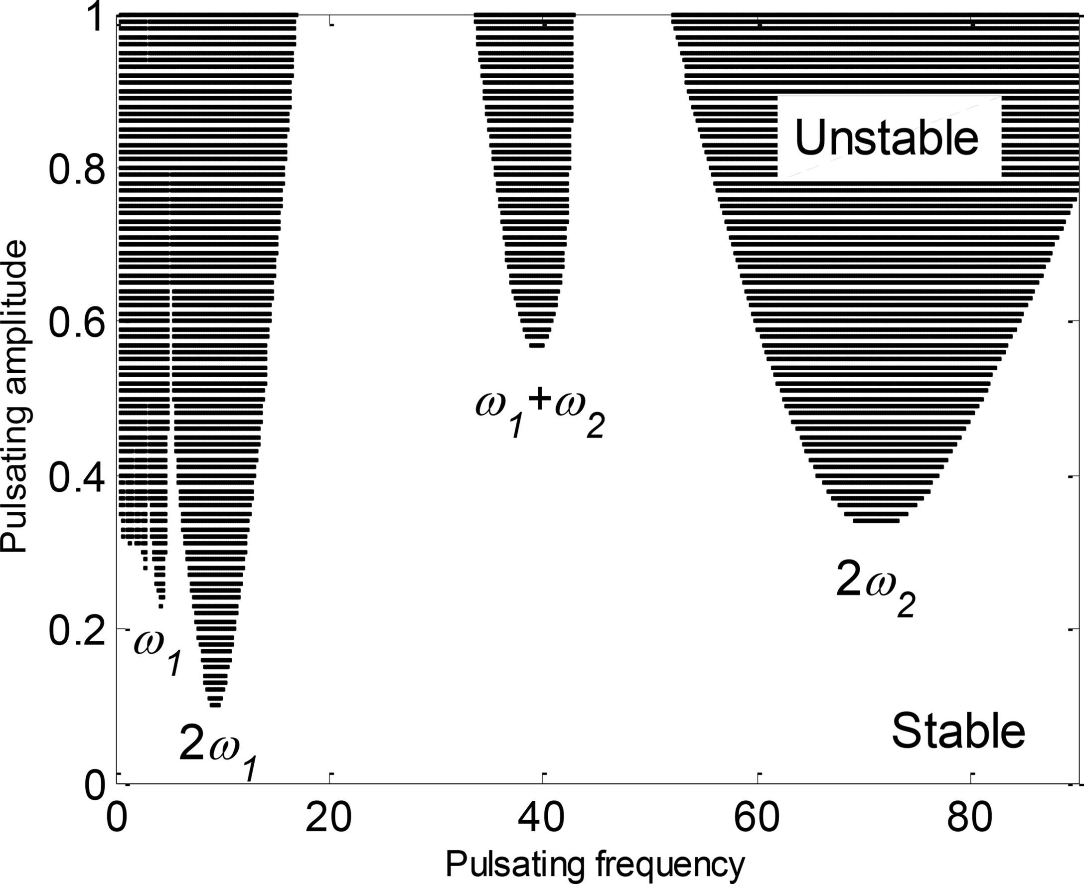
Figure 11 The parameter instability region diagram of the system.

5.3.2 Non-linear dynamic response

In this section, the non-linear dynamic responses of the system are further studied by considering the additional axial tension. In the case where u = 2, υ = 2, the bifurcation diagrams for the midpoint of the pipe with different pulsating amplitudes are shown in Figure 12. When the pulsating amplitude is small, i.e., μ = 0.2, the bifurcation diagram for the midpoint of the pipe is simple, which can be seen in Figure 12A. In most of pulsating frequencies, the system is stable; when ω_p = 7.4, the Hopf bifurcation occurs, and in the range of 7.4 ≤ ω_p ≤ 11.4, the system undergoes period-1 motion, which is caused by the first principal parametric resonance (ω_p ≈ 2ω₁). When μ = 0.4, the bifurcation diagram for the system becomes complex, and the non-linear responses of the system can be denoted as three regions, which can be seen in Figure 12B. Region I indicates the early state of the bifurcation diagram. In region I, the system motions are complicated: When ω_p< 2.75, multiple periodic motion and chaotic motion occur, and these may be caused by low frequency resonance; when 2.75 ≤ ω_{p ≤}5, period-1 motion occurs due to the secondary resonance (ω_p ≈ ω₁). Region II represents that the system is dominated by the first principal parametric resonance, and the system undergoes period-1 motion. Region III represents that the system is dominated by the second principal parametric resonance (ω_p ≈ ω₁), and the system motion is also period-1 motion. When μ = 0.6, the bifurcation diagram for the system is more complicated. When pulsating frequency is small, the system goes from chaotic motion to period-1 motion, but the Hopf bifurcation does not show up between region I and region II. The reason is that the secondary resonance region may be merged with the first principal parametric resonance region. When 37.8 ≤ ω_{p ≤}41, a new region shows up, the Hopf bifurcation occurs due to the combination resonance (ω_p ≈ ω₁ + ω₂), and this region is denoted as region IV. As the pulsating frequency increases, region III and the Hopf bifurcation show up again due to the second principal parametric resonance. The range of region III with μ = 0.6 is much larger than that with μ = 0.4.

FIGURE 12

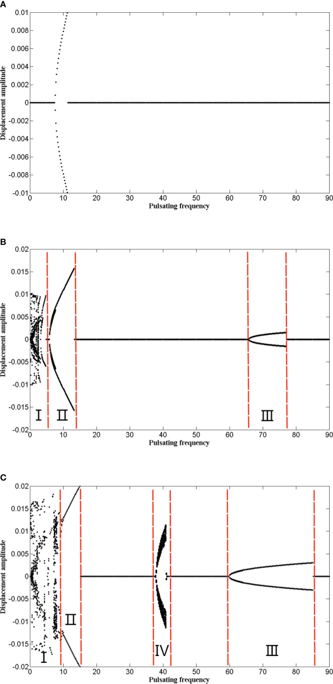
Figure 12 The bifurcation diagrams for the midpoint of the pipe with different pulsating amplitudes (in which u = 2, υ = 2, and the control parameter is the pulsating frequency ω_p). (A) μ = 0.2; (B) μ = 0.4; (C) μ = 0.6.

Because the dynamic behavior of the system is abundant when the pulsating amplitude is large, i.e., μ = 0.6, the displacement and velocity responses of the midpoint of the pipe, when the motion state is stable, are obtained to further analyze the dynamic behavior of the system. Several typical time history and PSD maps of the midpoint of the pipe at different pulsating frequencies are shown in Figure 13. It is noted that the PSD map is unilateral spectrum, where the x-coordinate is the unilateral frequency f = ω_p/2π, where f₁ and f₂ represent the first two order unilateral natural frequencies of the system, respectively. Corresponding phase trajectory maps and Poincaré maps of the system at different pulsating frequencies are shown in Figure 14. As can be seen in Figures 13A, and 14A, when ω_p = 8, the system may undergo chaotic motions: The displacement time curve presents strong randomness; the PSD map shows broadband and noise characteristics; the phase trajectory is a set of curves; the Poincaré map presents a series of dense points with fractal structure. As can be seen in Figures 13B, 14B, when ω_p = 10, the system undergoes period-1 motion: The displacement time curve is simply periodic; the PSD shows clearly narrow-band characteristics and the peaks are near the odd number of natural frequencies corresponding to the first principal resonance (f₁, 3f₁, 5 f₁); the phase trajectory is a single closed curve; the Poincaré map only has two points. As can be seen in Figures 13D, 14D, when ω_p = 70, the system motion characteristics are similar to the case when ω_p = 10, and the main difference is that the former system is affected by the second principal parametric resonance; thus, the peaks of PSD are near the frequencies corresponding to the second principal resonance (f₂, 3f₂, 5 f₂). As can be seen in Figures 13C, 14C, when ω_p = 39, the system undergoes quasi-periodic motion: The composition of the displacement time curve and the PSD map are complicated because of the combination resonance (f₁ +f₂); the phase trajectory is a series of closed curves; the Poincaré map presents a closed curve constituted by a series of dense points.

FIGURE 13

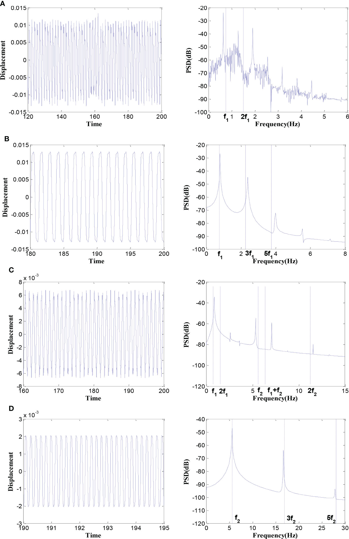
Figure 13 Time history (left) and power spectral density map (right) of the midpoint of the pipe at different pulsating frequencies (when μ = 0.6). (A) ω_p = 8; (B) ω_p = 10; (C) ω_p = 39; (D) ω_p = 70.

FIGURE 14

Figure 14 Phase trajectory map (left) and Poincaré map (right) of the system at different pulsating frequencies (when μ = 0.6). (A) ω_p = 8; (B) ω_p = 10; (C) ω_p = 39; (D) ω_p = 70.

5.3.3 Parametric analysis

In this section, the influence of several key system parameters on the non-linear responses is analyzed, including the axially added mass coefficient, the non-linear axial force parameters, and the system motion parameters. For better studying the influence of the system parameters on the non-linear responses, the values of the internal fluid velocity, the moving speed, and the pulsating amplitude are chosen as u = 2, υ = 2 and μ = 0.6, respectively, and the other system parameters are set on the basis of Equation (21), unless otherwise stated.

5.3.4 The axially added mass coefficient

The influence of the axially added mass coefficient β on the bifurcation diagram for the midpoint of the pipe is shown in Figure 15. As can be seen in Figure 15, the variation of the system motion regions shows great differences. As the axially added mass coefficient β increases, for region I, the displacement amplitude decreases; for region II, the displacement amplitude and the range of the region increase; for region III, the whole region moves a little to the right; for the region IV, the displacement amplitude increases.

FIGURE 15

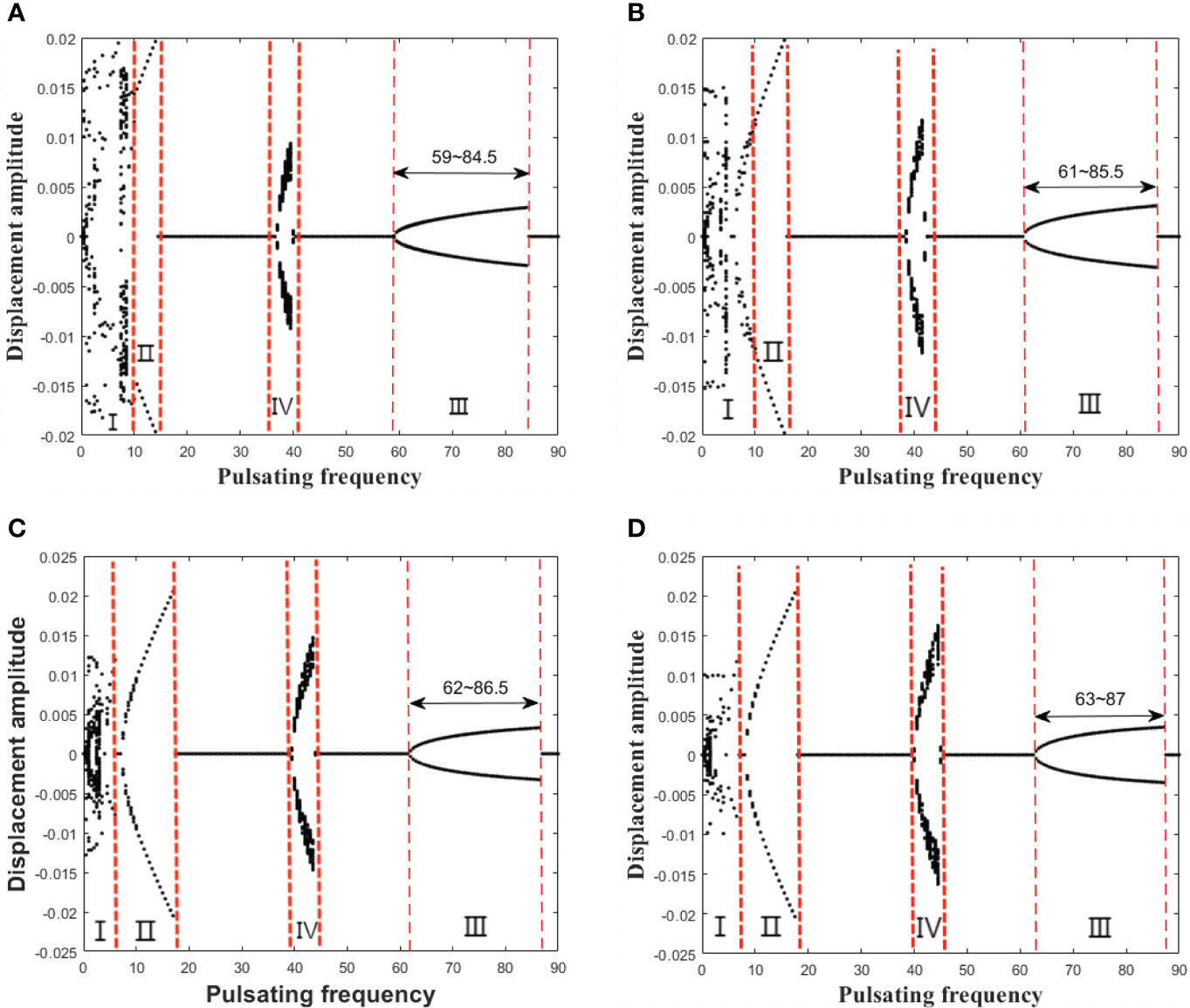
Figure 15 The bifurcation diagram for the midpoint of the pipe with axially added mass coefficient β (in which u = 2, υ = 2, μ = 0.6, and the control parameter is the pulsating frequency ω_p). (A) β = 0.01; (B) β = 0.03; (C) β = 0.05; (D) β = 0.07.

5.3.5 The non-linear axial force parameter

The non-linear axial force parameters include the non-linear axial force coefficient ҡ and the Kelvin–Voigt damping α. The influence of the non-linear axial force coefficient ҡ on the bifurcation diagram for the midpoint of the pipe is shown in Figure 16. As can be seen in Figure 16, with the increase of the coefficient ҡ, the overall shapes of the bifurcation diagrams do not change much, the displacement amplitudes of all the four regions decrease, and the range of region III increases a little.

FIGURE 16

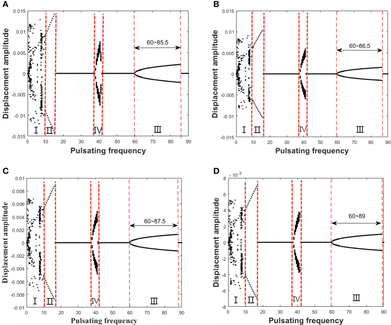
Figure 16 The bifurcation diagrams for the midpoint of the pipe with different non-linear axial force coefficient ҡ (in which u = 2, υ = 2, μ = 0.6, and the control parameter is the pulsating frequency ω_p). (A) ҡ = 10,000; (B) ҡ = 20,000; (C) ҡ = 30,000; (D) ҡ = 50,000.

The influence of the Kelvin–Voigt damping α on the bifurcation diagram for the midpoint of the pipe is shown in Figure 17. As can be seen in Figure 17, with the increase of the Kelvin–Voigt damping α, regions I and II do not change a lot, but regions III, IV, and V show great variations. When α = 0.002, in region III, a new sub-region appears over a narrow frequency range (58.5 ≤ ω_p ≤ 63), which is denoted as region V. In region V, the system undergoes period-2 motion. When α = 0.004, the range of regions III and IV decreases a little. When α = 0.006, regions IV and V both disappear, and the range of region III decreases; when α = 0.008, the range and the displacement amplitude of region III decrease further.

FIGURE 17

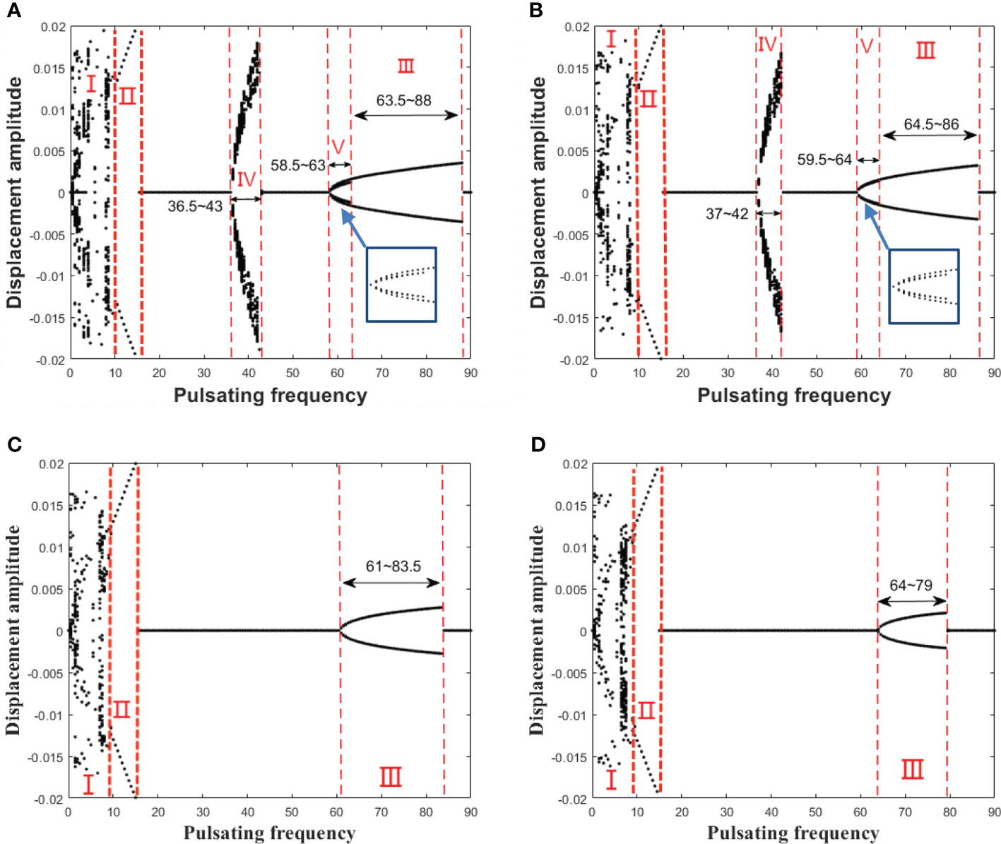
Figure 17 The bifurcation diagrams for the midpoint of the pipe with different Kelvin–Voigt damping α (in which u = 2, υ = 2, μ = 0.6, and the control parameter is the pulsating frequency ω_p). (A) α = 0.002; (B) α = 0.004; (C) α = 0.006; (D) α = 0.008.

5.3.6 System motion parameters

The system motion parameters include the internal fluid velocity u and the moving speed υ. In the cases above, we consider the case of both the internal fluid velocity and the moving speed below the divergence critical value, i.e., u = 2 and υ = 2, respectively. In this subsection, we will first discuss the case that the moving speed is higher than the divergent critical velocity, and the bifurcation diagram is shown in Figure 18. As can be seen in Figure 18, the system motions are very complex: When the pulsation frequency is small (0< ω_p<11), the system motion is periodic, but its equilibrium position is the buckling mode; this kind of motion is so-called the asymmetric periodic motion; then, the system experiences chaotic motion and period-1 motion alternately (11< ω_p<22), where the chaotic motion only occurs a little while; after that, the system undergoes chaotic motion in a long region (22< ω_p<29.5); as the pulsation frequency increases further (ω_p<30), the system returns to asymmetric periodic motion.

FIGURE 18

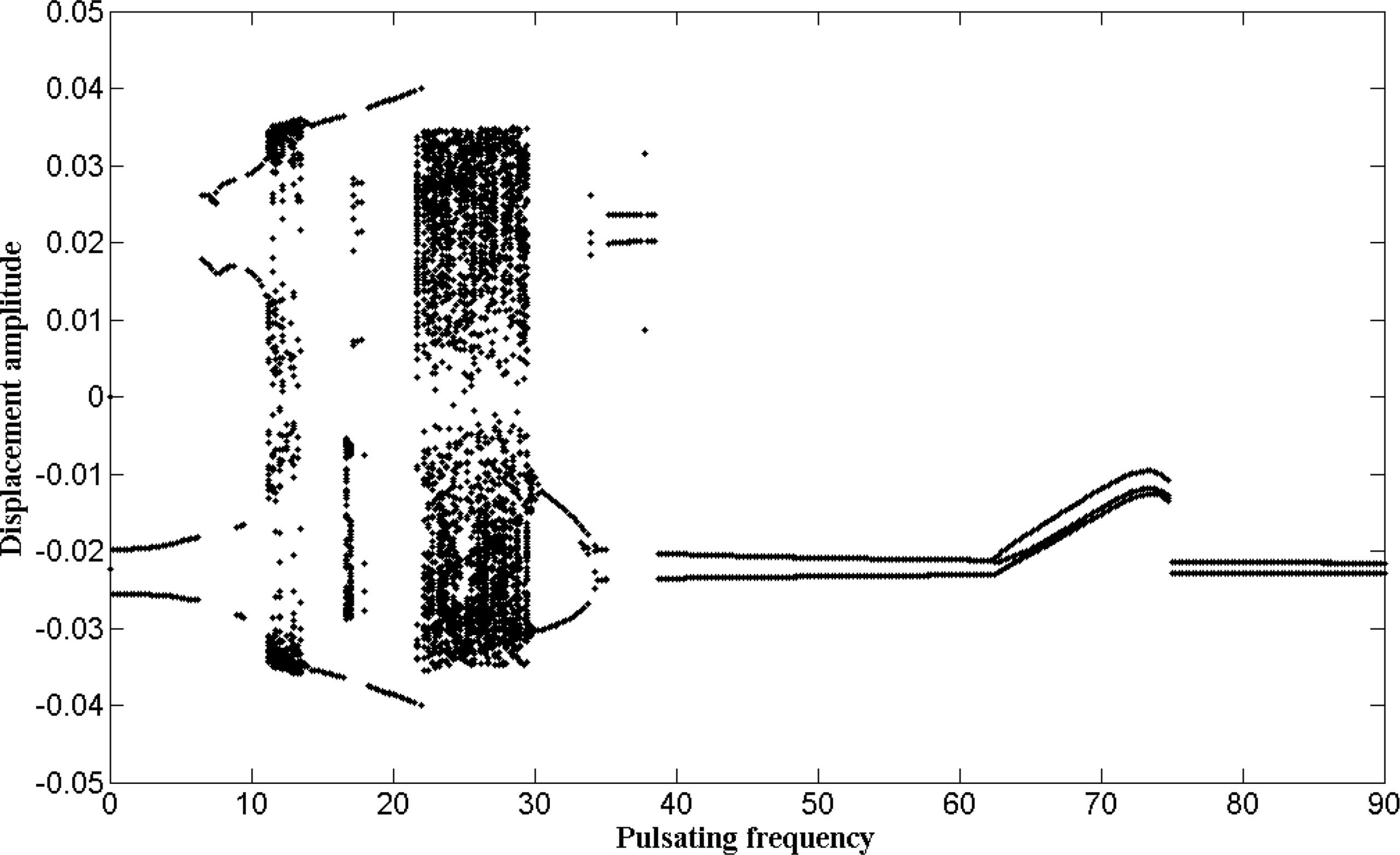
Figure 18 The bifurcation diagram for the midpoint of the pipe when the moving speed is higher than the divergent critical velocity (in which μ = 0.6, u = 2, υ = 4.5, and the control parameter is the pulsating frequency ω_p).

Then, the case that the internal fluid velocity is higher than the divergent critical velocity is also discussed, and the bifurcation diagram is shown in Figure 19. As can be seen in Figure 19, the system motions are more complex: When the pulsation frequency is small (0< ω_p<12), the system undergoes asymmetric periodic motion briefly; then, the system experiences chaotic motion and period-1 motion alternately; this region is similar to the early region in Figure 18; after that, the system undergoes period-1 motion in a long region (12< ω_p<38); then, the system undergoes chaotic motion, multiple periodic motion, and quasi-periodic motion (39< ω_p<60); these two regions are quite similar to the corresponding regions (12< ω_p<60) in Figure 4; as the pulsation frequency increases further (ω_p<65), the system goes through multiple periodic motion and period-1 motion and finally returns to asymmetric periodic motion.

FIGURE 19

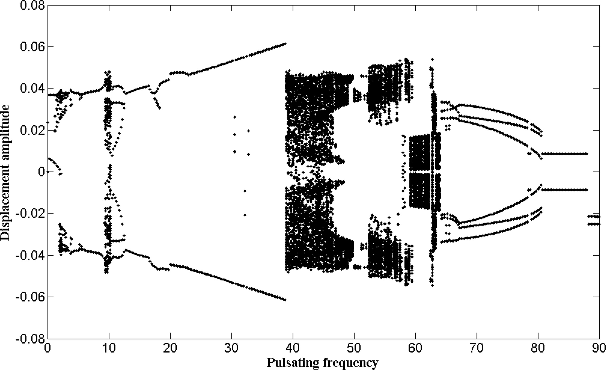
Figure 19 The bifurcation diagram for the midpoint of the pipe when the internal fluid velocity is higher than the divergent critical velocity (in which μ = 0.6, u = 4.5, υ = 2, and the control parameter is the pulsating frequency ω_p).

6 Conclusion

In this paper, both linear and non-linear dynamics of a slender and uniform pipe conveying pulsating fluid, which is axially moving in an incompressible fluid, are comprehensively studied. The vibration equations of the system are established by considering various factors, including a coordinate conversion system, an “axial added mass coefficient” describing the additional inertia forces caused by the external fluid, the Kelvin–Voigt viscoelastic damping, a kind of non-linear additional axial tension, and the pulsating internal fluid. The vibration equations are discretized by the Galerkin procedure and solved by the Runge–Kutta approach, and the validity of the solution procedure is carefully checked. After that, the linear and non-linear responses of the system are studied deeply, especially the non-linear responses of the system under the pulsating internal flow. The results of this paper reveal many new phenomena.

First, the linear response of the system is studied without considering the non-linear additional pipe axial force and the pulsating internal flow. The variations of the first three eigenvalues under varied moving speeds and internal fluid velocities are investigated, respectively. The critical velocities of the system are obtained as well. Moreover, the results show that the Kelvin–Voigt viscoelastic damping has greater influences on the second and third modes than that on the first mode.

Second, the non-linear dynamic response is studied considering the non-linear additional pipe axial force while the pulsating component of the internal flow is neglected. The results show that the bifurcation diagram of the system is simple compared with that in the previous study (Li et al., 2015); the complicated motions, such as quasi-periodic motion and chaotic motion, do not show up.

Third, the non-linear dynamic responses of the system under pulsating internal flow are studied. The parameter instability region diagram of the system is obtained on the basis of the Floquet theory, and the system motions in the corresponding regions are investigated by bifurcation diagram, time history curve, PSD, phase trajectory, and Poincaré map. The results show that, as the pulsating amplitude increases, the system will experience the first and second principal parametric resonances, the secondary resonance, and the combination resonance. Moreover, abundant system motions can be observed, including period-1 motion, quasi-periodic motion, and chaotic motion. Finally, the influence of several key system parameters on the non-linear responses is analyzed.

Data availability statement

The original contributions presented in the study are included in the article/supplementary material. Further inquiries can be directed to the corresponding author.

Ethics statement

This article does not contain any studies with human participants or animals performed by any of the authors. Informed consent was obtained from all individual participants included in the study.

Author contributions

Conceptualization, YL and DZ; methodology, YL; validation, YL; data curation, YL and DZ; writing-original draft preparation, YL; writing-review and editing, DZ. All authors have read and agreed to the published version of the manuscript.

Acknowledgments

The financial support from the Program For Scientific Research Start-Up Funds Of Guangdong Ocean University (R19020) and the Science and Technology Project of Zhanjiang City (2020B01465) to this work is gratefully acknowledged.

Conflict of interest

The authors declare that the research was conducted in the absence of any commercial or financial relationships that could be construed as a potential conflict of interest.

Publisher’s note

All claims expressed in this article are solely those of the authors and do not necessarily represent those of their affiliated organizations, or those of the publisher, the editors and the reviewers. Any product that may be evaluated in this article, or claim that may be made by its manufacturer, is not guaranteed or endorsed by the publisher.

References

Balakrishnan A. V. (1985). A mathematical formulation of a large space structure problem. Proceedings of 24th Conference on Decision and Control, December 1985 (Ft. Lauderdale, FL).

Google Scholar

Du H., Hitchings D., Davies G. A. O. (1992). A finite element structural dynamics model of a beam with an arbitrary moving base–part I: Formulations. Finite Elements Anal. Design 12 (2), 117–131. doi: 10.1016/0168-874X(92)90059-L

CrossRef Full Text | Google Scholar

Gerstmayr J. (2013). Review on the absolute nodal coordinate formulation for large deformation analysis of multibody systems. J. Comput. Nonlinear Dynam. 8 (3), 031016. doi: 10.1115/1.4023487

CrossRef Full Text | Google Scholar

Ginsberg J. H. (1973). The dynamic stability of a pipe conveying a pulsatile flow. Int. J. Eng. Sci. 11 (9), 1013–1024. doi: 10.1016/0020-7225(73)90014-1

CrossRef Full Text | Google Scholar

Gosselin F., Paıïdoussis M. P., Misra A. K. (2007). Stability of a deploying/extruding beam in dense fluid. J. Sound Vib. 299, 123–142. doi: 10.1016/j.jsv.2006.06.050

CrossRef Full Text | Google Scholar

Huo Y. L., Wang Z. L. (2016). Dynamic analysis of a vertically deploying/retracting cantilevered pipe conveying fluid. J. Sound Vib. 360, 224–238. doi: 10.1016/j.jsv.2015.09.014

CrossRef Full Text | Google Scholar

Hyun S. H., Yoo H. H. (1999). Dynamic modelling and stability analysis of axially oscillating cantilever beams. J. Sound Vib. 228 (3), 543–558. doi: 10.1006/jsvi.1999.2427

CrossRef Full Text | Google Scholar

Jayaraman K., Narayanan S. (1996). Chaotic oscillations in pipes conveying pulsating fluid. Nonlinear Dynam. 10 (4), 333–357. doi: 10.1007/BF00045481

CrossRef Full Text | Google Scholar

Jin J. D., Song Z. Y. (2005). Parametric resonances of supported pipes conveying pulsating fluid. J. Fluids Structures 20 (6), 763–783. doi: 10.1016/j.jfluidstructs.2005.04.007

CrossRef Full Text | Google Scholar

Kane T. R., Ryan R. R., Banerjee A. K. (1987). Dynamics of a cantilever beam attached to a moving base. AIAA J. Guidance Control Dynam. 10, 139–151. doi: 10.2514/3.20195

CrossRef Full Text | Google Scholar

Li M. W., Ni Q., Wang L. (2015). Nonlinear dynamics of an underwater slender beam with two axially moving supports. Ocean Eng. 108, 402–415. doi: 10.1016/j.oceaneng.2015.08.015

CrossRef Full Text | Google Scholar

Liu J. Y., Hong J. Z., Cui L. (2007). An exact nonlinear hybrid-coordinate formulation for flexible multibody systems. Acta Mechanica Sin. 23, 699–706. doi: 10.1007/s10409-007-0118-x

CrossRef Full Text | Google Scholar

Liu M., Wang Y., Qin T., Zhao J., Du Y. (2021). Nonlinear dynamics of cross-flow tubes subjected to initial axial load and distributed impacting constraints. Shock Vib. 2021, 1–15. doi: 10.1155/2021/2359090

CrossRef Full Text | Google Scholar

Namachchivaya N. S. (1989). Non-linear dynamics of supported pipe conveying pulsating fluid–i. subharmonic resonance. Int. J. Non-linear Mechanics 24 (3), 185–196. doi: 10.1016/0020-7462(89)90037-1

CrossRef Full Text | Google Scholar

Namachchivaya N. S., Tien W. M. (1989a). Non-linear dynamics of supported pipe conveying pulsating fluid–II. combination resonance. Int. J. Non-linear Mechanics 24 (3), 197–208. doi: 10.1016/0020-7462(89)90038-3

CrossRef Full Text | Google Scholar

Namachchivaya N. S., Tien W. M. (1989b). Bifurcation behavior of nonlinear pipes conveying pulsating flow. J. Fluids Structures 3 (6), 609–629. doi: 10.1016/S0889-9746(89)90157-6

CrossRef Full Text | Google Scholar

Ni Q., Li M. W., Tang M., Wang L. (2014). Free vibration and stability of a cantilever beam attached to an axially moving base immersed in fluid. J. Sound Vib. 333, 2543–2555. doi: 10.1016/j.jsv.2013.11.049

CrossRef Full Text | Google Scholar

Ni Q., Luo Y. Y., Li M. W., Yan H.. (2017). Natural frequency and stability analysis of a pipe conveying fluid with axially moving supports immersed in fluid. J. Sound Vib. 403, 173–189. doi: 10.1016/j.jsv.2017.05.023

CrossRef Full Text | Google Scholar

Ni Q., Zhang Z. L., Wang L., Qian Q., Tang M.. (2014). Nonlinear dynamics and synchronization of two coupled pipes conveying pulsating fluid. Acta Mechanica Solida Sin. 27 (2), 162–171. doi: 10.1016/S0894-9166(14)60026-4

CrossRef Full Text | Google Scholar

Öz H. R., Pakdemirli M., Boyaci H. (2001). Non-linear vibrations and stability of an axially moving beam with time-dependent velocity. Int. J. Non-Linear Mechanics 36 (1), 107–115. doi: 10.1016/S0020-7462(99)00090-6

CrossRef Full Text | Google Scholar

Öz H. R., Boyaci H. (2000). Transverse vibrations of tensioned pipes conveying fluid with time dependent velocity. J. Sound Vib. 236 (2), 259–276. doi: 10.1006/jsvi.2000.2985

CrossRef Full Text | Google Scholar

Païdoussis M. P. (1998). Fluid- structure interactions: Slender structures and axial flow, vol. 1 (London: Elsevier Academic Press).

Google Scholar

Païdoussis M. P. (2003). Fluid–structure interactions: Slender structures and axial flow, vol. 2 (London: Elsevier, Academic Press).

Google Scholar

Païdoussis M. P., Issid N. T. (1974). Dynamic stability of pipes conveying fluid. J. Sound Vib. 33 (3), 267–294. doi: 10.1016/S0022-460X(74)80002-7

CrossRef Full Text | Google Scholar

Païdoussis M. P., Li G. X. (1993). Pipes conveying fluid: A model dynamical problem. J. Fluids Structures 7 (2), 137–204. doi: 10.1006/jfls.1993.1011

CrossRef Full Text | Google Scholar

Panda L. N., Kar R. C. (2007). Nonlinear dynamics of a pipe conveying pulsating fluid with parametric and internal resonances. Nonlinear Dynam. 49 (1), 9–30. doi: 10.1007/s11071-006-9100-6

CrossRef Full Text | Google Scholar

Panda L. N., Kar R. C. (2008). Nonlinear dynamics of a pipe conveying pulsating fluid with combination, principal parametric and internal resonances. J. Sound Vib. 309 (3-5), 375–406. doi: 10.1016/j.jsv.2007.05.023

CrossRef Full Text | Google Scholar

Shabana A. A. (1997). Flexible multibody dynamics: Review of past and recent developments. Multibody System Dynam. 1 (2), 189–222. doi: 10.1023/A:1009773505418

CrossRef Full Text | Google Scholar

Taleb I. A., Misra A. K. (2012). Dynamics of an axially moving pipe submerged in a fluid. AIAA J. Hydronautics 15 (1), 62–66. doi: 10.2514/3.63213

CrossRef Full Text | Google Scholar

Taylor G. I. (1952). Analysis of swimming of long and narrow animals. Proc. R. Soc. A 214 (1117), 158–183. doi: 10.1098/rspa.1952.0159

CrossRef Full Text | Google Scholar

Wang L. (2009). A further study on the non-linear dynamics of simply supported pipes conveying pulsating fluid. Int. J. Non-Linear Mechanics 44 (1), 115–121. doi: 10.1016/j.ijnonlinmec.2008.08.010

CrossRef Full Text | Google Scholar

Wang L. (2010). Erratum to "a further study on the non-linear dynamics of simply supported pipes conveying pulsating fluid"[International journal of non-linear mechanics, 2009, 44: 115-121]. Int. J. Non-Linear Mechanics 45 (3), 331–335. doi: 10.1016/j.ijnonlinmec.2009.11.003

CrossRef Full Text | Google Scholar

Wang Y., Hu Z., Wang L., Qin T., Yang M., Ni Q. (2022). Stability analysis of a hybrid flexible-rigid pipe conveying fluid. Acta Mechanica Sin. 38 (2), 521375. doi: 10.1007/s10409-021-09020-x

CrossRef Full Text | Google Scholar

Wang Y., Luo S., Yang M., Qin T., Zhao J., Yu G. (2022). Analysis of marine risers subjected to shoal deep water in the installation process. Polish maritime Res. 29, 43–54. doi: 10.2478/pomr-2022-0016

CrossRef Full Text | Google Scholar

Wang L., Ni Q. (2008). Vibration and stability of an axially moving beam immersed in fluid. Int. J. Solids Structures 45 (5), 1445–1457. doi: 10.1016/j.ijsolstr.2007.10.015

CrossRef Full Text | Google Scholar

Wang Y., Wang L., Ni Q., Yang M., Liu D., Qin T. (2021). Non-smooth dynamics of articulated pipe conveying fluid subjected to a one-sided rigid stop. Appl. Math. Model. 89, 802–818. doi: 10.1016/j.apm.2020.08.020

CrossRef Full Text | Google Scholar

Yan H., Dai H. L., Ni Q., Wang L., Wang Y. K.. (2018). Nonlinear dynamics of a sliding pipe conveying fluid. J. Fluids Structures 81, 36–57. doi: 10.1016/j.jfluidstructs.2018.04.010

CrossRef Full Text | Google Scholar

Yan H., Dai H. L., Ni Q., Zhou K., Wang L.. (2020). Dynamics and stability analysis of an axially moving beam in axial flow. J. Mechanics Mater. Structures 15 (1), 37–60. doi: 10.2140/jomms.2020.15.37

CrossRef Full Text | Google Scholar

Yan H., Ni Q., Dai H. L., Wang L., Li M. W., Wang Y. K.. (2016). Dynamics and stability of an extending beam attached to an axially moving base immersed in dense fluid. J. Sound Vib. 383, 364–383. doi: 10.1016/j.jsv.2016.07.029

CrossRef Full Text | Google Scholar

Yoo H. H., Kim S. D., Chung J. (2009). Dynamic modeling and stability analysis of an axially oscillating beam undergoing periodic impulsive force. J. Sound Vib. 320, 254–272. doi: 10.1016/j.jsv.2008.07.027

CrossRef Full Text | Google Scholar

Zhou K., Dai H. L., Wang L., Ni Q., Hagedorn P.. (2022). Modeling and nonlinear dynamics of cantilevered pipe with tapered free end concurrently subjected to axial internal and external flows. Mechanical Syst. Signal Process. 169, 108794. doi: 10.1016/j.ymssp.2021.108794

CrossRef Full Text | Google Scholar