- 1Centre for Ocean and Atmospheric Sciences, School of Environmental Sciences, University of East Anglia, Norwich Research Park, Norwich, United Kingdom
- 2Centre for Environment, Fisheries and Aquaculture Science (Cefas), Lowestoft, United Kingdom
- 3Natural Environment Research Council (NERC) National Facility for Scientific Diving, Scottish Association for Marine Science, Oban, United Kingdom
- 4Tritonia Scientific Ltd., Dunstaffnage Marine Laboratories, Oban, United Kingdom
Dive computers have the potential to provide depth resolved temperature data that is often lacking especially in close to shore, but spatiotemporal assessment of the robustness of this citizen science approach has not been done. In this study, we provide this assessment for the Red Sea, one of the most dived areas in the world. A comparison was conducted between 17 years of minimum water temperatures collected from SCUBA dive computers in the northern Red Sea (23–30° N, 32–39.4° E), satellite-derived sea surface temperatures from the Operational Sea Surface Temperature and Sea Ice Analysis (OSTIA) optimal interpolation product, and depth-banded monthly mean in-situ temperature from the TEMPERSEA dataset, which incorporates data originating from several in-situ recording platforms (including Argo floats, ships and gliders). We show that dive computer temperature data clearly resolve seasonal patterns, which are in good agreement in both phase and amplitude with OSTIA and TEMPERSEA. On average, dive computer temperatures had an overall negative bias of (–0.5 ± 1.1) °C compared with OSTIA and (–0.2 ± 1.4) °C compared with TEMPERSEA. As may be expected, increased depth-related biases were found to be associated with stratified periods and shallower mixed layer depths, i.e., stronger vertical temperature gradients. A south-north temperature gradient consistent with values reported in the literature was also identifiable. Bias remains consistent even when subsampling just 1% of the total 9310 dive computer datapoints. We conclude that dive computers offer potential as an alternative source of depth-resolved temperatures to complement existing in situ and satellite SST data sources.
Introduction
Long term observations of ocean temperature are essential for our understanding of natural variations and trends caused by climate change (Needler et al., 1999; Rhein et al., 2013), but there is a shortage of depth-resolved temperature data, especially in coastal areas (Wright et al., 2016). Determining temporal and spatial variation via remote sensing in coastal areas is challenging (Baldock et al., 2014). Satellite products are commonly used to measure sea surface temperature (SST) but are affected in coastal areas by proximity of land (Ricciardulli and Wentz, 2004) or aerosol interference (Bernstein, 1982). In addition, satellite SST records only the skin or sub-skin temperature at the sea surface and measurements have been found to differ from in situ measurements by up to 6 °C (Smit et al., 2013) with root-mean-squared errors (RMSE) amplified nearer the coast (Lee and Park, 2020). Although interpolated analysis products are available, it is important to understand how temperature varies with depth for validation of these products (Kennedy et al., 2007).
Public participation in scientific research (Bonney et al., 2009a), often called citizen science, is a rapidly developing field (Bonney et al., 2016). Environmental citizen science projects have been around for well over a century; the first recorded project being the Christmas Bird Count, which has taken place annually in the US since 1900 (Silvertown, 2009). In conjunction with the developing autonomous monitoring technologies, engaging citizen scientists involved in marine recreational activities to gather sub-surface information can help fill the data gap (Hyder et al., 2015; Brewin et al., 2017b; Simoniello et al., 2019). One approach is for citizen scientists to act as sensor platforms (Haklay, 2018), providing crowdsourced ‘Volunteered Geographic Information’ (VGI) (Schade et al., 2010) data for research purposes, such as data from a mobile phone or biosensing watch. Existing initiatives such as the Smartfin project (Brewin et al., 2017a; Brewin et al., 2021) and Sonic kayaks (Action, 2021) utilise sensor data collected from marine recreational activity. In the diving world, dive computers are as ubiquitous as smartphones. With as many as 10 million SCUBA divers world-wide (Wright et al., 2016), most wearing one or more dive computers, there is clear potential for divers to gather depth-resolved information that is difficult to collect by traditional means by following this crowdsourced approach. With sufficient data, dive computers have been found to have an overall mean temperature bias of (−0.2 ± 1.1) °C (Marlowe et al., 2021), offering huge opportunity to contribute to observational datasets, given the potential numbers of available data points worldwide.
Most modern dive computers record profiles of temperature as a function of depth and time, with some older models recording a single minimum temperature for a dive. The Red Sea is one of the top diving destinations in the world (Shaalan, 2005), with in excess of 30 000 dives per year in some areas (Hasler and Ott, 2008). Citizen scientist divers are active in the Red Sea, contributing to projects including monitoring of marine turtles (Mancini and Elsadek, 2018), grey reef sharks (Hussey et al., 2013) and coral reef biodiversity (Branchini et al., 2015). This study collates minimum water temperatures collected from SCUBA dive computers in the northern Red Sea (longitude: 32–39.4° E, latitude: 23–30° N) between 2000 to 2017. These are compared with satellite-derived foundation sea surface temperatures from OSTIA (E.U. Copernicus Marine Service Information, 2020) and in-situ depth-resolved monthly mean observations from TEMPERSEA, which brings together data from CORA (Cabanes et al., 2013) which incorporates profiles from several sources (e.g. Argo, GOSUD, OceanSITES and World Ocean Database) with data sourced from all KAUST (“King Abdullah University of Science and Technology” n.d.) platforms in the Red Sea (e.g. ships, gliders and Argo floats)(Agulles et al., 2019). We establish the quantitative validity of dive computer temperature for resolving seasonal and interannual temperature variations, exploring agreement with satellite and in situ data under different grouping conditions.
Materials and methods
Study area: Red Sea
The Red Sea is a marginal sea formed by continental rifting (Zolina et al., 2017) and has one of the longest reef systems in the world (Fine et al., 2019), at 4000 km (Kleinhaus et al., 2020). 40% of the Red Sea basin is shallower than 100 m, with a maximum depth of 2800 m (Shaked and Genin, 2011). It is economically important for tourism, shipping, oil and gas (Shaltout, 2019), and is a focus for climate science and coral reef research, because of the unprecedented heat tolerance of its scleractinian, reef building corals (Kleinhaus et al., 2020). One of the hottest ocean basins (Abdulla et al., 2018; Krokos et al., 2019), the Red Sea has a pronounced annual temperature cycle (Al-Subhi and Al-Aqsum, 2008). It has an annual mean surface temperature of (27.9 ± 2.1) °C (1982 - 2016) (Shaltout, 2019), with a summer-winter difference of 6 °C (Berman et al., 2003). Interannual variability is greatest in the winter in the north (Karnauskas and Jones, 2018). An SST gradient of 4 °C exists from north to south (Alraddadi et al., 2021), along with a weaker zonal gradient; eastern monthly mean surface temperatures are 0.3 °C higher in the north than on the western side (Al-Subhi and Taqi, 2014). A shallow thermohaline-driven circulation is seen above 150 m (Tragou and Garrett, 1997), with weak semi-diurnal currents in the northern parts (Sofianos and Johns, 2007).
Dive computer data
Dive computers (DC) have temperature bias related to model, pressure sensor location and housing material, but, with aggregation of sufficiently large numbers, a mean bias of -0.2 °C from CTD measured temperature was found (Marlowe et al., 2021). For the present study, 323 088 anonymous data points from unknown dive computers containing date, minimum temperature, maximum depth, latitude and longitude were provided by divelogs.de (Mohr R). These data have been submitted as ‘public’ logbooks and are freely available. While most modern dive computers store full temperature-depth profiles, these were not stored in divelogs.de and were therefore not available for use. However, all dives had a minimum temperature recorded, and we were interested to see the usefulness of this basic dataset. Using anonymous data from an online dive log provided a real test of the potential of raw dive computer data as a useful source for temperature monitoring, where no additional metadata were available about the device, such as model, material, or pressure sensor location.
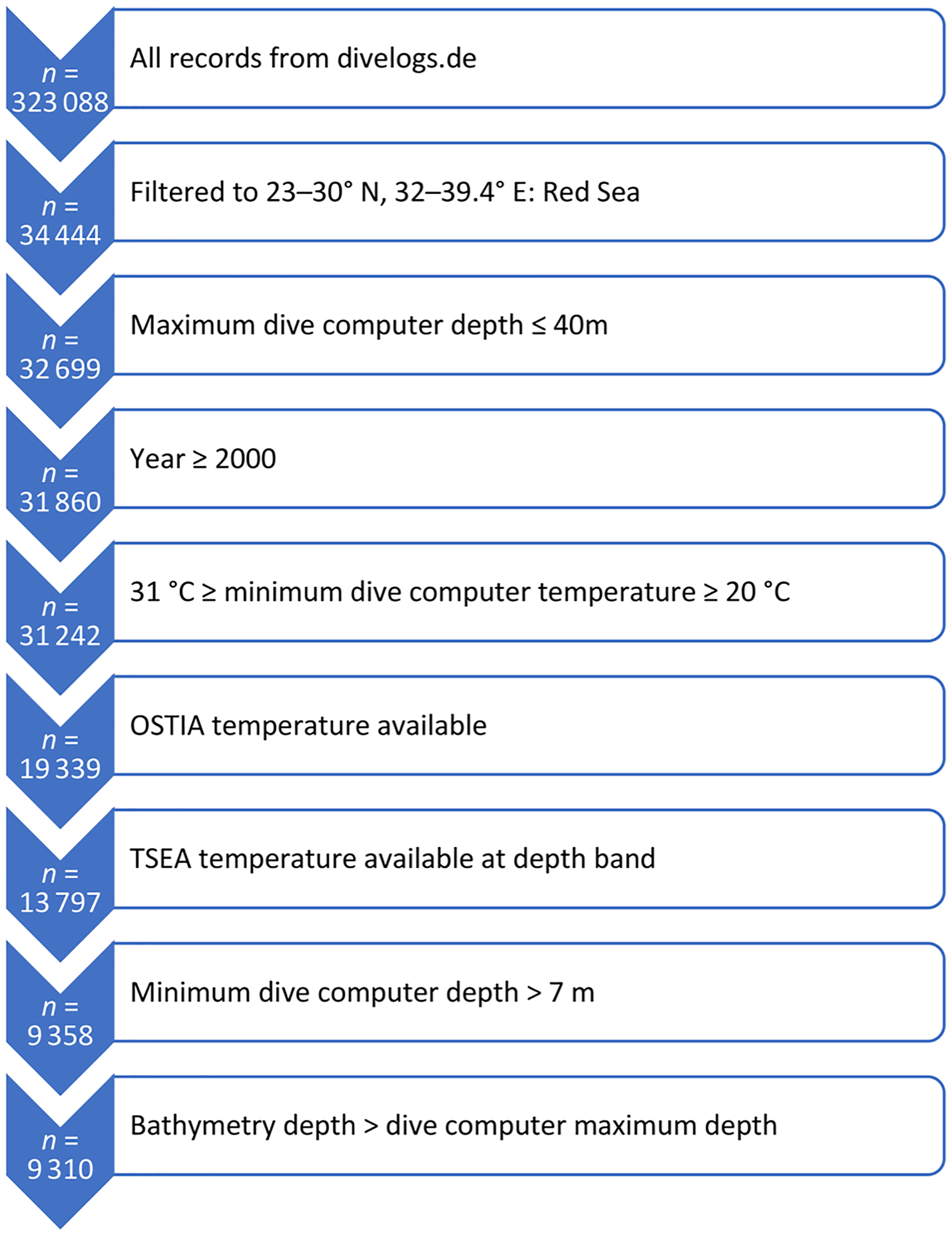
All data were processed in R version 4.2, using the tidyverse suite of packages (tidyverse overview). Basic validity tests were carried out (Figure 1), with the number of dives retained decreasing at each step of the filtering process (Figure 1). The majority of retained dives were in the northern Red Sea. To avoid skewing the comparison (whole region) climatology with temperatures from the warmer southern Red Sea (Fishelson, 1971; Karnauskas and Jones, 2018), the study range was spatially restricted to the northern Red Sea: 23–30° N, 32–39.4° E. Only dives within standard recreational depths (maximum dive depth ≤ 40 m), years with more than 75 dives per year and with a spread of dives across most months were retained (2000 to 2017). Only dives with minimum temperatures between 20 and 31 °C were selected. These temperature constraints were applied as, in the Red Sea, temperatures as low as 20 °C have only been found in water at depths >1500 m (Shaked and Genin, 2011) and >31 °C SST only in the extreme southern Red Sea (Karnauskas and Jones, 2018). Only dives with a collocated OSTIA, and TSEA datapoint at the relevant depth band were retained (further details in section 3.3.3). A 15 arc second-resolution bathymetry (approximately 0.5 km) for the area was downloaded from GEBCO (General Bathymetric Chart of the Oceans) (GEBCO Compilation Group, 2020). Bathymetry depths associated with each dive location were found using the get.depth function in the marmap package in R (Pante et al., 2020). To exclude any incorrectly geolocated dives where the recorded latitude and longitude correlated with land rather than sea, all records for which the corresponding bathymetry depth was shallower than the maximum recorded dive depth were removed. As there were only 48 dives remaining at 7 m or shallower, only dives with maximum depths over 7 m were retained. The study area and retained dives are shown in Figure 2.
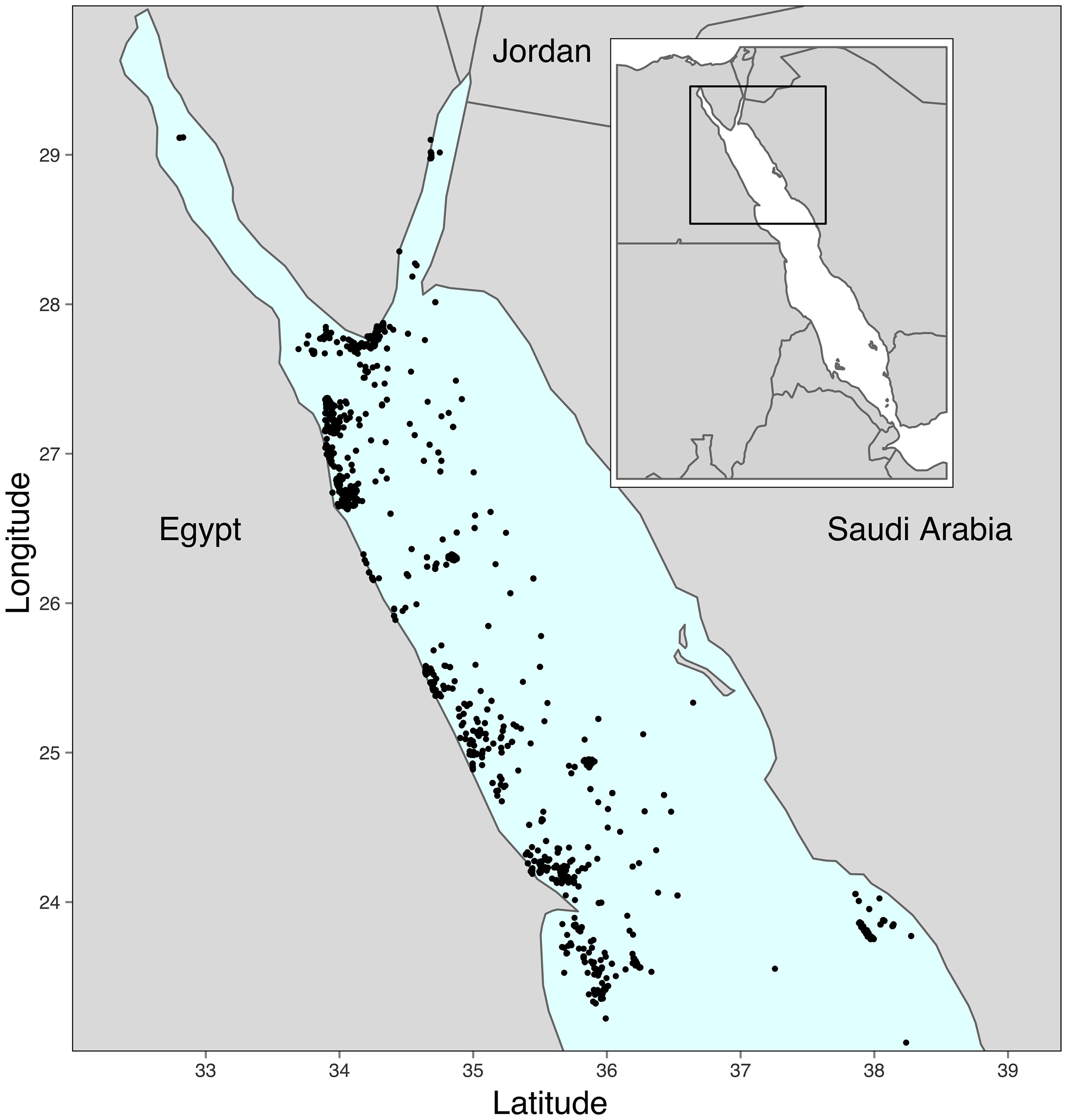
Figure 2 Map of the study region with final selection of dives used in analyses. Inset map shows wider contextual area, with area of interest highlighted with a box.
The Red Sea is an area subject to high solar radiation (Al-Aidaroos et al., 2014) and extremely low precipitation (Abdulla et al., 2018). A cooler surface stratification layer is therefore not expected. Under these conditions, we assumed that the minimum temperature is coincident with the maximum depth. However, during a short dive, a dive computer may have not been at depth sufficiently long to equilibrate to the ambient water temperature (Marlowe et al., 2021). Although an uncommon profile, in a short ‘bounce’ descent to maximum depth followed by an ascent straight back to the surface, the bottom time might be short and artificially high minimum temperatures may be recorded (Wright et al., 2016). No metadata were available about the length of dive, so we have no way to eliminate this potential warm bias in the dive-computer data.
Comparison data
Daily satellite-derived SST data were obtained from the global ocean OSTIA sea surface temperature and sea ice product (E.U. Copernicus Marine Service Information, 2020). This is a level 4 (L4) analysis product (Donlon et al., 2004) with a horizontal resolution of 0.05° x 0.05°, which combines satellite SST data with in-situ data from the HadIOD dataset within an optimal interpolation system (Group for High Resolution Sea Surface Temperature). L4 products are gridded and processed to be gap free, with uncertainty estimates. Foundation SST values were used, which represent the mixed layer temperature (equivalent to 0.2 to 1 m below the surface measured just before sunrise) (Donlon et al., 2012) and therefore removes diurnal variations.
The four nearest OSTIA grid cells by Haversine (or great circle) distance were identified, using the geosphere package in R (Hijmans et al., 2019). A cell is defined as land if greater than 50% of the cell surface is land (Kara et al., 2007). Any returned grid cells with a land mask flag were excluded. An interpolated SST value, θ(sat), for the specified latitude and longitude was calculated from the four grid cells. As bilinear interpolation requires four surrounding data points and many dives were situated along the coastline, to calculate the interpolated value, the inverse distance weighted interpolation function from the Akima package (Gebhardt, 2020) was used.
‘TEMPERSEA’ (TSEA), a 3-D gridded monthly mean 0.25° by 0.25° in situ data product utilizing an optimal interpolation algorithm was used as a reference in situ dataset (Agulles et al., 2019). TSEA has 23 vertical (depth) levels, two within the recreational diving depths of interest in this study (15 and 30 m), plus another one just below, at 50 m. Dive computer data were matched to the TSEA spatial grid at the closest TSEA level below the maximum dive depth, i.e., dive computer data at depths of between 7 and 15 m [θ(DC15)] were compared with 15 m TSEA data [θ(TSEA15)], from 15 m to 30 m [θ(DC30)] were compared with 30 m TSEA data [θ(TSEA30)], and between 30 m and 40 m [θ(DC40)] with TSEA 50 m [θ(TSEA50)]. Values did not exist for all grid cell/depth level combinations. If present, the value (mean monthly temperature at that location/depth) was selected for in situ comparison. Plots of θ(DC) vs. θ(sat), θ(DC) vs. θ(TSEA) and θ(sat) vs. θ(TSEA) were created. Bias was calculated as θ(DC) – θ(sat), θ(DC) – θ(TSEA), or θ(sat) – θ(TSEA).
Monthly and weekly (based on day of year) climatologies of the whole region were produced encompassing the entire temporal and geospatial extent of the study (region). For example, to create a monthly climatology, all daily OSTIA data from all years were aggregated by month and average temperatures produced. These provided baseline seasonal patterns. Mean annual, monthly and weekly values were calculated for each data source for comparison. Anomalies from annual means were calculated for each year and data source (DC, sat, TSEA), to ascertain interannual variation. Amplitudes for each dataset were calculated by year, and each depth band by year, by taking the difference between maximum and minimum mean temperature for each subset. Temporal and spatial resolutions for each data source are summarised in Table 1.
Coastal satellite SST has been found to have poorer agreement with in-situ data (Brewin et al., 2017a). Therefore, we investigated whether dive computer temperature correlated better with satellite data away from the coast. We extracted a 10 m resolution shapefile for the Red Sea coastline from a global coastline shapefile (ne_10m_coastline.shp) (Natural Earth). The shortest distance from dive locations to the coastline were calculated using the sf package in R (Pebesma). As the OSTIA data are on a 0.05° grid, approximating 5.5 km at these latitudes, all dive computer points within 11 km of the coast were categorised as coastal and beyond 11 km as offshore, allowing comparisons to be made between biases based on distance from shore.
Statistical approach
The lm function in R (Carchedi et al.) was used to calculate a simple linear regression between each combination of θ(DC), θ(TSEA) and θ(sat). As uncertainty was present in both variables, York regression was applied to subset data at monthly and weekly resolutions, using the yorkregression function in R (Lichter and Delgado) and using σx and σy for each subset as the error value.
Adjusted R2 ()(was calculated using the Wherry formula 1 as defined by Yin and Fan (Yin and Fan, 2010) (Eq.1) where N is the sample size, p is the number of predictor variables and R is the sample multiple correlation coefficient:
Results
A total of 9310 records with co-located values for θ(DC), θ(TSEA) and θ(sat) were identified (Figure 2). Simple linear regression of θ(sat) vs. θ(DC) (intercept= 1.3 °C, slope = 0.93, =0.78, p =<0.001), θ(TSEA) vs. θ(DC) (intercept= -0.5 °C, slope = 1.01, = 0.65, p =<0.001) and θ(sat) vs. θ(TSEA) (intercept= 7.0 °C, slope = 0.72, = 0.74, p =<0.001) (Figure 3) found θ(sat) and θ(TSEA) respectively explained 78% and 65% of the variation in θ(DC). Mean timeseries bias was (-0.5 ± 1.1) °C for θ(DC) – θ(sat), (–0.2 ± 1.4) °C for θ(DC) – θ(TSEA), and (0.3 ± 1.1) °C for θ(sat) – θ(TSEA).
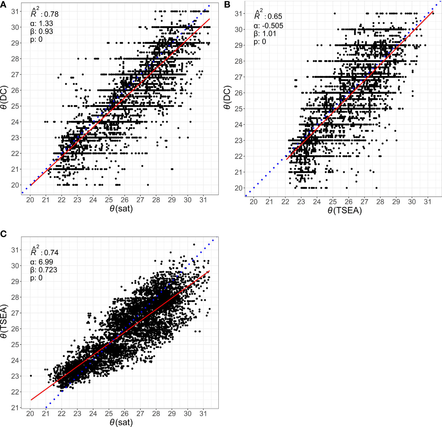
Figure 3 Scatterplot of retained dives (n = 9310). (A) θ(sat) vs. θ(DC), (B) θ(TSEA) vs. θ(DC), (C) θ(sat) vs. θ(TSEA). Linear regression is solid line, dotted line is 1:1 (included as a visual aid).
Dive computer resolution is limited to integers in many models. This is seen in the predominance of dive computer temperatures at integer values in Figure 3. Mean annual SST amplitude was (6.5 ± 1.0) °C for θ(sat). Annual temperature amplitude was comparable for θ(DC15) at (6.8 ± 1.2) °C, and θ(TSEA15) (6.2 ± 0.7) °C.
Monthly resolution
York regression on mean monthly bias showed variation in intercept and slope (Figure 4) but equivalent across all three comparison datasets.
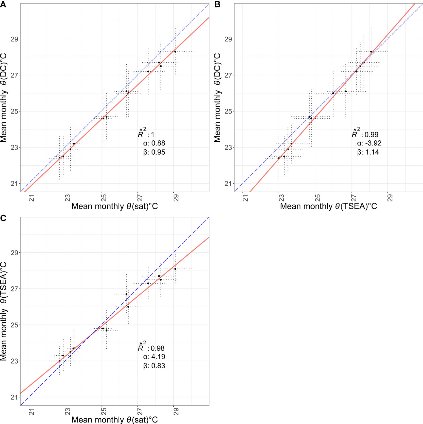
Figure 4 Solid line shows York regression on mean monthly temperature for (A) θ(sat) - θ(DC), (B) θ(TSEA) - θ(DC) and (C) θ(sat) - θ(TSEA), showing intercept α, slope β and R̂2. Dashed line is 1:1. Error bars are standard deviation for a given month/dataset, across all years.
Bias for all three monthly timeseries is shown in Figure 5. The mean maximum depth across all months was consistent at (22.5 ± 1.0) m. The highest biases for θ(DC) – θ(sat) and for θ(sat) – θ(TSEA) were seen in July and August (Figures 5A, C). θ(DC) – θ(sat) bias ranged from (–0.2 ± 1.0) °C in February to (–0.8 ± 1.2) °C in July and August (Figure 5A). θ(DC) – θ(TSEA) bias ranged from (-0.7 ± 0.9) °C in March to (0.0 ± 1.2) °C in May. Absolute mean bias ≤ 0.1 °C was found between May and October (Figure 5B). θ(sat) – θ(TSEA) bias ranged from (-0.4 ± 0.7) °C in March to (1.0 ± 1.3) °C in August, with absolute mean bias ≤ 0.4 °C found between October and April and in June (Figure 5C). Mean monthly temperatures for all data sources show seasonal patterns consistent with those seen in the regional climatology. Seasonal patterns can be seen in overall mean monthly data for each data source, and also individual years (Figure 6)
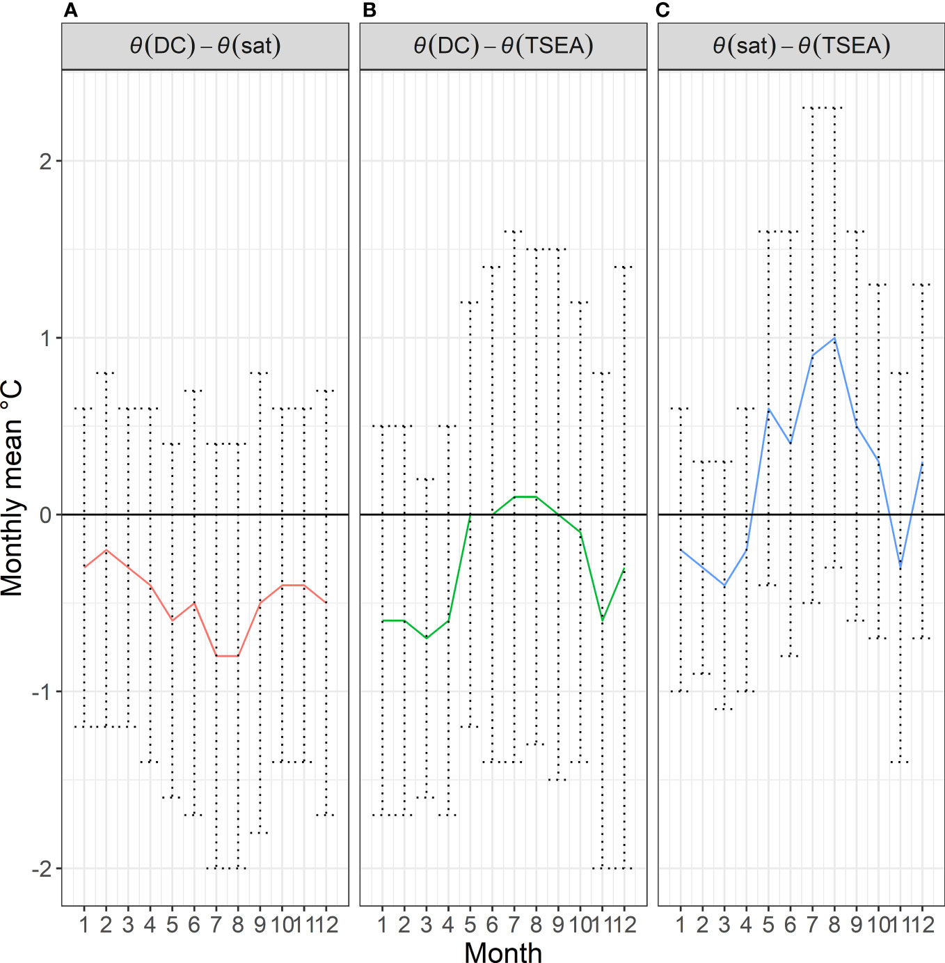
Figure 5 (A) θ(DC) - θ (sat), (B) θ(DC) - θ(TSEA) and (C) θ(sat) - θ(TSEA) bias by month. Error bars show standard deviation for a given month/dataset, across all years.
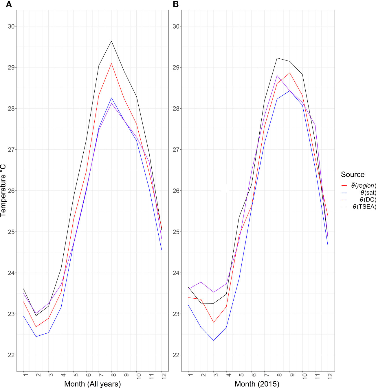
Figure 6 Mean monthly temperatures for θ(DC), θ(sat) and θ(TSEA) with (region) for (A) all years, (B) for an example year (2015).
We also explored bias on a weekly basis, with the same patterns of relative differences observed (See supporting information).
Interannual variation
All-year mean temperatures were θ(DC) = (25.1 ± 2.2) °C, θ(sat) = (25.7 ± 2.3) °C and θ(TSEA) = (25.5 ± 1.8) °C. The annual mean temperature anomalies (annual mean data compared with all-year mean temperature) show consistency (Figure 7). 2003, 2010 and 2016 were warm years across all three timeseries, with 2010 being the warmest (region) year of our study period at (27.1 ± 2.3) °C. This is reflected in θ(DC) and θ(sat), where highest mean annual temperature is also seen for 2010 [θ(DC) = (26 ± 2) °C, θ(sat) = (26.0 ± 2.1) °C]. In contrast, although θ(TSEA) shows 2010 as a warm year at (25.6 ± 1.7) °C, it is only equal third warmest.
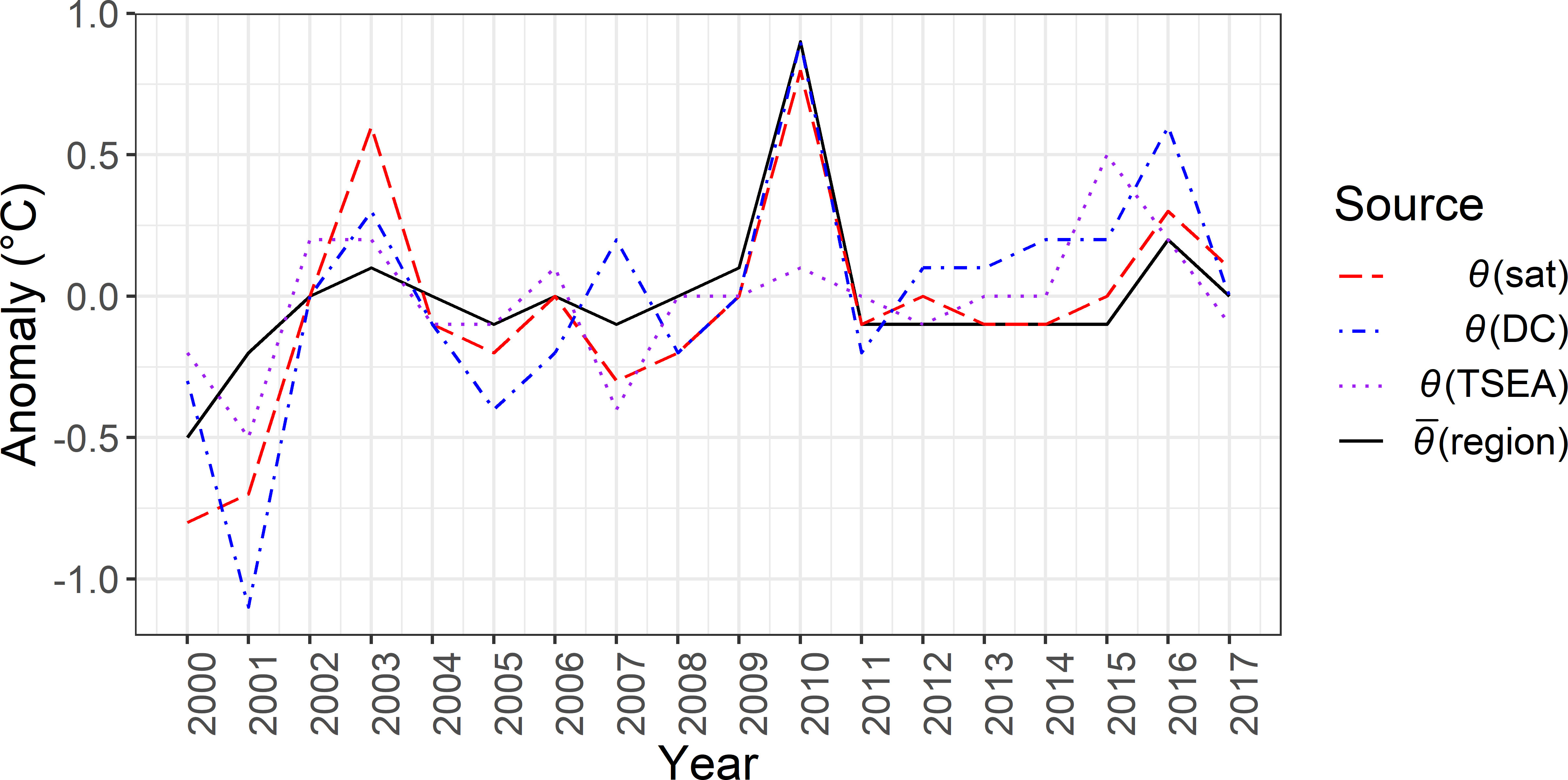
Figure 7 Interannual variation in anomalies from mean θ(DC), θ(sat) and θ(TSEA). Red denotes years that are warmer than average (for the data source) and blue cooler than average.
Months with unusually large anomalies are also comparable across timeseries; for example, the warmest November is 2010 for both θ(sat) (1.5 °C anomaly) and θ(DC) (1.8 °C anomaly), but for θ(TSEA), November 2010 was equal third warmest, with no anomaly from average November temperature.
Latitude bands
In addition to assessing the representativeness of the dataset by comparison with the regional climatology, geospatial and depth effects were investigated. Mean θ(DC), θ(sat) and θ(TSEA) temperature all decreased northwards, except from 28–29° N to 29–30° N (Table 2). Mean θ(DC) – θ(sat) bias ranged from (-0.6 ± 1.0) °C for 23–24° N to (1.1 ± 0.8) °C for 29–30° N, but with bias of –0.6 °C or smaller in the five most southerly bands (Table 2). Mean θ(DC) – θ(TSEA) bias followed a similar pattern, turning increasingly negative northwards, except for the most northerly band (Table 2). Mean θ(sat) – θ(TSEA) bias ranged between (-1.2 ± 0.8) °C for 29–30° N and (0.8 ± 1.3) °C for 24–25° N, with smaller absolute bias in the 25–28° N band.

Table 2 Mean temperature and bias (θ (DC) - θ(sat), θ(DC) - θ(TSEA) and θ(sat) - θ(TSEA) by latitude band.
Distance from coast
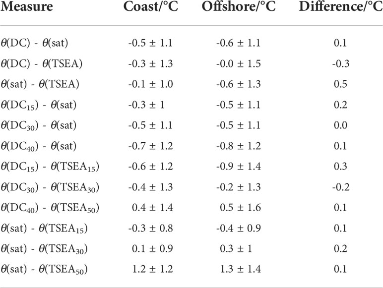
When categorised into coastal (≤ 11 km) or offshore (>11 km) by distance from the coastline, θ(DC) – θ(sat) mean bias was similar for coast and offshore: (-0.6 ± 1.1) vs (-0.5 ± 1.1) °C. θ(DC) – θ(TSEA) bias was smaller offshore by 0.3 °C and θ(sat) – θ(TSEA) was 0.5 °C larger offshore (Table 3). When depth level is included in coastal comparisons, all three data sources showed consistent patterns in direction of temperature bias irrespective of the coastal/offshore category (Table 3). Mean DC depths in the levels (15, 30, 40) m were comparable: (12.6, 21.8, 33.4) m for the coastal dives and (12.7, 23.5, 34.7) m offshore. All biases were 0.1 to 0.3 °C greater offshore, with the exception of θ(DC30) - θ(TSEA30) which had a 0.2 °C smaller offshore bias.
Vertical resolution
The mean DC depth was 12.6 m for θ(DC15), 22.2 m for θ(DC30), and 34.2 m for θ(DC40). When considered in isolation (not including temporal or spatial factors), mean θ(DC) was consistent irrespective of depth: (25.4 ± 2.3) °C for θ(DC15), (25.7 ± 2.3) °C for θ(DC30) and θ(DC40). Although θ(sat) is a foundation temperature and therefore does not have depth level variation, local temperature of the dives will be affected by spatial factors, so it is still a useful comparison, for example, mean comparison satellite temperature was 0.8 °C colder for θ(DC15) dives [θ(sat) = (25.7 ± 2.2) °C] than θ(DC40) [θ(sat) = (26.5 ± 2.2) °C]. Mean θ(TSEA15) °C was (26.1 ± 2.1) °C, reducing to (25.2 ± 1.3) °C for θ(TSEA50). As depth increased, θ(DC) cooled compared with θ(sat) and both θ(DC) and θ(sat) became warmer in comparison with θ(TSEA) (Table 4 and Figure 8).
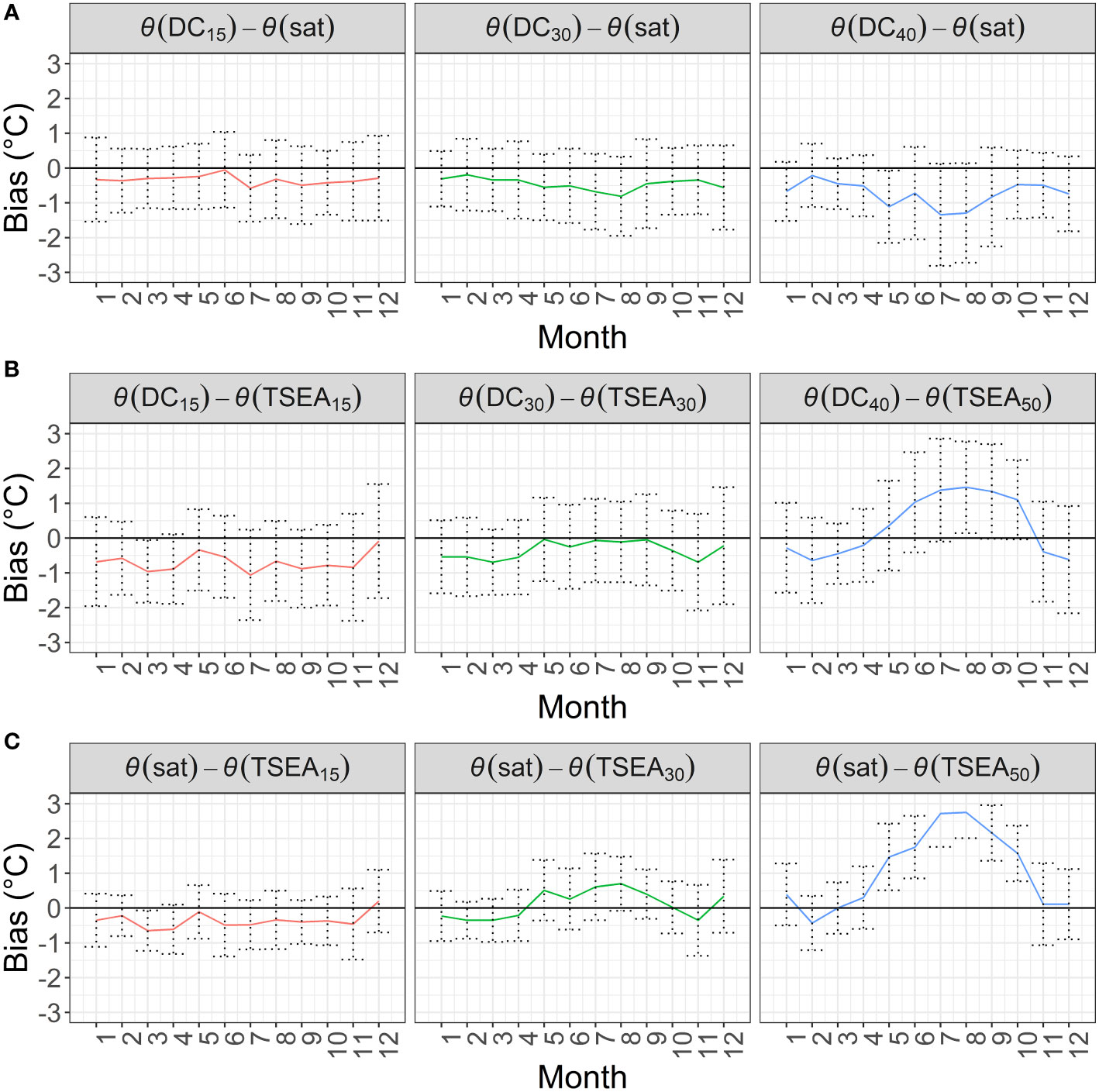
Figure 8 Mean bias by depth and month for (A) θ(DC) - θ(sat), (B) θ(DC) - θ(TSEA), (C) θ(sat) - θ(TSEA).
When taking depth level into account in combination with month, the mean bias shows a clear impact of depth (Table S1 and Figure 8). θ(DC) – θ(sat) bias is negative across all θ(DC) depths. All θ(DC) – θ(TSEA) biases are negative except for θ(DC40) - θ(TSEA50) between May and October (Figure 8). All θ(sat) – θ(TSEA15) and θ(sat) – θ(TSEA30) month biases are negative [θ(sat)< θ(TSEA)] except December [θ(sat) – θ(TSEA15|30)], May and October [θ(sat) – θ(TSEA30)]. All θ(sat) – θ(TSEA50), biases are positive except February.
Group size
To ascertain the number of dive samples required for consistent results, an approach based on a random fraction of samples per year was used. Analysis was run on random samples of different sample fractions (75, 50, 25, 10 and 1%). This generated sample sizes of 6982, 4655, 2328, 931 and 93, respectively. Mean θ(DC) vs. θ(sat) bias remained consistent at (-0.5 ± 1.1) °C at all sample sizes down to 1% (-0.8 ± 1.2) °C. Similarly, θ(DC) vs. θ(TSEA) bias remained consistent with biases of (-0.2 ± 1.4) °C at all sample sizes down to 1% (-0.6 ± 1.5) °C. To check for consistency, from a bootstrap of 50 iterations of 1% (ndives = 93), 36/50 absolute mean biases [θ(DC) - θ(sat)] were ≤0.5 °C, with the remaining 14/50 between 0.5 and 8 °C. 45/50 absolute mean θ(DC) - θ(TSEA) biases were ≤0.5 °C, with 5/50 between 0.6 and 8 °C. 45/50 absolute mean θ(sat) - θ(TSEA) biases were ≤0.5 °C, with 5/50 between 0.5 and 0.7 °C.
Discussion
The Red Sea has a pronounced seasonal temperature cycle (Al-Subhi and Al-Aqsum, 2008). This study utilised a 17-year non-continuous timeseries of in situ and satellite sea temperature data, investigating the potential for temperature data from citizen science logged dives to contribute useful ocean temperatures. We found that temperature data from dive computers can be used to derive interannual patterns in temperature change, and seasonal temperature cycles at monthly and weekly resolutions. These patterns, in agreement with satellite-derived climatology, are consistently seen in timeseries of biases for θ(DC) - θ(sat), θ(DC) - θ(TSEA) and θ(sat) - θ(TSEA). The overall mean θ(DC) - θ(sat) bias of (–0.5 ± 1.1) °C is comparable to the result of Woo and Park (Woo and Park, 2020) who found consistent warm bias in coastal SST of over 0.3 °C in coastal regions when compared with in situ data from buoys, but is in contrast to studies in other areas where a 0.3 °C cool bias in satellite SST was found (Baldock et al., 2014).
Temporal resolution
The overall mean maximum depth of dives was consistent across months at (22.5 ± 1) m. The mixed layer depth (MLD) of the northern Red Sea shows monthly variations (Eladawy et al., 2017). In winter, surface cooling forces convection and a subsequent deepening of the MLD, leading to uniform temperatures around 22 °C (Yao et al., 2014). In summer, surface warming increases SST to over 28 °C, with a coincident reduction of MLD. When surface temperatures are warmest, poorest θ(sat) vs. θ(DC) and greater θ(DC) vs. θ(TSEA) agreement is seen (Figure 6), indicating shallower MLD and increased stratification leading to greater variation in water temperature. This agrees with the MLD climatology (Figure 9); depending on month and latitude, MLD varies from < 20 m to > 80 m, with shallow mean MLDs (< 25 m) in our latitude range mainly observed between April and September (Abdulla et al., 2018). The difference in biases seen by month, in agreement with varying MLD values, demonstrates the importance of depth-resolved data and the potential value dive computers an bring by giving insight into local conditions at depth which is not possible to gather with just sea surface temperature or an interpolated monthly in situ value. Dive durations are unknown, but a likely contributing factor to increased variance in summer months is device heating due to solar radiation prior to the dive.
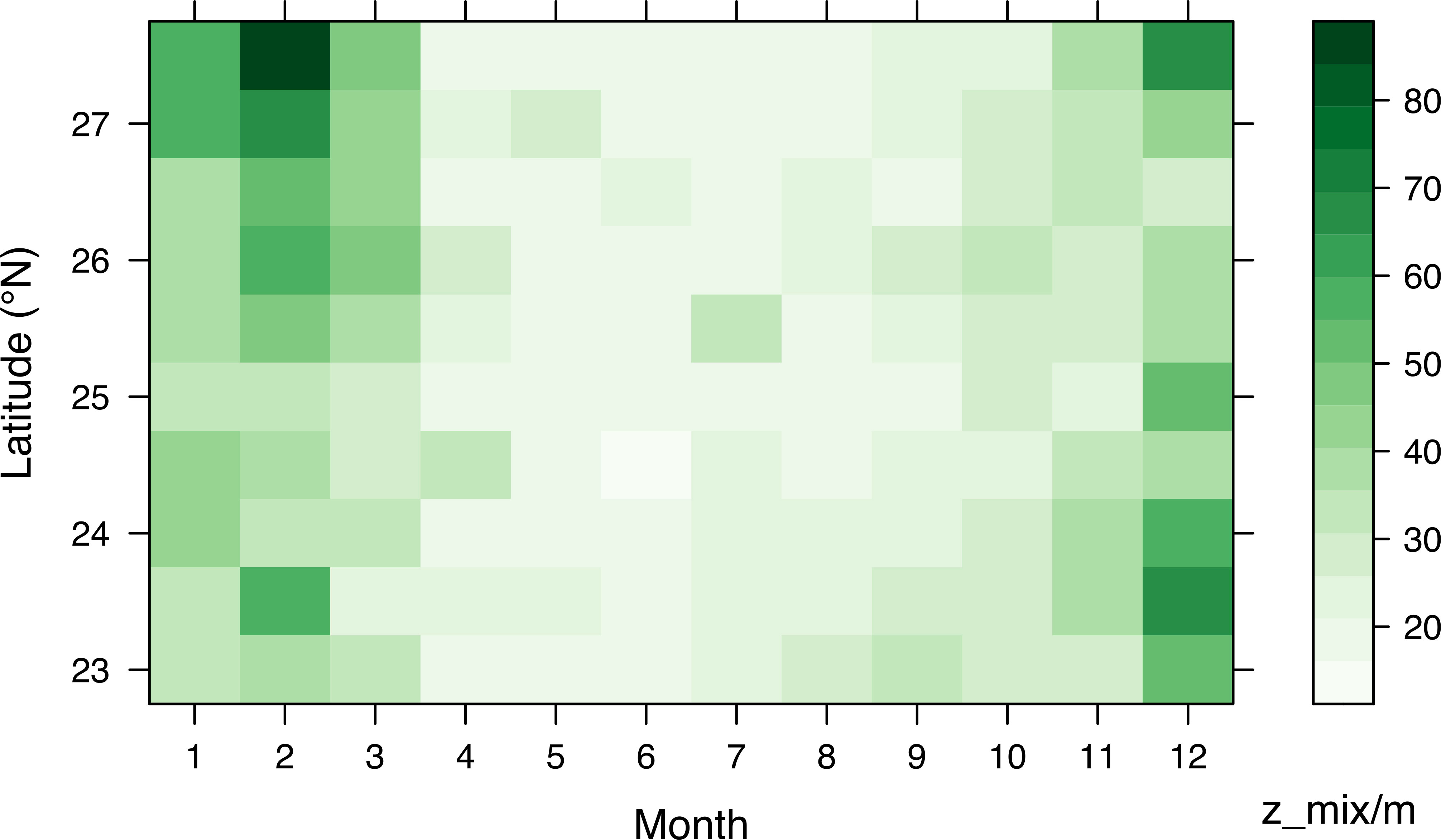
Figure 9 Mixed layer depth by month and latitude (Abdulla et al., 2018).
At a weekly resolution, comparable seasonal patterns are observed (Figure S2). As with monthly comparisons, larger θ(DC) - θ(sat) biases are seen in the summer weeks when surface temperatures are higher and MLD shallower. The reduced consistency in θ(DC) - θ(TSEA) bias seen at weekly resolution is expected as θ(TSEA) has only monthly resolution. θ(sat) interannual variation was largely in agreement with Karnauskas and Jones (2018), with largest SST variations seen in winter. Berman et al. (2003) found a mean surface temperature summer-winter difference of 6 °C. We found amplitudes of 6.4 °C [θ(DC)], 6.5 °C [θ(sat)] and 5 °C [θ(TSEA), amplitude decreasing with increased depth]. This consistency is another demonstrable instance of dive computers producing comparable data to that from more commonly used sources.
Spatial differences
(region) is composed of data across the entire spatial and temporal bounds of the study. Comparing the time series with climatology of the whole region gives insight into seasonal pattern expectations and agreement. The Red Sea is known to display a strong latitudinal temperature gradient from south to north (Chaidez et al., 2017), and a weaker zonal gradient in the north, with eastern monthly mean surface temperatures 0.3 °C higher than the western side (Al-Subhi and Taqi, 2014; Alraddadi et al., 2021). As most dives in our dataset are located near the western coast, this will contribute to the observed bias with the regional climatology (Figure 6). Inspecting latitude bands, we see good spatial agreement, with the latitudinal south – north cooling trend observable in the mean temperatures by latitude band in all datasets, with the consistent exception of the most northerly band. This inconsistency is likely attributable to the small ndives in this band (n = 29).
Satellite SST is purported to have poorer accuracy close to coastlines (Ricciardulli and Wentz, 2004; Smit et al., 2013). As such we would expect to see greater deviation from θ(DC) in data categorised as coastal, but instead see a marginally greater negative bias (-0.1 °C) in the offshore data. However, a L4 analysis product was used as comparison SST, to provide a gap-free dataset. L4 products incorporate data from drifting buoys (E.U. Copernicus Marine Service Information, 2020), to compensate for satellite error, minimising coastal inaccuracies.
Group size
Reducing ndives by random sampling to 1% of the initial 9 310 dives (i.e., 93 dives) did not affect mean bias, standard deviation or values. However, when increasing the granularity by encompassing multiple categories (such as to week by depth level), the number of points reduce to low numbers and the relative importance of the different explanatory variables are less clear. Despite noisy data, significant information about trends is seen, therefore in areas where there are few in situ data alternatives available, small datasets may still offer trend information if care is taken.
Representativeness of data
Representativeness of data is not as simple as merely sample size; individual device factors need to be considered. Drift can occur in forecasting systems as well as citizen science datasets, but sensors utilised for monitoring are usually regularly recalibrated (Bell et al., 2013). Dive computers are not calibrated (after purchase) and use piezoelectric sensors, which are known to drift over time (Otmani et al., 2011). If large volumes of data are collected in a small area from an individual device which has drifted, or has a large systematic bias, overall bias may be seen in the data. In the dataset there are examples of a pattern of morning and afternoon dives, consistent with that of a diving holiday (for example, 10 dives over 5 days), all with a θ(DC) - θ(sat) bias of (-5.1 ± 0.2) °C. In the above example (10 dives in September 2001) a corresponding monthly bias is seen; September 2001 was the coldest September instance for θ(DC) (mean: 24.4 °C), in constrast to both θ(TSEA) and θ(sat) where it was not in the coolest 6 years, and had a mean temperature of 27.7 °C. If a diver is extremely active in logging dives in a particular area, care needs to be taken if there are only a small number of dives logged from other devices. By carrying out regular simple calibration in an ice bucket (Wright et al., 2016), an indication of device bias, and any change over time, could be collected.
Relevance for data usage: Local monitoring
Between 1982 and 2006 the Red Sea experienced warming SST at 5.5 times the global change (Belkin, 2009), but temperature measurement is not straightforward. While Argo floats are commonly used to gather in situ temperature/depth profiles, there are few cycles recorded in the Red Sea, with only 1615 cycles recorded between 2001 and 2021 (Argo 2021), presumably as the single narrow entry point at the Strait of Bab al Mandeb limits their ingress. Mean differences of 0.5 °C have been found between satellite-derived SST products in the Red Sea (Karnauskas and Jones, 2018). Regional variation in coral mortality is affected by local differences in physical parameters (Moore et al., 2012) and Davis et al. (2011) found daily variations ranging from 0.5 °C to >5 °C on shallow Red Sea reefs, depending on the level of protection from waves. As such, micro level data are essential to monitor ambient temperature variation, and its influence on corals and other ecosystem processes (Baldock et al., 2014). With consistent biases being seen between all three datasets at different depths, our findings agree with Colin and Shaun Johnston (2020), identifying depth-resolved temperature differences which are not captured by satellite data. Dive computers therefore are interesting for their potential to provide depth resolved data as they are not limited to nominal depths like sea-surface (satellite) or a fixed depth (in situ sensor). They can offer a valuable additional layer of information at a micro level, to complement data from other sources. Utilising the potential volumes of data that could be available in the highly dived areas of the Red Sea, long term time series could be collated to support monitoring of important corals and their surrounding ecosystems. Further analyses could expand this work, as no comparable case studies of citizen science data exist in other locations.
Practical considerations for dive computer accuracy
Most dive computer models do not have GPS functionality, which introduces potential error in any user recorded coordinates. If a position is recorded to the nearest 0.01° longitude/latitude, the accuracy will be approximately 1 km. The satellite SST grid used here is 0.05°, equivalent to 5.5 km. In addition, the coordinates of the most frequently dived sites are well documented online. Many divers will note the reef or wreck name at the time of dive, looking up coordinates later when back on dry land. In these instances, the potential risk for dive to be recorded at a location greater than 5 km from the actual location is considered small. In less well documented areas, GPS coordinates should be carefully recorded at the start or end of the dive using a GPS tracker or mobile.
Dive computers record time and date, but some require these to be changed manually. If divers travel into a different time zone, and divers do not do this, data are potentially recorded at the wrong time of day. For the purposes of this study, this should not cause an issue because the comparison foundation temperature reflects pre-dawn values. However, a citizen science project would need to consider this where daily variation in temperature is relevant, such as a reef ecosystem. With sufficient data and accurate metadata (such as time zone) from dive computers, in areas with sufficiently large diurnal variation, it could also be possible to gather insight into this variation. By collecting longer term time series of dive computer data, the demonstrated ability to identify anomalously hot or cold periods will become another a valuable source of historical data available for comparison with other biological datasets.
The MS5803-14BA pressure sensor (TE Connectivity, 2017), which is commonly used in dive computers, has sufficient resolution (<0.01) °C to offer improved temperature recording, especially in those models which currently only record temperature in integer intervals. Dive computer models have time constants (time to adjust to 63% total temperature change) ranging between 17 and 300 seconds (Marlowe et al., 2021), which affects the time taken to equilibrate to ambient temperature. In areas of high air temperature, this risks artificially high temperatures being recorded because of surface heating of the device. Knowing the duration of each dive would allow either removal of dives of less than 5 minutes (which is insufficient time to equilibrate to ambient water temperature for some models with slower response time) or based on a known time constant for the model.
Subject to data storage capacity, improving the recorded resolution and recording parameters such as the model and dive duration would ensure that bounce dives or known inaccurate models could be excluded, as features such housing material and pressure sensor location are known to be significant for bias (Marlowe et al., 2021). These would allow better quality control of a dataset and maximise future potential for using dive computers for temperature monitoring. Computers are not calibrated instruments and so sensor temperatures may also drift over time, further research would be required in this area.
Uncertainties and requirements for data
Both comparison datasets used in the study have been interpolated, spatially, using weighted algorithms and/or using background data for gap filling. Uncertainty estimates for individual comparison data points in this study are between 0.16 and 1.07 °C for θ(sat) and between 0.04 and 1.0 °C for θ(TSEA), with the TEMPERSEA dataset having a formal error of 0.31 °C at the surface (Agulles et al., 2019). It is not possible to ascertain the proportion of systematic error in θ(DC) point data from the current dataset and therefore, ad hoc point data is of little use for temperature measurement in isolation. Devices with large bias should still correctly identify seasonal variation, albeit offset. Additionally, the overall absolute mean biases seen of 0.5 °C for θ(DC) - θ(sat) and 0.2 °C for θ(DC) - θ(TSEA) are within the specified uncertainty ranges of the comparison datasets, the proportion derived from each component indeterminable.
The requirements for accuracy, spatial and temporal resolution, and acceptable degree of uncertainty for ocean temperature data varies depending on the intended use (National Research Council, 2000). For example, requirements for monitoring of deep ocean sea temperature are stringent at 0.002 °C (Pawlowicz, 2013), but the World Meteorological Organization (World Meteorological Organization, 2020) only requires SST measurements to 0.1 °C. The three themes of the Global Ocean Observing System (GOOS) have requirements more within reach; climate change detection (0.1 °C on 500 km grid at monthly resolution), operational services (e.g., numerical weather prediction: 0.2 – 0.5 °C accuracy at 100 km grid and 3-day resolution) and ecosystem health (0.2 °C daily) (Needler et al., 1999; Kennedy, 2014; Moltmann et al., 2019). The observed biases indicate dive computers can offer data within the required range for numerical weather prediction and ecosystem health analyses. Observations from buoys stratified to weekly, monthly and seasonal resolutions have been used to identify seasonal patterns, interannual variability and climate signals related to ENSO (McPhaden et al., 2010). Buoys have SST resolution and accuracy of (0.1 ± 1.0) °C (National Data Buoy Centre) and while overall bias in data collected from unknown models is greater than that, the ability to identify seasonal patterns at different resolutions has clearly been demonstrated, and many dive computer models are known to have comparable resolution and accuracy (Marlowe et al., 2021). Thus, a dataset restricted to dive computers with higher accuracy could be used in comparable ways to buoys.
Conclusions
Our results clearly demonstrate that, in the Red Sea, dive computers can resolve interannual variations and seasonal patterns of data comparable with OSTIA and in-situ data. This can provide a layer of insight at varying depths on a local level, over and above that available from other sources. As depth resolved data is key to monitoring of ecosystem processes, we suggest that a database of temperature data derived from SCUBA diver citizen scientists can deliver viable data to complement existing datasets. The consistency between the bias found for subsamples of the total data demonstrate that the numbers of dives do not need to be in the thousands to be produce useful results, with only around 100 datapoints needed for consistency. Data will be most useful in commonly dived areas, giving greater spatial continuity, but in areas with fewer dives and limited or no other monitoring, patterns of data should still be visible from smaller datasets.
Retrospectively analysing data collected without a research question limits the possible analyses (Hochachka et al., 2012), and these limits were seen with the lack of useful metadata such as model of dive computer or dive duration, which could improve overall analyses. However, despite this lack of information our uncontrolled real-world example gave outputs with absolute bias of 0.5 °C and less, identification of months and years with large anomalies and consistent, comparable seasonal patterns at different scales.
Data availability statement
The datasets presented in this study can be found at https://doi.org/10.5285/e5e5c4c7-af59-25df-e053-17d1a68b7f87.
Author contributions
CM carried out the experiments and analyzed the data. CM wrote the manuscript with contributions from all authors. All authors set the conceptual framework of this study. All authors approved the submitted version.
Funding
CM’s PhD project is part of the Next Generation Unmanned Systems Science (NEXUSS) Centre for Doctoral Training which is funded by the Natural Environment Research Council (NERC) and the Engineering and Physical Science Research Council (EPSRC) [grant number: NE/N012070/1]. The PhD project is supported by Cefas Seedcorn [DP901D]. We would also like to thank NERC for additional funding via grant NE/P013899/1 (An Alternative Framework to Assess Marine Ecosystem Functioning in Shelf Seas, AlterEco, https://altereco.ac.uk/).
Acknowledgments
The authors would like to acknowledge divelogs.de for anonymised dive computer temperature records.
Conflict of interest
Author MS was employed by Tritonia Scientific Ltd.
The remaining authors declare that the research was conducted in the absence of any commercial or financial relationships that could be construed as a potential conflict of interest.
Publisher’s note
All claims expressed in this article are solely those of the authors and do not necessarily represent those of their affiliated organizations, or those of the publisher, the editors and the reviewers. Any product that may be evaluated in this article, or claim that may be made by its manufacturer, is not guaranteed or endorsed by the publisher.
Supplementary material
The Supplementary Material for this article can be found online at: https://www.frontiersin.org/articles/10.3389/fmars.2022.976771/full#supplementary-material
References
Abdulla C. P., Alsaafani M. A., Alraddadi T. M., Albarakati A. M. (2018). Mixed layer depth variability in the red Sea. Ocean Sci. 14, 563–573. doi: 10.5194/os-14-
Action (2021) Sonic kayaks. Available at: https://actionproject.eu/citizen-science%20pilots/sonic-kayaks/ (Accessed August 4, 2021).
Agulles M., Jordà G., Jones B., Agustí S., Duarte C. (2019). Temporal evolution of temperatures in the Red Sea and the Gulf of Aden based on in situ observations (1958-2017). Ocean Science 16 (1), 149–66. doi: 10.5194/os-16-149-2020
Alraddadi T. M., Alsaafani M. A., Albarakati A. M., Abdulla C. P. (2021). Seasonal variability of mixed layer depth from Argo floats in the central Red Sea. Arab. J. Geosci. 14. doi: 10.1007/s12517-021-06862-5
Argo (2021). Euro Argo Data Selection [Internet]. Available from: https://dataselection.euro-argo.eu/.
Al-Aidaroos A. M., El-Sherbiny M. M. O., Satheesh S., Mantha G., Agustī S., Carreja B., et al. (2014). High mortality of red Sea zooplankton under ambient solar radiation. PLoS One 9, e108778. doi: 10.1371/journal.pone.0108778
Al-Subhi A., Al-Aqsum M. (2008). Temporal and spatial variations of remotely sensed Sea surface temperature in the northern red Sea. J. King Abdulaziz Univ. Sci. 19, 61–74. doi: 10.4197/mar.19-1.5
Al-Subhi A. M., Taqi A. M. (2014). Surface circulation of the southern red sea as inferred from AVHRR data. J. King Abdulaziz Univ. Mar. Sci. 25, 121–135. doi: 10.4197/Mar.25-2.6
Baldock J., Bancroft K. P., Williams M., Shedrawi G., Field S. (2014). Accurately estimating local water temperature from remotely sensed satellite sea surface temperature: A near real-time monitoring tool for marine protected areas. Ocean Coast. Manage. 96, 73–81. doi: 10.1016/J.OCECOAMAN.2014.05.007
Belkin I. M. (2009). Rapid warming of Large marine ecosystems. Prog. Oceanogr. 81, 207–213. doi: 10.1016/J.POCEAN.2009.04.011
Bell S., Cornford D., Bastin L. (2013). The state of automated amateur weather observations. Weather 68, 36–41. doi: 10.1002/wea.1980
Berman T., Paldor N., Brenner S. (2003). Annual SST cycle in the Eastern Mediterranean, red Sea and gulf of elat. Geophys. Res. Lett. 30 (5):1261. doi: 10.1029/2002GL015860
Bernstein R. L. (1982). Sea Surface temperature estimation using the NOAA 6 satellite advanced very high resolution radiometer. J. Geophys. Res. 87, 9455–9465. doi: 10.1029/JC087iC12p09455
Bonney R., Ballard H., Jordan R., McCallie E., Phillips T., Shirk J., et al. (2009a). Public participation in scientific research: Defining the field and assessing its potential for informal science education (Washington, D.C: A CAISE Inquiry Group Report). https://files.eric.ed.gov/fulltext/ED519688.pdf.
Bonney R., Cooper C., Ballard H. (2016). The theory and practice of citizen science: Launching a new journal. Citiz. Sci. Theory Pract. 1, 1. doi: 10.5334/cstp.65
Branchini S., Pensa F., Neri P., Tonucci B. M., Mattielli L., Collavo A., et al. (2015). Using a citizen science program to monitor coral reef biodiversity through space and time. Biodivers. Conserv. 24, 319–336. doi: 10.1007/s10531-014-0810-7
Brewin R. J., de Mora L., Billson O., Jackson T., Russell P., Brewin T. G., et al. (2017a). Evaluating operational AVHRR sea surface temperature data at the coastline using surfers. Estuar. Coast. Shelf Sci. 196, 276–289. doi: 10.1016/j.ecss.2017.07.011
Brewin R. J., Hyder K., Andersson A. J., Billson O., Bresnahan P. J., Brewin T. G., et al. (2017b). Expanding aquatic observations through recreation. Front. Mar 4, 351. doi: 10.3389/fmars.2017.00351
Brewin R. J. W., Wimmer W., Bresnahan P. J., Cyronak T., Andersson A. J., Dall’Olmo G. (2021). Comparison of a smartfin with an infrared Sea surface 152 temperature radiometer in the Atlantic ocean. Remote Sens. 13, 841. doi: 10.3390/rs13050841
Cabanes C, Grouazel A, von Schuckmann K, Hamon M, Turpin V, Coatanoan C, et al (2013). The CORA dataset: Validation and diagnostics of in-situ ocean temperature and salinity measurements. Ocean Science 9 (1), 1–8.
Carchedi N., De Mesmaeker D., Vannoorenberghe L. Lm function. Available at: https://www.rdocumentation.org/packages/stats/versions/3.6.2/topics/lm (Accessed June 29, 2021).
Chaidez V., Dreano D., Agusti S., Duarte C. M., Hoteit I. (2017). Decadal trends in red Sea maximum surface temperature. Sci. Rep. 7, 1–8. doi: 10.1038/s41598-017-08146-z
Colin P. L., Shaun Johnston T. M. (2020). Measuring temperature in coral reef environments: Experience, lessons, and results from Palau. J. Mar. Sci. Eng. 8, 1–23. doi: 10.3390/jmse8090680
Davis K. A., Lentz S. J., Pineda J., Farrar J. T., Starczak V. R., Churchill J. H. (2011). Observations of the thermal environment on red Sea platform reefs: A heat budget analysis. Coral Reefs 30, 25–36. doi: 10.1007/s00338-011-0740-8
Donlon C. J., Emery W. J., Kawamura H., Cummings J., Robinson I. S., LeBorgne P., et al. (2004). I The recommended GHRSST-PP data processing specification.
Donlon C. J., Martin M., Stark J., Roberts-Jones J., Fiedler E., Wimmer W. (2012). The operational Sea surface temperature and Sea ice analysis (OSTIA) system. Remote Sens. Environ. 116, 140–158. doi: 10.1016/j.rse.2010.10.017
Eladawy A., Nadaoka K., Negm A., Abdel-Fattah S., Hanafy M., Shaltout M. (2017). Characterization of the northern red sea’s oceanic features with remote sensing data and outputs from a global circulation model. Oceanologia 59, 213–237. doi: 10.1016/j.oceano.2017.01.002
E.U. Copernicus Marine Service Information (2020) Global ocean OSTIA Sea surface temperature and Sea ice reprocessed. Available at: https://resources.marine.copernicus.eu/?option=com_csw&view=details&product_id=SST_GLO_SST_L4_REP_OBSERVATIONS_010_011 (Accessed October 1, 2020).
Fine M., Cinar M., Voolstra C. R., Safa A., Rinkevich B., Laffoley D., et al. (2019). Coral reefs of the red Sea — challenges and potential solutions. Reg. Stud. Mar. Sci. 25, 100498. doi: 10.1016/j.rsma.2018.100498
Fishelson L. (1971). Ecology and distribution of the benthic fauna in the shallow waters of the red sea*. Mar. Biol. 10, 113–133. doi: 10.1007/BF00354828
GOOS. Global ocean observing system - essential ocean variables. Available at: https://www.goosocean.org/index.php?option=com_oe&task=viewDocumentRecord&docID=28513 (Accessed April 10, 2022).
Group for High Resolution Sea Surface Temperature Products. Available at: https://www.ghrsst.org/ghrsst-data-services/products/ (Accessed October 1, 2020).
Haklay M. (2018). “Participatory citizen science,” in Citizen science: Innovation in open science, society and policy. Eds. Hecker S., Haklay M., Bowser A., Makuch Z., Vogel J., Bonn A (London: UCL Press), 52–62. doi: 10.2307/j.ctv550cf2.11
Hasler H., Ott J. A. (2008). Diving down the reefs? intensive diving tourism threatens the reefs of the northern red Sea. Mar. pollut. Bull. 56, 1788–1794. doi: 10.1016/j.marpolbul.2008.06.002
Hijmans R. J., Williams E., Vennes C. (2019) Package “geosphere”. Available at: http://www.movable-type.co.uk/scripts/latlong.html (Accessed September 9, 2021).
Hochachka W. M., Fink D., Hutchinson R. A., Sheldon D., Wong W. K., Kelling S. (2012). Data-intensive science applied to broad-scale citizen science. Trends Ecol. Evol. 27, 130–137. doi: 10.1016/j.tree.2011.11.006
Hussey N. E., Stroh N., Klaus R., Chekchak T., Kessel S. T. (2013). SCUBA diver observations and placard tags to monitor grey reef sharks, Carcharhinus amblyrhynchos, at sha’ab rumi, the Sudan: Assessment and future directions. J. Mar. Biol. Assoc. UK 93 (02), 299–308. doi: 10.1017/S0025315411001160
Hyder K., Townhill B., Anderson L. G., Delany J., Pinnegar J. K. (2015). Can citizen science contribute to the evidence-base that underpins marine policy? Mar. Policy 59, 112–120. doi: 10.1016/j.marpol.2015.04.022
Kara A. B., Wallcraft A. J., Hurlburt H. E. (2007). A correction for land contamination of atmospheric variables near land-sea boundaries. J. Phys. Oceanogr. 37, 803–818. doi: 10.1175/JPO2984.1
Karnauskas K. B., Jones B. H. (2018). The interannual variability of Sea surface temperature in the red Sea from 35 years of satellite and In situ observations. J. Geophys. Res. Ocean. 123, 5824–5841. doi: 10.1029/2017JC013320
Kennedy J. J. (2014). A review of uncertainty in in situ measurements and data sets of sea surface temperature. Rev. Geophys. 52, 1–32. doi: 10.1002/2013RG000434
Kennedy J. J., Brohan P., Tett S. F. B. (2007). A global climatology of the diurnal variations in sea-surface temperature and implications for MSU temperature trends. Geophys. Res. Lett. 200734 (5), 1–17. doi: 10.1029/2006GL028920
Kleinhaus K., Al-Sawalmih A., Barshis D. J., Genin A., Grace L. N., Hoegh-Guldberg O., et al. (2020). Science, diplomacy, and the red sea’s unique coral reef: It’s time for action. Front. Mar. Sci. 7. doi: 10.3389/fmars.2020.00090
Krokos G., Papadopoulos V. P., Sofianos S. S., Ombao H., Dybczak P., Hoteit I. (2019). Natural climate oscillations may counteract red Sea warming over the coming decades. Geophys. Res. Lett. 46 (6), 3454–3461. doi: 10.1029/2018GL081397
Lee E. Y., Park K. A. (2020). Validation of satellite sea surface temperatures and long-term trends in Korean coastal regions over past decades, (1982–2018). Remote Sens. 12, 1–20. doi: 10.3390/rs12223742
Lichter J., Delgado J. Yorkregression. Available at: https://github.com/JENScoding/yorkregression (Accessed June 29, 2021).
Mancini A., Elsadek I. (2019). The role of citizen science in monitoring megafauna of the red Sea. In: Rasul N., Stewart I. Eds. Oceanographic and Biological Aspects of the Red Sea. Springer Oceanography. (Cham: Springer Oceanography). doi: 10.1007/978-3-319-99417-8_28
Marlowe C., Hyder K., Sayer M. D. J., Kaiser J. (2021). Divers as citizen scientists: Response time, accuracy and precision of water temperature measurement using dive computers. Front. Mar. Sci. 8. doi: 10.3389/fmars.2021.617691
McPhaden M. J., Ando K., Bourlès B., Freitag H. P., Lumpkin R., Masumoto Y., et al. (2010). “The global tropical moored buoy array” in Hall J., Harrison D. E., Stammer D. Eds. Proceedings of OceanObs’09: Sustained Ocean Observations and Information for Society (Venice, Italy) 2, 21–25. doi: 10.5270/OceanObs09.cwp.61
Mohr R. Divelogs. Available at: https://en.divelogs.de/ (Accessed February 16, 2018).
Moltmann T., Turton J., Zhang H.-M., Nolan G., Gouldman C., Griesbauer L., et al. (2019). A global ocean observing system (GOOS), delivered through enhanced collaboration across regions, communities, and new technologies. Front. Mar. Sci. 0. doi: 10.3389/FMARS.2019.0029
Moore J. A. Y., Bellchambers L. M., Depczynski M. R., Evans R. D., Evans S. N., Field S. N., et al. (2012). Unprecedented mass bleaching and loss of coral across 12° of latitude in Western Australia in 2010–11. PLoS One 7, e51807. doi: 10.1371/JOURNAL.PONE.0051807
National Data Buoy Centre (n.d.) What are the sensors’ reporting, sampling, and accuracy readings. Available at: https://www.ndbc.noaa.gov/rsa.shtml (Accessed July 20, 2021).
National Research Council (2000). Issues in the integration of research and operational satellite systems for climate research: Part I. science and design (Washington, DC: National Academies Press). doi: 10.17226/9963
Natural earth. Coastline. Available at: https://www.naturalearthdata.com/downloads/10m-physical-vectors/10m-coastline/ (Accessed July 1, 2021).
Needler G., Smith N., Villwock A. (1999). The action plan for GOOS / GCOS and sustained observations for CLIVAR. http://www.oceanobs09.net/work/oo99/docs/Needler.pdf.
Otmani R., Benmoussa N., Benyoucef B. (2011). The thermal drift characteristics of piezoresistive pressure sensor. Phys. Proc. 21, 47–52. doi: 10.1016/J.PHPRO.2011.10.008
Pante E., Simon-Bouhet B., Irisson J.-O., Benoit M., Bouhet S. (2020)Package “marmap”. In: Import, plot and analyze bathymetric and topographic data. Available at: https://maps.ngdc.noaa (Accessed August 15, 2021).
Pawlowicz R. (2013). Key physical variables in the ocean: Temperature, salinity, and density. Nat. Educ. Knowl. 4, 13.
Pebesma E. Simple features for r. Available at: https://r-spatial.github.io/sf/ (Accessed January 1, 2021).
Ricciardulli L., Wentz F. J. (2004). Uncertainties in sea surface temperature retrievals from space: Comparison of microwave and infrared observations from TRMM. J. Geophys. Res. C Ocean. 109, 1–16. doi: 10.1029/2003JC002247
Rhein M., Rintoul S. R. S., Aoki E., Campos D., Chambers R. A., Feely , et al. (2013). Observations: Ocean. in: Climate change 2013: The physical science basis. contribution of working group I to the fifth assessment report of the intergovernmental panel on climate change coordinating lead authors. In: Stocker T. F. D., Qin G.-K., Plattner M., Tignor S. K., Allen J., Boschung A., Nauels Y., et al Eds. Climate Change 2013: The Physical Science Basis. Contribution of Working Group I to the Fifth Assessment Report of the Intergovernmental Panel on Climate Change. Cambridge, United Kingdom and New York, NY, USACambridge University Press, Cambridge.
Schade S., Luraschi G., De Longueville B., Cox S., Díaz L. (2010). Citizens as sensors for crisis events: Sensor web enablement for volunteered geographic information. Available at: http://www.opengeospatial.org/.
Shaalan I. M. (2005). Sustainable tourism development in the red Sea of Egypt threats and opportunities. J. Clean. Prod. 13, 83–87. doi: 10.1016/j.jclepro.2003.12.012
Shaked Y., Genin A. (2011). Red sea and gulf of aqaba. Encyclopedia Earth Sci. Ser. 839–844. doi: 10.1007/978-90-481-2639-2_129
Shaltout M. (2019). Recent sea surface temperature trends and future scenarios for the red Sea. Oceanologia 61, 484–504. doi: 10.1016/j.oceano.2019.05.002
Simoniello C., Jencks J., Lauro F. M., Loftis J. D., Weslawski J. M., Deja K., et al. (2019). Citizen-science for the future: Advisory case studies from around the globe. Front. Mar. Sci. 6. doi: 10.3389/fmars.2019.225
Smit A. J., Roberts M., Anderson R. J., Dufois F., Dudley S. F. J., Bornman T. G., et al. (2013). A coastal seawater temperature dataset for biogeographical studies: large biases between in situ and remotely-sensed data sets around the coast of south Africa. PLoS One 8, e81944. doi: 10.1371/journal.pone.0081944
Sofianos S. S., Johns W. E. (2007). Observations of the summer red Sea circulation. J. Geophys. Res. Ocean. 112 (C6), 6025. doi: 10.1029/2006JC003886
TE Connectivity (2022). MS5803-14BA. Available at: https://www.te.com/usa-en/product-MS5803-14BA.datasheet.pdf. [Accessed August 10,2022]
tidyverse overview. Available at: https://tidyverse.tidyverse.org/. (Accessed September 01, 2021).
Tragou E., Garrett C. (1997). The shallow thermohaline circulation of the red Sea. Deep Res. Part I Oceanogr Res. Pap. 44 (8), 1355–1376. doi: 10.1016/S0967-0637(97)00026-5
The Group for High Resolution Sea Surface Temperature Science Team, Casey K., Donlon C. (2012). The Recommended GHRSST Data Specification (GDS) (GDS 2.0 revision 5). Zenodo. doi: 10.5281/zenodo.4700466
Woo H. J., Park K. A. (2020). Inter-comparisons of daily sea surface temperatures and in-situ temperatures in the coastal regions. Remote Sens. 12, 1–27. doi: 10.3390/rs12101592
World Meteorological Organization (2020) Provisional 2020 edition of the WMO no. 8 (Vol IV & vol III/Ch 4). Available at: https://wmoomm.sharepoint.com/sites/wmocpdb/eve_activityarea/Forms/AllItems (Accessed July 25, 2021).
Wright S., Hull T., Sivyer D. B., Pearce D., Pinnegar J. K., Sayer M. D. J., et al. (2016). SCUBA divers as oceanographic samplers: The potential of dive computers to augment aquatic temperature monitoring. Sci. Rep. 6, 30164. doi: 10.1038/srep30164
Yao F., Hoteit I., Pratt L. J., Bower A. S., Köhl A., Gopalakrishnan G., et al. (2014). Seasonal overturning circulation in the red Sea: 2. winter circulation. J. Geophys. Res. Ocean. 119, 2263–2289. doi: 10.1002/2013JC009331
Yin P., Fan X. (2010). The journal of experimental education estimating r 2 shrinkage in multiple regression: A comparison of different analytical methods. A Comp. Differ. Anal. Methods J. Exp. Educ. 69, 203–224. doi: 10.1080/00220970109600656
Keywords: citizen science, dive computer, sea temperature, Red Sea, satellite, in situ comparison
Citation: Marlowe C, Hyder K, Sayer MDJ and Kaiser J (2022) Citizen scientists’ dive computers resolve seasonal and interannual temperature variations in the Red Sea. Front. Mar. Sci. 9:976771. doi: 10.3389/fmars.2022.976771
Received: 23 June 2022; Accepted: 29 July 2022;
Published: 29 September 2022.
Edited by:
Elva G. Escobar-Briones, National Autonomous University of Mexico, MexicoReviewed by:
Carmen Morales-Caselles, University of Cadiz, SpainEvelyn Paredes-Coral, Ghent University, Belgium
Copyright © 2022 Marlowe, Hyder, Sayer and Kaiser. This is an open-access article distributed under the terms of the Creative Commons Attribution License (CC BY). The use, distribution or reproduction in other forums is permitted, provided the original author(s) and the copyright owner(s) are credited and that the original publication in this journal is cited, in accordance with accepted academic practice. No use, distribution or reproduction is permitted which does not comply with these terms.
*Correspondence: Celia Marlowe, Y2VsaWEubWFybG93ZUBjZWZhcy5jby51aw==
 Celia Marlowe
 Kieran Hyder
 Martin D. J. Sayer
 Jan Kaiser