 Qiaofeng Ma1
 Yanbin Xi
 Ruijin Zhang
- 1State Key Laboratory of Coastal and Offshore Engineering, Dalian University of Technology, Dalian, China
- 2School of Marine Science and Environment Engineering, Dalian Ocean University, Dalian, China
- 3Operational Oceanographic Institution, Dalian Ocean University, Dalian, China
- 4National Marine Environmental Monitoring Center, Dalian, China
To design artificial reef (ARs) structures that can provide better habitats for fish, extensive research has been conducted on the flow field effects of ARs with different structures. The evaluation indices of the flow field effects include upwelling and back vortex flow. However, there has been little quantitative analysis of these two indices. In addition, several studies have suggested that other flow field characteristics of ARs can aid in providing habitats for fish. To evaluate the flow field effects of ARs more comprehensively, the following work was conducted in this study. First, the flow field of the solid cubic AR was simulated using a computational fluid dynamics (CFD)-based software (Fluent), and based on the particle image velocimetry (PIV) approach, these simulation results were verified by flume experiments. Next, the flow fields of ARs with other structures (hollow cube, solid triangular pyramid, hollow triangular pyramid, solid truncated rectangular pyramid, and hollow truncated rectangular pyramid) were simulated using the verified numerical model. Subsequently, based on the analytic hierarchy process (AHP) approach, an evaluation model with six evaluation indices of the flow field effect of ARs (upwelling region, wake region, surface area of ARs, upper slow-flowing area, lateral slow-flowing area, and internal velocity of ARs) was established, and the weights of the evaluation indices were determined using the entropy weight method (EWM). Finally, to determine the structure of ARs with optimal flow field effects, the evaluation model was used for evaluating the flow field effects of all ARs. The superiority and ranking of the flow field effects of all ARs were calculated using the fuzzy comprehensive evaluation (FCE) method. This study provides a theoretical basis and reference for the optimization of AR structures.
1 Introduction
For decades, the role of artificial reefs (ARs) in improving and optimizing the ecological environment has attracted increasing attention (Taormina et al., 2022). ARs are widely used in the restoration and improvement of the ecological environment of fishing grounds and aquaculture waters, generating significant economic and environmental benefits (Folpp et al., 2020; Roughan et al., 2022). After the deposition of the AR, the local flow field is significantly changed, which is called the flow-field effect. This is regarded as a criterion for evaluating the goodness of the AR structure. According to this criterion, the upwelling and back vortex flow are crucial indices to evaluate the flow field effect of AR. Upwelling is formed on the stoss side of the AR, which can promote the transportation and exchange of nutrients, increase the diffusion of bait organisms, and improve the natural habitat (Jiang et al., 2016). The back vortex flow is formed on the lee side of the AR, which provides energy saving, sheltering, feeding stopover, and spawning space for marine creatures (Kim et al., 2019). In recent years, based on numerical simulations and flume experiments using the particle image velocimetry (PIV) approach, research comparing these indices has been conducted to determine the goodness of ARs (Li et al., 2017; Jiang et al., 2020; Nie et al., 2022). However, these studies only concluded that the flow field effect of an AR is better if both of these indices of the AR are better. This implies that the goodness of flow field effects of the two ARs cannot be compared if one has a better upwelling index and the other has a better back vortex flow index. That is, there is a lack of research on the quantitative comparison of the flow-field effect indices. Furthermore, recent evidence suggests that, in addition to these indices, other flow field characteristics can improve the natural habitat of marine creatures. The concrete roughened surface of the ARs can dramatically increase the live cover, species richness, abundance, and biodiversity of benthic assemblages on concrete elements in marine environments (Perkol-Finkel et al., 2018). The internal and external flow structures of the AR influence each other, leading to a coordination between them. The inner vortical structure of the AR is directly connected to water exchange and nutrient transport inside and outside the reef (Zheng et al., 2022). The flow field above and on the sides of different AR structures has a significantly different effect on the gathering of juvenile fish (Li et al., 2021).
Therefore, to determine the goodness of ARs, this paper proposes a quantitative evaluation method of the flow field effect of ARs based on the fuzzy comprehensive evaluation (FCE) method, which is based on fuzzy mathematics. It converts qualitative evaluation into quantitative evaluation based on the affiliation theory of fuzzy mathematics and formulate an overall evaluation subject to multiple factors. Owing to its clear and systematic results and its ability to solve problems that are difficult to quantify, the FCE method is widely applied in many fields, such as process control (Ihsan et al., 2019), environmental quality supervision (Wang et al., 2017) and market prediction (Feng and Sun, 2020). For this purpose, the following steps were performed. First, the flow field of the solid cubic AR was simulated by a computational fluid dynamics (CFD)-based software (Fluent), and the simulation results were verified by flume experiments based on the PIV approach. Next, the flow fields of other basic structures (hollow cubic, solid triangular pyramid, hollow triangular pyramid, solid truncated rectangular pyramid, and hollow truncated rectangular pyramid) were simulated using the verified numerical model. Subsequently, an evaluation model for evaluating the flow field effect of ARs was established, which provides more evaluation indices other than the upwelling and back vortex flow. Finally, based on these simulation results, the evaluation model was used to rank the flow field effects of all ARs and determine the structure of ARs with the best flow field effects. This study provides fresh insight into the comparison of the flow field effect of AR and can be applied to the optimization of ARs with complex structures.
1.1 Numerical simulations based on CFD
1.1.1 Governing equations
The ANSYS FLUENT software (ANSYS Inc, 2016) is a three-dimensional (3D) numerical model based on CFD. In this study, the complete flow fields of the six basic AR structures were obtained using this software. The continuity equation and 3D Reynolds-averaged Navier–Stokes (RANS) equations are the governing equations (Eq. 1–2).
where, ui and uj represent the average velocities (i, j = 1, 2, 3 represent components x, y, and z in the Cartesian coordinate system, respectively), p is the static pressure, μ is the viscosity coefficient of the fluid, and represent the fluctuation velocities, and represents the Reynolds stress. The Reynolds stresses are expressed as a function of the turbulent viscosity, which is obtained from the Boussinesq vortex viscosity assumption. This assumption establishes the relationship between the Reynolds stresses and the mean velocity gradients (Eq. 3).
where, μt is the turbulent viscosity, δij is the Kronecker delta (i = j, δij =1; i≠j, and δij = 0), and k is the turbulent kinetic energy. In this study, the renormalization group (RNG) k-ϵ turbulence model was adopted (Yakhot & Orszag, 1986; Yakhot et al., 1992), which retains more turbulent dynamic details and can accurately simulate flow processes, such as strong shear and large curvature. The turbulent equations for “k” and “ϵ” are as follows (Eq. 4–5).
where, Gk is expressed by the average flow gradient based on the turbulent kinetic energy, μeff is the validity turbulent viscosity coefficient, αk and αϵ are the inverse turbulent Prandtl numbers for the k and ϵ equations, respectively, and C1ϵ and C2ϵ are known constants. The equations for these items and coefficients are expressed as follows:
; μeff = μ+μt; ; Cμ = 0.0845; αk = αϵ = 1.39; ; C1ϵ = 1.42; C2ϵ = 1.68; η0 = 4.377; β = 0.012; ; ,
where η is a dimensionless parameter; η0, Cμ and β are constants, and Eij is the main rate of the strain tensor.
1.1.2 Computational domain and boundary conditions
According to the Reynolds similarity criterion, the flows around the model and actual ARs can be considered similar under the action of viscous force when their Reynolds numbers are equal. This is the basic principle behind model experiments in flume (Chang et al., 2018). In addition, the ARs were placed on the seabed; therefore, they were not significantly influenced by free surface changes. Thus, the Reynolds similarity criterion was used in the simulations in this study. The flow velocities in these simulation cases were the same as those in the flume experiments, in which they were calculated based on the maximum velocity of the sea area in which the ARs were placed to satisfy the identified gradient requirements. The ARs studied herein are generally present on the Zhangzi Island coast in northern China, where coastal water is shallow at a depth of approximately 5 m. According to the depth rate between the sea water and flume tank and the Reynolds similarity criterion, the structure parameters of the reef model were scaled by a factor of 1:5. The ratio of the Reynolds number in the simulations to the actual Reynolds number was 0.889. Many studies have confirmed that the hydrodynamic performance of artificial reefs does not change significantly within a certain range of Reynolds numbers (LiuSu, 2013; Jiang et al., 2016; Kim et al., 2019). Therefore, the simulations reflect similar flow-field characteristics of the ARs. The structures of the six basic AR models are shown in Figure 1.
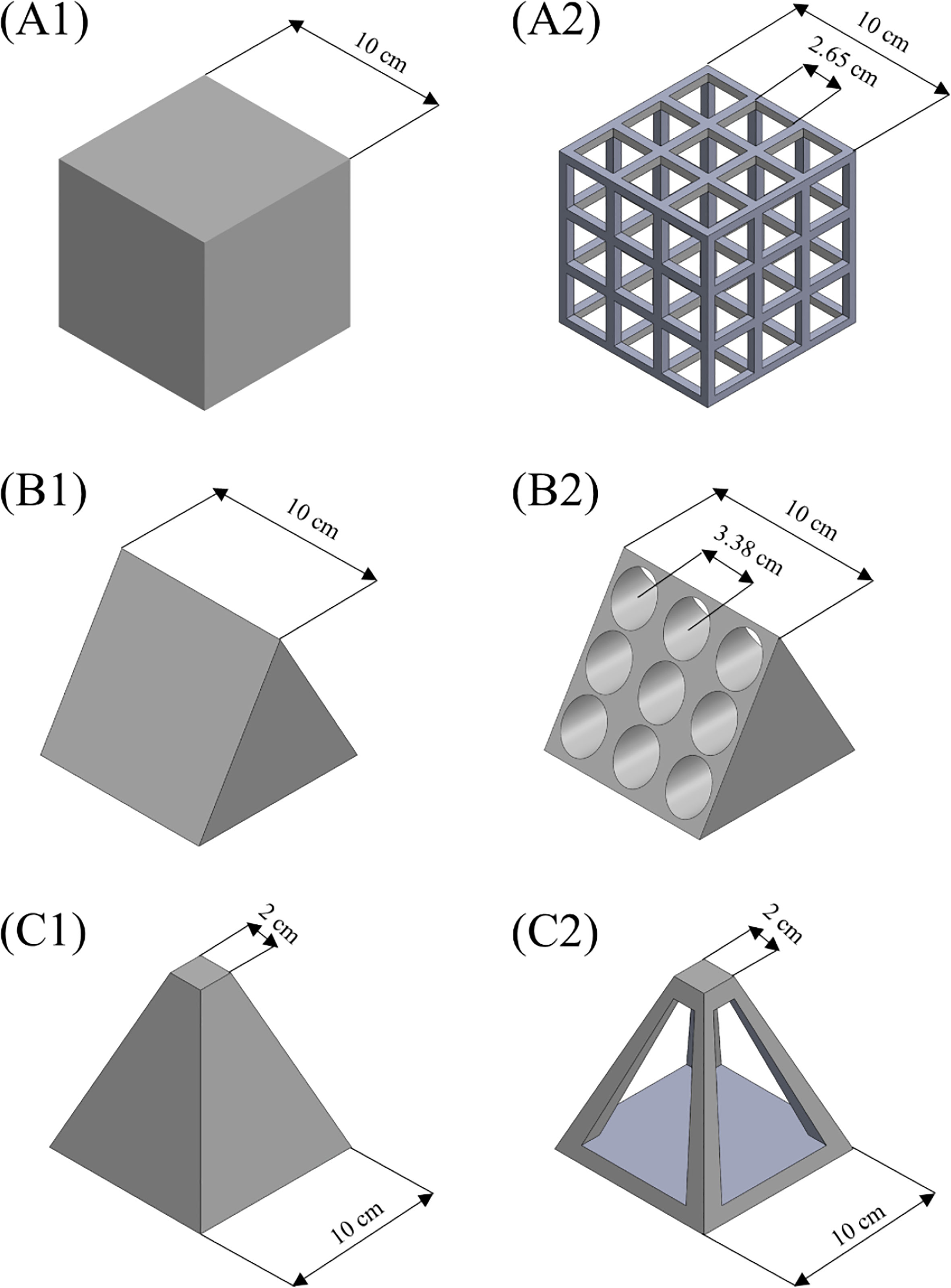
Figure 1 Six basic AR structure models; (A1) Solid cube; (A2) Hollow cube; (B1) Solid triangular pyramid; (B2) Hollow triangular pyramid; (C1) Solid truncated rectangular pyramid; (C2) Hollow truncated rectangular pyramid.
A computational domain of 1.60 m × 0.45 m × 0.60 m was set in the Cartesian coordinate system, whose origin was at the bottom center of the inlet boundary. The slope of the numerical flume was set to 0° because its actual slope ranged from 0° to 3°. The AR models were located 0.55 m downstream the inlet boundary and 0.225 m from both sides of the computational domain, which was divided into tetrahedral (pyramidal) unstructured grids. Grid independence was checked according to the method (Biron et al., 2004). When the calculation results of the different grid models are close to each other, it is believed that the simulated value is close to the actual value if the error of 90% of the flow field points is less than 5%. As a criterion for comparison, the maximum velocity was documented and compared among the cases, as summarized in Table 1. The test results tended to converge as the grid number increased. Based on the model with the densest grid case (total elements of 30 × 104), the model with a grid of 20 × 104 reached the requirements of grid independence. To balance the accuracy and efficiency of the model calculation, a model with a grid of 22 × 104 elements was applied in the numerical simulation (Figure 2).
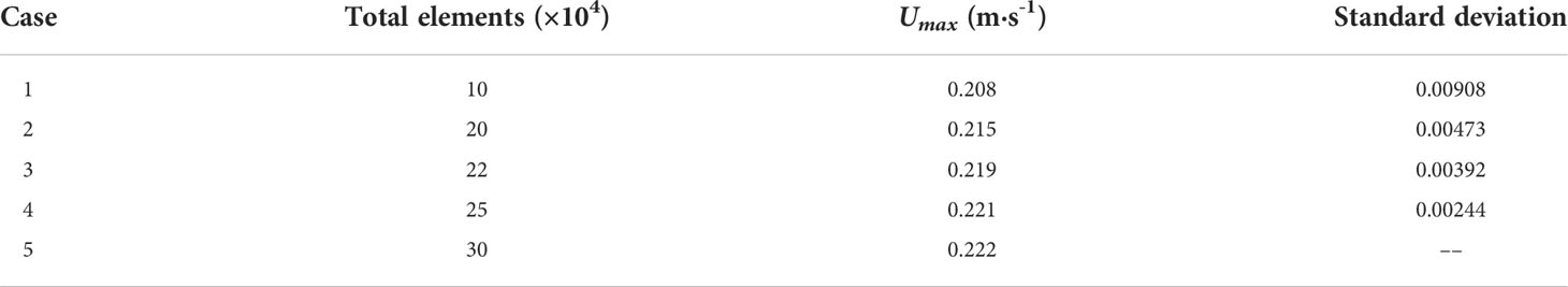
Table 1 Grid independence verification.
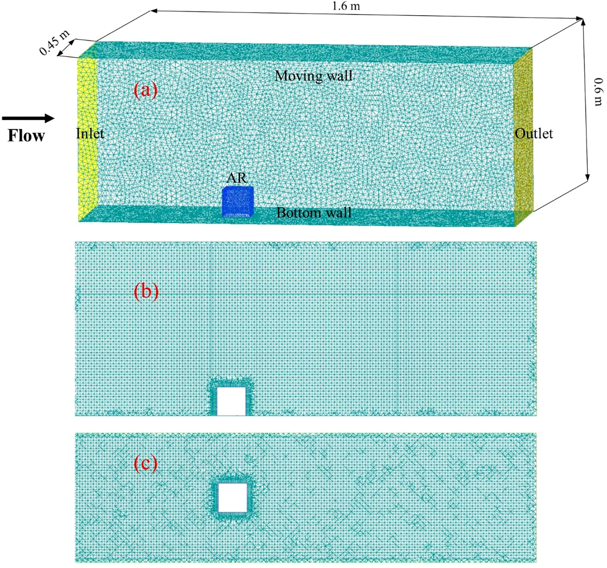
Figure 2 Schematic illustration of the grids in the computational domain; (A) 3D view; (B) Left view; (C) Top view.
The flow was set as an incompressible, steady, and viscous Newtonian fluid, and the boundary conditions for the solution were set as follows: To the left of the inlet, the average velocities were the same as those for the PIV experiments (0.067, 0.110, and 0.180 m/s), while the turbulence kinetic and dissipation rates were evaluated according to the computational formulas for the turbulence parameters (Table 2). In addition, the initial flow velocity, turbulent kinetic energy, and turbulent dissipation rate were set the same as the inlet boundary. The water flow at the right exit was considered as an outflow with unknown velocity and pressure values, calculated from the incoming flow. The upper boundary was defined as a moving wall with zero shear force and the same velocity as the incoming flow. The sidewalls of the flume and AR were established with a stationary no-slip wall boundary condition. Overall, the outflow flux was equal to the inflow flux.
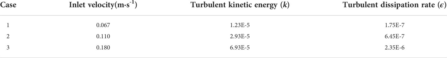
Table 2 Variable settings at the inlet.
In these simulations, the maximum Reynolds number is approximately 81,000, which implies that the resistance regime is transitional and not fully developed turbulence. Because the RNG k-ϵ turbulence model is a high Reynolds number model and is weak in the treatment of solid boundaries, the standard wall function (ANSYS Inc, 2016) was used for the near-wall turbulence treatment in this study, which is based on assumptions (Launder & Spalding, 1974). y+ is the dimensionless wall distance. The condition in Fluent for this method is that the y+ value be between 30 and 300, which is the intersection of the logarithmic and linear near-wall profiles. The y+ value was set to 40 in this study, and the height of the first layer of mesh nodes near the wall was 0.01 m. As AR is usually made of stone or concrete, the roughness height of the AR was set to 4 × 10⁻⁴ m according to a previous study (Jiang et al., 2021). The finite volume method (FVM) was used to disperse the governing equations. A 3D pressure-based solver and second-order implicit unsteady formulations were adopted. The least-squares cell-based method was used to calculate the gradients of the governing equations. SIMPLEC (SIMPLE-Consistent), an improved algorithm of semi-implicit method for pressure-linked equations (SIMPLE), was employed to iterate the equations (Van Doormaal and Raithby, 1984). A second upwind discretization scheme was used for the convection term of the momentum, turbulent kinetic energy, and energy dissipation rate equations. The solution convergence criterion was selected as 10−5 with a maximum of 30 iterations per time step.
1.2 Experimental validation
To validate the simulation results, laboratory experiments were conducted in an open-water recirculation channel at the State Key Laboratory of Coastal and Offshore Engineering, Dalian University of Technology, P. R. China. The basic test equipment included a rectangular flume and a high-speed PIV system.
1.2.1 AR model
The solid cubic AR model, shown in Figure 1 (A1), was used in the laboratory experiments. The dimensions of the AR model were 0.1 m × 0.1 m × 0.1 m (length × width × height). The AR model was scaled by a factor of 1:5 to satisfy the physical constraints of the flume measuring area and to avoid inducing an undesirable channel wall effect.
1.2.2 Experimental flume
The experimental flume was 22 m × 0.45 m × 0.6 m (length × width × height). The water depth of the test was 0.45 m, and the maximum test section was 0.45 m wide, 0.6 m deep and 1.6 m long. The sides and bottom of the test area at the center of the water channel were composed of glass to facilitate the PIV measurement of the flow fields at various positions around the AR model. A centrifugal pump was fixed to the left of the flume, which afforded flow velocities of 0.067 m/s, 0.11 m/s, and 0.18 m/s. The corresponding original physical values were 0.3 m/s, 0.5 m/s, and 0.8 m/s with full-scale reefs. The incoming velocity was measured using acoustic Doppler current velocimetry. The flume tank inflow was generated using a water pump. Water was drawn from the reservoir, injected at one end of the tank, and flowed to the other side. Moreover, the PIV calibration experiment was performed before the model experiments, and the results of the PIV measurement showed that the flow field in the experimental section was uniform. The inflow velocities were determined when the pump was used. With different inflow velocities, the difference in water depth was a few centimeters. This study focuses on the hydrodynamic performance of the boundary layer on the reef surface; therefore, the water depth difference is negligible.
1.2.3 PIV system
A schematic layout of the experimental arrangement is shown in Figure 3. The basic optical devices of the PIV system were designed according to the experimental configuration specified by TSI, Inc. (USA). Reflective polyvinyl chloride powder with a mean diameter of 10 μm and a density of 1050 kg/m3 was added to the water as a trace particle. The light sheets were generated by an Nd: YAG laser capable of producing 3–5 ns, 120 mJ pulses at a repetition frequency of 15 Hz. Digital images were captured using a high-resolution CCD camera with two million pixels. The maximum frame rate of the camera was 32 f/s. To acquire images, a CCD camera (Power View 4 MP) coupled to the PC image acquisition software was used. The operation of the laser and camera was synchronized with a digital delay pulse generator. These images were processed using a window size of 32×32 pixels, with a 32-pixel analysis step. The calculation of the speed of the particles in the raw particle images was based on cross-correlation, and techniques such as erroneous vector correction were employed to reduce the computing error. The velocity distribution vector data around the artificial reef were acquired by performing the established procedures. The flow-field data were determined as the average value of 15 pairs of instantaneous flow fields.

Figure 3 A schematic illustration of the experimental apparatus and the PIV system.
1.3 A method for evaluating the flow field effect of ARs
To quantitatively compare the flow-field effects of ARs with different structures, an evaluation method was developed.
1.3.1 Selection of evaluation indices
To develop the evaluation method, the first step is to select the evaluation indices. Previous studies discussed above have established that different flow field characteristics around ARs can support ecological service functions, such as promoting the transportation and exchange of nutrients, increasing the diffusion of bait organisms, and improving the natural habitat (Jiang et al., 2016; Perkol-Finkel et al., 2018; Kim et al., 2019; Li et al., 2021; Zheng et al., 2022). To fully evaluate the flow field effects of ARs, the evaluation indices were selected by referring to these studies, as shown in Table 3. The evaluation index definitions of upwelling and back vortex flow are based on previous studies, and the definitions of other evaluation indices are defined herein.
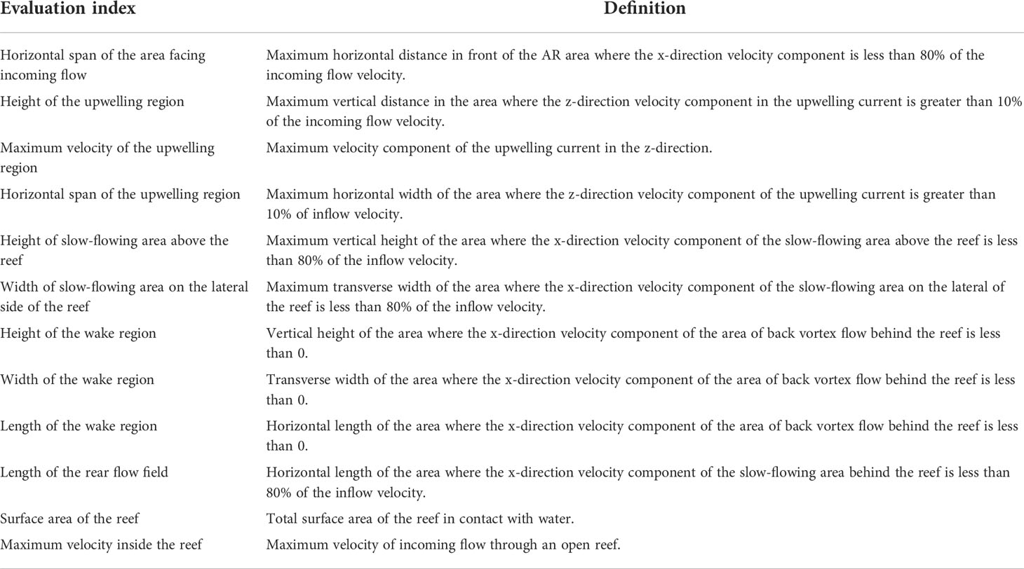
Table 3 Evaluation indices and definitions of the flow field effect of ARs.
The analytic hierarchy process (AHP) approach has been extensively used in environmental and safety sciences (Lyu et al., 2020; Hu et al., 2021). The AHP approach is a decision-making method that decomposes decision indices into three levels: objectives, criteria, and options. Subsequently, qualitative and quantitative analyses are performed (Lee, 2015). In this study, this approach was applied to establish an evaluation model based on the flow field effect of ARs. The specific process is as follows: After determining the evaluation indices, the evaluation model was divided into three levels. The flow field effect of the ARs was set as the objective level. Six preliminary evaluation indices, including upwelling region, wake region, surface area of ARs, upper slow-flowing area, lateral slow-flowing area, and internal velocity of ARs, were set as the criteria level. Twelve specific evaluation indices belonging to the preliminary indices were set as option levels (Figure 4).
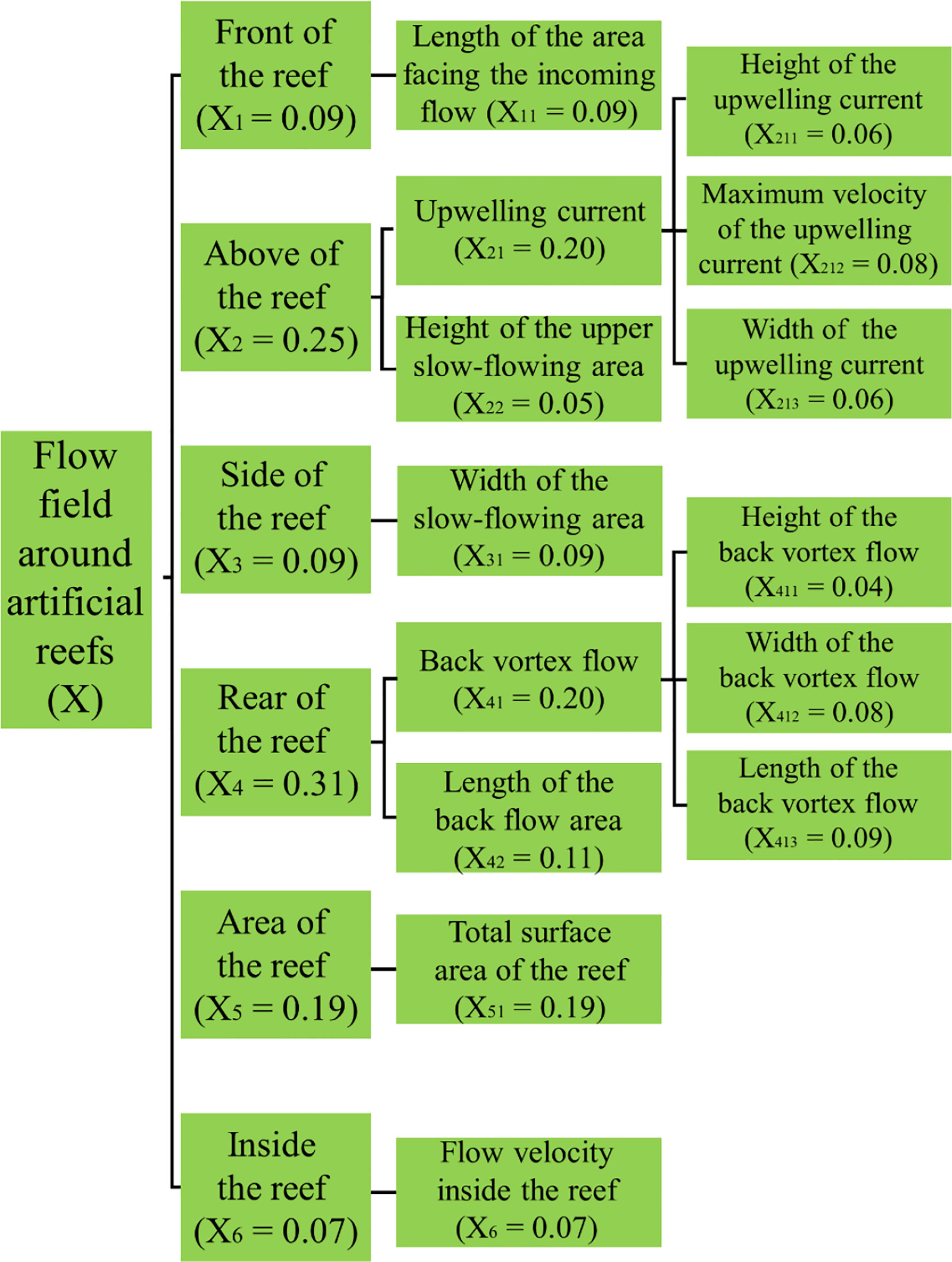
Figure 4 Evaluation model of the flow field effect of ARs and the weights of evaluation indices in the model.
The AHP approach calculates the weight of each index by comparing the relative importance (contribution to the objective) of each of the two indices, which is relatively subjective. The entropy weight method (EWM) was used in this study to objectively determine each index. EWM is based on information theory, in which information entropy is a measure of the degree of disorder in a system, and it can be used to determine the dispersion degree of a certain index. The smaller information entropy value of an index indicates the greater the dispersion and influence (weight) of the index on the overall evaluation, and vice versa (Xiao, 2020). For example, if the difference in the upwelling is greater than that of the back vortex flow in the simulation results across all AR structures, the information entropy value of the upwelling is smaller than that of the back vortex flow, and the weight of the upwelling is larger than that of the back vortex flow. Determining the weights based on the EWM comprises three steps: In the first step, the original data matrix X was formed (Eq. 6), where m is the evaluation index of the flow field effect (e.g., upwelling), and n is the evaluation object (flow field simulation results with different ARs). Next, matrix X was normalized (Eq. 7), where rij is the standard value of the j evaluation object on i evaluation index. The rij value was calculated using Eq. 8, and it ranged from 0 to 1. In the second step, the entropy of i evaluation index was calculated using Eq. 9, where fij and k are defined as follows (Eq.10–11): In the third step, the entropy weight of the i evaluation index was calculated using Eq.12, where wi ranges from 0 to 1 (Eq. 13). The weights of each index are shown in Figure 4.
2 Result and discussion
2.1 Comparison of simulation and experiment results
Figure 5 shows a comparison of the simulation and experimental results of the velocity distribution around the solid cubic reef. The velocity distribution in the simulation was fundamentally consistent with that in the experiment. A comparison of the intensities and scale of the upwelling and back vortex flow between the simulation and experiments is shown in Figure 6. The relative errors of the height and width of the upwelling current between the simulation and experimental results were 2.8%–12.23% and 7.92%–10.1%, respectively, and the relative errors of the height and length of the back vortex flow were 7.8%–13.42% and 8.86%–10.85%, respectively. The mean error between the simulation and experimental values was 8.78%, which was less than 10%. The simulation results were in good agreement with the experimental results, and the numerical model demonstrated high accuracy. Therefore, the flow fields of other AR structures can be accurately simulated by the numerical model, which provides a basis for evaluating the flow-field effects of ARs.
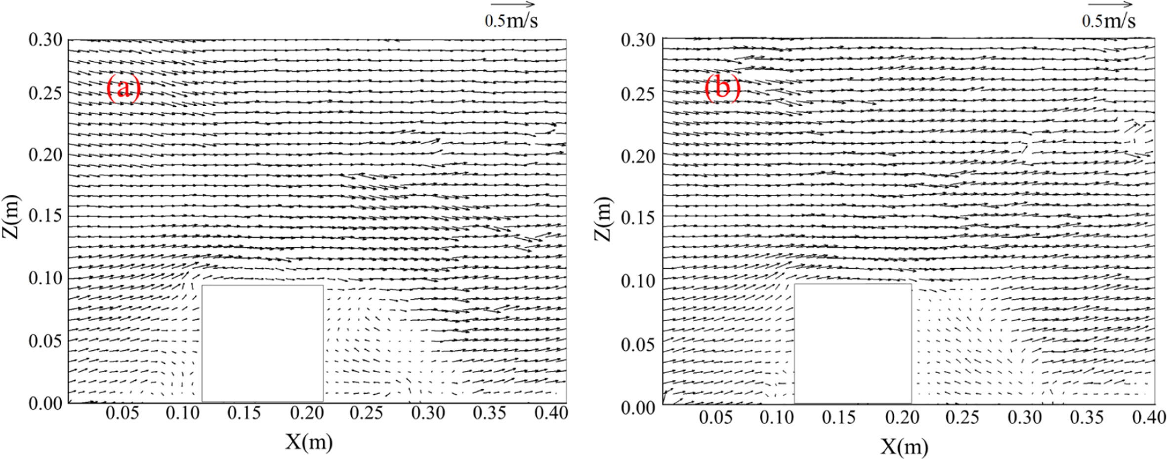
Figure 5 Flow field diagram of (A) Fluent simulation and (B) PIV experiment for solid cubic AR at a velocity of 0.18 m/s.
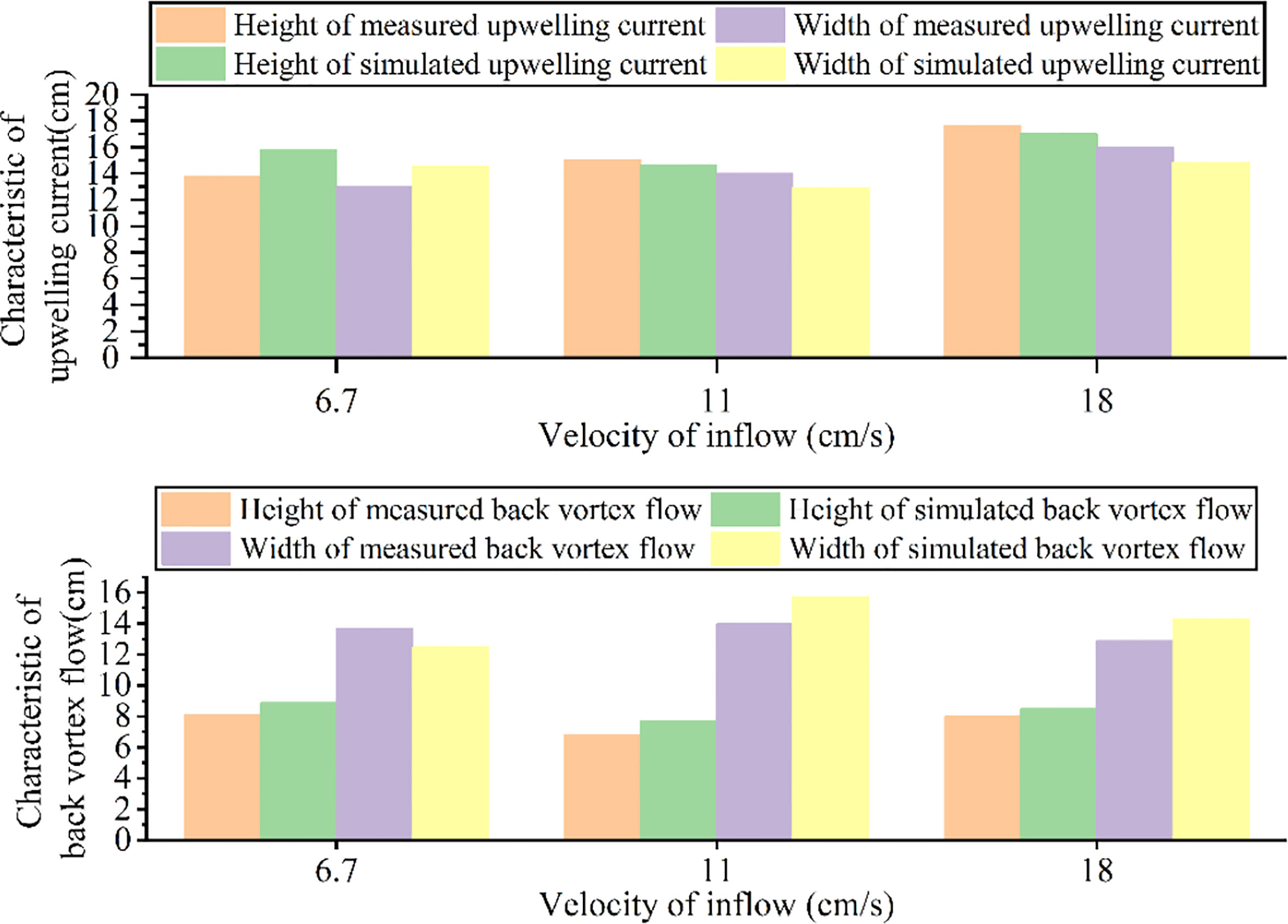
Figure 6 Heights and widths of upwelling and the heights and widths of back vortex flow of solid cubic AR at three velocities.
2.2 Flow fields of ARs with six basic structures
The velocity contours of the flow fields of the ARs with six basic structures at an s incoming velocity of 0.18 m/are shown in Figure 6, which shows the x-z plane (y = 0) in the Cartesian coordinate system. Apparently, compared to the horizontal span of the area facing the incoming flow, A2 was close to A1, but B2 was smaller than B1 and C2 was much smaller than B3. The results suggest that excessive opening holes are disadvantageous in the formation of slow-flowing areas facing the incoming flow. From the respective upwelling, the upwelling heights and widths of the solid ARs (A1, B1, and C1) were higher than those of the hollow ARs (A2, B2, and C2), while the maximum velocities of the solid and hollow ARs were close. The results indicate that in these basic AR structures, solid ARs have better upwelling indices than hollow ARs. From the back vortex flow perspective, the heights and widths of the back vortex flow in A1 and B1 were similar, while B2 was smaller than B1, and C2 was much smaller than B3. The results indicate that an excessive opening hole was not beneficial in the formation of a back vortex flow. Streamline diagrams of the flow fields of the ARs with six basic structures at an incoming velocity of 0.18 m/s are shown in Figure 7, which is in the same plane as Figure 6. For solid ARs (A1, A2, A3), the location of the back vortex center of the flow field around different ARs was different. For the hollow ARs, only B1 had a back-vortex center. These results show that the back-vortex flow is strongly influenced by the AR structure, and an excessive opening hole inhibits its formation. As shown in Figures 7 and 8, A1 has a better upwelling index, and A2 has a better back-vortex flow index. Therefore, ARs with better flow-field effects must be determined using the evaluation method.
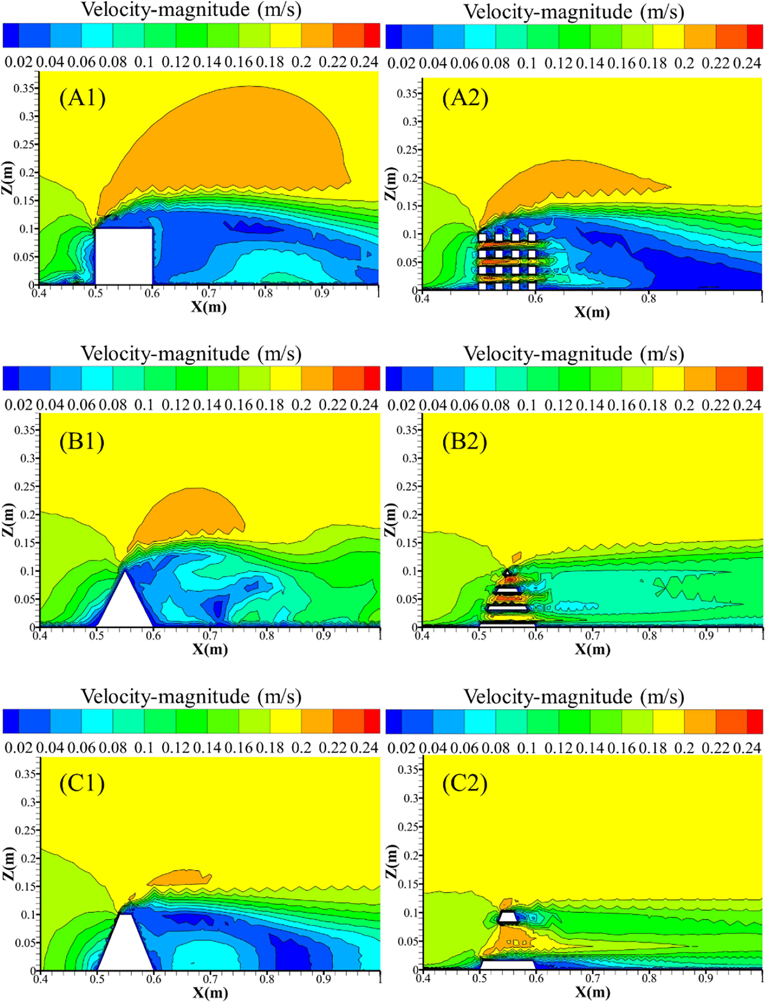
Figure 7 Velocity contours of the flow fields of ARs with six basic structures; (A1) Solid cube; (A2) Hollow cube; (B1) Solid triangular pyramid; (B2) Hollow triangular pyramid; (C1) Solid truncated rectangular pyramid; (C2) Hollow truncated rectangular pyramid.
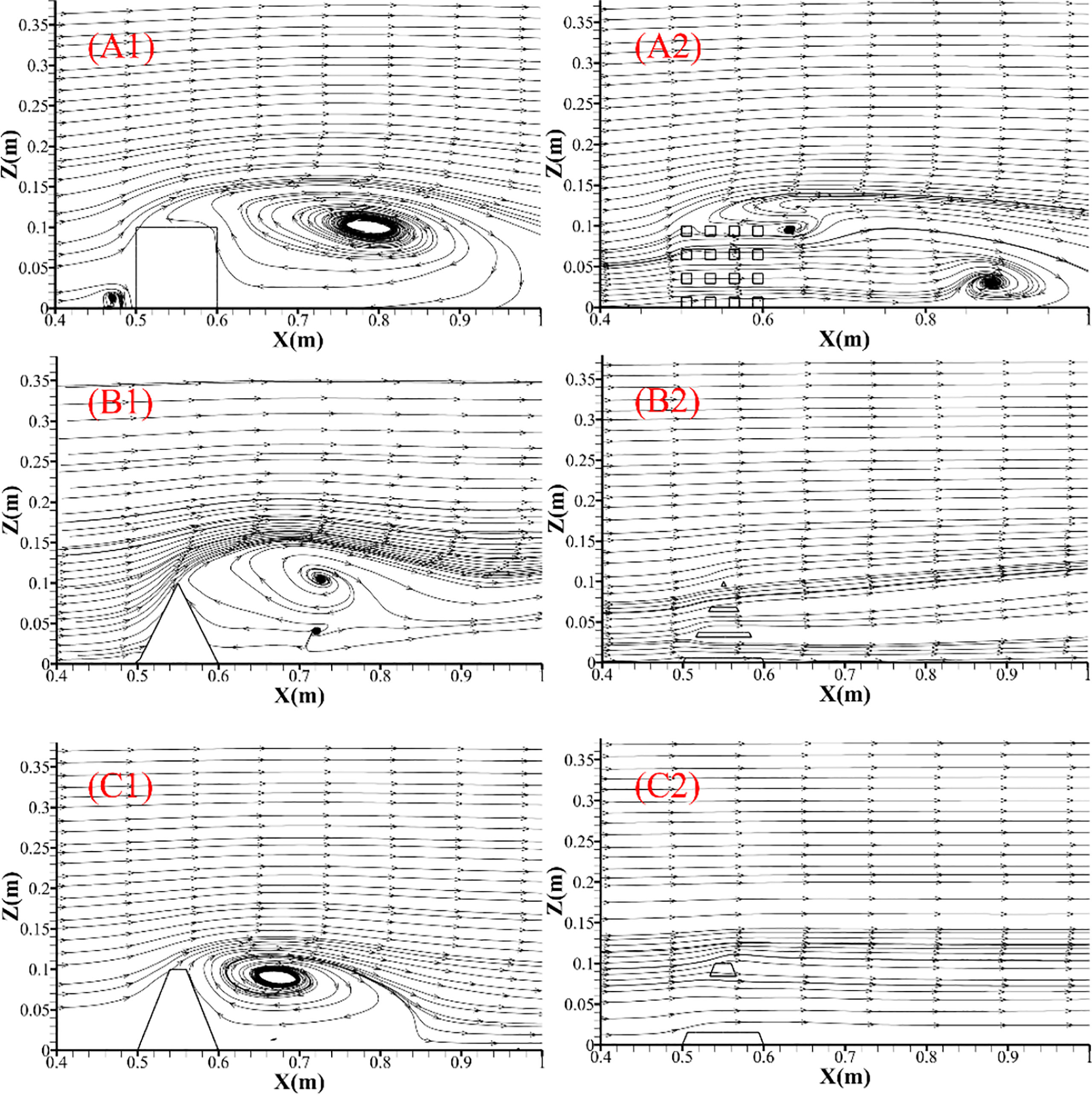
Figure 8 Streamline diagrams of the flow fields of ARs with six basic structures; (A1) Solid cube; (A2) Hollow cube; (B1) Solid triangular pyramid; (B2) Hollow triangular pyramid; (C1) Solid truncated rectangular pyramid; (C2) Hollow truncated rectangular pyramid.
2.3 Fuzzy comprehensive evaluation of the flow field effects of ARs with six basic structures
The flow-field effects of ARs with six basic structures were evaluated using the evaluation method proposed in this paper, as follows: First, based on the simulation results and the evaluation method we established, the eigenvalues and weights of each flow-field effect index of ARs with six basic structures after normalization were presented (Table 4). Next, based on the FCE method, Euclidean distances were calculated and were used to judge the superiority of AR with j structure (Eq.14–15), where rij and wi were calculated using Eq. 8 and Eq. 12. Eventually, the relative superiority (Uj) of the AR with j structure was determined (Eq. 16). The superiority of the flow-field effect of ARs can be determined by comparing Uj (Table 5). In the ARs with the six basic structures used in this study, the ranking of their flow field effects from best to worst was A2, A1, B1, C1, B2, and C2. One unanticipated finding was that the hollow AR (A2) with open holes had a better flow field effect than the solid AR (A1). These results corroborated the findings of a several previous studies (Wang et al., 2018; Tang et al., 2019; Nie et al., 2022), demonstrating that opening holes has a significant influence on the flow field of AR. Wang’s study suggested that the flow effect of AR can be improved by the appropriate cut-opening ratio (OR), especially back vortex flow. A proper increase in the OR of a cubic reef was beneficial to expand the range of back eddies in the flow field. In Figure 8, the back eddy current range of A2 was significantly larger than that of A1, which was in a good agreement with Wang’s study. According to Tang’s and Nie’s studies, excessive OR might cause enhanced permeability of a cubic artificial reef, resulting in an obvious reduction of upwelling and back vortex flow at a high-level of OR. This was consistent with the simulation results of A2 and A3 in this study. When the OR was too large, the upwelling and back vortex flow was greatly reduced. In addition, this ranking was consistent with the flow-field simulation results for each AR structure. A1 and A2 demonstrated better upwelling and back vortex flow indices than the other four structures (Figure 7), so A1 and A2 ranked in the front. B2 and C2 did not have back-vortex flow formation, and the flow field effects were evidently worse than those of the other four structures (Figure 7), so B2 and C2 ranked behind.
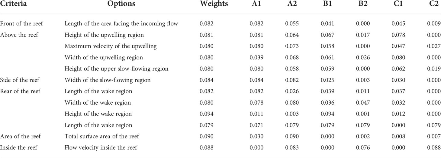
Table 4 Eigenvalues and weights of each flow-field effect index of the ARs with six basic structures after normalization.
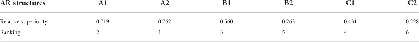
Table 5 Superiority ranking of the flow-field effect of ARs with six basic structures.
3 Conclusion
Previous studies have evaluated the flow field effects of ARs using a single index, such as upwelling and back-vortex flow. However, quantitative studies on the flow-field effects of ARs have not been conducted. Herein, the flow fields of the ARs with six basic structures were simulated and validated using PIV flume experiments. An evaluation method was proposed and applied to the flow-field ARs with six basic structures based on the simulation results. The conclusions are as follows:
First, based on computational fluid dynamics (CFD), a numerical model was established to simulate the flow fields of ARs with six basic structures. For the solid cubic AR, the simulation flow field was consistent with the PIV experimental flow field. The average error of the flow field effect indices (upwelling and back vortex flow) between the simulation and experimental results was 8.78%. Hence, the numerical model demonstrated high accuracy and can be used as a reference for the flow-field effect of ARs.
Second, for the first time, an evaluation method to quantitatively analyze the flow-field effect of AR was proposed. According to the present study, more flow field indices (upwelling region, wake region, surface area of ARs, upper slow-flowing area, lateral slow-flowing area, and internal velocity of ARs) were identified for evaluation. The evaluation indices were divided into three levels (objectives, criteria, and options) based on the AHP approach. The weights of the evaluation indices were objectively determined by the EWM. The evaluation method that combines AHP and EWM makes the evaluation results more systematic and objective.
Third, the evaluation method was used to evaluate the flow fields of ARs with six basic structures based on the simulation results. The superiority of the ARs was calculated and ranked based on FCE. The ranking results were in accordance with the simulation results in several ways. Therefore, the evaluation method has a certain degree of accuracy in the evaluation of the flow field effect of ARs and can provide the basis for the structure selection and optimization of ARs.
The aim of this study was to preliminarily establish an evaluation method for quantitatively evaluating the flow field effect of AR. A limitation of this study is that the studied structures of ARs are basic and some of them are not widely applied. Further studies evaluating more widely used AR structures will be conducted in the future.
Data availability statement
The original contributions presented in the study are included in the article/supplementary material. Further inquiries can be directed to the corresponding authors.
Author contributions
QM: Methodology and Writing – original draft. JD: Investigation and Data curation – review and editing. YX: Formal analysis and Visualization. JS: Resources and Project administration. SL: Conceptualization and Funding acquisition RZ: Supervision and Funding acquisition. All authors contributed to the article and approved the submitted version.
Funding
The work was funded by the National Key R&D Program of China [Grant No. 2019YFC1407700], the National Natural Science Foundation of China [Grant No. 31302232 and Grant No. 51779038], the Key Laboratory of Environment Controlled Aquaculture, Ministry of Education of China [2021-MOEKLECA-KF-06].
Acknowledgments
We thank the Data Support from National Marine Scientific Data Center (Dalian), National Science & Technology Infrastructure of China (http://odc.dlou.edu.cn/) for providing valuable data and information. We also thank the reviewers for carefully reviewing the manuscript and providing valuable comments to help improve this paper.
Conflict of interest
The authors declare that the research was conducted in the absence of any commercial or financial relationships that could be construed as a potential conflict of interest.
Publisher’s note
All claims expressed in this article are solely those of the authors and do not necessarily represent those of their affiliated organizations, or those of the publisher, the editors and the reviewers. Any product that may be evaluated in this article, or claim that may be made by its manufacturer, is not guaranteed or endorsed by the publisher.
References
Biron M. P., Ramamurthy S. A., Han S. (2004). Three-dimensional numerical modeling of mixing at river confluences. J. Hydraul. Eng. 130 (3), 243–253. doi: 10.1061/(ASCE)0733-9429(2004)130:3(243)
Chang C. Y., Schmidt J., Dörenkämper M., Stoevesandt B. (2018). A consistent steady state CFD simulation method for stratified atmospheric boundary layer flows. J. Wind Eng. Ind. Aerod. 172, 55–67. doi: 10.1016/j.jweia.2017.10.003
Feng Q., Sun T. (2020). Comprehensive evaluation of benefits from environmental investment: Take China as an example. Environ. Sci. pollut. R. 27 (13), 15292–15304. doi: 10.1007/s11356-020-08033-7
Folpp H. R., Schilling H. T., Clark G. F., Lowry M. B., Maslen B., Gregson M., et al. (2020). Artificial reefs increase fish abundance in habitat-limited estuaries. J. Appl. Ecol. 57 (9), 1752–1761. doi: 10.1111/1365-2664.13666
Hu X. J., Ma C. M., Huang P., Guo X. (2021). Ecological vulnerability assessment based on AHP-PSR method and analysis of its single parameter sensitivity and spatial autocorrelation for ecological protection? A case of weifang city, China. Ecol. Indic. 125, 107464. doi: 10.1016/j.ecolind.2021.107464
Ihsan K., Murat C., Fulya T. (2019). A comprehensive review of fuzzy multi criteria decision making methodologies for energy policy making. Energy Strateg. Rev. 24, 207–228. doi: 10.1016/j.esr.2019.03.003
Jiang Z. Y., Lin N., Yuan X. W., Jiao H. F., Shentu J. K., Li S. F. (2016). Effects of an artificial reef system on demersal nekton assemblages in Xiangshan Bay, China. Chin. J. Oceanol. Limn. 34 (1), 59–68.
Jiang Z. Y., Liang Z. L., Zhu L. X., Guo Z. S., Tang Y. L. (2020). Effect of hole diameter of rotary-shaped artificial reef on flow field. Ocean. Eng. 197, 106917. doi: 10.1016/j.oceaneng.2020.106917
Jiang Z. Y., Zhu L. X., Mei J. X., Guo Z. S., Cong W., Liang Z. L. (2021). Preliminary study on the boundary layer of an artificial reef with regular grooves surface structure. Ocean. Eng. 219 (1), 108355. doi: 10.1016/j.oceaneng.2020.108355
Kim D., Jung S., Kim J., Na. W. B. (2019). Efficiency and unit propagation indices to characterize wake volumes of marine forest artificial reefs established by flatly distributed placement models. Ocean Eng. 175, 138–148. doi: 10.1016/j.oceaneng.2019.02.020
Launder E., Spalding D. B. (1974). The numerical computation of turbulent flows. Comput. Methods Appl. Math. 3, 269–289. doi: 10.1016/0045-7825(74)90029-2
Lee S. (2015). Determination of priority weights under multiattribute decision-making situations: AHP versus fuzzy AHP. J. Constr. Eng. M. 141 (2), 05014015. doi: 10.1061/(ASCE)CO.1943-7862.0000897
Li J. J., Li J., Gong P. H., Guan C. T. (2021). Effects of the artificial reef and flow field environment on the habitat selection behavior of sebastes schlegelii juveniles. Appl. Anim. Behav. Sci. 245, 105492. doi: 10.1016/j.applanim.2021.105492
Li J., Zheng Y. X., Gong P. H., Guan C. T. (2017). Numerical simulation and PIV experimental study of the effect of flow fields around tube artificial reefs. Ocean. Eng. 134, 96104. doi: 10.1016/j.oceaneng.2017.02.016
Liu T. L., Su D. T. (2013). Numerical analysis of the influence of reef arrangements on artificial reef flow fields. Ocean. Eng. 74, 81–89.
Lyu H. M., Zhou W. H., Shen S. L., Zhou A. N. (2020). Inundation risk assessment of metro system using AHP and TFN-AHP in shenzhen. Sustain. Cities Soc. 56, 102103. doi: 10.1016/j.scs.2020.102103
Nie Z. Y., Zhu L. X., Xie W. D., Zhang J. T., Wang J. H., Jiang Z. Y., et al. (2022). Research on the influence of cut-opening factors on flow field effect of artificial reef. Ocean. Eng. 249, 110890. doi: 10.1016/j.oceaneng.2022.110890
Perkol-Finkel S., Hadary T., Rella A., Shirazi R., Sella I. (2018). Seascape architecture – incorporating ecological considerations in design of coastal and marine infrastructure. Ecol. Eng. 120, 645–654. doi: 10.1016/j.ecoleng.2017.06.051
Roughan M., Cetina-Heredia P., Ribbat N., Suthers I. M. (2022). Shelf transport pathways adjacent to the East Australian current reveal sources of productivity for coastal reefs. Front. Mar. Sci. 8, 789687.
Tang Y. L., Yang W. Z., Sun L. Y., Zhao F. F., Long X. Y., Wang G. (2019). Studies on factors influencing hydrodynamic characteristics of plates used in artificial reefs. J. Ocean. U. China. 18 (1), 193–202. doi: 10.1007/s11802-019-3706-z
Taormina B., Claquin P., Vivier B., Navon M., Pezy J. P., Raoux A., et al. (2022). A review of methods and indicators used to evaluate the ecological modifications generated by artificial structures on marine ecosystems. J. Environ. Manage. 310, 114646. doi: 10.1016/j.jenvman.2022.114646
Van Doormaal J. P., Raithby G. D. (1984). Enhancements of the SIMPLE method for predicting incompressible fluid flows. Numer. Heat. Tr. 7 (2), 147–163. doi: 10.1080/10407798408546946
Wang X. L., Wang X., Zhu J. F., Li F., Li Q. S., Che H. (2017). A hybrid fuzzy method for performance evaluation of fusion algorithms for integrated navigation system. Aerosp. Sci. Technol. 69, 226–235. doi: 10.1016/j.ast.2017.06.027
Wang G., Wan R., Wang X. X., Zhao F. F., Lan X. Z., Cheng H., et al. (2018). Study on the influence of cut-opening ratio, cut-opening shape, and cut-opening number on the flow field of a cubic artificial reef. Ocean. Eng. 162, 341–352. doi: 10.1016/j.oceaneng.2018.05.007
Xiao F. Y. (2020). EFMCDM: Evidential fuzzy multicriteria decision making based on belief entropy. IEEE T. Fuzzy. Syst. 28 (7), 1477–1491. doi: 10.1109/TFUZZ.2019.2936368
Yakhot V., Orszag S. A. (1986). Renormalization group analysis of turbulence: basic theory. J. Sci. Comput. 1 (1), 3–11. doi: 10.1007/BF01061452
Yakhot V., Orszag S. A., Thangam S., Gatski T. B., Speziale C. G. (1992). Development of turbulence models for shear flows by a double expansion technique. Phys. Fluids. A. 4 (7), 1510–1520. doi: 10.1063/1.858424
Keywords: artificial reef, PIV flume experiment, numerical simulation, flow field, fuzzy comprehensive evaluation
Citation: Ma Q, Ding J, Xi Y, Song J, Liang S and Zhang R (2022) An evaluation method for determining the optimal structure of artificial reefs based on their flow field effects. Front. Mar. Sci. 9:962821. doi: 10.3389/fmars.2022.962821
Received: 06 June 2022; Accepted: 06 September 2022;
Published: 23 September 2022.
Edited by:
Won-Bae Na, Pukyong National University, South KoreaCopyright © 2022 Ma, Ding, Xi, Song, Liang and Zhang. This is an open-access article distributed under the terms of the Creative Commons Attribution License (CC BY). The use, distribution or reproduction in other forums is permitted, provided the original author(s) and the copyright owner(s) are credited and that the original publication in this journal is cited, in accordance with accepted academic practice. No use, distribution or reproduction is permitted which does not comply with these terms.
*Correspondence: Shuxiu Liang, c3hsaWFuZ0BkbHV0LmVkdS5jbg==; Ruijin Zhang, cnVpamluekBkbG91LmVkdS5jbg==