 Bin Deng
 Wen Zhang
 Yu Yao
 Changbo Jiang
- 1School of Hydraulic and Environmental Engineering, Changsha University of Science and Technology, Changsha, China
- 2Key Laboratory of Water-Sediment Sciences and Water Disaster Prevention of Hunan Province, Changsha University of Science and Technology, Changsha, China
Swash zone hydrodynamics has significant coastal geomorphological and engineering implications. However, there is still a research gap in fully understanding the response of bore-driven swash hydrodynamics to varying beach slopes. Therefore, in this study, laboratory experiments were performed in a flume to investigate the hydrodynamics of bore-driven swash flows over impermeable smooth beaches with a mild slope (1:35), a steep slope (1:10), and a composite slope (1:35–1:10), respectively. The designed swash events are produced by a collapse of dam-break-generated bores. Wave gauges, ultrasonic displacement sensors, acoustic Doppler velocimeter, and particle image velocimetry are used simultaneously to capture different phases (bore collapse, uprush, and backwash) of bore evolution in the entire swash zone. The impacts of beach slope on the swash hydrodynamics in view of the shoreline movement, swash depth, and swash velocity are first analyzed. The formation and evolution of the vortex structure on the three beaches are also reported in this study.
1 Introduction
When the waves reach the shoreline, the beach area is alternately covered and uncovered by water. The area between the maximum runup and rundown of waves is known as the swash zone, where multiple dynamic processes occur (Zhu and Dodd, 2020). The flow in this area presents high speed, high transient, violent aeration, and non-uniform characteristics, which play an important role in wave structure interaction, sediment transport, and morphological dynamics (Zhang and Liu, 2008). In laboratory studies, the isolation of such processes occurs for a single swash event via solitary wave, dam-break forcing, or ensemble averaging of swash events under regular or irregular wave forcing (Chardón-Maldonado et al., 2016). The bore-generated swash propagation on a sloping beach has been studied by many researchers for a long time (Mory et al., 2011). Bore-driven swash hydrodynamics usually includes three successive stages: bore collapse [collapse at the still water level (SWL), propagation near the shoreline] (Yeh et al., 1989), uprush (when water climbs the beach to a maximum runup), and backwash (when the water reversely moves to the farthest position from the beach, where it encounters the next arriving bore) (Alsina and Cáceres, 2011).
In the past two decades, efforts have been made to study hydrodynamics within the swash zone by using single swash events generated by dam-break bores in the laboratory. Yeh et al. (1989) first carried out experiments based on the mechanism of dam break to study the bore propagation over a uniformly sloping beach. Barnes et al. (2009) measured the bed shear stress using a shear plate in the laboratory bore-driven swash. Moreover, O’Donoghue et al. (2010) conducted laboratory experiments and provided comprehensive detailed measurements of the swash hydrodynamics, including flow depth, velocity, and turbulence. Meanwhile, Sou et al. (2010) and Sou and Yeh (2011) studied how turbulence evolved during swash motion using laboratory PIV measurements. Recently, the hydrodynamics of swash zone has been further researched: Chen et al. (2016) obtained the detailed hydrodynamics of swash–swash interactions by experimental measurement, and Van der Zanden et al. (2019) carried out a laboratory experiment to generate two continuously alternating swash events and obtained the sand transport processes and bed level changes within the two alternating swash events. Bergsma et al. (2019) carried out experimental measurements to analyze the hydrodynamic parameters at the collapse point and investigated the link between broken wave properties at bore collapse and wave runup. Recent studies have alternatively established numerical models to describe the hydrodynamic process (e.g., Guard and Baldock, 2007; Puleo et al., 2007; Kelly and Dodd, 2010; Mory et al., 2011; Deng et al., 2012; Jiang et al., 2013; Briganti et al., 2016; Hammeken and Simons, 2017; Kim et al., 2017; Aboulatta et al., 2020; Wu et al., 2020). The abovementioned studies show that successful efforts have been made to measure and simulate the hydrodynamics of swash flow, and these studies have provided us with an improved understanding of the hydrodynamic characteristics of the swash zone.
The flow characteristics in the swash zone are unique because of continuously varying shallow water depth and inundation intermittency. Jaffe and Rubin (1996) and Cox and Kobayashi (2000) showed that sediment transport in the swash zone is related to the intermittence of turbulence. The generation and evolution of turbulent coherent structure and its impact on the beach may be different at different stages of the swash (Puleo et al., 2000; Butt et al., 2004; Alsina et al., 2009; Alsina and Cáceres, 2011). In existing research, understanding swash zone hydrodynamics is challenging due to difficulties in measuring the structure of the highly transient and irregular turbulent flow. Meanwhile, the RANS model cannot resolve the turbulence directly, especially the role of turbulent coherent structure, vortex shape, and their dynamics in swash processes. Hence, quantifying the detailed flow characteristics and studying the evolution process of swash are needed to improve our knowledge of swash zone hydrodynamics.
However, the detailed flow structures in the swash zones have not been fully understood. As we all know, it is difficult to measure the swash flow details directly. One reason for the lack of flow details is the limitations of experimental equipment and measurement technology (Brocchini and Baldock, 2008). Most existing experimental studies used instruments such as pressure sensors (e.g., Masselink and Russell, 2006), capacitance-type wave gauges (e.g., O’Donoghue et al., 2010), laser Doppler velocimeters (e.g., Cox and Anderson, 2001; Petti and Longo, 2001), ultrasonic altimeters (e.g., Turner et al., 2008; Masselink et al., 2009), particle image velocimetry (e.g., O’Donoghue et al., 2010; Kikkert et al., 2012), and laser-induced fluorescence (e.g., Steenhauer et al., 2012; Kikkert et al., 2012) to conduct the measurements. Another reason comes from the fact that the flows are complicated, which are featured with strong aeration, high transient, large sediment transport rates, and rapid morphological changes (Aagaard and Hughes, 2006; Masselink and Russell, 2006; Othman et al., 2014; Chardón-Maldonado et al., 2016; O’Donoghue et al., 2016; Van der Zanden et al., 2019; Hu et al., 2020). In addition to the above reasons, the limitations of the study area also hinder a further understanding of the water flow in the swash zone. Previous studies have paid more attention to the hydrodynamic properties of the lower swash zone, and the arrangement of the experimental device did not even involve the upper swash zone (Sou et al., 2010). Moreover, the velocity, depth, and violent aerated thin-film flow in the middle and upper swash zones cannot be measured.
In addition, the type of beach is an important factor to control hydrodynamics with the swash zone (Miles et al., 2006). According to the classification proposed by Wright and Short (1984), beaches can be categorized into three: reflective beaches (steep beaches with narrow swash zones), dissipative beaches (mild beaches with wide swash zones), and intermediate beaches (beaches with a combination of the features of the other two beaches). Beach slope, to some extent, determines the type of wave breaking, thus the subsequent swash motions on the beach. For example, beach slope affected the energy during swash propagation. On steeper beaches where incident waves are not saturated, incident wave energy propagates more freely to the shoreline and contributes more energy to the spectrum in the inner surf zone. On steep beaches, incident waves may combine with reflected waves to transform energy to subharmonic frequencies (Miles et al., 2006). Beach slope also affected the runup during wave propagation. Ebrahimi et al. (2015) showed that the runup level is directly correlated to the beach slope.
However, most existing laboratory experiments were conducted on beaches with mild uniform slopes. In fact, experimental measurements on mild slopes can minimize the effects of air entrainment on imaging techniques (Shin and Cox, 2006). Sou et al. (2010) studied the evolution of the swash turbulence structure on a 1:20 slope glass beach, and Ting and Kirby (1994) , Cox and Anderson (2001), and Bakhtyar et al. (2009) carried out laboratory measurements on a plane 1:35 slope. However, protected beaches could have steeper slopes in the swash zone due to the presence of revetments. Therefore, some studies have focused on steep slopes, e.g., slope of 1:10 (Barnes et al., 2009; Kikkert et al., 2012; Kikkert et al., 2013; O’Donoghue et al, 2010) and 1:15 (Van der Zanden et al., 2019). In addition, in the field observation by Butt et al. (2004), the average beach slope during measurements was 0.108 (1:9.26). In summary, 1:10 is the most commonly used slope and 1:35 is the gentlest slope used in previous hydrodynamic studies. Many natural tidal beaches exhibit a steep upper section and a flat low tide section. However, in existing research, very few investigations on swash zones have been made on composite beaches which are used to model the complex coastal terrain. We are only aware that in the laboratory study of Shin and Cox (2006), an initial 1:35 slope beach started 11.58 m from the wavemaker is used, and the slope is changed to 1:10 at 24.42 m from the wavemaker. Thus, the beach slope effect needs to be further investigated for a better understanding of the hydrodynamic characteristics in the swash zone.
Therefore, in this study, a new set of laboratory experiments have been designed to analyze the detailed hydrodynamics of swash flow on impermeable smooth plane beaches of varying slopes. The swash flow was driven by dam-break bores generated in a wave flume. Therefore, a mild slope (1:35), a steep slope (1:10), and a composite slope (1:35–1:10) were examined to investigate the slope effect on some aspects of the hydrodynamics in view of shoreline movement, swash depth, swash velocity, and vortex structure and during different stages of swash motions. To obtain detailed information on waves and flows in the whole swash zone, water levels were measured by both capacitance-type wave gauges and ultrasonic sensors to accommodate very shallow water depth and turbulence flow. Flows were sampled by both the acoustic Doppler velocimeter and the particle image velocimetry, which can provide single-point flow records and flow fields, respectively. Due to the well-controlled laboratory environment compared to the field site, the data obtained in this study are believed to be one of the most reliable and complete to be used to validate the numerical models.
The rest of the article is organized as follows: Section 2 presents the details of the experimental setup, including the physical model design, instrumentation, and measurement validation. Section 3 reports the analyses of the experimental results in view of overall bore evolution, shoreline motion, swash depth, ensemble-averaged cross-shore velocity, and depth-averaged cross-shore velocity. Section 4 discusses the characteristics of various vortex structures. Section 5 shows a summary of the conclusions drawn from this study.
2 Materials and methods
2.1 Physical model design
The experiments were conducted in a wave flume (11 m long, 0.4 m wide, and 0.5 m high) at the hydrodynamic laboratory in Changsha University of Science and Technology (CSUST), which was specially reinstalled to measure flow depth and velocity in the swash zone over different beaches. A self-made dam-break system was set at the left end of the flume, which could be closed by a moveable aluminum plate. When the aluminum plate was closed, the system became a reservoir with the size of 1.0 m × 0.4 m × 0.28 m (length × width × height). An unscalable rope was connected to the top of the aluminum gate through pulley wheels, and it has a 10-kg mass suspended to its other end. The mass could be released by controlling an auto-magnetic switch. Dam break was caused by abruptly raising the reservoir’s aluminum gate, and the gate can be raised up to 0.5 m during approximately 0.2 s. In the experiment, the bore was generated by the dam break downstream of the reservoir, in which mixing of air bubbles in the water and a spray of water drops in the air were produced. Subsequently, the bore formed a high-intensity swash flow on the preinstalled glass impermeable slope, which was located at the right end of the flume. A sketch of the experimental setup is shown in Figure 1. As depicted in Figure 1, experiments were conducted for three impermeable smooth beaches located downstream of the reservoir. The first one has a slope of 1:35, called the mild beach; the second one has a slope of 1:10, named the steep beach; and the third beach is a combination of a 1:35 slope and a 1:10 slope, denoted as the composite beach. All the beaches were made of clear glass plates fixed onto a rigid steel frame. The gaps between the physical model and the flume were sealed with neutral silicone sealant to prevent water leakage.
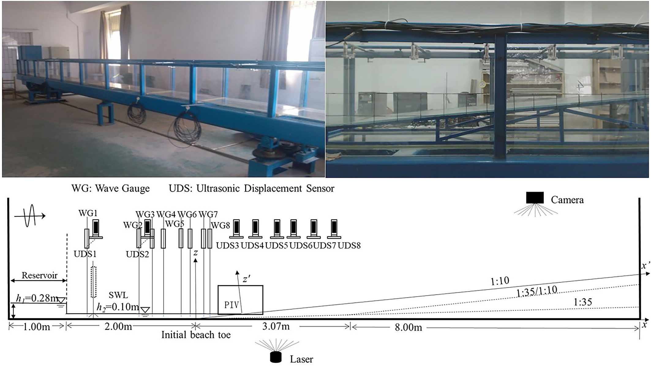
Figure 1 Sketch of the experimental setup and measurement locations.
A three-dimensional Cartesian coordinate system is established in the flume. The initial beach toe is the origin, which is located 2 m from the reservoir gate; the x-axis is located along the center line of the flume bottom with positive value pointing to the bore propagation direction. The y-axis is along the flume width, and the z-axis is vertical with positive value pointing to the opposite direction of the water’s gravity. The time t = 0 s corresponds to an instant of gate opening. In the experiment, the water depth in front of gate h1 was set as 0.28 m, and the water depth behind gate h2 was set as 0.1 m. h1 is the upstream water level, h2 is the downstream water level, and hm is the water depth downstream of the wave head, which can be solved by the shallow water wave theory (Stoker, 1992), as shown in Eq. (1)
U0 is the propagation velocity of the bore. The relationship between hm and U0 can be established through the Froude number, as shown in Eq. (2). The initial water depth is defined as h1/h2, and η0 is defined as hm − h0. When h1 = 0.28 m and h2 = 0.10 m, according to Eq. (2), hm = 0.17 m, U0 = 1.55 m/s, and F0 = 1.56. As indicated in Yeh et al. (1989), when the initial water depth meets h1/h2 > 2.00, a fully developed bore is formed, and when the initial water depth meets h1/h2< 2.00, a wavy bore is formed. In this experiment, the initial depth ratio is 0.28/0.1 = 2.8, and the bores’ developing distance from the gate to the beach toe is 2 m which is about 30η0; thus, fully developed bores can be generated before they reach the beach toes.
2.2 Instrumentation
As also shown in Figure 1, the time series of free surface elevation of this experiment was measured by both WG-50 wave gauges (WG, RBR Ltd., Canada) and ultrasonic displacement sensors (UDS, GE Ltd., Germany). Wave gauges can accurately measure the water level with good linearity based on different capacitances between water and air. These sensors had a response time of 5 ms, the minimum measurement period of WG was 1.5 μs, and the measurement error was 0.4%. Eight gauges (WG1~WG8) were used to measure the waves in the inner surf zone and lower swash zone at selected locations, and the sampling frequency of gauges was set to 50 Hz. However, the intrusive gauges cannot measure the shallower waters; thus, eight non-intrusive sensors (UDS1~UDS8) were arranged in the middle and upper swash zones for the wave measurement. The measurement accuracy of UDS can reach 0.2 mm, and the maximum sampling frequency of the sensors was 20 Hz.
It is worth mentioning that both WG1 and UDS1 were placed at the same location (i.e., x = −1.70 m) for the measurement validation between each other. For different beaches, wave measurements were placed at different cross-shore locations (Table 1).
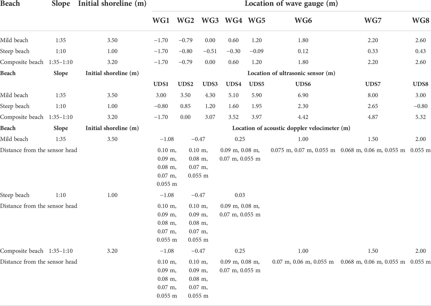
Table 1 Locations of wave gauge, ultrasonic sensor and acoustic doppler velocimeter along the x-axis.
Velocities were measured using both the acoustic Doppler velocimeter (ADV, Nortek Ltd., Norway) and the particle image velocimetry (PIV, TSI Ltd., USA). ADV can measure the velocity with high precision and high frequency, which can ensure the accuracy of the captured velocity data. The non-intrusive PIV velocity measurement technique can avoid the flow interference by the instrument itself, and its spatial resolution is high. It can also provide visual and qualitative observation of the flow field. ADV is used for velocity measurement in the inner surf zone and the lower swash zone. Its specific location is shown in Table 1. In the y dimension, the position of ADV was at the center line of the flume (y = 0 m). In this experiment, the sampling frequency was 100 Hz for the ADV, and the sampling volume height was 9.1 mm. Velocity time series from an ADV tend to become noisy in highly turbulent or aerated flows. At such times, we use winADV for noise processing. When the measured signal-to-noise ratio was higher than 15 or the signal amplitude exceeded 75, this part of the data was discarded and recalculated using the triple difference algorithm.
In the middle and upper swash zones, swash velocities were measured using 16 cross-correlation PIVs on the beach. The camera was computer-controlled to acquire 80 consecutive image pairs (160 images) at 14.5 Hz. It could basically record the flow movement process of a single swash cycle. The image size did not vary from the offshore location to the onshore location with 21 × 21 cm2 size in the field of view (FOV). Laser illumination of the flow for the PIV measurement was a New Wave Solo III double-pulsed, frequency-doubled Nd YAG laser, with 50~120 mJ energy range and 100 Hz sampling frequency. The reflected laser light from the seeding particles was captured by a PowerView 4M Plus high-speed image acquisition, which has 2,048 * 2,048 pixels, 17 Hz sampling frequency, and 1 μs minimum cross-frame time. The software controlling the PIV system timing, image acquisition, and image analysis was Insight 3G. PIV was employed for velocity measurement both in the middle and upper swash zones. The specific location is shown in Table 2.

Table 2 PIV cross-shore position.
In addition, two Logitech C910 HD cameras were used to record the swash zone process, and the resolution of the camera was 1,920 × 1,080. One camera was arranged on top of the flume to record the maximum climbing position of the bore, and the other was set on the side of the flume to monitor the processes of bore collapse, uprush, and backwash.
2.3 Measurement and its validation
Take the steep beach for example, four snapshots of the measured flow patterns over the beach are shown in Figure 2. The time of each snapshot is t = 1.3, 2.0, 2.3, and 7.5 s corresponding to the phases of bore forming, collapse, uprush, and backwash, respectively. After the dam-break wave arrived at the toe of the beach, a fully developed bore was formed, which entrained a significant amount of air, and then the bore collapsed at the shoreline, resulting in further shoreward movement (i.e., uprush). A few seconds later, the flow retreated and its direction turned to the seaward movement (i.e., backwash). The backwash encountered the tail waves. Most importantly, Figure 2D shows that a hydraulic jump formed in the lower swash zone when the bore moved backward. The backwash flow would further move to the left gate and then reflected to start a new swash event. This phenomenon could also be explained by the cross-tank water oscillations (O’Donoghue et al., 2010), which can be taken as swash–swash interactions. The water level oscillations and swash–swash interactions are very important hydrodynamic phenomena in the inner surf and swash zone, which could result in high suspended sediment concentrations and rapid beach evolution (Alsina and Cáceres, 2011). Therefore, the time of water elevation acquisition was set as 2 min, although the time of the single swash cycle was very short as mentioned above.
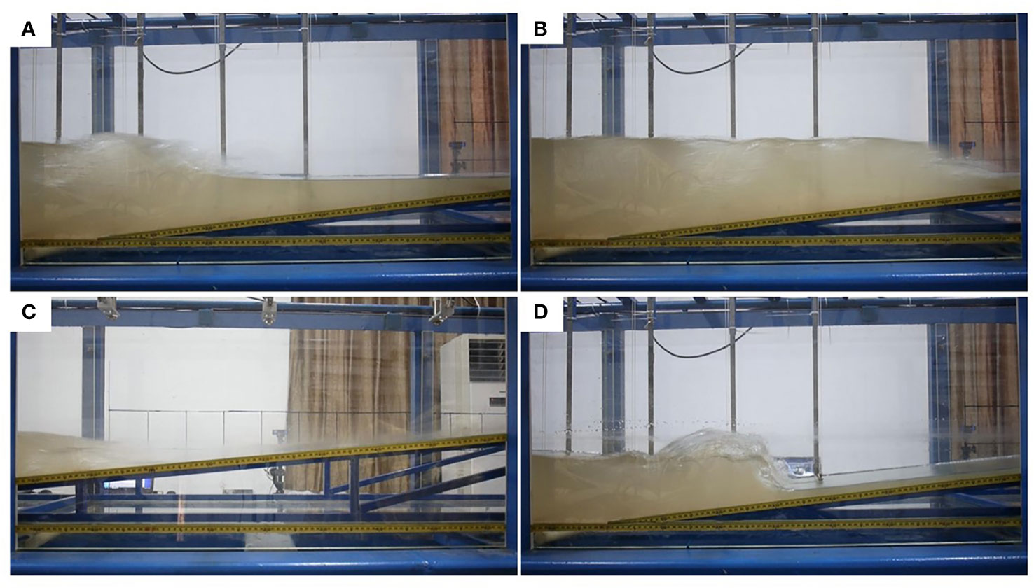
Figure 2 Snapshots of the bore evolution on the steep beach: (A) bore forming, t = 1.3 s; (B) bore collapse, t = 2.0 s; (C) uprush, t = 2.3 s; (D) backwash, t = 7.5 s.
The time series of water surface elevation at each location are measured for 45 repeated runs of the same swash event. The ensemble-averaged depth at locations x and time t is obtained as
where hn(x, t) denotes the measured water depth from the n-th run, with N = 45 in this study. The variance of the measured water depth value is calculated by
Figure 3 shows the statistical values of and at x = −1.70 m, where hsd is the standard deviation of h, . It can be seen from the figure that hsd is generally less than 5% of the water depth. It shows that water surface elevation is highly repeatable among successive experimental runs, indicating that the test repeatability is good. The swash cycle associated with the three beaches varies, and the time of the cycle is 17.5, 7.6, and 11.8 s for the mild beach, steep beach, and composite beach, respectively.
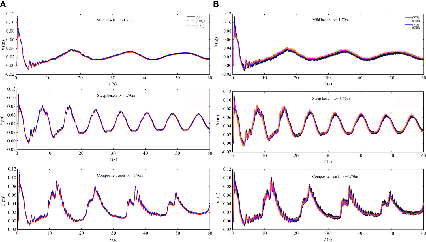
Figure 3 (A) Ensemble-averaged depth time-series and comparison at x = −1.70 m on the three beaches; (B) the comparison of ensemble-averaged depth time series between both WG and UDS at x = −1.70 m on the three beaches.
2.4 Variables obtained from measurements
The cross-shore ensemble-averaged velocity profiles along the water depth are obtained based on the PIV flow measurements
and the variance of is
In Eq. (5), u (x, z, t) represents the instantaneous velocity measured during the nth swash event, and N = 6.
The depth-averaged cross-shore velocity, is obtained from the ensemble-averaged velocity profile as
3 Results
3.1 Visualization of the swash evolution
Snapshots of the measured flow motions are shown in Figure 4 for the three beaches, respectively, based on the PIV images. The instants of the snapshot correspond to four stages, namely, bore formation, collapse, uprush, and backwash, respectively. For all beaches, after the dam-break wave arrives at the toe of the beach, a fully developed bore is formed, which entrains a significant amount of air. The bore travels shoreward on the beach and then collapses at the shoreline, resulting in further uprush of the water. After that, the flow direction reverses to seaward, and the water retreats as the backwash. When comparing among the three beaches, it could be observed that the bore propagating on the steep beach (Figure 4B) results in stronger splashing water, air entrainment, and turbulence flow than those on the mild beach (Figure 4A). This is consistent with the results of O’Donoghue et al. (2010) and Dai et al. (2017) who carried out the experiments on a 1:10 beach. Moreover, the backwash encounters tail wave violently; therefore, the hydraulic jumps could be only observed on both steep and composite beaches (Figures 4B, C).
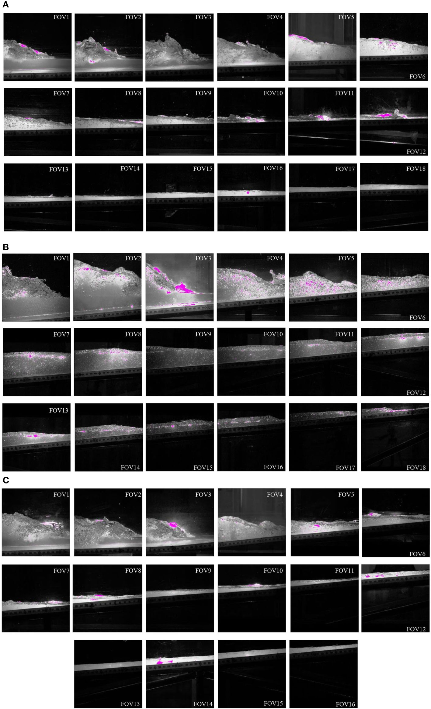
Figure 4 The bore evolution in the selected PIV windows (FOV): (A) mild beach; (B) steep beach; (C) composite beach.
3.2 Shoreline movement
Figure 5 shows the shoreline trajectory (measured by camera video recording) of a single swash cycle for the three tested beaches. In this figure, Rx is defined as the horizontal wave runup distance from the location where still water level meets the beach (initial shoreline, Rx =0) to the location where the swash depth is reduced to 5 mm.
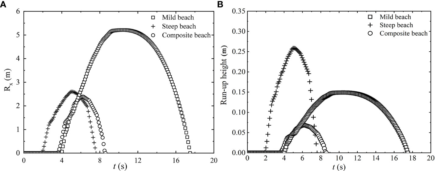
Figure 5 Time series of the shoreline location (Rx) (A) and runup height (B) based on the camera video recording.
For the three beaches, the variations of the shoreline position present different characteristics. The shoreline rises rapidly at the initial stage of uprush, then its increase slows down until it reaches the maximum runup location. At the initial stage of backwash, the shoreline drops relatively slowly, and then its decrease gradually accelerates until it reaches the initial shoreline location (Rx = 0). The bore arrives at the initial shoreline location at t = 4, 2, and 3.6 s following the gate release for the three beaches, respectively, and the initial moving speeds of the shorelines on these beaches are 1.80, 1.60, and 2.00 m/s, respectively. The slope also affects the peak value of Rx and runup height associated with the maximum bore runup: for the mild beach, peak Rx = 5.20 m and runup height was 0.148 m at t = 10 s; for the steep beach, peak Rx = 2.60 m and runup height was 0.258 m at t = 5 s; and for the composite beach, peak Rx = 2.40 m and runup height was 0.068 m at t = 6.3 s. Meanwhile, the durations of uprush and backwash phases for the three beaches are different. The ratio of backwash duration to uprush duration is defined as Rbu. For the mild beach, Rbu = 1.25; for the steep beach, Rbu = 0.84; and for the composite beach, Rbu = 0.70. Thus, the asymmetry between runup and runback phases in the swash zone is larger for the mild slope. The shoreline change of the composite beach has the combined feature of the other two beaches. Because the lower part of the composite slope is gentle, its initial increase of Rx is similar to that on the mild slope. After that, the uprush flow travels to the steep beach part, and the shoreline runup motion takes a shorter time. Thus, Rx is minimum among the three beaches.
3.3 Swash depth
3.3.1 Temporal evolution of the swash depth across the beach
Figure 6 presents the time series of the measured water depth within a single swash cycle for the three beaches. All records are reconstructed from the ensemble-averaged depth at eight sampling locations (measured by WG or UDS) between the toe of the beach and the upper swash zone.
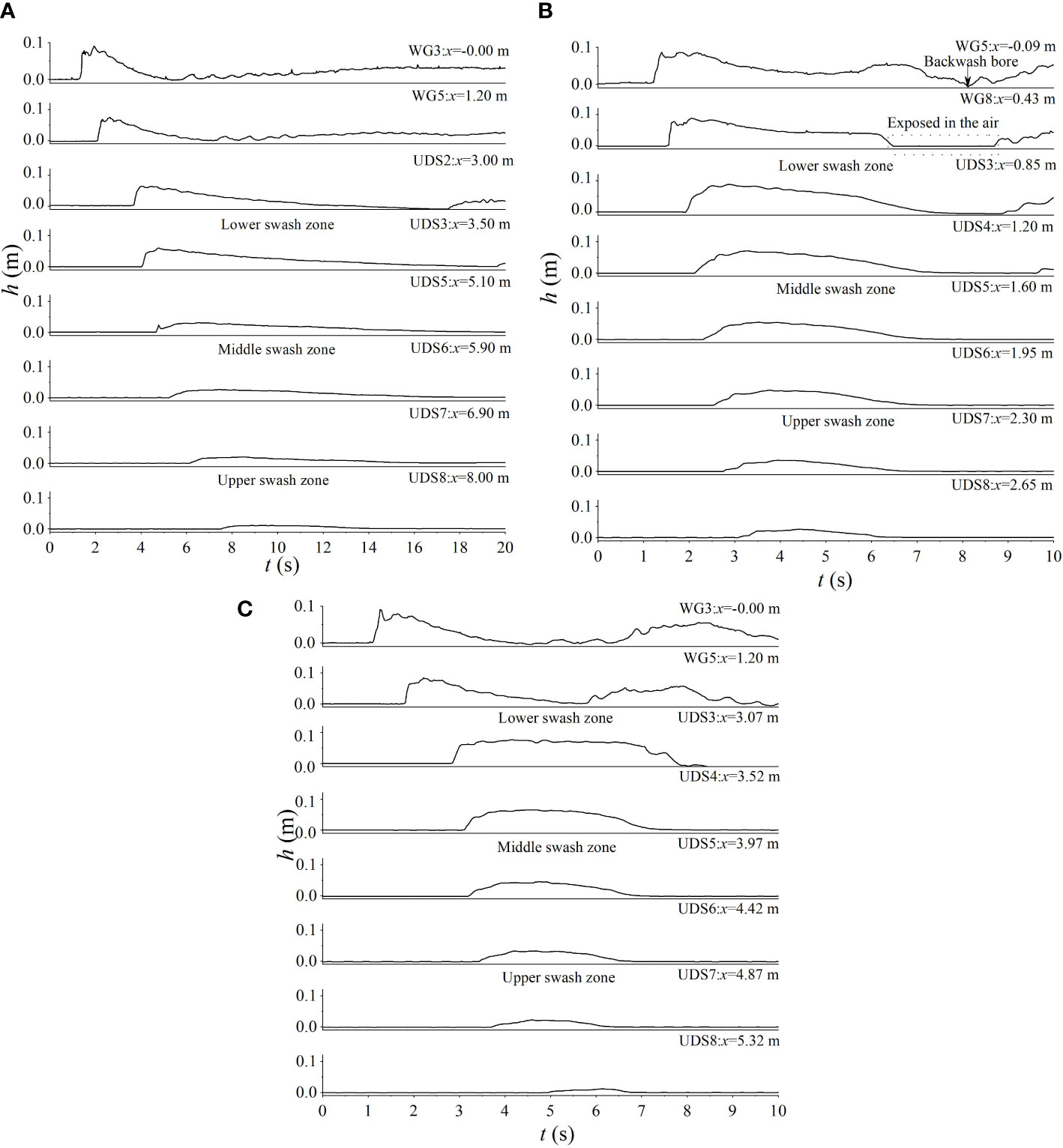
Figure 6 Time series of the measured water depth (h) at eight sampling locations (WG or USD) and comparison of swash depths in different cross-shore sections of the swash zone: (A) mild beach; (B) steep beach; (C) composite beach.
For the mild beach (Figure 6A), the bore arrives at the initial shoreline at 4.0 s with a height of 6.00 cm at DUS2 (x = 3.00 m). When the bore arrives, peak water depth appears and then the depth declines gradually. The whole cycle completes within 17.5 s. Meanwhile, many undulating tail waves appear behind the bore, which are caused by the plunging breaking waves (Kikkert et al., 2012). These periodic fluctuations are largest at the lower swash zone but disappear as they move further shoreward. Note that there is no hydraulic jump occurring on the mild slope.
Compared to that on the mild beach, the bore arrives at the initial shoreline at 1.25 s with a height of 8.60 cm at WG5 (x = −0.09 m) on the steep beach (Figure 6B). It then reaches the initial shoreline by 2.0 s with a height of 7.20 cm at UDS3. In the late stage of uprush, the water depths in the lower (e.g., x = 0.85 m) and middle (e.g., x = 1.60 m) swash zone begin to decrease at the transitional instant when flow direction reverses from uprush to backwash. The backwash flow is formed at WG5. After the water retreats, a series of very turbulent localized rundown hydraulic jumps are generated as discussed in Section 3.1. These hydraulic jumps are considered to be a very important forcing to suspend the sediments. However, because the water layer is very thin, the capacitance wave gauge (WG8) is exposed t the air and could not obtain any effective data for the hydraulic jumps. A single swash cycle on this beach is about 7.6 s.
For the composite beach, the bore arrives at the initial shoreline at 3.6 s with a height of 7.40 cm at UDS3 (x = 3.07 m), which is closer to the mild slope in that the lower section of the slope is identical to the mild beach (1:35). After the bore travels on its upper section with the steep slope of 1:10, the bore is found to be dissipated faster (UDS4, x = 3.52 m). During the later uprush and the backwash stages, the bore moves in a similar way to that on the steep beach. Hydraulic jumps could not be clearly observed on this beach. The swash cycle is about 11.8 s, which is in between the other two beaches.
In general, the variation characteristics of swash depth at these sampling locations are similar to those reported in field observations (e.g., Hughes et al., 1997; Masselink and Hughes, 1998; Hughes and Baldock, 2004) and in laboratory experiments (Cowen et al., 2003; Barnes et al., 2009; O’Donoghue et al., 2010; Kikkert et al., 2012; Chen et al., 2016).
3.3.2 Comparison of the swash depths in different sections of the swash zone
In Figure 6, three different cross-shore locations are selected to represent the lower, middle, and upper swash zones.
Overall, in the lower swash zone, the water depth of the swash in the uprush phase rapidly increases to the maximum (5.70~8.30 cm) and gradually decreases after a period of fluctuation, but the flow does not reverse at this time. In the middle swash zone, before the swash depth reaches the maximum (2.50~5.30 cm), the swash depth decreases slowly. After the flow reversal, the depth decreases rapidly. In the upper swash zone, the swash depth decreases rapidly after reaching the maximum water depth (1.00 ~3.60 cm), and there is no fluctuation in the swash depth on this zone compared to the lower and middle swash zones.
The beach slope affects the maximum value of swash depth as well as the asymmetry of its temporal variation. The maximum swash depth on the mild slope is 5.80 cm (x = 3.50 m), while on the steep slope, it is 8.40 cm (x = 0.85). In addition, a distinctive feature of the mild beach is that swash depth in all sections of the swash zone rapidly increases to the peak after the bore arrives, and then it gradually decreases without fluctuation. Thus, the asymmetry in the temporal variation of swash depth is relatively large during this swash cycle. However, on steep and composite slopes, the drop of water depth fluctuates.
3.4 Swash velocity
3.4.1 Cross-shore velocity profiles along the water depth in different sections of the swash zone
Figure 7 depicts in the PIV measuring windows. Three different cross-shore locations (for the mild beach: x = 3.75, 4.20, and 5.50 m; for the steep beach: x = 0.90, 1.90, and 2.90 m; for the composite beach: x = 3.25, 4.25, and 4.70 m) are selected to represent the lower, middle, and upper swash zones. The profiles of are irregular in the lower swash zone where the bore is collapsing on the beach because the bore generates turbulence with significant air entrainment. After that, the profiles develop into a typical “forward-leaning” shape during the uprush phase, and they become almost depth-uniform in the later stage of the uprush and the initial stage of the backwash. Eventually, they gradually evolve into a non-uniform pattern as the velocity increases and depth decreases in the last stage of backwash. The maximum values of reach up to 1.5~1.7 m/s for the three beaches after the bore arrival.
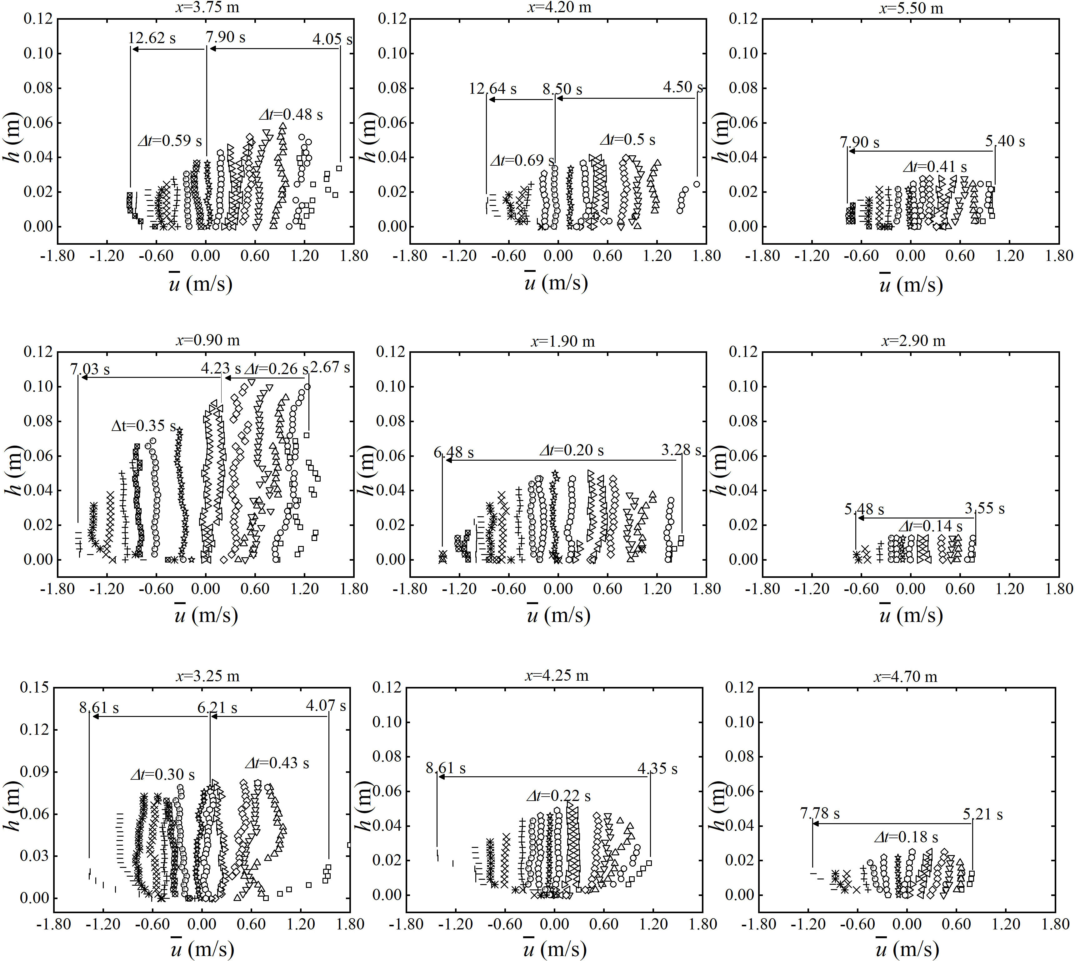
Figure 7 Temporal evolution of the ensemble-averaged, cross-shore velocity profiles at different cross-shore positions for the three beaches. Upper row: mild beach; middle row: steep beach; lower row: composite beach. In this figure, symbols of the same type represent the same profile, and the time interval between two successive profiles is Δt. Arrows indicate the evolution of profiles in time.
For all beaches, the change of is the highest near the bed, and approaches near depth-uniform when the depth value is greater than 0.02 m. During the uprush phase, the flow depth increases sharply, and the flow velocity decreases until it goes to zero as the uprush reaches the maximum runup. During the backwash phase, the flow depth decreases rapidly, and the flow velocity increases until it reaches the peak backwash velocity. This leads to a very steep near-bed gradient in the cross-shore velocity profiles. For example, at the instant of maximum backwash velocity at x = 0.9 m on the steep beach, the velocity increases from zero at the bed to −1.5 m/s within a depth of 1 cm.
Comparing the velocity profiles among the three beaches indicates that the gentler the slope is, the larger the degree of asymmetry in the maximum velocity between the uprush and backwash phases. For the mild beach at x = 3.25 m, the velocity reaches 1.70 m/s after bore arrival and −0.60 m/s during the later stage of the backwash. The velocity changes more rapidly for the steep beach and the composite beach than that for the mild beach which is due to the relatively shorter duration of backwash on steep and composite beaches compared to that on the mild beach. During the transition period, the bottom flow reverses earlier than at the top of the column. Three-dimensional CFD solvers, such as those based on RANS equations (Zhang and Liu, 2008; Torres-Freyermuth et al., 2013; Pintado-Patiño et al., 2015; Kim et al., 2017), have shown this kind of phenomenon.
3.4.2 Depth-averaged cross-shore velocity profiles in different sections of the swash zone
Time-series depth-averaged velocity for the lower, middle, and upper swash zones of the three beaches are presented in Figure 8.
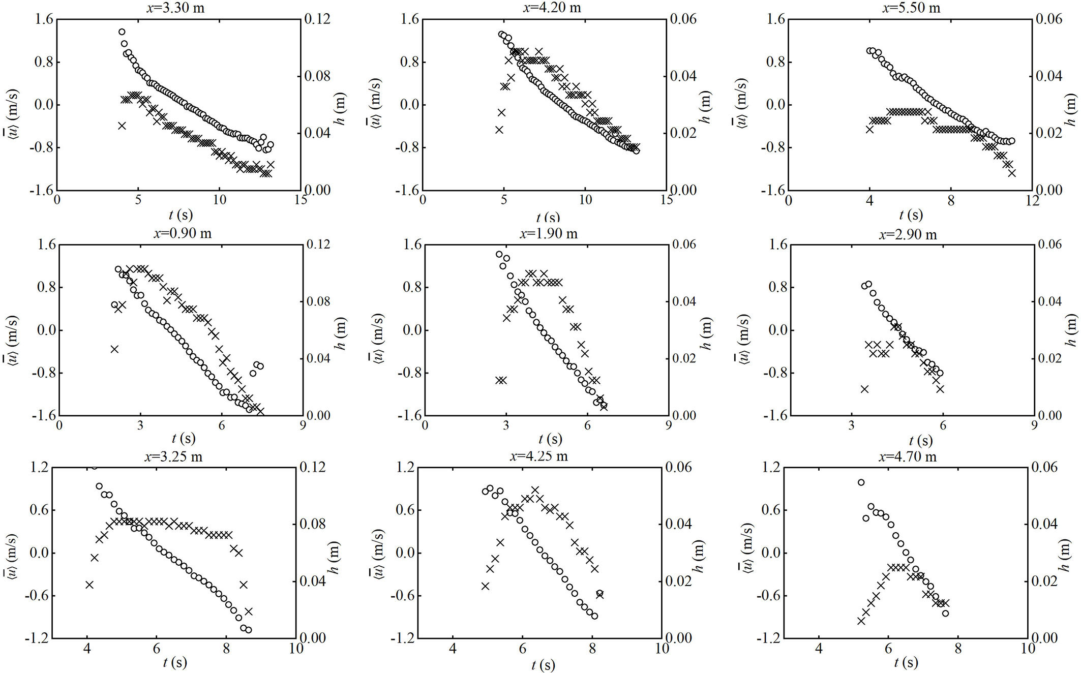
Figure 8 Time series of depth-averaged streamwise velocity (circle) and water depth (cross) for selected cross-shore locations. Upper row: mild beach; middle row: steep beach; lower row: composite beach.
Due to the air bubble’s influence, the swash depth is not smooth, causing difficulty in determining velocity near the water surface. In the experiments, the velocity near the interface between air and water is hard to measure. If there is an abnormal coefficient of variation (), the velocity vectors will be discarded. On the three beaches, the uprush flow velocity, , reaches the maximum at the time of bore arrival, which falls into the range of 1.2~1.6 m/s. After that, it gradually declines in the uprush stage. During the backwash stage, the reverse flow gradually rises to the maximum due to the combined effect of bed friction and gravity, which is about −0.9~−1.6 m/s. Maximum uprush velocity is comparable to the maximum backwash velocity for both the steep beach and the composite beach, whereas the maximum uprush velocity (about 1.5 m/s) is higher than the maximum backwash velocity (about −0.8 m/s) for the mild beach. Therefore, the asymmetry in the depth-averaged velocity is more significant for the mild beach than the other two. In general, variations of the present depth-averaged velocity match well with those experimental observations (e.g., Masselink and Hughes, 1998; Puleo et al., 2000; Hughes and Baldock, 2004) and laboratory measurements (e.g., O’Donoghue et al., 2010; Kikkert et al., 2012) in the literature. In addition, Figure 8 also shows the swash depth variation at the same location. In the lower swash zone, a peak positive velocity and a peak water depth are achieved simultaneously at the position close to the initial shoreline. The maximum uprush velocity in the middle swash zone appears to be higher than that in the upper swash zone. The main discrepancies occur at the middle and upper swash zones, the time to reach the maximum uprush velocity is earlier than the time to reach the maximum depth of swash, and this phenomenon is more evident in the upper swash zone.
As discussed above, the velocity profile is not always depth-uniform. One reason is that the velocity of the uprush is relatively high at the initial stage, and the other reason is that the backwash depth is very thin at the late stage of the backwash. A parameter (β) to evaluate the degree of depth uniformity is introduced by O’Donoghue et al. (2010), and it is the deviation of the profile from its depth-averaged value
where β = 0 implies the perfect depth uniformity and an increasing β implies an increasing depth non-uniformity. β plotted against for the lower, middle, and upper swash zones of the three beaches is presented in Figure 9. At the instants close to the bore arrival and the end of the backwash, the depth-averaged velocity reaches the maximum uprush and backwash velocities, respectively. The distribution of β is near symmetrical around in each section on the three beaches, indicating that there is no significant difference in velocity distribution between uprush flow and backwash flow, which is also obtained by O’Donoghue et al. (2010). Because of the strong turbulence that exists in the initial stage of the uprush flow, and there is a high-speed thin sheet flow in the later stage of the backwash, the value of β in each zone is large, indicating that the distribution of velocity along the water depth is strongly non-uniform. This feature is the most dominant for the composite beach, while for beaches with a single slope, β is almost less than 0.20 m/s.
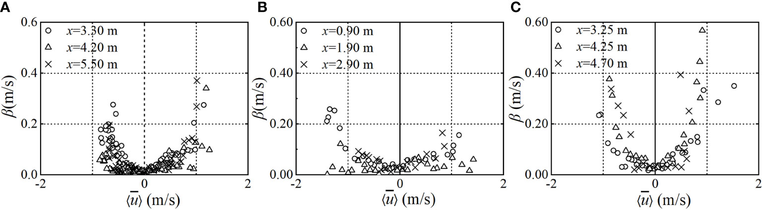
Figure 9 A parameter (β) to evaluate the degree of depth uniformity of the cross-shore velocity profile: (A) mild beach; (B) steep beach; (C) composite beach.
3.5 Vortex structure
3.5.1 Classification of the vortex structures
In the literature, Gilb (2005) defined five special vortex structures. The spinning vortex (SPV) is spinning around a center pivot point. Previous studies have shown that its formation is closely related to the turbulence of the surrounding flow, and it is the most common vortex structure. The feature of the outward propagating spiral vortex (OPSV) is that the velocity vectors rotate and propagate out from the rotation center. The main reason for its formation is that the water above is mixed into the measuring area and tends to diffuse around. The shape of the OPSV is similar to that of the SPV, but the OPSV often shows unstable characteristics. Gilb (2005) pointed out that the OPSV is the initial shape of vortex formation and will gradually develop into the SPV with the movement and diffusion of the vortex. In the flow phenomenon of water moving spirally from the periphery to the rotation center, this vortex is called inward propagating spiral vortex (IPSV). In the existing studies, IPSV is difficult to capture and has no temporal and spatial correlations with SPV and OPSV. Its formation is mainly due to the notable change of pressure distribution in the water body caused by the downburst structure generated in the flow movement as will be discussed later, and the surrounding water accumulates in the low-pressure area. Under the action of seabed friction, two masses of fluids flowing in opposite directions produce a strong shear effect, and a circumferential flow is formed in the local areas. This vortex structure is called the shear vortex (SV). In addition, the last type is the downburst structure, which is caused by the jet impinging on the bed surface, resulting in a diffusion of the surrounding water.
3.5.2 Temporal and spatial characteristics of the vortex structure
In Table 3, the vortex structure characteristics at different PIV windows in the experiments are presented using the PIV-measured flow field. It can be found that vortex structures such as the SPV, OPSV, and downburst structure can be captured. Subsequently, the spatial and temporal characteristics of the vortex structures, including both spatial and temporal correlations, are analyzed.
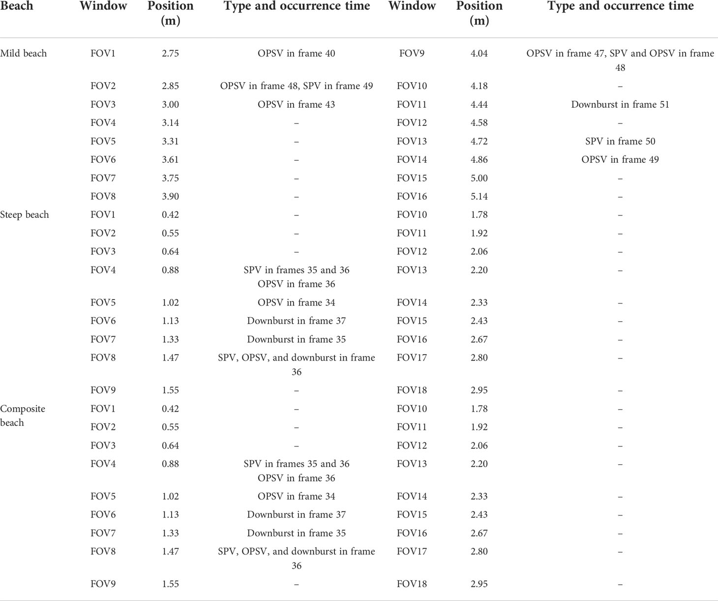
Table 3 The characteristics of the vortex structure.
Spatial correlation focuses on different types of vortex structure mainly appearing in the window near the initial shoreline. Table 3 shows that the fewer PIV windows can capture vortex structures on the steep beach than that on the mild and composite beaches. Because the energy dissipation of runup flow is significant under steep beach condition, the flow velocity decreases rapidly to zero in a short time, and the number of windows included in the transition period is significantly reduced; therefore, the extent of the vortex structure is reduced. At the same time, it is found that the location of slope change has a great influence on the flow of the composite beach. Local water disturbance is formed near the beach, and eventually, a small-scale unstable OPSV vortex is formed (Figure 10). Frames 41~45 can capture the physical movement of disturbed water climbing near the bed surface. With decreased impact in the process of bore runup, the surrounding flow decreases significantly, and the range of moving water near the bed is enlarged gradually. At frame 46, an obvious OPSV is formed.
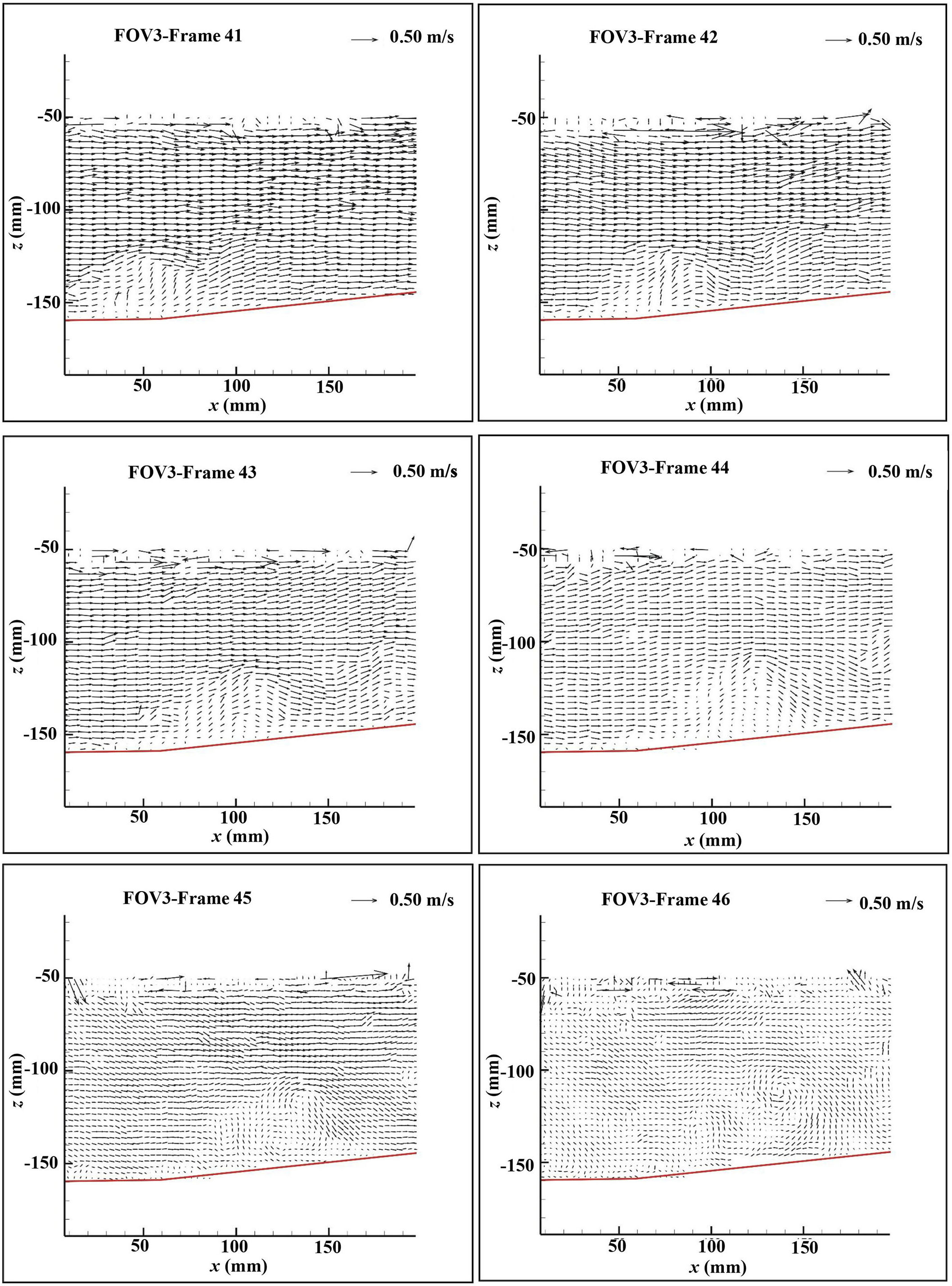
Figure 10 Formation of vortex structures at the location of beach slope transition on the composite beach.
Temporal correlation focuses on the vortex structures formed during the transition period. At this stage, due to the gradual reduction of the momentum in uprush flow, the velocity at different depths decreases, leading to the intensification of the disturbance, the formation of different velocity zones, and then the increase of the pressure gradient between adjacent water layers. At the same time, under the combined action of gravity and bed friction, the flow direction in some areas changes significantly, with a strong mixing of vortices and violent swash motions. The above mechanisms lead to the formation of SPV and OPSV as shown in Figures 11A, B. During the previous experiments, some scholars (Basco, 1985; Gilb, 2005) found two downburst structures with different scales, and the structural size is 0.34 × 0.33 m, but only small-scale downburst structures are captured at the transition stage of this experiment. As shown in Figure 11C, the downburst structure size is 0.09 × 0.09 m and only occupies 18% of the PIV window.
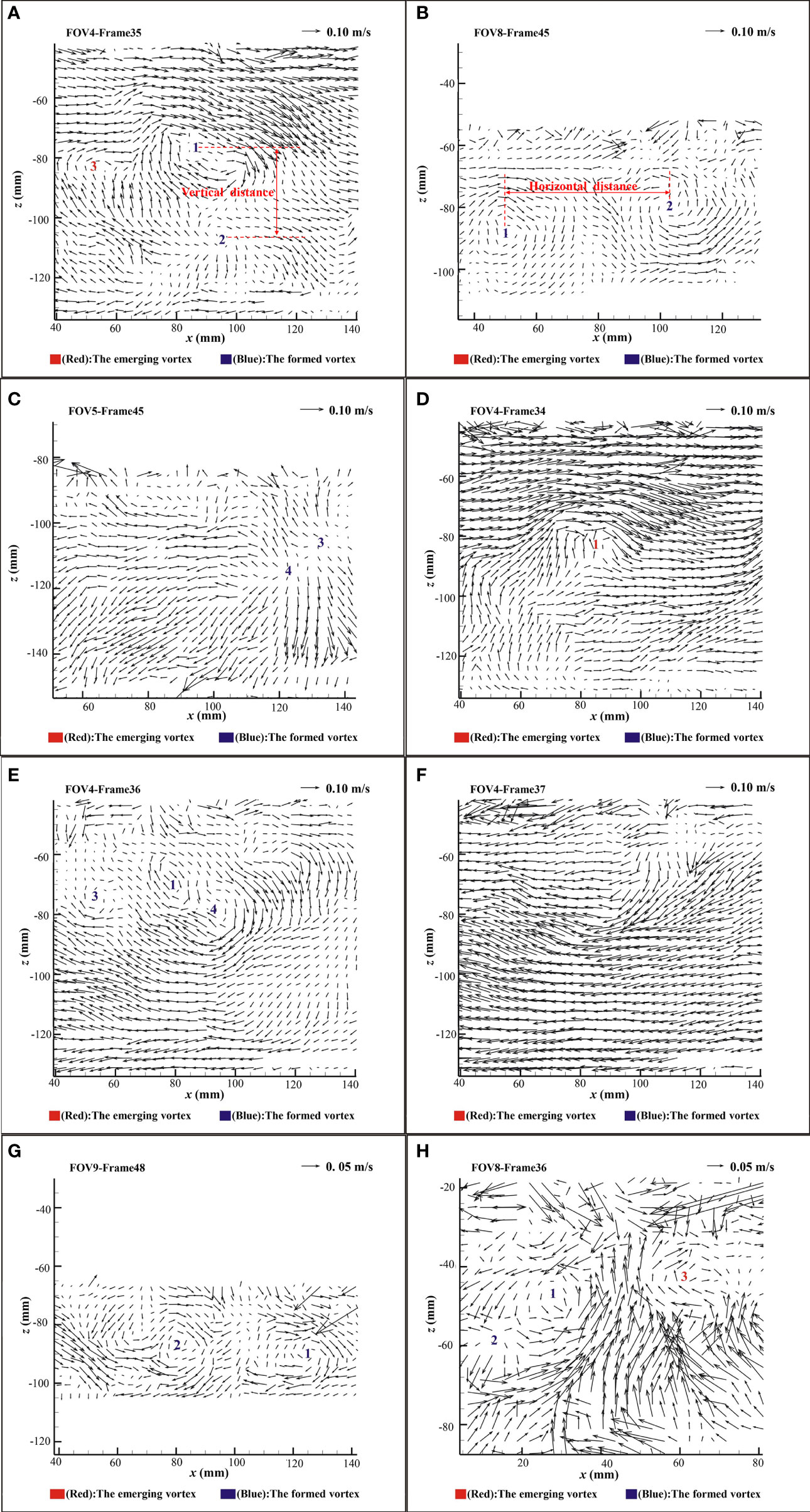
Figure 11 Vortex structures at different PIV windows. (A) SPV (indicated by “1”) and OPSV (indicated by “2”) on the steep beach. (B) SPV and OPSV on the composite beach. (C) Downburst structure on the composite beach. (D–F) Formation and evolution of vortices in FOV4 (steep beach). (G) A different vortex structure coexists in a frame on the mild beach. (H) A different vortex structure coexists in a frame on the steep beach.
3.5.3 Coherent structure
Turbulent motion is not completely irregular. There is possibly a certain coherent structure, that is, a detectable regular motion is formed in the seemingly irregular flow. This regular motion is important to the fluctuating characteristics of turbulence. Taking the mild beach as an example, Figure 11 shows the process of vortex formation and evolution in the typical PIV window FOV4 and FOV8 on the steep beach, respectively. With the rapid reduction of the runup flow impact, the flow rate near the beach changes notably under the combined effect of gravity, friction, and other factors. The upwelling phenomenon occurs near the beach, and the upwelling is mixed with the mainstream, which promotes the disturbance of local flow. This kind of flow mixing is the key factor leading to the formation of the vortex structure. Frames 34 and 35 capture the complete formation process of the SPV, and frames 35 and 36 capture that of the OPSV. During the transition period, there are many vortex structures with different scales in the flow. These vortices form a complex vertical vortex structure system, which enhances the turbulence of flow in the swash zone as shown in frame 35. From frame 35 to frame 36 in Figures 11A, E, because of the impact of high-speed flow, SPV splits into SPV and OPSV, and OPSV disappears. Similar phenomena are also captured in other windows, and SPV and OPSV coexist also in frame 48 of Figure 11G and frame 45 of Figure 11B. SPV and downburst structure coexist in frame 36 of Figure 11H. The flow in the swash zone is highly intermittent, which leads to the transformation, division, aggregation, and disappearance of vortices during the process of vortex movement.
3.5.4 Scale analysis of the vortex structure
According to the analysis in the previous section, there may be two or more vortices within the PIV window. In order to study the relationship between vortex structures, Gilb (2005) introduced the concepts of transverse distance and vertical distance between vortices. The transverse distance between adjacent vortices represents the projection length of the distance between vortex centers in the x-axis direction (see Figure 11B), and the vertical distance represents the projection length of the distance between vortex centers in the z-axis direction (see Figure 11A). Table 4 shows the scale of the vortex structure. It is found that the transverse distance between adjacent vortices on mild beach ranges from 3.7 to 7.00 cm and the vertical distance ranges from 0.20 to 0.60 cm. The transverse distance between adjacent vortices on steep beach ranges from 0.40 to ~5.70 cm, and the vertical distance ranges from 0.40 to ~3.10 cm. The transverse distance between adjacent vortices of composite beach ranges from 0.30 to 5.20 cm, and the vertical distance ranges from 0.70 to 1.00 cm. Meanwhile, frame 35 and frame 36 of Figure 11 also show that the distance between the large-scale vortices is significantly smaller than that of the small-scale vortices. However, since many vortices are generated in the experiments, a specific relationship between the scale of the vortices and the distance between the vortices is unable to be identified at the moment, and further study is required.

Table 4 Scale of the vortex structure.
4 Conclusions
This experimental study aims to investigate the detailed hydrodynamics of dam-break bore-driven swash on impermeable smooth beaches in a flume. A mild slope, a steep slope, and a composite slope are tested, respectively. Experimental measurements of wave level and flow are obtained via combined advanced measuring techniques based on the WG, UDS, ADV, and PIV, which can help to analyze the hydrodynamic characteristics of the swash more comprehensively. Based on the experimental results, hydrodynamic characteristics such as shoreline movement, swash depth, swash velocity, and vortex structure in the swash zone are analyzed in detail. The main conclusions drawn from this study are listed as follows:
After the bore collapses, the bore is involved in a large number of air bubbles. A high-speed thin sheet flow is generated during the uprush and backwash stages. In the late backwash stage, hydraulic jumps can be found on the steep beach. Comparing the swash processes among the three beaches shows that the bore propagating on the steep beach results in stronger splashing, air entrainment, and turbulence flow than on the mild beach.
The analysis of shoreline motion shows that the shoreline rises rapidly at the initial stage of uprush, then its increase slows down until it reaches the maximum runup location. At the initial stage of backwash, the shoreline drops relatively slowly, and then its decrease gradually accelerates until it reaches the initial shoreline location. However, there are differences in the time when the bore arrives at the initial shoreline location, the initial velocity of the bore, and the peak horizontal wave runup distance on the three beaches. The main performance is that the initial moving speed of the shorelines was maximum on the steep beach, and on the composite beach, velocity was minimum. On the mild beach, the horizontal wave runup distance (Rx) was maximum.
Beach slope affects the time the swash reaches the initial shoreline and the single swash cycle. The time for the swash to reach the initial shoreline is the shortest on the steep beach and the longest on the mild beach. The swash cycle is the shortest on the steep beach and the longest on the mild beach. Moreover, for the composite beach, the time for the swash to reach the initial are between the steep beach and the mild beach.
For all three beaches, the flow depth rapidly increases to the maximum depth after bore arrival. Then, maximum depth is followed by a period of slowly decreasing depth. The bore continues to run up the slope and the depth decays rapidly immediately. The rate of decreasing depth increases during the backwash until the late stage in the backwash when the depths have become small. Furthermore, for different locations of the swash zone, the wash depth shows different trends: before the swash reverses, the water surface fluctuates in the low swash zone, but that is not apparent in the middle swash zone and there is no fluctuation in the upper swash zone.
In the uprush phase and the early backwash phase, the ensemble-average velocity is close to the uniform distribution of water depth, but in the middle and late backwash phases, the ensemble-average velocity distribution is not uniform. In addition, the features of depth-averaged velocity show that the maximum uprush velocity is greater than the maximum backwash velocity on the mild beach, but there is little difference between the steep beach and the composite slope. The asymmetry of swash duration and the maximum velocity during the uprush and backwash phases are more significant on the mild beach.
The vortex structures such as the SPV, OPSV, and downburst are captured in the experiments on the three beaches. Vortex structures are formed during the transition period on the three beaches, and different types of vortex structures mainly appear near the initial shoreline. On the steep beach, the fewer PIV windows can capture vortex structures than those on the mild and composite beaches. There are coherent structures in the turbulence, especially in the transition period. The phenomena of transformation, division, aggregation, and disappearance of vortices during the process of vortex movement can also be observed. Furthermore, there are different ranges of the horizontal and vertical transverse distances between adjacent vortices on the three beaches.
The detailed experimental data analyses in this study not only help to better interpret the physical process of bore-driven swash on the beach but also provide the data reference for further numerical modeling investigations. However, there is a scaling effect in experimental research, and the present study focuses only on the immobile bed without sediment movement. Further research will be directed to the sediment transport in the swash zone and the response of bed morphological change to the action of the swash.
Data availability statement
The raw data supporting the conclusions of this article will be made available by the authors, without undue reservation.
Author contributions
BD and CJ designed the experimental methods presented in this manuscript and coordinated the laboratory research. BD and YY collected the laboratory measurements. BD and WZ worked on data analysis. WZ wrote the original manuscript draft. BD, CJ, and YY participated in the manuscript preparation and improvement. All authors contributed to the article and approved the submitted version.
Funding
This study was supported financially by the National Natural Science Foundation of China (Grant numbers 51979015, 51839002) and the National Key Research and Development Program of China (grant number 2021YFB2601100). Partial support was also provided by the Science Foundation of Hunan Province, China (grant number 2021JJ30707), and the Science and Technology Innovation Program of Hunan Province, China (grant number 2020RC3037, 20hnkj019).
Acknowledgments
The first author thanks Dr. Zhiyuan Wu at Changsha University of Science and Technology, China, for the assistance in the laboratory work.
Conflict of interest
The authors declare that the research was conducted in the absence of any commercial or financial relationships that could be construed as a potential conflict of interest.
Publisher’s note
All claims expressed in this article are solely those of the authors and do not necessarily represent those of their affiliated organizations, or those of the publisher, the editors and the reviewers. Any product that may be evaluated in this article, or claim that may be made by its manufacturer, is not guaranteed or endorsed by the publisher.
References
Aagaard T., Hughes M. G. (2006). Sediment suspension and turbulence in the swash zone of dissipative beaches. Mar. Geol. 228 (1–4), 117–135. doi: 10.1016/j.margeo.2006.01.003
Aboulatta W., Dodd N., Briganti R., Kasem T. H. M. A., Zaki M. A. F. (2020). Modelling swash zone hydrodynamics using discontinuous galerkin finite element method. J. Waterw. Port. Coast. 147 (2) , 04040051. doi: 10.1061/(ASCE)WW.1943-5460.0000618
Alsina J. M., Cáceres I. (2011). Sediment suspension events in the inner surf and swash zone. measurements in large-scale and high-energy wave conditions. Coast. Eng. 58 (8), 657–670. doi: 10.1016/j.coastaleng.2011.03.002
Alsina J. M., Falchetti S., Baldock T. E. (2009). Measurements and modelling of the advection of suspended sediment in the swash zone by solitary waves. Coast. Eng. 56, 621–631. doi: 10.1016/j.coastaleng.2009.01.007
Bakhtyar R., Barry D. A., Yeganeh-Bakhtiary A., Ghaheri A. (2009). Numerical simulation of surf–swash zone motions and turbulent flow. Adv. Water. Reso. 32 (2), 250–263. doi: 10.1016/j.advwatres.2008.11.004
Barnes M. P., O’Donoghue T., Alsina J. M., Baldock T. E. (2009). Direct bed shear stress measurements in bore-driven swash. Coast. Eng. 56 (8), 853–867. doi: 10.1016/j.coastaleng.2009.04.004
Basco D. R. (1985). A qualitative description of wave breaking. J. Waterw. Port. Coast. 111 (2), 171–188. doi: 10.1061/(ASCE)0733-950X(1985)111:2(171)
Bergsma E. W., Blenkinsopp C. E., Martins K., Almar R., de Almeida L. P. M. (2019). Bore collapse and wave run-up on a sandy beach. Cont. Shelf. Res. 174, 132–139. doi: 10.1016/j.csr.2019.01.009
Briganti R., Dodd N., Pokrajac D., O’Donoghue T. (2011). Nonlinear shallow water modelling of bore-driven swash: Description of the bottom boundary layer. Coast. Eng. 58 (6), 463–477. doi: 10.1016/j.coastaleng.2011.01.004
Briganti R., Torres-Freyermuth A., Baldock T. E., Brocchini M., Dodd N., Hsu T. J., et al. (2016). Advances in numerical modelling of swash zone dynamics. Coast. Eng. 115, 26–41. doi: 10.1016/j.coastaleng.2016.05.001
Brocchini M., Baldock T. E. (2008). Recent advances in modeling swash zone dynamics: Influence of surf-swash interaction on nearshore hydrodynamics and morphodynamics. Rev. Geophysics. 46 (3), RG3003. doi: 10.1029/2006RG000215
Butt T., Russell P., Puleo J. A., Miles J., Masselink G. (2004). The influence of bore turbulence on sediment transport in the swash and inner surf zones. Cont. Shelf Res. 24(7–8), 757–771. doi: 10.1016/j.csr.2004.02.002
Chardón-Maldonado P., Pintado-Patiño J. C., Puleo J. A. (2016). Advances in swash-zone research: Small-scale hydrodynamic and sediment transport processes. Coast. Eng. 115, 8–25. doi: 10.1016/j.coastaleng.2015.10.008
Chen B. T., Kikkert G. A., Pokrajac D., Dai H. J. (2016). Experimental study of bore-driven swash–swash interactions on an impermeable rough slope. Coast. Eng. 108, 10–24. doi: 10.1016/j.coastaleng.2015.10.010
Cowen E. A., Mei Sou I., Liu P. L. F., Raubenheimer B. (2003). Particle image velocimetry measurements within a laboratory-generated swash zone. J. Eng. Mech. 129 (10), 1119–1129. doi: 10.1061/(ASCE)0733-9399(2003)129:10(1119
Cox D. T., Anderson S. L. (2001). Statistics of intermittent surf zone turbulence and observations of Large eddies using PIV. Coast. Eng. 43 (2), 121–131. doi: 10.1142/S057856340100030X
Cox D. T., Kobayashi N. (2000). Identification of intense, intermittent coherent motions under shoaling and breaking waves. J. Geophysical Res-Oceans 105 (C6), 14223–14236. doi: 10.1029/2000JC900048
Dai H. J., Kikkert G. A., Chen B. T., Pokrajac D. (2017). Entrained air in bore-driven swash on an impermeable rough slope. Coast. Eng. 121, 26–43. doi: 10.1016/j.coastaleng.2016.10.002
Deng B., Jiang C. B., Zhao L. P., Tang H. S. (2012). Three-dimensional numerical study on bore driven swash. Asian Pacific Coasts 2011 2011, 1270–1278. doi: 10.1142/9789814366489_0151
Ebrahimi A., Askar M. B., Pour S. H., Chegini V. (2015). Investigation of various random wave run-up amounts under the influence of different slopes and roughnesses. Env. Cons. J. 16 (se), 301–308. doi: 10.36953/ECJ.2015.SE1635
Gilb J. L. (2005). Experimental study of Large turbulent structures in a breaking solitary wave using particle image velocimetry. [Doctoral dissertation]: South Dakota state university. Brookings, South Dakota
Guard P. A., Baldock T. E. (2007). The influence of seaward boundary conditions on swash zone hydrodynamics. Coast. Eng. 54 (4), 321–331. doi: 10.1016/j.coastaleng.2006.10.004
Hammeken A. M., Simons R. R. (2017). Numerical study on the influence of infiltration on swash hydrodynamics and sediment transport in the swash zone. 35th Int. Conf. Coast. Eng. 3(35), currents.3. doi: 10.9753/icce.v35.currents.3
Hughes M. G., Baldock T. E. (2004). Eulerian flow velocities in the swash zone: Field data and model predictions. J. Geophys. Res-Oceans 109, C08009 . doi: 10.1029/2003JC002213
Hughes M. G., Masselink G., Brander R. W. (1997). Flow velocity and sediment transport in the swash zone of a steep beach. Mar. Geol. 138 (1-2), 91–103. doi: 10.1016/S0025-3227(97)00014-5
Hu P., Xie J., Li W., He Z., Marsooli R., Wu W. (2020). A RANS numerical study of experimental swash flows and its bed shear stress estimation. Appl. Ocean Res. 100, 102145. doi: 10.1016/j.apor.2020.102145
Jaffe B. E., Rubin D. M. (1996). Using nonlinear forecasting to learn the magnitude and phasing of time-varying sediment suspension in the surf zone. J. Geophys Res-Oceans 101 (C6), 14283–14296. doi: 10.1029/96JC00495
Jiang C. B., Deng B., Hu S. X., Tang H. S. (2013). Numerical investigation of swash zone hydrodynamics. Sci.China Technological Sci. 56, 3093–3103. doi: 10.1007/s11431-013-5389-9
Kelly D. M., Dodd N. (2010). Beach-face evolution in the swash zone. J. Fluid Mech. 661 (12), 316–340. doi: 10.1017/S0022112010002983
Kikkert G. A., O’Donoghue T., Pokrajac D., Dodd N. (2012). Experimental study of bore-driven swash hydrodynamics on impermeable rough slopes. Coast. Eng. 60, 149–166. doi: 10.1016/j.coastaleng.2011.09.006
Kikkert G. A., Pokrajac D., O'Donoghue T., Steenhauer K. (2013). Experimental study of bore-driven swash hydrodynamics on permeable rough slopes. Coast. Eng. 79, 42–56. doi: 10.1016/j.coastaleng.2013.04.008
Kim Y., Zhou Z., Hsu T. J., Puleo J. A. (2017). Large Eddy simulation of dam-break-driven swash on a rough-planar beach. J. Geophys Res-Oceans. 122 (2), 1274–1296. doi: 10.1002/2016JC012366
Longo S. (2009). Vorticity and intermittency within the pre-breaking region of spilling breakers. Coast. Eng. 56 (3), 285–296. doi: 10.1016/j.coastaleng.2008.09.003
Masselink G., Hughes M. (1998). Field investigation of sediment transport in the swash zone. Cont. Shelf Res. 18 (10), 1179–1199. doi: 10.1016/S0278-4343(98)00027-2
Masselink G., Russell P. (2006). Flow velocities, sediment transport and morphological change in the swash zone of two contrasting beaches. Mar. Geol 227 (3-4), 227–240. doi: 10.1016/j.margeo.2005.11.005
Masselink G., Russell P., Turner I., Blenkinsopp C. (2009). Net sediment transport and morphological change in the swash zone of a high-energy sandy beach from swash event to tidal cycle time scales. Mar. Geol. 267 (1-2), 18–35. doi: 10.1016/j.margeo.2009.09.003
Miles J., Butt T., Russell P. (2006). Swash zone sediment dynamics: A comparison of s dissipative and an intermediate beach. Mar. Geol. 231 (1-4), 181–200. doi: 10.1016/j.margeo.2006.06.002
Mory M., Abadie S., Mauriet S., Lubin P. (2011). Run-up flow of a collapsing bore over a beach. Eur. J. Mechanics 30 (6), 565–576. doi: 10.1016/j.euromechflu.2010.11.005
O’Donoghue T., Kikkert G. A., Pokrajac D., Dodd N., Briganti R. (2016). Intra-swash hydrodynamics and sediment flux for dambreak swash on coarse-grained beaches. Coast. Eng. 112, 113–130. doi: 10.1016/j.coastaleng.2016.03.004
O’Donoghue T., Pokrajac D., Hondebrink L. J. (2010). Laboratory and numerical study of dambreak-generated swash on impermeable slopes. Coast. Eng. 57 (5), 513–530. doi: 10.1016/j.coastaleng.2009.12.007
Othman I. K., Baldock T. E., Callaghan D. P. (2014). Measurement and modelling of the influence of grain size and pressure gradient on swash uprush sediment transport. Coast. Eng. 83, 1–14. doi: 10.1016/j.coastaleng.2013.09.001
Petti M., Longo S. (2001). Turbulence experiments in the swash zone. Coast. Eng. 43 (1), 1–24. doi: 10.1016/S0378-3839(00)00068-5\
Pintado-Patiño J. C., Torres-Freyermuth A., Puleo J. A., Pokrajac D. (2015). On the role of infiltration and exfiltration in swash zone boundary layer dynamics. J.Geophys Res-Oceans 120 (9), 6329–6350. doi: 10.1002/2015JC010806
Puleo J. A., Beach R. A., Holman R. A., Allen J. S. (2000). Swash zone sediment suspension and transport and the importance of bore-generated turbulence. J. Geophys. Res-Oceans 105 (C7), 17021–17044. doi: 10.1029/2000JC900024
Puleo J. A., Farhadzadeh A., Kobayashi N. (2007). Numerical simulation of swash zone fluid accelerations. J.Geophys Res-Oceans 112, C07007. doi: 10.1029/2006JC004084
Shin S., Cox D. (2006). Laboratory observations of inner surf and swash-zone hydrodynamics on a steep slope. Continental Shelf Res. 26 (5), 561–573. doi: 10.1016/j.csr.2005.10.005
Sou I. M., Cowen E. A., Liu P. L. F. (2010). Evolution of the turbulence structure in the surf and swash zones. J. Fluid Mech. 644, 193–216. doi: 10.1017/S0022112009992321
Sou I. M., Yeh H. (2011). Laboratory study of the cross-shore flow structure in the surf and swash zones. J. Geophys. Res-Oceans 116, C03002. doi: 10.1029/2010JC006700
Steenhauer K., Pokrajac D., O'Donoghue T. (2012). Implementation of ADER scheme for a bore on an unsaturated permeable slope. Int. J. numerical Methods fluids 70 (6), 682–702. doi: 10.1002/fld.2706
Stoker J. J. (1992). Water waves: The mathematical theory with applications. Wiley-interscience. New York:Wiley Classics Library doi: 10.1002/9781118033159
Ting F. C., Kirby J. T. (1994). Observation of undertow and turbulence in a laboratory surf zone. Coast. Eng. 24 (1-2), 51–80. doi: 10.1016/0378-3839(94)90026-4
Torres-Freyermuth A., Puleo J. A., Pokrajac D. (2013). Modeling swash-zone hydrodynamics and shear stresses on planar slopes using reynolds-averaged navier-stokes equations. J. Geophys. Res- Oceans. 118 (2), 1019–1033. doi: 10.1002/jgrc.20074
Turner I. L., Russell P. E., Butt T. (2008). Measurement of wave-by-Wave bed-levels in the swash zone. Coast. Eng. 55 (12), 1237–1242. doi: 10.1016/j.coastaleng.2008.09.009
Van der Zanden J., Cáceres I., Eichentopf S., Ribberink J. S., van der Werf J. J., Alsina J. M. (2019). Sand transport processes and bed level changes induced by two alternating laboratory swash events. Coast. Eng. 152, 103519. doi: 10.1016/j.coastaleng.2019.103519
Wright L. D., Short A. D. (1984). Morphodynamic variability of surf zones and beaches: A synthesis. Mar. Geol. 56 (1-4), 92–118. doi: 10.1016/0025-3227(84)90008-2
Wu D., Shen J., Liu H. (2020). Flow hydrodynamic characteristics in the dam-break induced wave tip region. J. Earthq. Tsunami. 14 (5), 2040002. doi: 10.1142/S1793431120400023
Yeh H. H., Ghazali A., Marton I. (1989). Experimental study of bore run-up. J. Fluid Mech. 206, 563–578. doi: 10.1017/S0022112089002417
Zhang Q., Liu P. L. F. (2008). A numerical study of swash flows generated by bores. Coast. Eng. 55 (12), 1113–1134. doi: 10.1016/j.coastaleng.2008.04.010
Keywords: bore, swash zone, hydrodynamics, beach slope, laboratory experiments
Citation: Deng B, Zhang W, Yao Y and Jiang C (2022) A laboratory study of the effect of varying beach slopes on bore-driven swash hydrodynamics. Front. Mar. Sci. 9:956379. doi: 10.3389/fmars.2022.956379
Received: 30 May 2022; Accepted: 26 September 2022;
Published: 13 October 2022.
Edited by:
Matteo Postacchini, Marche Polytechnic University, ItalyReviewed by:
Fangfang Zhu, The University of Nottingham Ningbo, ChinaRiccardo Briganti, University of Nottingham, United Kingdom
Copyright © 2022 Deng, Zhang, Yao and Jiang. This is an open-access article distributed under the terms of the Creative Commons Attribution License (CC BY). The use, distribution or reproduction in other forums is permitted, provided the original author(s) and the copyright owner(s) are credited and that the original publication in this journal is cited, in accordance with accepted academic practice. No use, distribution or reproduction is permitted which does not comply with these terms.
*Correspondence: Yu Yao, eWFveXU4MjExMDFAMTYzLmNvbQ==