Dynamic analysis of offshore wind turbines subjected to the combined wind and ice loads based on the cohesive element method

Ice loads are an important and decisive factor for the safe operation of offshore wind turbines (OWTs). In severe environment load cases, it shall lead to prominent ice-induced vibration and ice-induced fatigue failure of OWT structures. Based on the cohesive element method (CEM) and considering the pile–soil interaction used by nonlinear distributed springs, the full interaction model of the ice and monopile OWT structure with an ice-breaking cone in a cold sea region is established in this study. Furthermore, the Tsai-Wu failure criterion and the empirical failure formula of maximum plastic failure strain are used to describe the mechanical behavior of ice bending failure in the collision simulation tool LS-DYNA, and the dynamic ice loads under different ice velocities and cone angles are statistically analyzed. Finally, according to the interaction process between sea ice and OWT containing the ice-breaking cone, the dynamic response of OWT under the combined wind and ice loads is studied, and the most reasonable ice-breaking cone angle is determined. The results show that the method adopted in this paper can well simulate the bending failure process of sea ice. Concurrently, the cone angle has a significant impact on the dynamic response and damage of the OWT, and the recommended optimal cone angle is 60.

1 Introduction

As a renewable and clean energy, wind energy plays an important role in the field of power generation, which has led to the rapid development of offshore wind turbines (OWTs) (Zhang et al., 2020; Zhao et al., 2021). Since the Europe 2020 agreement set the target of at least 20% of the electricity production coming from renewable energy sources by 2020, the cumulative installed capacity of OWTs in Europe has more than quadruplicated. In the OWT research, the dynamic analysis of OWTs (Wang et al., 2022; Ren et al., 2022) was investigated under combined environment load conditions recommended by design standards of IEC and DNV (IEC, 2012; DNV GL, 2016). However, as the construction of offshore wind farms gradually advances to the cold sea, the OWT shall be continuously affected by large-scale floating ice in the cold sea area. Therefore, ice-induced structural vibration has become a major factor affecting the safe operation of the OWT structure. In order to avoid ice-induced structural vibrations resulting in excessive motion response of OWTs, positive and inverted ice-breaking cones are extensively installed in the collision position of OWT substructure subjected to ice floe. It can reduce the ice loads by transforming the failure mode of sea ice from crushing failure mode to bending failure mode.

Currently, most studies on the dynamic response of OWTs under sea ice were carried out through ice force time histories or simplified ice force models. Based on the bending failure model of ice, Shi et al. (2016) developed a calculation program for the interaction between ice and OWTs in the coupled numerical analysis software, HAWC 2. The coupled dynamic response characteristics of the OWT were analyzed under different ice thicknesses and speeds. A forced ice-induced vibration model was used to simulate the motion response of OWTs under the action of turbulent wind and ice by (Ye et al., 2019). Based on the FAST numerical calculation software, a simplified ice force model was adopted to compare the dynamic response of monopile OWTs under the floating ice by Heinonen and Rissanen (2017). The Karna ice force spectrum model was implemented in analyzing the influence of ice loads and wind loads on the OWT fatigue by Wang (2015), and found that the influence of ice loads on the fatigue damage of OWT substructure was greater than that caused by wind loads.

Involving the influence of factors such as the physical and mechanical properties of sea ice, the sea ice dynamics, and the structural dynamic characteristics of OWTs, the coupling effect between sea ice and OWT structures is extremely complex. Furthermore, due to the complexity of the interaction coupling effect, OWTs are generally simplified as rigid structures in the ice force studies. On this basis, in order to better simulate the dynamic ice force, by establishing a three-dimensional sea ice-marine structure model, the nonlinear finite element method, discrete element method, and cohesive element method (CEM) are used to investigate the ice-structure interaction research. The finite element method was applied to simulate the collision process between floating ice and a simple rigid OWT substructure by (Song et al., 2019), and ensured that when a mesh size of the ice model is 1.5 times the ice thickness, the simulations could present more accurate estimations in terms of maximum ice loads for all static ice tests. Meanwhile, (Liu et al., 2022) considered the fluid–structure interaction and simulated the ice–OWT interaction process using the nonlinear finite element method, and discussed the crushing failure mode of sea ice. The discrete element model with a bonding-fragmentation effect was established to calculate the sea ice action process of the offshore platform structure with an ice-breaking cone in Bohai Sea, focusing on the ice loads and stress distribution of the cone by (Di et al., 2017). (Jang and Kim, 2021) estimated the dynamic ice loads on a conical marine structure on the basis of the discrete element method. The findings revealed that the comparisons between the simulated ice force and the experimental results were relatively consistent. For the CEM, the dynamic ice force of vertical structures based on the CEM was carried out by (Statoilhydro et al., 2009) and compared them with the field test results. The results showed that the proposed numerical method captured a large number of qualitative observations and quantitatively validates the ice force time history. (Zhan et al., 2021) used the CEM to establish a numerical model of layer ice, and performed a numerical simulation of the interaction between layer ice and rigid cone structure to study the effects of ice resistance cone angle, ice thickness, and other parameters on the ice loads.

From the above research results, it can be seen that the crushing failure and bending failure caused by the interaction between sea ice and the OWT structure, as well as the cracking and accumulation of crushed ice, have a significant impact on the ice loads and the dynamic response of the OWT structure. However, most of the studies about ice loads used the time-history fitting input method of ice force, ignoring the coupling effects of ice loads and structures. In addition, in the simulation of ice loads, in order to simplify the coupled calculation, the OWT structure is usually regarded as a rigid body, and the structural motion response and pile–soil interaction are ignored. In this paper, based on the CEM and considering the pile–soil interaction, a coupled model of ice–OWT with cone interaction is established. Furthermore, based on the established interaction coupled model, the dynamic response and cone damage analysis of the OWT under operating conditions are studied. The effects of ice speeds and cone angles on the dynamic ice loads and dynamic response of OWTs are discussed, and the optimal cone angle is determined.

2 Theoretical model

2.1 Mathematical model of collision analysis

According to the finite element method of the dynamic nonlinear collision problem, the motion governing equation of the ice–OWT structure interaction subjected to wind and ice loads can be expressed as:

$\begin{array}{ll}[\text{M}]\{\ddot{x}(\text{t})\}+[\text{C}]\{\dot{x}(\text{t})\}+[\text{K}]\{x(\text{t})\}=\{f_{wind}(\text{t})\}+\{f_{ice}(\text{t})\}+\{H(\text{t})\}& (1)\end{array}$

where [M], [C], and [K] are the mass, damping, and stiffness matrices of the OWT structure, respectively; $\{\ddot{x}(t)\}$, $\{\dot{x}(t)\}$, and {x(t)} are the nodal acceleration, velocity, and displacement vectors, respectively; {f_wind(t)} and {f_ice(t)} are the external wind and ice load vectors, respectively. When considering the hourglass energy effect, it is necessary to add the hourglass resistance vector {H(t)}.

In LS-DYNA, the central difference method of explicit integration is mainly used to first obtain the time history of node displacement, and then calculate the time history of acceleration, collision force (rcforce), and internal force through the time history of displacement (Hallquist, 2006). The relationship between acceleration and force under ice is calculated by:

$\begin{array}{ll}\left\{{\ddot{x}}_{\text{ice}}\right\}={[M]}^{-1}\left(\{f_{ice}(t)\}-\left[{\displaystyle \sum \left({\displaystyle \underset{\Omega }{\int }{B}^T{\sigma }_{n}d\Omega +F^{hg}}\right)}+F^{cont}\right]\right)& (2)\end{array}$

where ${\ddot{x}}_{\text{ice}}$ is the node acceleration under ice, F^hg is the hourglass resistance, and F^cont is the constant force.

For the discretized dynamic balance equation above, LS-DYNA calculates the structural motion response based on the explicit central difference method (Hallquist, 2006). The specific solution process is as follows:

$\begin{array}{ll}\{\begin{array}{c}\ddot{x}(t_n)={\text{M}}^{-1}[{\text{f}}_{\text{wind}}(t_n)+{\text{f}}_{\text{ice}}(t_n)-{\text{f}}_{\mathrm{int}}(t_n)+H(t_n)-C\dot{x}((t_n+t_{n-1})/2)]\\ \dot{x}((t_{n+1}+t_n)/2)=\dot{x}((t_n+t_{n-1})/2)+\ddot{x}(t_n)(\Delta t_{n-1}+\Delta t_n)/2\\ x(t_{n+1})=x(t_n)+\dot{x}((t_{n+1}+t_n)/2)\Delta t_n\end{array}& (3)\end{array}$

where {f_int(t_n)} is the internal force vector for any time tn.

In Eq. (3), the solution by the explicit central difference method does not need to calculate the overall matrix, nor does it need to perform complex equilibrium iteration, which effectively avoids the problem of nonlinear convergence. However, the solution stability is conditional; in order to ensure the stability of the numerical calculation, LS-DYNA adopts a variable integration step size smaller than the critical value. Critical values applicable to various element types can be expressed as:

$\begin{array}{ll}\Delta t^{\mathrm{e}}=\alpha (l^e/c)& (4)\end{array}$

where Δt^e represents the critical time step size of the element e; α represents the time step scaling factor, and the default value is 0.9; l^e represents the feature size of the element; and c represents propagation speed of longitudinal waves.

2.2 Soil–structure interaction

In this paper, nonlinear distributed springs are adopted in simulating the pile–soil interaction of OWT foundations under the sea ice and wind. Based on the p–y curve method, the stiffness and damping of the spring element are determined, among which the spring damping c_s adopts frequency-independent radiation damping per unit length (Wang et al., 1980):

$\begin{array}{ll}{c}_s=4\rho v_{s}D& (5)\end{array}$

where ρ is the soil density, v_s is the shear wave velocity of soil, and D is the diameter of the monopile foundation.

According to the measured geological and environmental conditions of the offshore wind farm located in the southeastern offshore regions in China, the empirical formula of soil shear wave velocity is proposed in Eq. (6) (Lan et al., 2012).

$\begin{array}{ll}{v}_s=150H^{0.243}& (6)\end{array}$

where H is the buried depth.

Moreover, considering the dynamic effect of the nonlinear spring elements, it is assumed that the distributed spring dynamic force can be represented by the amplification factor and the static force (Gladman, 2013):

$\begin{array}{ll}{F}_d=\left(1+k_d\frac{v}{v_{\text{ice}}}\right)·F_s& (7)\end{array}$

where F_d and F_s are distributed spring dynamic force and static force, respectively; k_d is the dynamic amplification factor; v is the absolute value of the relative velocity at both ends of the distribution spring; and v_ice is the sea ice drift speed.

2.3 Material model

2.3.1 Cohesive element model

The cohesive element model is a complex numerical algorithm extended under the finite element framework of the cohesion model (Hillervborg et al., 1976). This method divides the ice mesh into traditional solid elements and cohesive elements. Firstly, the solid ice elements are discretized, and then cohesive elements are inserted between the solid ice elements in the horizontal and vertical directions, as shown in Figure 1. Sequentially, solid ice elements share nodes with cohesive elements to transfer deformations and stresses. Through the action of external loads, the solid ice element is deformed, which, in turn, leads to the corresponding displacement of the cohesive element nodes. During the interaction simulation, once the cohesive element reaches the maximum separation displacement, it is considered to be completely destroyed and removed, resulting in the formation of obvious cracks on the ice surface and inside. Meanwhile, some fractured solid ice elements shall adhere to the surface of the ice sheet to form the accumulation of ice fragments. It is worth noting that the failure of cohesive elements is theoretically based on fracture mechanics; however, the actual CEM is based on damage mechanics.

FIGURE 1

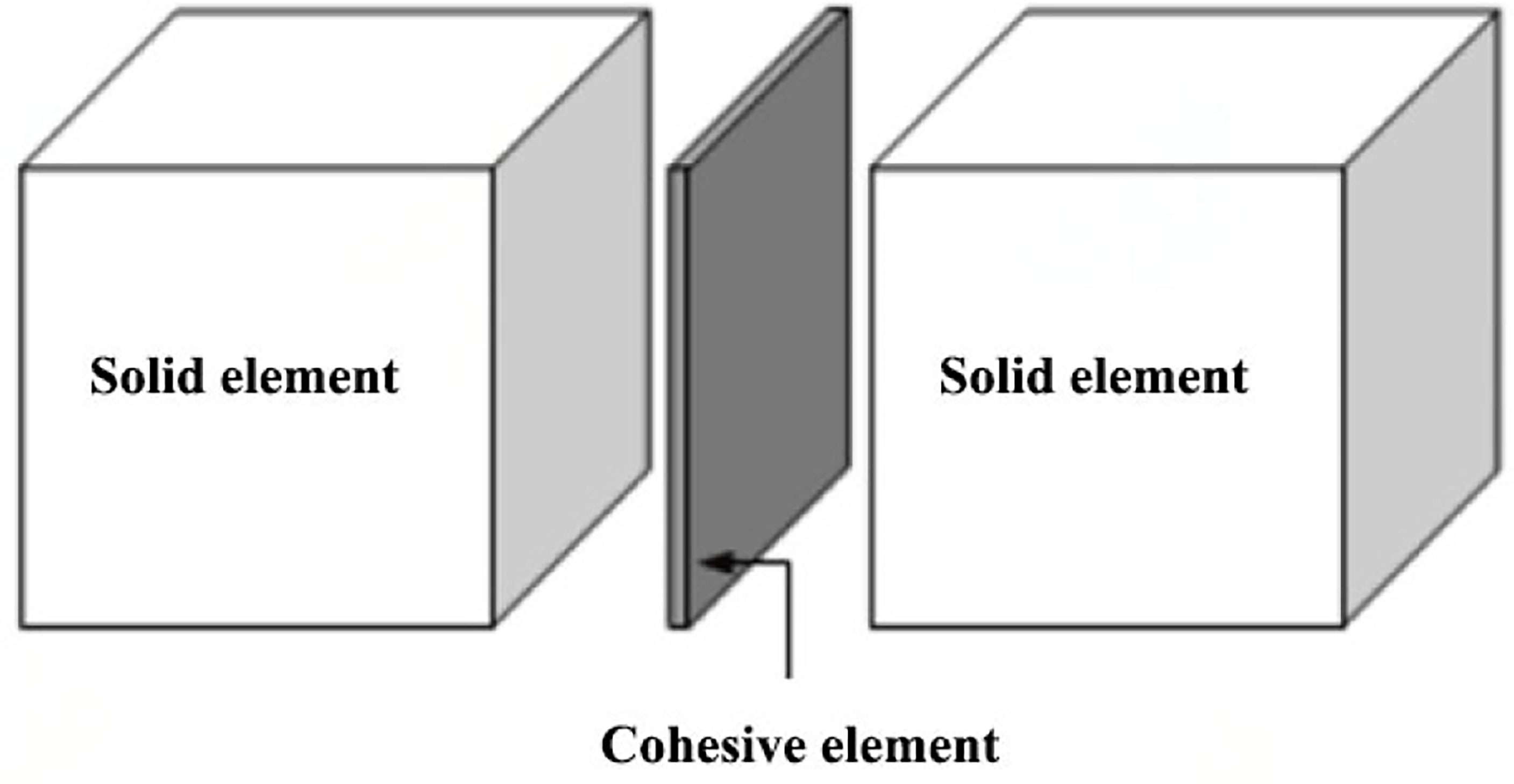
Figure 1 The cohesive element method (Hillervborg et al., 1976).

The cohesive element adopts the cohesive force constitutive model, and the failure of the element follows the traction force–separation displacement failure criterion. Three commonly used traction force–separation displacement curves, namely, bilinear softening, exponential softening, and trapezoidal softening, are shown in Figure 2. The traction force–separation displacement curve is mainly determined by fracture energy, fracture strength, and curve forms above. The area formed by the curves and the coordinate axis is the maximum energy required for the failure of the cohesive element, that is, the fracture energy.

FIGURE 2

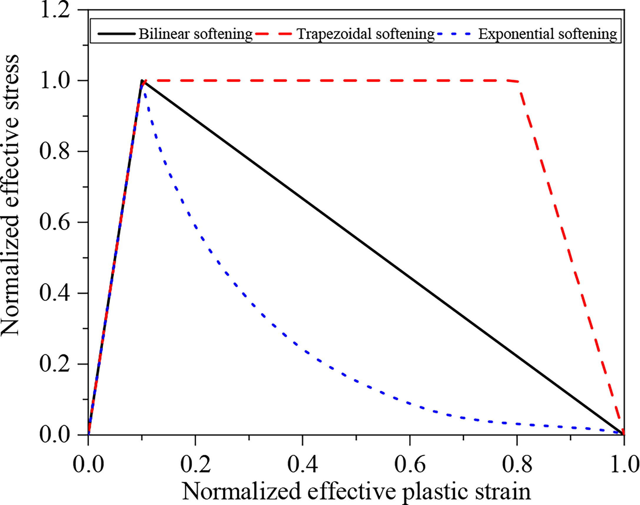
Figure 2 Cohesive element failure criterion models.

The relationship between the traction force and the separation displacement of the linear softening model can be expressed as:

$\begin{array}{ll}T=\{\begin{array}{c}\frac{T_0}{{\delta }_n^1}{\delta }_n,0\le {\delta }_n{\delta }_n^1\\ \frac{T_0}{({\delta }_n^f-{\delta }_n^1)}({\delta }_n^f-{\delta }_n),{\delta }_n^1\le {\delta }_n{\delta }_n^f\\ 0,{\delta }_n\ge {\delta }_n^f\end{array}& (8)\end{array}$

$\begin{array}{ll}S=\{\begin{array}{c}\frac{S_0}{{\delta }_n^1}{\delta }_{\tau },0\le {\delta }_{\tau }{\delta }_{\tau }^1\\ \frac{S_0}{({\delta }_{\tau }^f-{\delta }_{\tau }^1)}({\delta }_{\tau }^f-{\delta }_{\tau }),{\delta }_{\tau }^1\le {\delta }_{\tau }{\delta }_{\tau }^f\\ 0,{\delta }_{\tau }\ge {\delta }_{\tau }^f\end{array}& (9)\end{array}$

where T and S are tensile and shear stresses, respectively; T₀ and S₀ are the tensile and shear critical stresses, respectively; δ_n and δ_τ are separation displacements for tensile and shear fracture, respectively; ${\delta }_n^1$ and ${\delta }_{\tau }^1$ are the corresponding tensile and shear separation displacements at this time step, respectively; and ${\delta }_n^f$ and ${\delta }_{\tau }^f$ are the maximum separation displacements for tensile and shear fracture, respectively.

2.3.2 Sea ice constitutive model

For the solid ice elements, in order to reflect the generation and expansion of ice micro-cracks in the interaction between ice and OWTs, a homogenized elastic–plastic linear softening constitutive model is adopted in the presented study. The constitutive relationship of ice is shown in Figure 3. The material behaves elastically until the sea ice reaches yield strength. After reaching the yield point σ_c , the ice material begins to enter the linear softening stage, which means that with the increase of plastic strain, the effective stress is greatly reduced, and the sea ice is more easily crushed. Furthermore, when the failure strain is reached, ϵ_f , the sea ice elements are completely broken. The failure strain is used to control the failure deletion of solid ice elements in LS-DYNA and can be expressed as:

$\begin{array}{ll}{ϵ}_f={ϵ}_0+{(\frac{P}{{10}^8}-0.6)}^2& (10)\end{array}$

where ϵ₀ is the initial strain, which can be adjusted according to the ice test data. Based on the research results of the Norwegian University of Science and Technology, such parameter is selected as 0.01; P is the hydrostatic pressure.

FIGURE 3

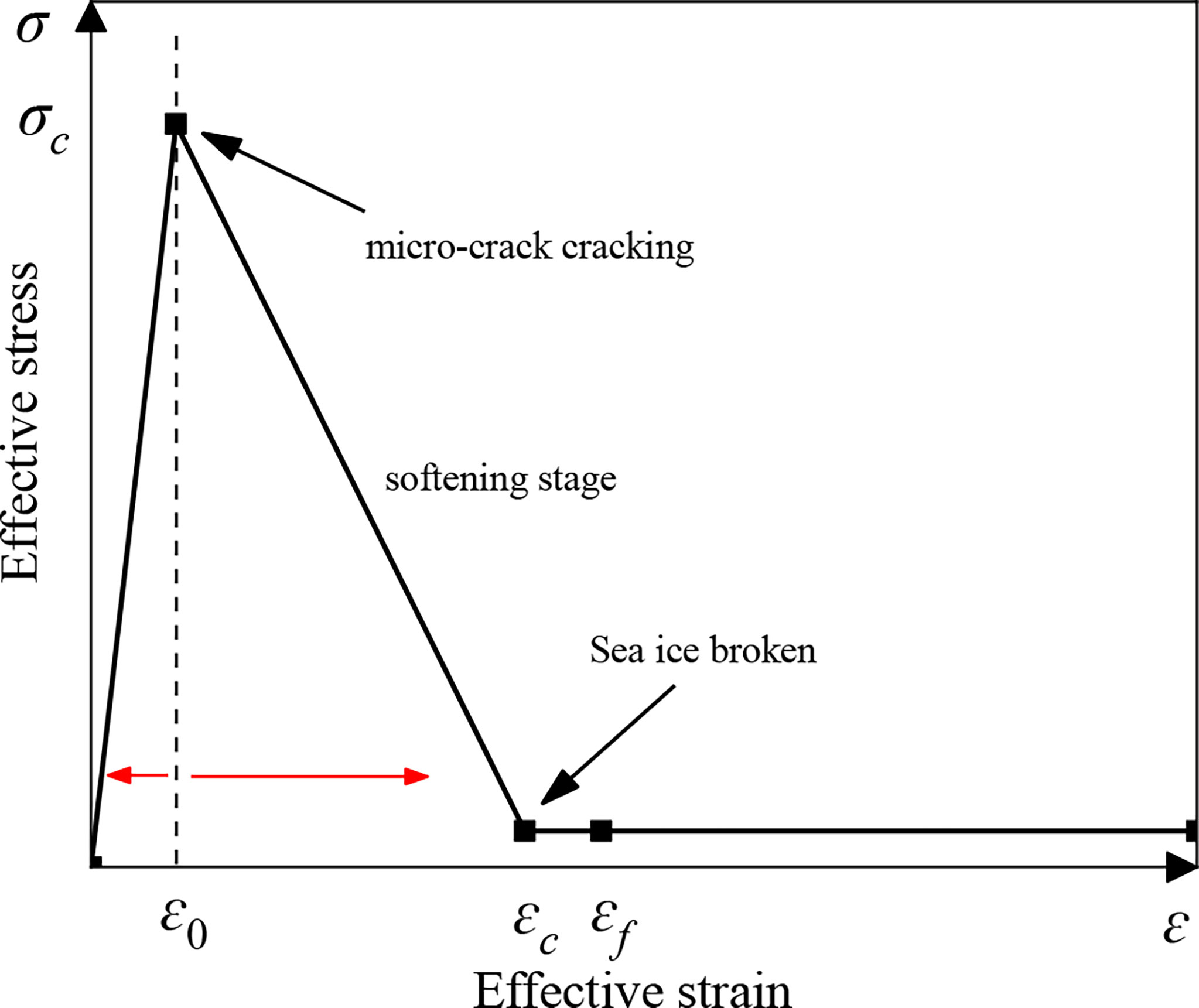
Figure 3 Ice solid element constitutive model.

Concurrently, considering the temperature effect and the sensitivity of ice strength to hydrostatic pressure, the Tsai-Wu failure criterion (Derradji-Aouat, 2003) is an effective criterion for describing the bending failure of sea ice, which can reflect the tension, compression, and shear of the ice element in the three-dimensional stress space. Meanwhile, the Tsai-Wu failure criterion is adopted as the criterion for ice crack initiation and propagation, which can be re-developed through the LS-DYNA user-defined subroutine. The Tsai-Wu failure criterion can be defined as:

$\begin{array}{ll}f=J_2-(b_0{+b}_1{P+b}_2{P}^2)=0& (11)\end{array}$

where, b₀, b₁, and b₂ are the constant coefficients obtained for fitting data from a triaxial experiment; and J₂ is the deviatoric stress, which is written as:

$\begin{array}{ll}{J}_2=\frac{1}{6}\left[{({\sigma }_x-{\sigma }_y)}^2+{({\sigma }_x-{\sigma }_z)}^2+{({\sigma }_y-{\sigma }_z)}^2\right]& (12)\end{array}$

where σ_x , σ_y , and σ_z are the first, second, and third principal stresses, respectively.

3 Numerical model of the interaction between ice and OWTs

3.1 Structural parameters of OWTs

Based on the DTU 10 MW baseline OWT (Velarde and Bachynski, 2017) proposed by the Technical University of Denmark (DTU) in cooperation with Vestas Company, an ice–OWT interaction model is established to conduct the dynamic response of OWT under wind and ice. As shown in Figure 4, the DTU 10 MW OWT is mainly composed of a rotor nacelle assembly (RNA), a supporting structure, and a pile foundation. The height from the hub to the water surface is 119 m, and the design water depth is selected as 20 m. The main parameters are shown in Table 1.

FIGURE 4

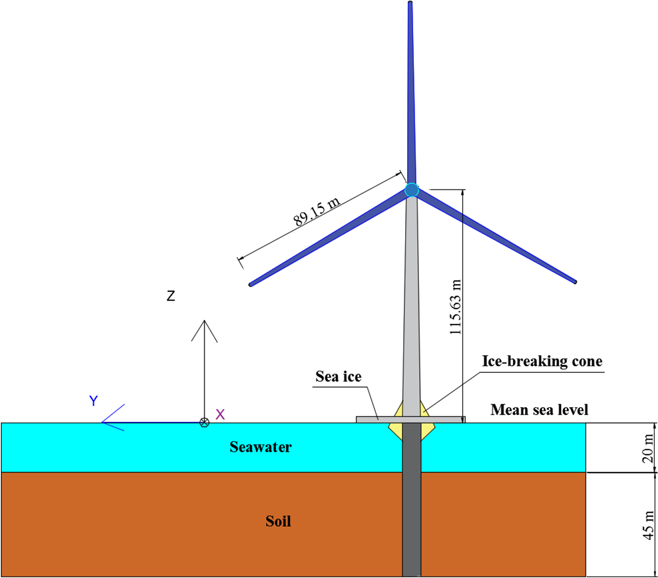
Figure 4 Schematic diagrams of the DTU 10 MW OWT (Velarde and Bachynski, 2017).

TABLE 1

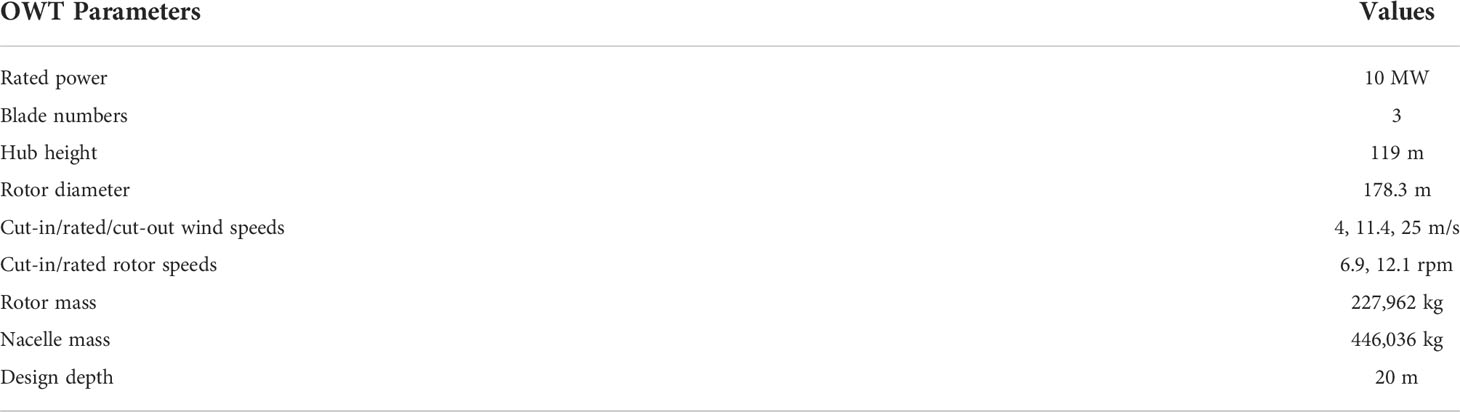
Table 1 Main specifications of the DTU 10 MW OWT (Velarde and Bachynski, 2017).

3.2 Sea ice model parameters

Traditional ice solid elements are modeled with eight-node hexahedral elements. However, for the bending failure of ice, the hexahedral element mesh shall result in breaking paths larger than the actual ice crack length, which can lead to additional dissipation of fracture energy with a non-negligible effect on the simulation results. Therefore, in this study, the six-node regular triangular prism meshing method is used to simulate the ice fracture and accumulation phenomena, as shown in Figure 5.

FIGURE 5

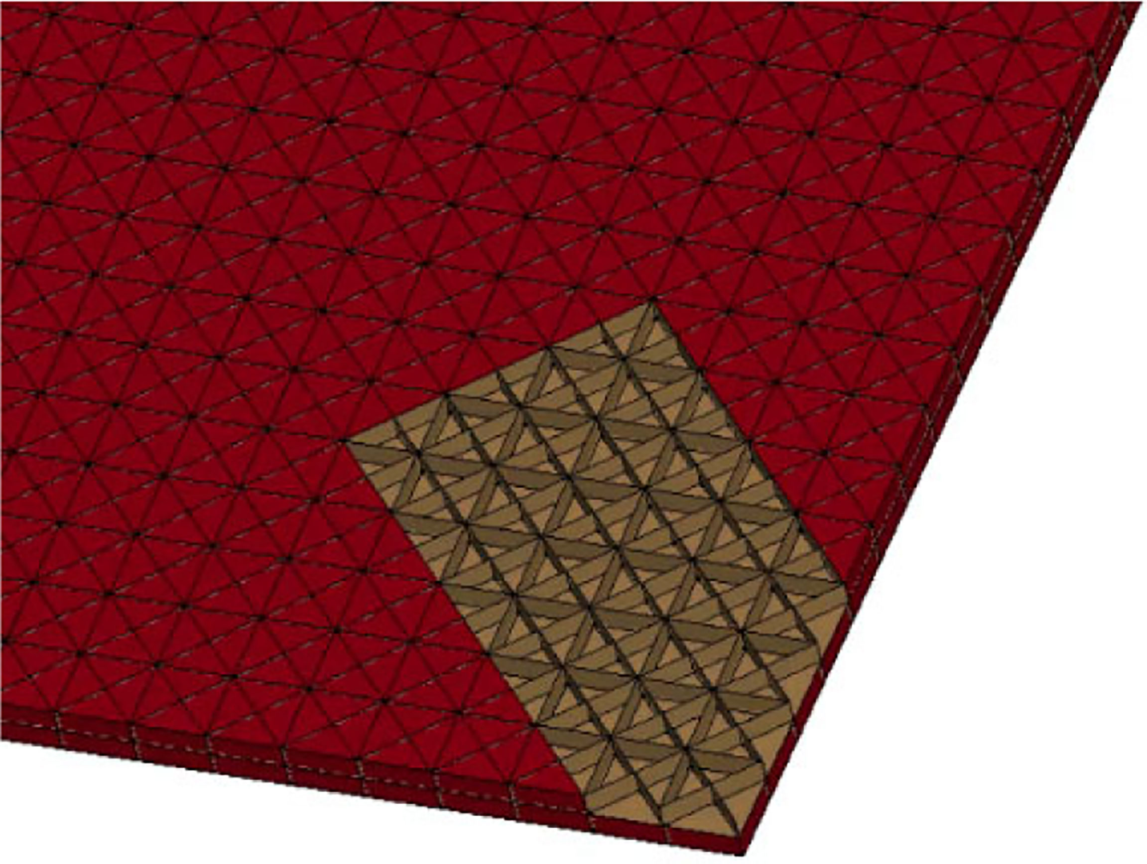
Figure 5 Sea ice finite element-cohesive element model.

The constitutive parameters of sea ice materials are affected by many factors. In this paper, the parameters of the elasto-plastic constitutive model of sea ice are determined based on the relevant research on the physical and mechanical properties of ice materials at home and abroad, and the effects of temperature, salinity, and porosity of sea ice on the properties of sea ice are considered, as shown in Table 2. Furthermore, Timco and Weeks (2010) obtained the tensile and shear rupture strengths of cohesive elements based on experimental data. In addition, Dempsey et al. (1999) carried out experimental studies on thick ice layers, and the fracture toughness values obtained showed that the fracture energy of ice ranges from 1 to 40 N/m. Based on the above research results, the parameters of the ice cohesive element are selected, as tabulated in Table 2.

TABLE 2

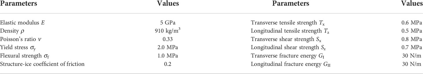
Table 2 Main material parameters of ice (Timco and Weeks, 2010).

In order to avoid the influence of the size of the ice sheet on the bending failure of the ice element in the contact area, and considering the calculation efficiency, the size (length × width: 36 m × 20 m) of the ice sheet is determined based on the elastic foundation beam theory. The side that collided with the ice sheet is set as a free boundary condition, and the other three sides only constrain the y-direction degree of freedom and set a non-reflection boundary condition to exclude the influence of the reflection of stress waves from the boundary on the numerical simulation results. Meanwhile, an elastic base plate is established to simulate seawater buoyancy, as shown in Figure 6.

FIGURE 6

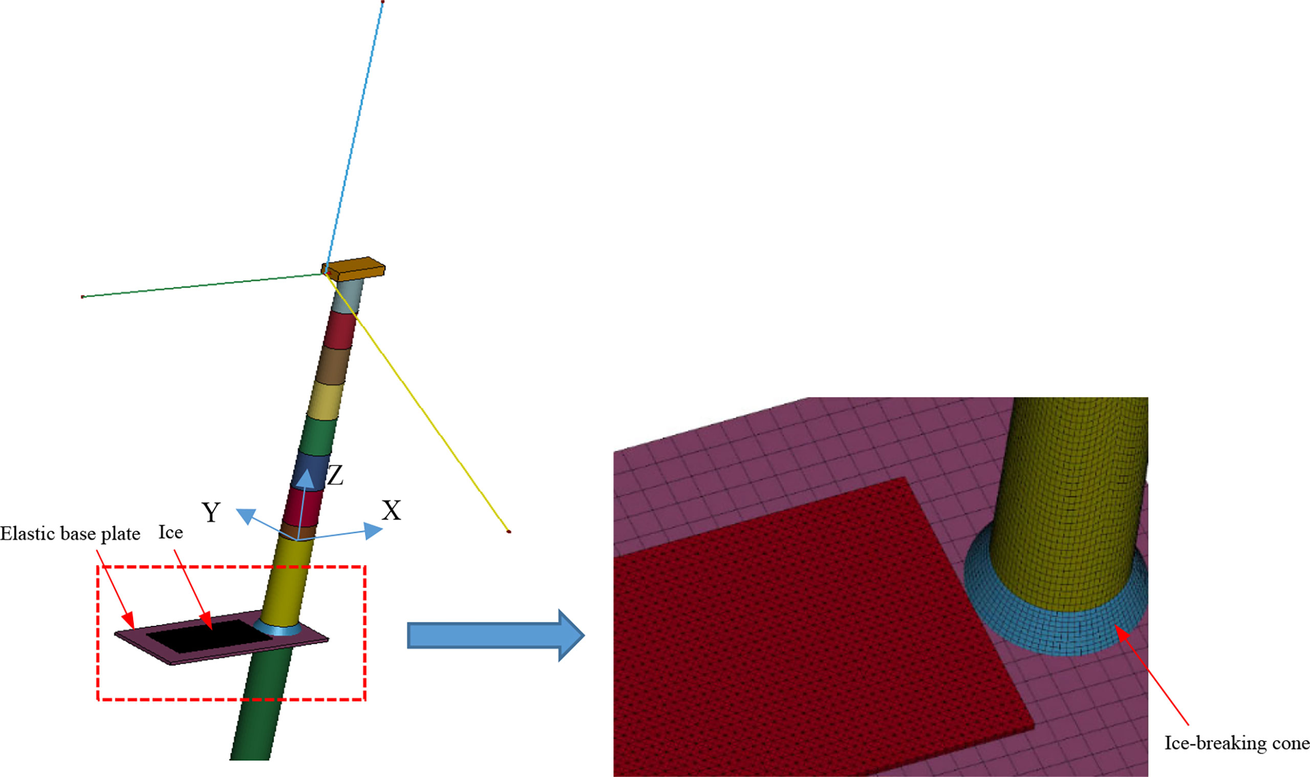
Figure 6 Ice–OWT interaction coupling model.

3.3 Pile–soil interaction parameters

According to the soil parameters in Ref (Yang et al., 2020)., the site soil conditions shown in Figure 7 are adopted in the monopile OWT. Soil conditions are designed as sandy soil with a depth of 45 m. The internal friction angle is 36°, and the saturation weight is selected as 20 kN/m³.

FIGURE 7

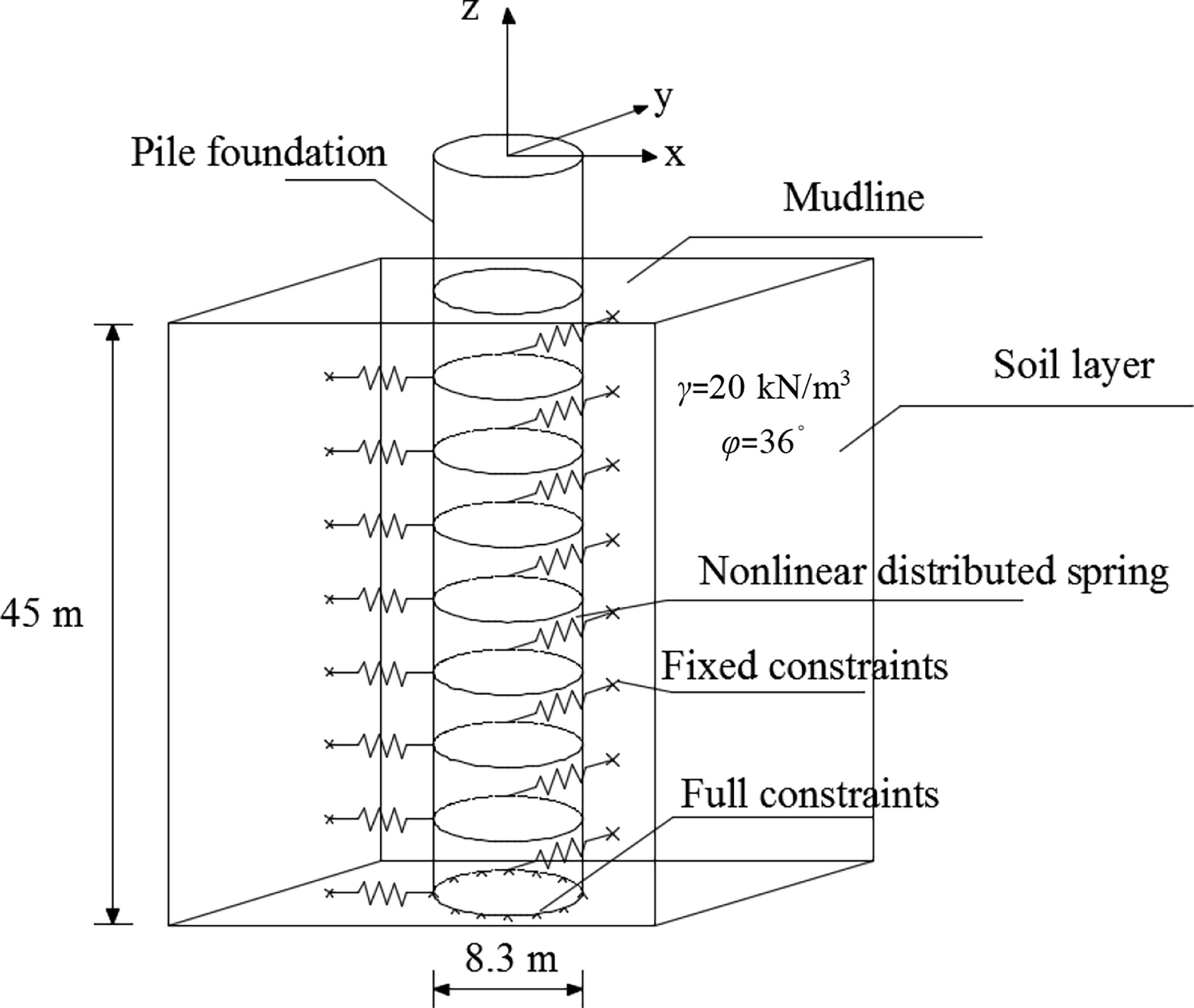
Figure 7 Pile–soil interaction model based on nonlinear distributed springs.

During the interaction between sea ice and OWTs, the pile foundation of OWT is mainly affected by the horizontal direction, and the displacement variations caused by the vertical pile side friction can be ignored. Sequentially, based on the p–y curve method, a nonlinear distributed spring in the horizontal direction is used to simulate the pile–soil interaction under the combined action of wind and ice, as shown in Figure 7. At different depth positions in the horizontal x, y direction, one node of the distribution spring is connected to the pile foundation, and the other node is set as the fixed end.

3.4 Contact settings and hourglass control

In order to ensure that the initial contact is eliminated between the OWT substructure and ice, an initial collision distance of 0.1 m is set in the fully coupling interaction model. The contact for eroding surface to surface is applied to the interaction of ice and OWT. However, in order to reduce the computation time, the contact between ice fragments adopts eroding single surface contact. Simultaneously, the contact stiffness is increased by four to five times to reduce unnecessary penetration between ice and the OWT substructure. It is found that such contact stiffness can obtain better numerical simulation results through tests (Liu et al., 2022).

Thereafter, the hourglass mode is a non-physical zero-energy deformation mode that results in zero strain and stress, which can cause errors in the calculation results in LS-DYNA. When the hourglass energy exceeds 10% of the total internal energy of the structure, the analysis results can be considered invalid. Therefore, the hourglass phenomenon needs to be effectively controlled in the ice–OWT interaction. This paper found that the rigid hourglass control can effectively suppress the hourglass phenomenon compared with the viscous hourglass control by conducting a comparative study on the hourglass control.

4 Calculation results and discussion

4.1 Design of load cases

Considering the pile–soil interaction, this paper focuses on the effects of different ice speeds and cone angles on the motion response of the DTU 10 MW OWT under the wind and ice loads. Based on the relevant sea conditions in the Bohai Sea and the requirements of the IEC-61400-1 specification (IEC, 2012), and combined with the cut-in and cut-out wind speeds of the DTU 10 MW wind turbine, the typical combined wind and ice conditions are selected as shown in Table 3.

TABLE 3

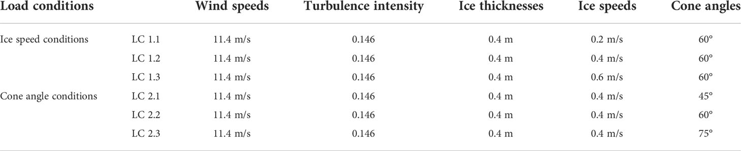
Table 3 Designed combined load conditions.

The average reference wind speed at the hub height of the OWT is a rated wind speed of 11.4 m/s and a specified turbulence intensity of 0.146 is selected in the presented study. Using the IEC Kaimal turbulence model and exponential coherence model, a turbulent wind field with a time step of 0.02 s is generated by TurbSim (Kilcher, 2012). The time-domain variation curve of wind speed at the hub height is shown in Figure 8. In addition, the cone angle conditions (LC 2.1–LC 2.3) only changed the cone angle by keeping the identical diameter of the water surface of the cone, that is, ensuring a uniform collision position of sea ice, as shown in Figure 9.

FIGURE 8

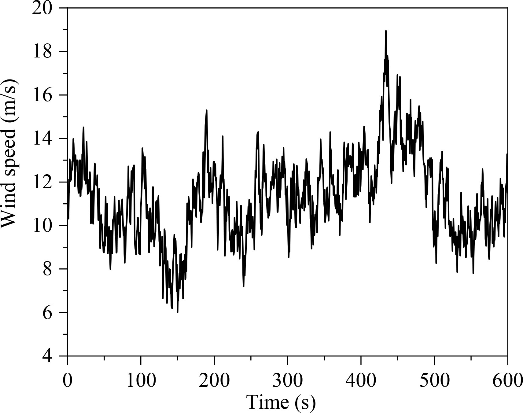
Figure 8 Synthesized stochastic wind speeds based on IEC Kaimal turbulence model.

FIGURE 9

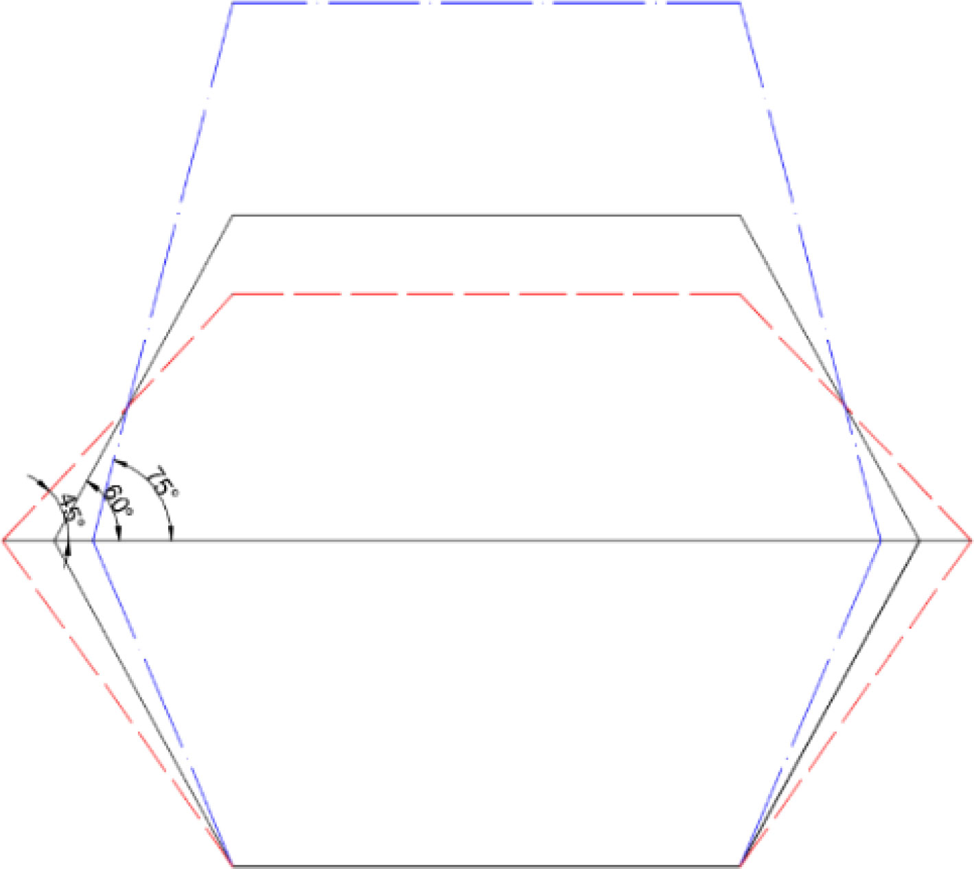
Figure 9 Schematic diagram of ice-breaking cone angle based on same collision location.

4.2 Sea ice bending failure and ice force verification

4.2.1 Bending failure mode of ice

Figure 10 shows the simulation results of ice bending failure and ice fragment accumulation effect under colliding with a constant velocity of 0.4 m/s. When the sea ice makes initial contact with the cone, the front of sea ice crawls a short distance along the cone. As the bending stress of the sea ice reaches its bending strength, tiny radial cracks first appear on the ice surface. This is due to the deletion of cohesive elements at the front of ice, resulting in radial failure exhibiting a non-simultaneous failure mode subjected to non-uniform forces. Furthermore, the crushed ice broken from the ice floe shall climb up and down slightly on the cone surface and remain at the height of the water level under the combinations of gravity and the buoyancy provided by the elastic base in Figure 6. Consequently, the accumulation phenomenon of ice fragments can be observed. Finally, with the continuous occurrence of collisions and the generation of broken annular cracks, the ice fragments gradually climb, slide, accumulate, and clear on the ice front until equilibrium. At this point, the cone completely invades the ice sheet. Therefore, in the process of the fully ice–OWT interaction, the dynamic ice loads on the ice-breaking cone can be divided into the direct action of sea ice on the cone surface and the contact action of accumulated ice fragments.

FIGURE 10

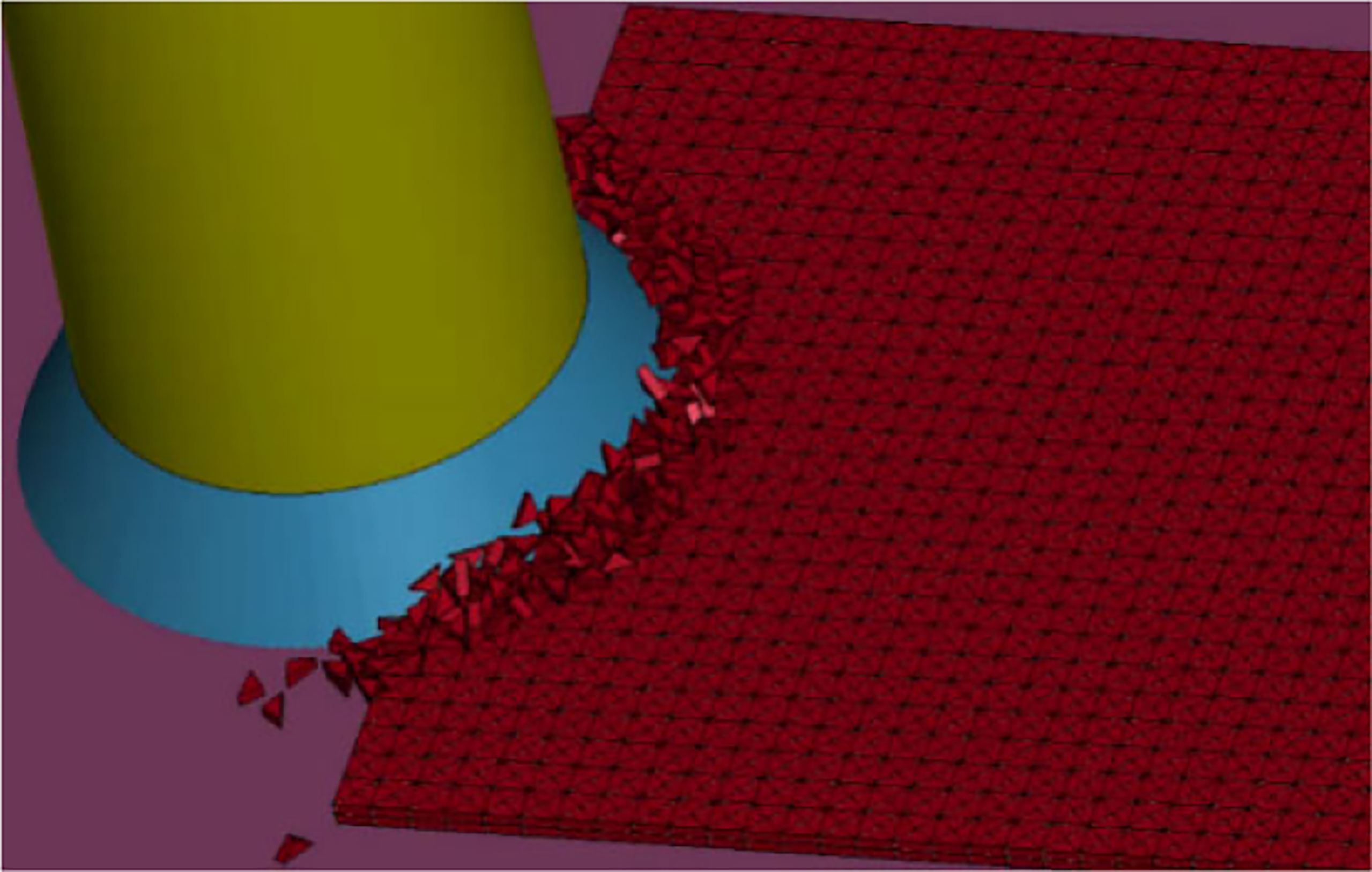
Figure 10 Bending failure mode of the sea ice model.

Furthermore, according to the degree of intrusion into the ice sheet by the OWT structure, the effective stress distribution of ice is illustrated in Figure 11. As indicated in the figure, in the early stage of contact collision, cracks are initiated and the fractured ice elements begin to separate from the ice sheet. Then, as the OWT structure intrudes, the stress wave exhibits a circular spread.

FIGURE 11

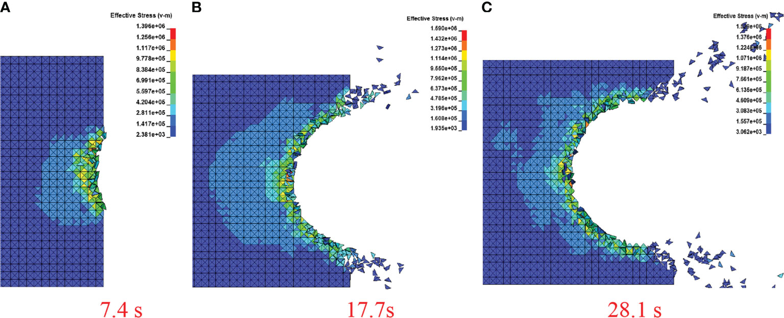
Figure 11 Ice stress distribution at different time steps. (A) at 7.4 s. (B) at 17.7 s. (C) at 28.1 s.

4.2.2 Ice force verification

The numerical calculation results of the ice force in the presented study are compared with the three-dimensional horizontal and vertical static ice force calculation models of the cone structure of Ralston (1980) and Croasdale and Cammaert (1994) to verify the accuracy of the numerical simulation. The static ice force calculation models are expressed as

$\begin{array}{ll}{F}_H^R=A_4[{\text{A}}_1{\sigma }_f{h}^2+{\text{A}}_2{\rho }_w{\text{g}h\text{D}}^2+{\text{A}}_3{\rho }_w\text{g}h({\text{D}}^2-{\text{D}}_T^2)]& (13)\end{array}$

$\begin{array}{ll}{F}_V^R{\text{=B}}_1{F}_H+B_2{\rho }_{w}gh({\text{D}}^2-{\text{D}}_T^2)& (14)\end{array}$

$\begin{array}{ll}{F}_H^C=C_1\text{D}{\sigma }_f{({\rho }_w{\text{g}h}^5/E)}^{0.25}+C_2{h}_{R}h\text{D}{\rho }_i\text{g}& (15)\end{array}$

$\begin{array}{ll}{F}_V^C=F_H/\varsigma & (16)\end{array}$

where the superscripts R and C represent the Ralston and Croasdale ice force models, respectively; F_H and F_V are the horizontal and vertical loads, respectively; D is the diameter of the cone at the waterline; D_T is the diameter of the top of the cone; ρ_i is the sea ice density; h is the sea ice thickness; h_R is the ice climbing height; E is the elastic modulus of the sea ice; A₁, A₂ are dimensionless coefficients depending on the ice thickness and flexural strength; and A₃, A₄, B₁, B₂, C₁, and C₂ are the dimensionless coefficients that depend on the cone angle and the ice-cone friction coefficient, respectively.

Figure 12 shows the dynamic ice force time history of the collision between an ice sheet with an ice velocity of 0.4 m/s, an ice thickness of 0.4 m, and an ice-breaking cone with a cone angle of the 60°. The dynamic ice force with obvious fluctuations can be distinctly observed from the figure. This is because the ice floes have been going through a cyclic process of "contact deformation–fracture failure–accumulated climbing–ice fragment removal–contact deformation". Under the compressive stress and bending stress, the amplitudes of ice force gradually increases. Subsequently, the ice loads are unloaded due to the failure deletion of the cohesive elements. Furthermore, it can be seen from Figure 12A that the simulation results of the presented study and the horizontal maximum ice force values calculated by the Ralston model and the Croasdale model are 1.360 MN, 1.427 MN, and 0.829 MN, respectively. The certain difference in the calculation results of the two model formulas can be discovered from the figure, and the Croasdale model has the smallest calculation result for ice force. Moreover, simulation results of the horizontal ice force amplitude in the presented study are between the Ralston model and the Croasdale model, and the relative error with the Ralston model is the smallest, which is only 15.35%. However, for LC 2.3 of the combined load case with a cone angle of 75°, the maximum error of the horizontal ice force reaches 92.86%, which indicates that the static ice force model used in the study of ice-induced vibration of OWTs with large cone angles shall significantly overestimate the ice force results. This difference is mainly due to the discrepancies between the selection of physical and mechanical parameters of sea ice in the coupling interaction model of ice–OWT and the theoretical models for ice force. In addition, the pile–soil interaction is a factor not considered in the theoretical models, and the influence of the pile–soil interaction cannot be ignored in the dynamic response analysis of OWTs. The calculation of relative error Δ is shown in Eq. (17).

$\begin{array}{ll}\Delta =(\frac{\left|X_{numerical}-X_{theoretical}\right|}{X_{numerical}})\times 100\%& (17)\end{array}$

where X_numerical is the numerical simulation result in the presented study and X_theoretical is the result calculated by ice force theoretical models.

FIGURE 12

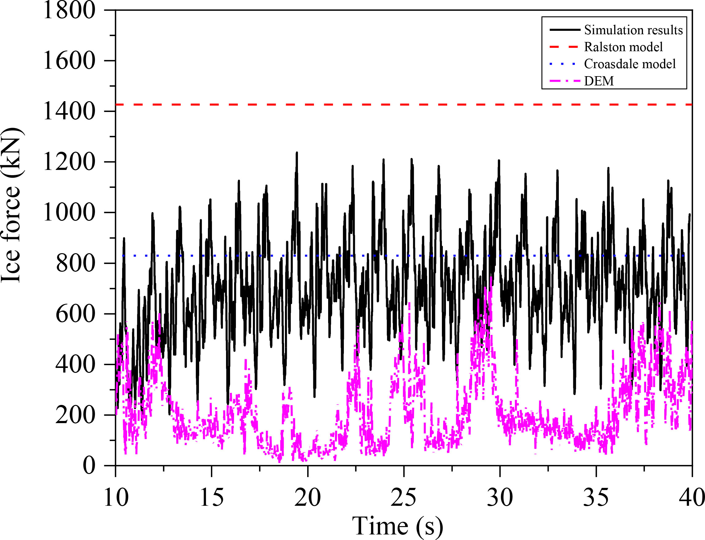
Figure 12 Comparison of dynamic ice load calculation with CEM, DEM, and static ice force models.

The amplitude of dynamic ice force is not sensitive to the variations of ice speeds observed from the statistics of horizontal and vertical dynamic ice loads in Tables 4, 5. In the LC 1.1 load case, the simulated dynamic ice force amplitude is 1.226 MN, and the relative error with the Ralston model is 16.39%. In the load cases of LC 1.2 and LC 1.3, the above relative errors are 15.35% and 4.93%, respectively. On the other hand, as the cone angle increases, the ice force amplitude increases significantly. Taking the 60° cone angle as an example, the horizontal ice force amplitude when the 75° cone angle is used can obtain 1.681 MN, which is significantly larger than the 60° cone angle condition of LC 2.2. Furthermore, as noted from Table 5, consistent with the variation law of the horizontal dynamic ice loads, the vertical dynamic ice loads increase slightly with the increase of the ice speed. However, with the increase in cone angles, the dynamic ice load amplitude decreases, which is consistent with the results calculated by the Croasdale model. It is demonstrated that the more obvious reduction of the horizontal dynamic ice force of the ice-breaking cone can be caused by the smaller cone angles. However, it shall lead to the increase of the vertical ice dynamic force, which is prominently unfavorable for the ice-breaking cone.

TABLE 4

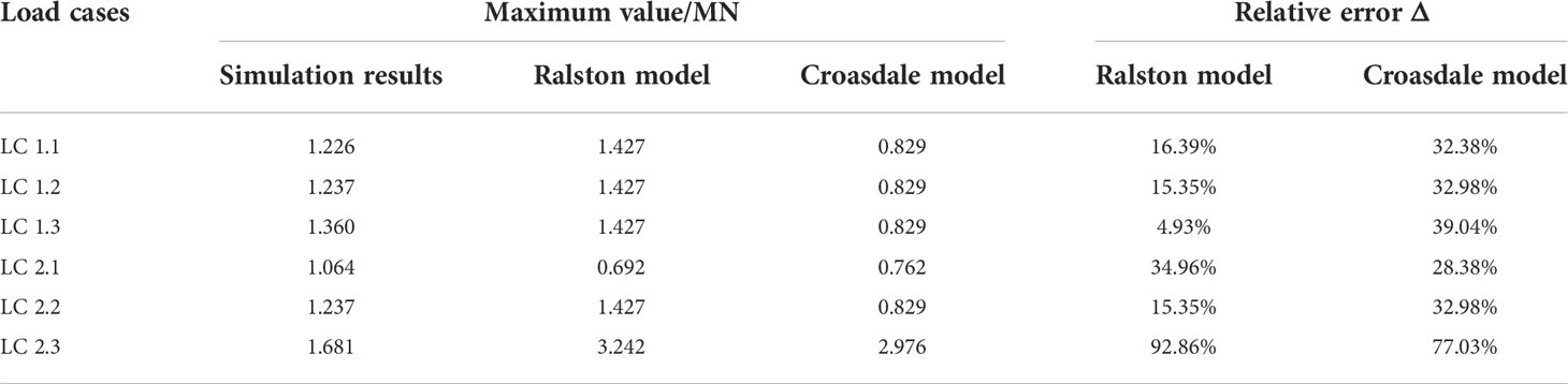
Table 4 Comparisons of horizontal ice load statistics.

TABLE 5

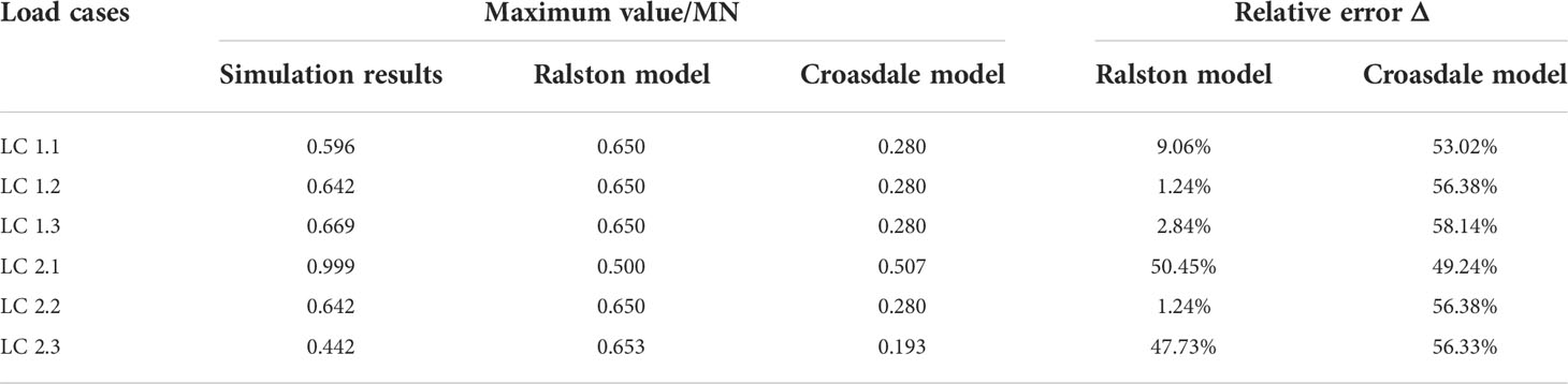
Table 5 Comparisons of vertical ice load statistics.

Furthermore, the dynamic ice force comparison results on the basis of DEM can be found in Figure 12. For the bending failure of ice, when applying the DEM to dynamic ice load calculations, the magnitude of dynamic ice force is less than that of CEM. For example, the maximum ice force based on DEM and CEM is 0.753 MN and 1.237 MN, respectively. In addition, by comparing the DEM results, static ice force calculation models are more conservative. This is mainly because there are many limitations and differences in the parameter selection of sea ice and the OWT structure that affect the basic assumptions of sea ice models and the results of numerical simulations. Meanwhile, the calculation parameters of DEM, such as the number of particle layers, stiffness, and bond strength, also need to be further determined. Moreover, since sea ice failure relies on small-sized cohesive spherical particles in DEM, differences in ice failure paths and crack lengths shall also lead to discrepancies of dynamic ice forces.

4.3 Ice-induced vibration of OWT structures with cones

Figures 13A, B show the time-history curves of the displacement response at the tower top under different ice velocities and cone angles, respectively. From Figure 13A, it can be found that the ice speed has little effect on the structural motion response of the OWT, especially for the operating status of the OWT in this study. In addition, relative to the ice velocity, the obvious differences are depicted in the displacement time-history curves under the three cone angle conditions, and the difference in the above displacement amplitudes reaches 0.13 m, as shown in Figure 13B. In order to further evaluate OWT vibrations under ice and wind loads, tower top acceleration statistics are listed in Table 6. As noted from the table, the same results can also be observed; that is, ice speeds have little effect on acceleration amplitude. However, as the cone angle increases, the acceleration amplitude at the tower top increases. For example, the acceleration amplitude of the OWT with 75° cone can exceed 2.4 m/s². Moreover, the acceleration fluctuations are more consistent under different ice speeds and cone angles by comparing the standard deviation.

FIGURE 13

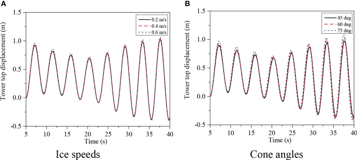
Figure 13 Histories of tower top displacements under selected wind-ice cases. (A) Ice speeds (B) Cone angles.

TABLE 6

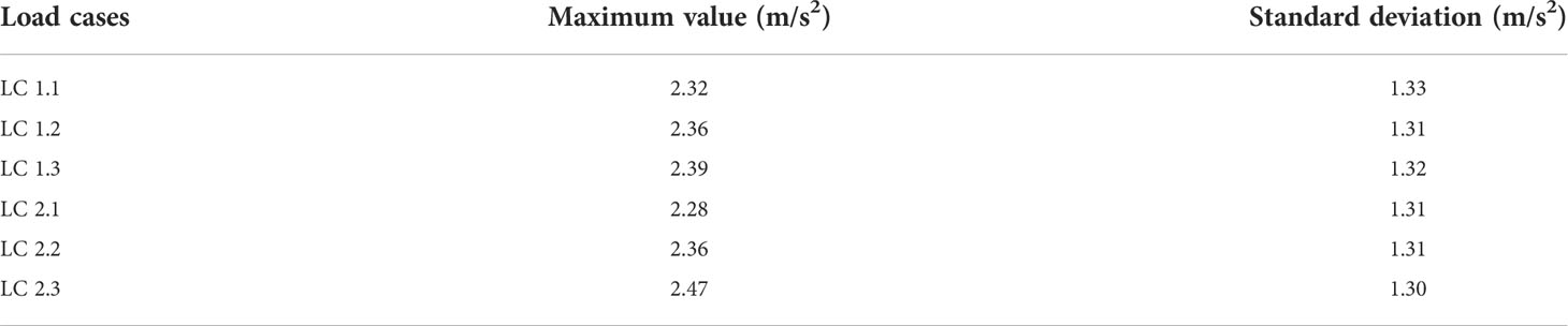
Table 6 Comparisons of tower top acceleration statistics.

To further illustrate the discrepancies in the vibration characteristics at the tower top of the OWT, the frequency domain displacement responses at the tower top under the corresponding sea ice conditions are shown in Figure 14. In the frequency domain, the tower top displacement is mainly affected by the fundamental frequency of the overall structure of 0.246 Hz. It should be noted that since the quality variations of the ice-breaking cone are induced by the cone angles in Figure 9, the fundamental frequencies of the OWT with three ice-breaking cones are slightly different, which are 0.247 Hz, 0.246 Hz, and 0.245 Hz, respectively, as shown in Figure 14B. In addition, the increase in the weight of the ice-breaking cone shall cause the fundamental frequency of the OWT to decrease, which shall lead to the OWT structure resonance more easily. Meanwhile, considering the influence of the cone angle on the dynamic ice loads in the horizontal and vertical directions, it is recommended to select the cone angle as 60°.

FIGURE 14

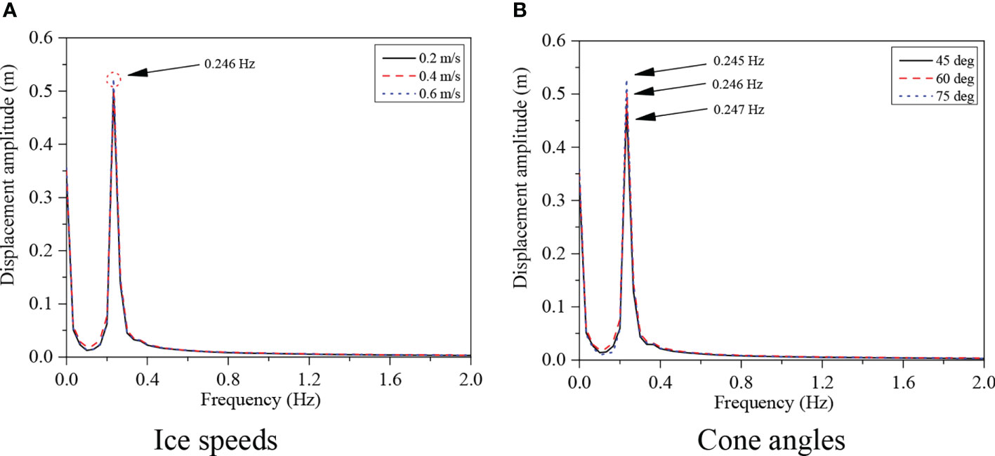
Figure 14 Fourier amplitudes of tower top displacements under selected wind-ice cases. (A) Ice speeds (B) Cone angles.

4.4 Damage analysis of the ice-breaking cone

Based on the CEM, the Von-Mises effective stress and pressure of the conical OWT structure under the sea ice can be obtained through the established ice–OWT interaction coupling model, as shown in Figure 15. The annular spread of stress at the collision position can be observed. Moreover, the remarkable increasing trend of damage distribution with the increasing of the cone angles is indicated in the figure. The main reason for such result is that the increase of the cone angle leads to a larger contact area between the ice and the cone surface. Concurrently, it can be seen from Figure 16 that the stress distribution corresponds to the pressure distribution, and the maximum pressure is the region with the maximum Von-Mises effective stress.

FIGURE 15

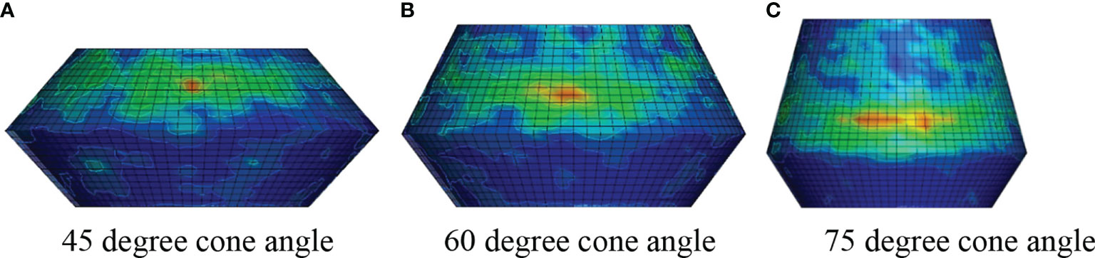
Figure 15 Conical structure Von-Mises effective stress distribution. (A) 45° cone angle (B) 60° cone angle (C) 75° cone angle.

FIGURE 16

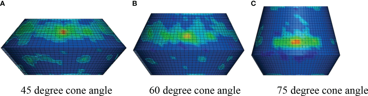
Figure 16 Pressure distribution of cone structure. (A) 45° cone angle (B) 60° cone angle (C) 75° cone angle.

The variation trends of Von-Mises effective stress and pressure with different cone angles are shown in Figure 17. It can be seen from the comparison of the figures that the cone angle has a great influence on the stress. With the increase of the cone angle, the Von-Mises effective stress and pressure show an increasing trend, which is also consistent with the dynamic ice loads and the dynamic response of the OWT structure. Furthermore, the comparison results show that the maximum Von-Mises effective stress is 186 MPa, which does not reach the yield strength of the steel material of 355 MPa; that is, the OWT structure is in the elastic deformation stage during the ice–OWT interaction.

FIGURE 17

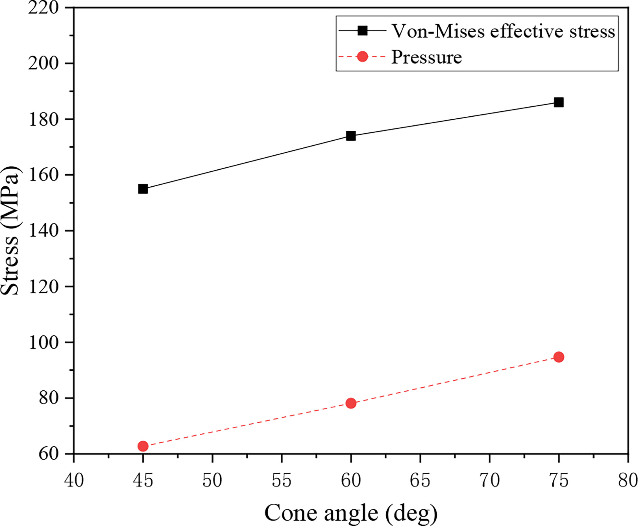
Figure 17 Maximum Von-Mises effective stress of pyramidal structures under different taper angles.

Conclusion

In this paper, nonlinear distributed springs are used to simulate the pile–soil interaction of OWTs, and based on the CEM, an ice–OWT interaction model with ice-breaking cones is established. Furthermore, based on the secondary development of LS-DYNA, the Tsai-Wu yield criterion and empirical failure formula are used to describe the failure and failure modes of sea ice, and the bending failure process of sea ice is simulated. According to the established interaction coupling numerical simulation model, the analysis on the motion response and strength of the OWT with cone under the combined wind and ice are carried out. The main conclusions of the research are as follows:

1. Based on the CEM, the cohesive element model is combined with the finite element constitutive model to carry out numerical simulation research on the coupled interaction between ice and OWTs. Compared with the Ralston ice force model and the Croasdale ice force model, the result shows that the adopted method in the presented study can simulate the bending failure behavior of sea ice well, especially regarding the failure of ice elements and the accumulation of ice fragments consistent with actual field conditions.

2. With the increase in ice velocity, the motion response of OWTs is increasing. However, the ice velocity has little effect on the dynamic ice loads and the structural motion response of the OWTs, especially for the operating OWT with the pile–soil interaction.

3. The ice-breaking cone angle has a significant impact on the dynamic ice loads and the structural motion response of OWTs. As the cone angle increases, the magnitude of the horizontal ice load increases significantly; however, for the vertical ice load, the magnitude shows a decreasing trend. This is mainly because variations in the cone angle change the pattern of sea ice destruction. In addition, the increased weight of the ice-breaking cone may lead to the resonance of OWT. Therefore, considering the pile–soil interaction, it is suggested that the optimal ice-breaking cone angle of the OWT under the operating state is 60°.

4. The remarkable discrepancies in the damage of the ice-breaking cone surface with different cone angles can be directly observed. The Von-Mises effective stress distribution is consistent with pressure distribution. With the increase of the cone angles, the stress damage area and effective stress amplitude are also positively correlated. However, the maximum Von-Mises effective stress is much smaller than the yield strength of the steel material. This indicates that the linear analysis of the OWT structure in the elastic range is also reasonable for the ice-conical OWT structure interaction process.

Data availability statement

The original contributions presented in the study are included in the article/supplementary material. Further inquiries can be directed to the corresponding author.

Author contributions

Conceptualization, WS, JZ and XL. Methodology, BW, YZL, and YL. Investigation, BW and YZL. Writing—first draft preparation, BW, YZL, JZ, and WS. Review and editing, WS and XL. Supervision, WS and XL. Project administration, JZ. Funding acquisition, WS and XL. All authors contributed to the article and approved the submitted version.

Funding

This research was supported by Key Laboratory of far-shore wind power technology of Zhejiang Province (ZOE2020003), Zhejiang Provincial Natural Science Foundation of China (LHY21E090001) and the National Natural Science Foundation of China (Grant Nos. 52001052, 51939002, 52071058, 52071301 and 51909238). And partially supported by Ministry of Industry and Information Technology (2020) g-275.

Conflict of interest

The authors declare that the research was conducted in the absence of any commercial or financial relationships that could be construed as a potential conflict of interest.

Publisher’s note

All claims expressed in this article are solely those of the authors and do not necessarily represent those of their affiliated organizations, or those of the publisher, the editors and the reviewers. Any product that may be evaluated in this article, or claim that may be made by its manufacturer, is not guaranteed or endorsed by the publisher.

References

Croasdale K. R., Cammaert A. B. (1984). An improved method for the calculation of ice loads on sloping structures in first-year ice. Hydrotech Constr. 28 (3), 174–179. doi: 10.1007/BF01545935

CrossRef Full Text | Google Scholar

Dempsey J. P., Adamson R. M., Mulmule S. V. (1999). Scale effects on the in situ tensile strength and fracture of ice. part II: first-year sea ice at resolute, NWT. Intentional J. Fract 95 (1-4), 347–366. doi: 10.1023/a:1018650303385

CrossRef Full Text | Google Scholar

Derradji-Aouat A. (2003). Multi-surface failure criterion for saline ice in the brittle regime. Cold Reg. Sci. Tech 36 (1-3), 470–470. doi: 10.1016/S0165-232X(02)00093-9

CrossRef Full Text | Google Scholar

Di S., Xue Y., Wang Q. (2017). Discrete element simulation of ice loads on narrow conical structures. Ocean Eng. 146 (1), 282–297. doi: 10.1016/j.oceaneng.2017.09.033

CrossRef Full Text | Google Scholar

DNV GL (2016). DNV GL-ST-0437: Loads and site conditions for wind turbines (Oslo, Norway: DNV GL).

Google Scholar

Gladman B. (2013). LS-DYNA keyword user's manual, volume Ⅱ, material models (Livermore, California: Livermore Software Technology Corporation).

Google Scholar

Hallquist J. (2006). LS-DYNA® theory manual. Livermore (Livermore, California: Livermore Software Technology Corporation), 3.

Google Scholar

Heinonen J., Rissanen S. (2017). Coupled-crushing analysis of a sea ice-wind turbine interaction-feasibility study of FAST simulation software. Ships Offshore Struct. 12 (7-8), 1–8. doi: 10.1080/17445302.2017.1308782

CrossRef Full Text | Google Scholar

Hillervborg A., Mod E. M., Petersson P. E. (1976). Analysis of crack formation and crack growth in concrete by means of fracture mechanics and finite elements. Cem Concr Res. 6 (6), 773–781. doi: 10.1016/0008-8846(76)90007-7

CrossRef Full Text | Google Scholar

IEC (2012). IEC 61400-1: Wind turbine-part 1: Design requirements (Geneva, Switzerland: IEC).

Google Scholar

Jang H. K., Kim M. H. (2021). Dynamic ice force estimation on a conical structure by discrete element method. Int. J. Nav Archit Ocean Eng. 13 (1), 136–146. doi: 10.1016/j.ijnaoe.2021.01.003

CrossRef Full Text | Google Scholar

Kilcher J. (2012). TurbSim user's guide (Draft version) (Golden, USA: National Renewable Energy Laboratory, Golden).

Google Scholar

Lan J. Y., Liu H. S., Lv Y. J. (2012). Dynamic nonliner parameters of soil in the bohai sea and their rationality. J. Harbin Eng. Univ. 33 (9), 1079–1085. doi: 10.3969/j.issn.1007-7043.201202036

CrossRef Full Text | Google Scholar

Liu Y. Z., Shi W., Wang W. H. (2022). Dynamic analysis of monopile-type offshore wind turbine under Sea ice coupling with fluid-structure interaction. Front. Mar. Sci. 9, 839897. doi: 10.3389/fmars.2022.839897

CrossRef Full Text | Google Scholar

Ralston T. D. (1980). Plastic limit analysis of sheet ice loads on conical structures, physics and mechanics of ice, 289–308.

Google Scholar

Ren Y., Vengatesan V., Shi W. (2022). Dynamic analysis of a multi-column TLP floating offshore wind turbine with tendon failure scenarios. Ocean Eng. 245, 110472. doi: 10.1016/j.oceaneng.2021.110472

CrossRef Full Text | Google Scholar

Shi W., Tan X., Gao Z. (2016). Numerical study of ice-induced loads and responses of a monopile-type offshore wind turbine in parked and operating conditions. Cold Reg. Sci. Tech 123, 121–139. doi: 10.1016/j.coldregions.2015.12.007

CrossRef Full Text | Google Scholar

Song M., Shi W., Ren A. R., Zhou L. (2019). Numerical study of the interaction between level ice and wind turbine tower for estimation of ice crushing loads on structure. J. Mar. Sci. Eng. 7 (12), 439. doi: 10.3390/jmse7120439

CrossRef Full Text | Google Scholar

Statoilhydro A. G., Bjerks M., Kühnlein W. (2009). In: Proceedings of the ASME 28th International Conference on Ocean, Offshore and Arctic Engineering, Honolulu, Hawaii, USA, May 31 - June 5. doi: 10.1115/OMAE2009-80164

CrossRef Full Text | Google Scholar

Timco G. W., Weeks W. F. (2010). A review of the engineering properties of sea ice. Cold Reg. Sci. Tech 60 (2), 107–129. doi: 10.1016/j.coldregions.2009.10.003

CrossRef Full Text | Google Scholar

Velarde J., Bachynski E. E. (2017). Design and fatigue analysis of monopile foundations to support the DTU 10 MW offshore wind turbine. Energy Proc. 137, 3–13. doi: 10.1016/j.egypro.2017.10.330

CrossRef Full Text | Google Scholar

Wang Q. (2015). Ice-inducted vibrations under continuous brittle crushing for an offshore wind turbine (Trondheim, Norway: Norwegian University of Science and Technology).

Google Scholar

Wang Y. P., Shi W., Michailides C., Wan L., Kim H., Li X. (2022). WEC shape effect on the motion response and power performance of a combined wind-wave energy converter. Ocean Eng. 250, 111038. doi: 10.1016/j.oceaneng.2022.111038

CrossRef Full Text | Google Scholar

Wang Z. L., Wang Y. G., Han Q. Y. (1980). Visco-elastoplastic soil model for irregular shear cyclic dynamic loadings. Chin. J. Geotech Eng. 2 (3), 10–20. doi: CNKI:SUN:YTGC.0.1980-03-001

Google Scholar

Yang Y., Bashir M., Li C. (2020). Mitigation of coupled wind-wave-earthquake responses of a 10 MW fixed-bottom offshore wind turbine. Renew Energy 157, 1171–1184. doi: 10.1016/j.renene.2020.05.077

CrossRef Full Text | Google Scholar

Ye K. H., Li C., Yang Y. (2019). Research on influence of ice-induced vibration on offshore wind turbines. J. Renew Sustain Energy 11 (3), 033301. doi: 10.1063/1.5079302

CrossRef Full Text | Google Scholar

Zhan K. Y., Cao L. S., Wan D. C. (2021). Cohesive element method for ice load on cortical structures. Ocean Eng. 39 (4), 8. doi: 10.16483/j.issn.1005-9865.2021.04.007

CrossRef Full Text | Google Scholar

Zhang L. X., Shi W., Karimirad M., Michailides C., Jiang Z. Y. (2020). Second-order hydrodynamic effects on the response of three semisubmersible floating offshore wind turbines. Ocean Eng. 207, 107371. doi: 10.1016/j.oceaneng.2020.107371

CrossRef Full Text | Google Scholar

Zhao Z. X., Shi W., Wang W. H., Qi S., Li X. (2021). Dynamic analysis of a novel semi-submersible platform for a 10 MW wind turbine in intermediate water depth. Ocean Eng. 237, 109688. doi: 10.1016/j.oceaneng.2021.109688

CrossRef Full Text | Google Scholar