Unraveling environmental drivers of chlorophyll seasonal and interannual variability in the East China Sea

Xu, Yi; Wu, Ying; Xiu, Peng; Ge, Jianzhong; Zhang, Jing

doi:10.3389/fmars.2022.951395

ORIGINAL RESEARCH article

Front. Mar. Sci., 08 September 2022

Sec. Marine Ecosystem Ecology

Volume 9 - 2022 | https://doi.org/10.3389/fmars.2022.951395

Unraveling environmental drivers of chlorophyll seasonal and interannual variability in the East China Sea

Yi Xu^1*

Ying Wu¹

Peng Xiu^2,3

Jianzhong Ge^1,4

Jing Zhang^1,5

¹State Key Laboratory of Estuarine and Coastal Research, East China Normal University, Shanghai, China
²State Key Laboratory of Tropical Oceanography, South China Sea Institute of Oceanology, Chinese Academy of Sciences, Guangzhou, China
³Southern Marine Science and Engineering Guangdong Laboratory (Guangzhou), Guangzhou, China
⁴Institute of Eco‐Chongming, Shanghai, China
⁵School of Oceanography, Shanghai Jiao Tong University, Shanghai, China

Phytoplankton, the dominant marine primary producers, are considered highly sensitive indicators of ecosystem conditions and changes. The East China Sea (ECS) includes a variety of oceanic and coastal domains that collectively challenge our understanding of phytoplankton dynamics and controls. This study evaluates the seasonal and interannual variability of phytoplankton in the ECS and the underlying environmental determinants based on 22-year satellite chlorophyll (Chl-a) data and concurrent environmental variables. A seasonal spring bloom was found in the ECS, classically driven by increased stratification, which is associated with increases in sea surface temperature (SST), photosynthetically available radiation (PAR), net heat flux (NHF), and reduced wind mixing. The most significant Chl-a interannual variability was present in a triangular area surrounded by three SST fronts in the southern ECS during springtime. Anomalously high Chl-a (~30% increase) occurred with increased SST and NHF and enhanced wind mixing during negative Pacific Decadal Oscillation (PDO) and El Niño–Southern Oscillation (ENSO) modes. This seems to be contrary to the stratification control model, which fits the seasonal spring bloom observed in this region. More front activities during the negative PDO and ENSO could be associated with Chl-a increase in this triangular area. Contrary to this mixing control scenario, a significant Chl-a increase (~36% increase) also developed during the positive PDO and ENSO modes after 2014 under conditions of higher SST, NHF, and weaker wind mixing following the stratification control scenario. This study used biologically relevant objective regionalization of a heterogeneous area to elucidate phytoplankton bloom dynamics and controls. Our analyses highlight the triangular area in the ECS for its region-specific linkages between Chl-a and multiple climate-sensitive environmental drivers, as well as the potential structural and functional variability in this region.

Introduction

Phytoplankton blooms are an important feature of repeating annual cycles of phytoplankton biomass, supporting a diverse food web and contributing significantly to carbon exports (Richardson and Jackson, 2007). The impact of climate variability on the structure and function of marine primary productivity is increasing (Behrenfeld et al., 2016; Yamaguchi et al., 2022). Owing to climate change, shifts in phytoplankton bloom initiation and peak timing could induce subtle decoupling between altered phytoplankton growth and zooplankton predation (Yamaguchi et al., 2022). The development of satellite remote sensing technologies and the evolution of the Chlorophyll-a concentration (Chl-a) retrieval algorithm (O'Reilly et al., 1998; Hu et al., 2012) have helped to make Chl-a an index of phytoplankton pigment and are considered an important proxy for phytoplankton primary production (Siegel et al., 2002). Chl-a has been widely used in the open ocean to interpret the timing and magnitude of phytoplankton blooms (Behrenfeld et al., 2006; Henson et al., 2009), and has been found to be closely related to vertical water column stratification under the fundamental assumption of the stratification control phytoplankton bloom model in temperate oceans (Sverdrup, 1953). The Sverdrup hypothesis evolved into the widely accepted view that the spring bloom is triggered once seasonal stratification is established in the condition of reduced winter mixing and mixed-layer shoals, which are highly relevant to weather conditions.

Similar to the open ocean, the seasonal variability of phytoplankton blooms in the shelf seas also responds significantly to meteorological forcing (Powley et al., 2020). However, their proximity to land means that they are chemically and dynamically different from those on the open ocean, to some extent. Shelf seas contribute between 10% and 30% of the global marine primary production, which is a disproportionately large contribution relative to their size (Mackenzie et al., 2005). Owing to the interactions of multiple physical, chemical, and biological processes, the timing and magnitude of phytoplankton blooms can vary remarkably (i.e., the annual primary productivity could vary up to 10-fold within ecosystems and 5-fold from year to year) (Cloern et al., 2014). For example, shallow depth, rapid turnover, and higher nutrient supplies from riverine inputs and upwelling could result in much higher primary productivity on the shelves (Chen et al., 2003), which leads to light limitation of photosynthesis in the estuary and slow incorporation of nutrients into phytoplankton biomass (Xu et al., 2013a; Ge et al., 2020); additional factors, such as different types of oceanic fronts, have chemical and biological manifestations as well (Olson et al., 1994; Belkin et al., 2009).

The East China Sea (ECS), a shallow and wide productive western boundary marginal sea of the subtropical North Pacific Ocean, supports a complex East Asian monsoon-driven circulation system with strong deep-mixing northerly winds during winter and upwelling and plume-favorable southerly winds during summer (Gong et al., 2003). As sketched in Figures 1A–D, the inner shelf dynamics are dominated by buoyancy-driven river plumes for most of the year, with the major urban estuary Changjiang diluted water (CDW) delivering fresh and nutrients water influence the Zhe-Min coast when the downwelling-favorable northerly/northeasterly winter monsoon occurs (Figure 1D). A narrow southward Zhe-Min Coastal Current (ZMCC) exists close to the ECS coast during winter and retreats in spring when the northerly winter monsoon weakens (Figure 1A). On the middle and outer shelves, a persistent northeastward Taiwan Warm Current (TWC) exists offshore of the ECS coast from 50- to 100-m isobaths throughout the year, with seasonal migration in the cross-shore direction. It has a more shoreward position, narrower width, and lower speed in winter than in summer (Su and Pan, 1987; Liang and Su, 1994; Guan and Fang, 2006). One of the TWC branches flows northward toward the Changjiang River Estuary, and another diverts eastward and feeds into the Eastern Kuroshio Branch (EKB) (Lian et al., 2016; Qi et al., 2017). The TWC influences the heat, salt, and nutrient balances on the ECS shelf (Fang et al., 1991; Guan and Fang, 2006; Lian et al., 2016). The synoptic fluctuations of the ZMCC and TWC are highly correlated with the oscillation of northerly winds (Cui et al., 2004).

FIGURE 1

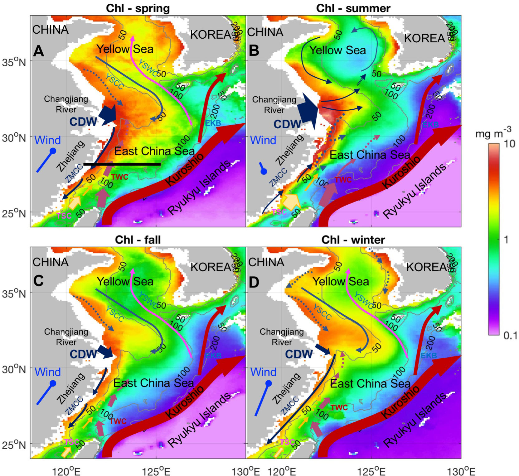
Figure 1 Satellite Chl-a seasonal climatology with sketched circulations. (A) Spring (March–May), (B) summer (June–August), (C) fall (September–November), and (D) winter (December–February). [CDW, Changjiang (Yangtze) River Diluted Water; YSCC, Yellow Sea Coastal Current; YSWC, Yellow Sea Warm Current; EKB, Eastern Kuroshio Branch; TWC, Taiwan Warm Current; ZMCC, Zhe-Min Coastal Current]. The winds illustrated are the ERA-Interim climatology of wind vectors in the 25°–30°N, 120°–127°E box, which represents the East China Sea. The gray contour lines denote the 50-, 100-, and 200-m isobaths.

The strong western boundary current, the Kuroshio Current, flows on the external edge of its broad continental shelf and transports a massive amount of warm, saline water and nutrients into the ECS shelf. The Kuroshio entering the ECS through the Taiwan Strait is considered to be the traditional route (Chen, 1996; Lee and Matsuno, 2007; Yang et al., 2018). Upwellings due to topographies along the Kuroshio path have been demonstrated as another mechanism of Kuroshio intrusion into the ECS (Lee and Chao, 2003; Wong et al., 2004; Zhou et al., 2018). Because the ECS is found to be phosphate-limited (Wong et al., 1998; Huang et al., 2019), the phosphate-rich remote Kuroshio Subsurface Water (KSSW) could play an important role in modulating nutrient fluxes and thus regulating phytoplankton bloom dynamics (Gong et al., 1997; Zhao and Guo, 2011; Liu et al., 2014). However, the Kuroshio intrusion forms a sharp sea surface temperature (SST) front, which is mostly apparent during the winter and spring when the warmer Kuroshio water meets the cold continental shelf water. The SST front can cause stronger surface winds, higher clouds, and intensified precipitation (Xie et al., 2002; Liu J. et al., 2016), which mainly occurs from spring to early summer (Sasaki and Yamada, 2018). These changes in local air–sea interactions are important for regulating local light conditions and water column stability, thus influencing phytoplankton blooms.

The ECS is influenced by large-scale coupled atmosphere–ocean variations such as the Pacific Decadal Oscillation (PDO) and El Niño–Southern Oscillation (ENSO). A broadly accepted conclusion from previous studies is that the Yellow Sea and ECS experienced a robust, persistent SST increase in the last few decades until the late 1990s (Xie et al., 2002; Oey et al., 2013; Wang et al., 2013; Pei et al., 2017), followed by significant cooling until 2014, returning to warm temperatures until now (Kim et al., 2018). These episodes reflect a phase change in the PDO. The PDO index is negatively correlated with the wind stress curl over the central North Pacific at ECS latitudes (Andres et al., 2009). When the PDO is positive, the SST is cooler and the wind stress curl is positive over a large area north of 38°N. It has also been demonstrated that the interannual variability of the Kuroshio intensity is positively correlated with the PDO index before the early 2000s (Soeyanto et al., 2014; Wu et al., 2019); however, since the early 2000s, the Kuroshio intensity in the ECS has been modulated by the combined effect of westward-migrating mesoscale eddies and westward-propagating oceanic planetary waves from the east, which results in a weak correlation between the Kuroshio intensity and PDO (Jo et al., 2022). Further studies indicated that there has been a decreasing trend of Kuroshio intrusion into the ECS during 1993–2001 and an increasing trend thereafter (Wu et al., 2017). In addition to this decadal variability, the SST in the ECS shelf has significant coherency with the Niño 3.4 SST with a phase lag of 5–9 months (Park and Oh, 2000). The mature phase of El Niño is normally accompanied by a weaker than normal winter monsoon along the East Asian coast and warmer and wetter weather than normal during winter and the following spring (Wang et al., 2000).

Although a reasonable understanding of the relationship between the physical environment and climate signals is available in the literature, the impact of climate variability on marine ecosystems is somewhat unknown, especially in terms of the phenology of phytoplankton blooms in the ECS. Meteorological forcing influences the movement of surface water via driving circulation and Ekman transport (Liu and Su, 1991); it also impacts vertical mixing through air–sea fluxes, thus causing a high possibility of bio-physical interactions in the ECS. The ECS is characterized by consistently high chlorophyll biomass [0.11–8.03 mg m⁻³, cruise data measured by fluorometers in Gong et al. (2003)] and exhibits strong seasonal cycles in biological processes (Gong et al., 2003). Satellite ocean color data have been widely used in the marginal seas of the Western Pacific to describe the response of Chl-a to environmental changes from seasonal to interannual scales (Yamaguchi et al., 2012; He et al., 2013; Liu and Wang, 2013; Liu X. et al., 2016; Kong et al., 2019; Wang et al., 2019; Yoo et al., 2019; Song et al., 2020). Phytoplankton blooms have been observed over large areas of the Yellow Sea and ECS during spring (March–April) (Kiyomoto et al., 2001; Hyun and Kim, 2003; Yamaguchi et al., 2012; He et al., 2013). An increase in Chl-a was expected when the CDW extended offshore during the summer (July–August) (Ning et al., 1998; Gong et al., 2003). In addition to seasonal variability, the ecosystems of these marginal seas are expected to respond to multiple timescales of climate-mode variability. This raises an interesting question about how the marginal sea ecosystem will respond to different modes of basin-scale environmental changes, for example, different modes of basin-scale SST variability and ENSO-regulated weather changes. Thus, a complete examination of phytoplankton phenology is necessary, considering the pivotal role of phytoplankton and their high sensitivity to marine environments (Chavez et al., 2011; Behrenfeld et al., 2016).

In this study, we re-examined the seasonal variability of Chl-a by the Empirical Orthogonal Function (EOF) analysis for 10-year SeaWiFS (Sea-Viewing Wide Field-of-view Sensor) Chl-a data (1998–2007) and 17-year MODISA (Moderate Resolution Imaging Spectroradiometer-AQUA) Chl-a data (2003–2019). Our results reproduced the dominant seasonality of Chl-a as documented in the literature. The SeaWiFS and MODISA Chl-a both showed enhanced Chl-a during spring in the Yellow Sea and ECS and summer Chl-a high in the Changjiang estuary (Figures 2A–D). Beyond this seasonality, one interesting point is that the MODISA period obtained larger Chl-a values in March and April than the SeaWiFS period (Figure 2D). Springtime is a crucial transition period during which seasonal phytoplankton blooms occur in response to monsoonal winds and changes in stratification in the ECS. The transition from winter to summer monsoon may not be consistent because climate variability modulates the weather patterns in the ECS. Therefore, the question arises as to why the most significant Chl-a increase occurs in spring, whether this increase is consistent throughout the ECS area, and how the spatial increase in Chl-a indicates the change in physical fields to some extent. To answer these questions, we attempted to provide a more holistic understanding of the interlinked physics and phytoplankton blooms in the ECS and an integrated understanding of how these mechanisms act individually and in concert to influence phytoplankton dynamics, particularly considering the impact of climate signals on this region. The independent datasets used are described in Section 2. In Section 3, when and where the interannual anomalies of Chl-a occur are investigated under the framework of coupled seasonal monsoon and climate signals that have modulated this region with remarkable physical phenomena. The mechanisms driving these fluctuations are also addressed. Our results are discussed in Section 4, and the major findings are summarized in Section 5.

FIGURE 2

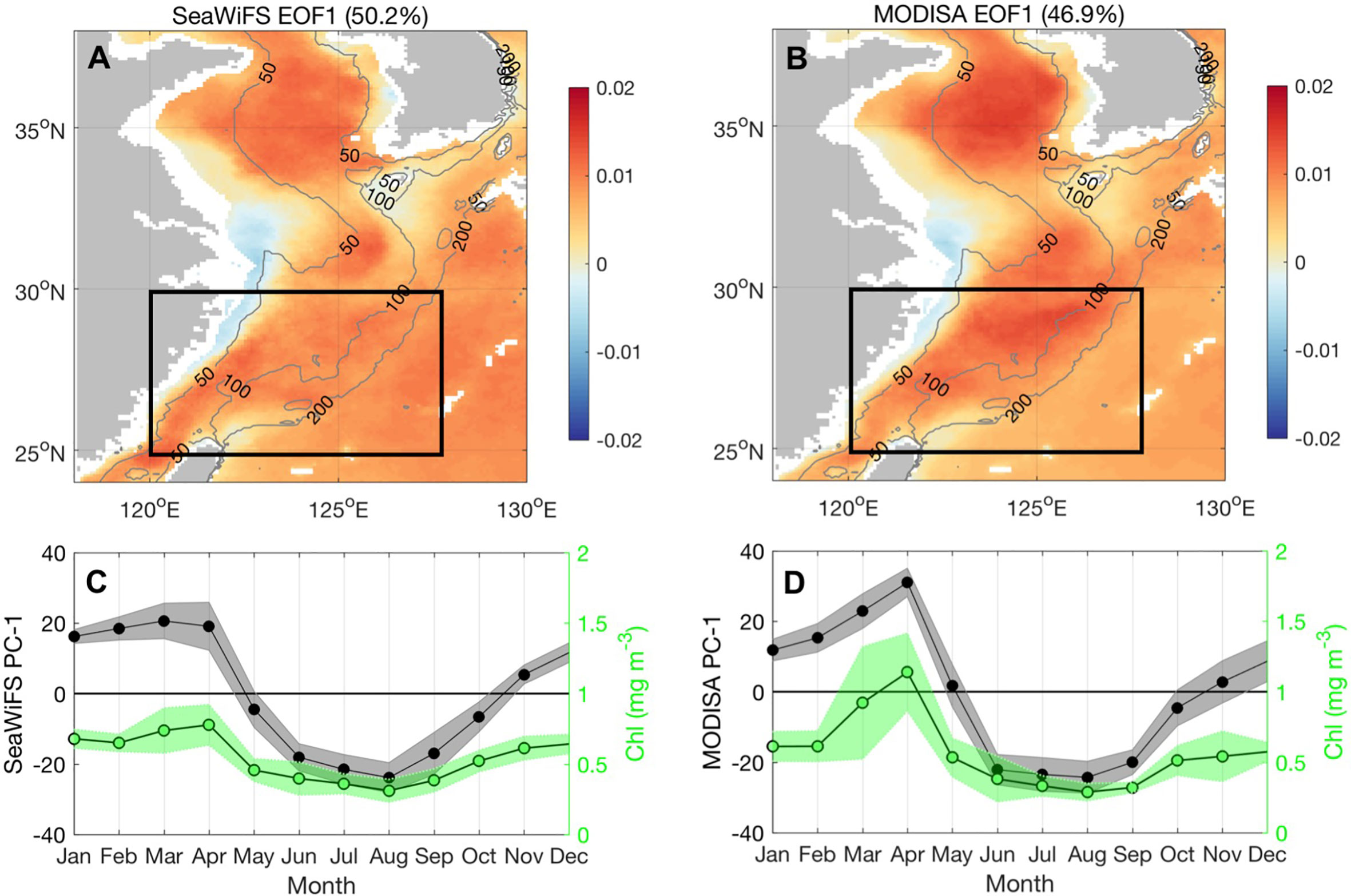
Figure 2 The EOF first mode of SeaWiFS and MODISA Chl-a. (A, B) The first EOF mode spatial coefficient of SeaWiFS and MODISA Chl-a, respectively; the gray contour lines denote the 50-, 100-, and 200-m isobaths. (C, D) The monthly averaged EOF PC-1 with standard deviations for SeaWiFS and MODISA Chl-a. The green shading in (C, D) denote the monthly climatology and standard deviations of spatial mean Chl-a in the box (25°–30°N, 120°–128°E) with water depth between 50 m and 200 m for SeaWiFS and MODISA periods, respectively.

Data and methods

Satellite remote sensing data

The time series of Chl-a in the Yellow Sea and ECS were examined using Level 3 standard mapped monthly averaged composites of 4-km-resolution SeaWiFS (based on the SeaWiFS.r2018 reprocessing results) and MODIS Aqua (based on the MODIS.r2018 reprocessing results) data collected from January 1998 to December 2007 and January 2003 to December 2019, respectively (https://oceancolor.gsfc.nasa.gov). Given the uncertainty in ocean color data to determine Chl-a variability in Case 2 optically complex waters [i.e., increasing concentrations of color dissolved organic matter (CDOM) and total suspended matter (Bowers et al., 2011)], we excluded regions with water depths shallower than 10 m for this analysis. Pixels covered by clouds were replaced by the average of eight non-cloud-neighbor pixels for each image.

We conducted a thorough analysis of time and space to compare the SeaWiFS and MODISA time series (Figure S1). The linear regression on the logarithmic scale of the SeaWiFS and MODISA overlapped period (January 2003 to December 2007) showed a significant correlation [log(MODISA_Chl_-a) = 1.02*log(SeaWiFS_Chl_-a) − 0.0354, R = 0.93, p< 0.001], which suggests that the inevitable differences between the Chl-a values retrieved by SeaWiFS and Aqua/MODIS owing to the differences in sensor performance (e.g., bands and calibration accuracy) are within the acceptable error range; thus, SeaWiFS and MODISA could be used for the continuity of Chl-a assessments. Such comparisons have been applied in regional China Seas and validated with in situ measurements, which suggest that MODISA and SeaWiFS Chl-a are very similar in their absolute values and spatial patterns (Zhang et al., 2006; He et al., 2013). This brings up the number of years with continuous Chl-a data for up to 22 years. For the first, which emphasizes temporal variabilities, EOF calculations were performed on the log of the time series, and for each time series, the overall mean of the whole time series was subtracted from each pixel. To further determine the spatial and temporal biases from different instruments, we also collected the European Space Agency’s Ocean Color-Climate Change Initiative (OC-CCI) Chl-a. The OC-CCI data were generated from merged normalized remote sensing reflectance data from multiple satellite sensors (SeaWiFS, MODISA, and medium-resolution imaging spectrometer [MERIS]). The EOF analysis based on these data indicated spatial and temporal variabilities similar to those of SeaWiFS and MODISA Chl-a (see Figure S2 in Supporting Information).

We also obtained the monthly SST based on 4-day averaged Advanced Very High-Resolution Radiometer (AVHRR) datasets from 1998 to 2019. The solar energy flux reaching the ocean surface in the spectral range of 400–700 nm, referred to as photosynthetically available radiation (PAR), controls the growth of phytoplankton, and such a time series enables examination of the role of light in phytoplankton dynamics in this region. The monthly SeaWiFS and MODISA Level 3 PAR data ranging from 1998 to 2019 were downloaded from http://oceancolor.gsfc.nasa.gov.

Model reanalysis data and observational nutrient data

Wind speed and heat flux were obtained from the ERA-Interim reanalysis product (available at https://cds.climate.copernicus.eu/cdsapp#!/dataset/), which is the global atmospheric reanalysis dataset developed by the European Center for Medium-Range Weather Forecasts (ECMWF). The local surface wind stress curl ∇×τ (,where x and y are the eastward and northward coordinates, respectively, and τ_x τ_y re the corresponding components of the wind stress) was calculated based on the monthly winds. The net heat flux (NHF) consists of four components: shortwave radiation from the sun (SW), outgoing longwave radiation (OLR) from the sea surface (LW), sensible heat transfer from air–sea temperature differences (SH), and latent heat transfer carried by evaporation (LH), with a combination of NHF = SW–LW–LH–SH. The spatial resolution of the product is 14°, and data from January 1998 to December 2019 were used in this study. When the NHF is positive, the ocean gains heat, which implies an increase in stratification, and vice versa when the NHF is negative. OLR was obtained from the latest ERA5 product (https://cds.climate.copernicus.eu/cdsapp#!/dataset/reanalysis-era5-single-levels-monthly-means?tab=overview). The OLR is a proxy for deep convection and is used as a heuristic indicator of cloudiness and associated latent heating, which, in turn, is expected to influence the amount of sunlight reaching the sea surface.

We used the outputs from a physical model based on the Regional Ocean Modeling System (ROMS) (Geng et al., 2021). The model domain covers the entire China Sea (0.0°–41.5°N, 99°–140°E), with a horizontal grid resolution approximately 9 km and 30 vertical levels in terrain-following sigma coordinates. The model was forced at the lateral open boundaries by daily temperature, salinity, and currents from the HYCOM reanalysis GLBu0.08, with a spatial resolution of 1/12° and hourly tidal elevations calculated from eight tidal constituents (M2, S2, N2, K2, K1, O1, P1, and Q1). The model was driven by 6-hourly reanalysis atmospheric forcing data provided by the NCEP/NCAR. The model includes 26 major rivers. The model was integrated between the years 2000 and 2015. Extensive validation of the model revealed that it reproduces the observed patterns of the upper ocean structure of marginal Chinese seas (Geng et al., 2021). We used outputs from 2011 to examine the oceanic fields this year because of the strong 2010/11 La Niña concurrent in the negative PDO phase, which provides an opportunity to gain a better understanding of climate anomaly induced phytoplankton variability.

Climatological values of 1° resolution WOA18 (Boyer et al., 2018) nitrate data were used for nitracline estimation. The bottom of the nitrate-depleted surface layer (referred to in the following as the “nitracline”) was defined as the depth where the nitrate concentration exceeds 0.5 µM (https://www.ncei.noaa.gov/data/oceans/woa/WOA18/DATA/). A 0.25° resolution mixed layer depth (MLD) was obtained from https://www.ncei.noaa.gov/data/oceans/woa/WOA18/DATA/.

We attempted to monitor ENSO by using the multivariate ENSO index (MEI; https://psl.noaa.gov/enso/mei/), which is the time series of the leading combined EOF of six different variables (sea level pressure, SST, zonal and meridional components of the surface wind, and OLR) over the tropical Pacific basin (30°S–30°N and 100°E–70°W). The PDO is defined as the leading EOF of SST anomalies north of 20°N in the Pacific Ocean and is often described as a long-lived El Niño-like pattern of Pacific climate variability (Mantua et al., 1997; Zhang et al., 1997). When PDO is positive, the (anomalous) SST is cooler over a large area north of 38°N, but SST is warmer off the northwestern coast of North America as well as in the central Pacific from 20°N to 38°N. Updated monthly data are available at http://jisao.washington.edu/pdo/.

Results

Seasonal pattern of physical fields

To interpret the possible physical factors influencing Chl-a variability, the most dominant seasonal distribution of the physical fields (including SST, PAR, wind stress magnitude, and NHF) was investigated using the EOF analysis method (Figure 3). First, we focused on investigating how different factors could be related to the seasonal dynamics of Chl-a, including its spatial distribution and temporal variability.

FIGURE 3

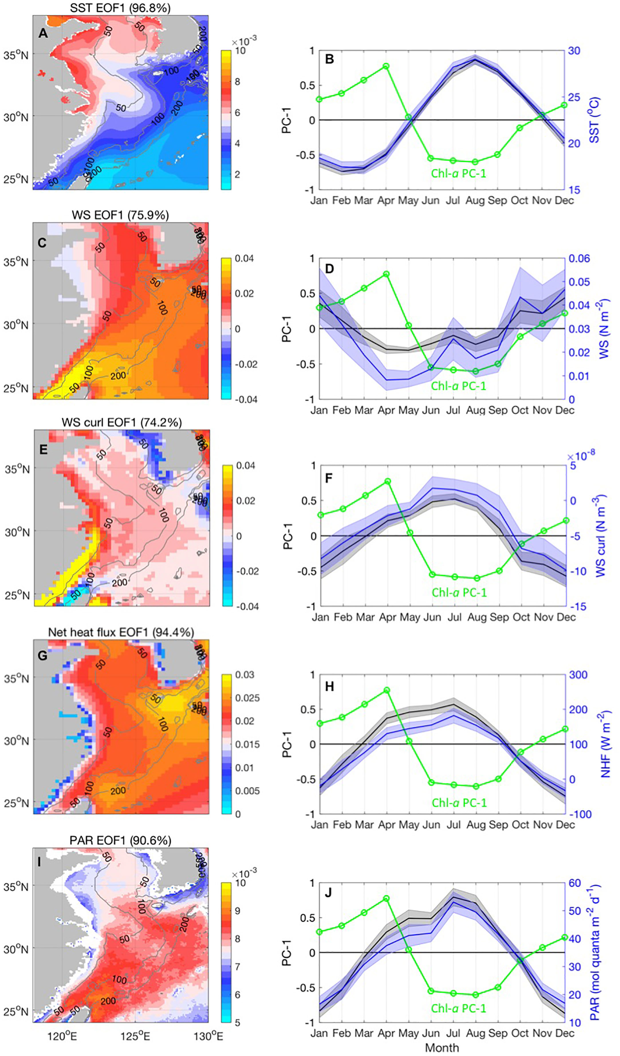
Figure 3 The first EOF mode eigenvectors and monthly averaged temporal amplitude (PC) for SST(A, B), wind stress magnitude (C, D), wind stress curl (E, F), NHF(G, H), and PAR (I, J). The averaged value of these variables in the box of Figure 2 was overlaid on the monthly PC time series. The monthly averaged normalized MODISA Chl-a PC-1 was plotted as a green line in each PC of the environmental variables.

The first EOF mode of SST (Figure 3A) explained 96.8% of the total variance. This is related to the seasonal increase in SST, starting in March and reaching a maximum in August (Figure 3B). All spatial coefficients are positive, with the maximum value found nearshore in the Yellow Sea, which suggests more significant seasonal temperature variability in these areas. The Kuroshio Current leaves a northeast-directing warm tongue in the SST field between the continental shelf and the Ryukyu Islands, forming a sharp SST front. The magnitude of the SST variability over the continental shelf is larger than that over Kuroshio. This difference is probably because the heat content that is roughly proportional to the bottom depth of the water column is smaller over the continental shelf than that in the Kuroshio axis region (Xie et al., 2002). The spatial pattern of wind stress was clearly associated with SST. This indicates consistent signs throughout the area, with high values situated over the Taiwan Strait due to the orographic effect over land and extending northeast over the pathway of the Kuroshio Current (Figure 3C). Near the Kuroshio SST front, the surface air temperature is not in equilibrium with SST, especially in winter, which results in an unstable atmosphere on the warmer flank of the front with strong turbulent mixing that conveys stronger winds from aloft, accelerating the surface wind. The corresponding temporal evolution is characterized by strong seasonal cycles with peaks in December and troughs in May (Figure 3D). The positive phase lasted from October to February of the following year, suggesting a more surface wind mixing condition. During winter, extensive northeasterly/northwesterly winds prevail over the ECS shelf with increased magnitude offshore from the coast to the 100-m isobath, which results in a negative wind stress curl over the inshore area and a positive wind stress curl east of the 100-m isobath (Figures 3E, F). The variability was most significant over the Taiwan Strait owing to the tunnel effect. During summer, a positive wind stress curl is imposed west of the 100-m isobath inshore area, which is maximized over the coast of Zhejiang and Fujian.

The EOF of the NHF indicated the maximum spatial variability over the Kuroshio and strong heat loss in winter from October to February (Figures 3G, H). PAR also indicated high spatial variances northeast of the pathway of the Kuroshio Current. Its values peaked in July and were lowest in December–January. Because clouds reflect incoming shortwave radiation back into space, the change in cloudiness is directly associated with the change in the PAR signal. A lower (higher) cloud amount or albedo translates into a higher (lower) PAR, making the atmosphere less reflective. In this region, Xie et al. (2002) reported increased cloudiness over the warm tongue on the warmer flank of the Kuroshio SST front in the winter season, which corresponds with the PAR seasonality in this analysis. These in-phase relationships between SST, surface wind, NHF, and PAR are indicative of the strong seasonality of air–sea interactions in the Kuroshio area (Zhang and Li, 2020).

Our analysis above indicates that the phase changes of the physical fields are concentrated around March, when the traditional spring phytoplankton bloom occurs in the central Yellow Sea and the ECS shelf. Phytoplankton blooms occur only after solar radiation begins to increase, which increases the flux of light to the surface ocean and helps stabilize the water column by warming the surface water. This allows the cells to overcome chronic light limitation in a deeply mixed water column. In our analysis, the initiation of the spring bloom was phased around one month after the onset of SST warming in the southern ECS (Figure 3A). This is consistent with the hypothesis that blooms begin as the water column stratifies as a result of increased PAR, decreased wind stress, and NHF turning from negative to positive. Thermal stratification develops as the frequency of winter mixing decreases, and the surface ocean becomes heated, both of which induce phytoplankton blooms in the spring in the shallow surface-mixed layer. The bloom disappeared in summer, and strong stratification developed. This Chl-a seasonality is consistent with the classical spring bloom in temperate shelf regions (Sverdrup, 1953), which coincides with the onset of thermal stratification, although the winter conditions are not as extreme as at high latitudes.

Interannual variability of Chl-a

Considering that phytoplankton seasonality is determined by variations in the physical environment, it can be reasonably assumed that interannual variations in physics also alter Chl-a. Understanding how phytoplankton will respond to climate change is especially important, as the ECS has experienced significant changes in water properties over the last few decades, and a 22-year time series of consistent Chl-a could provide a measure of the biological state of the surface ocean to such environmental changes over long periods.

The Chl-a spatial distribution and associated magnitude of variance were individually examined for the SeaWiFS and MODISA periods. The overall spatial distributions of Chl-a determined using the SeaWiFS and MODISA data were similar, with gradual decreases from the coastal region to the shelf (Figures 4A, C). There were high standard deviations of Chl-a in the coastal area, especially in the Changjiang River estuary, which could be associated with riverine inputs (Figures 4B, D). The high standard deviations in the central Yellow Sea waters are due to local winds, air–sea fluxes, and tidal mixing (Guan, 1994), which lead to an ~30% amplitude of changes (Figures 4B, D). Compared with the coastal waters and the sea adjacent to large river mouths, the offshore southern ECS shelf waters between 50 and 200 m have relatively lower averaged Chl-a (~0.5 mg m⁻³), but display large dynamic range (STD can be as high as ~0.5 mg m⁻³, ~100% amplitude of changes). This suggests significant interannual variability in biology due to the background of the more complex hydrodynamics in this region. To avoid directly comparing and merging the SeaWiFS and MODISA Chl-a data, which are based on different sensors, separate EOF analyses were performed for the SeaWiFS and MODISA Chl-a time series to compress the spatial and temporal variability of each time series into a set of dominant modes with spatial functions and associated time-varying amplitudes. To reduce the effects of strong seasonal signals in the time series, EOF analysis was applied to the Chl-a anomalies in which the seasonal cycle was removed by subtracting the monthly climatology. Such a time series provides a means of investigating the interannual variability of oceanic primary production.

FIGURE 4

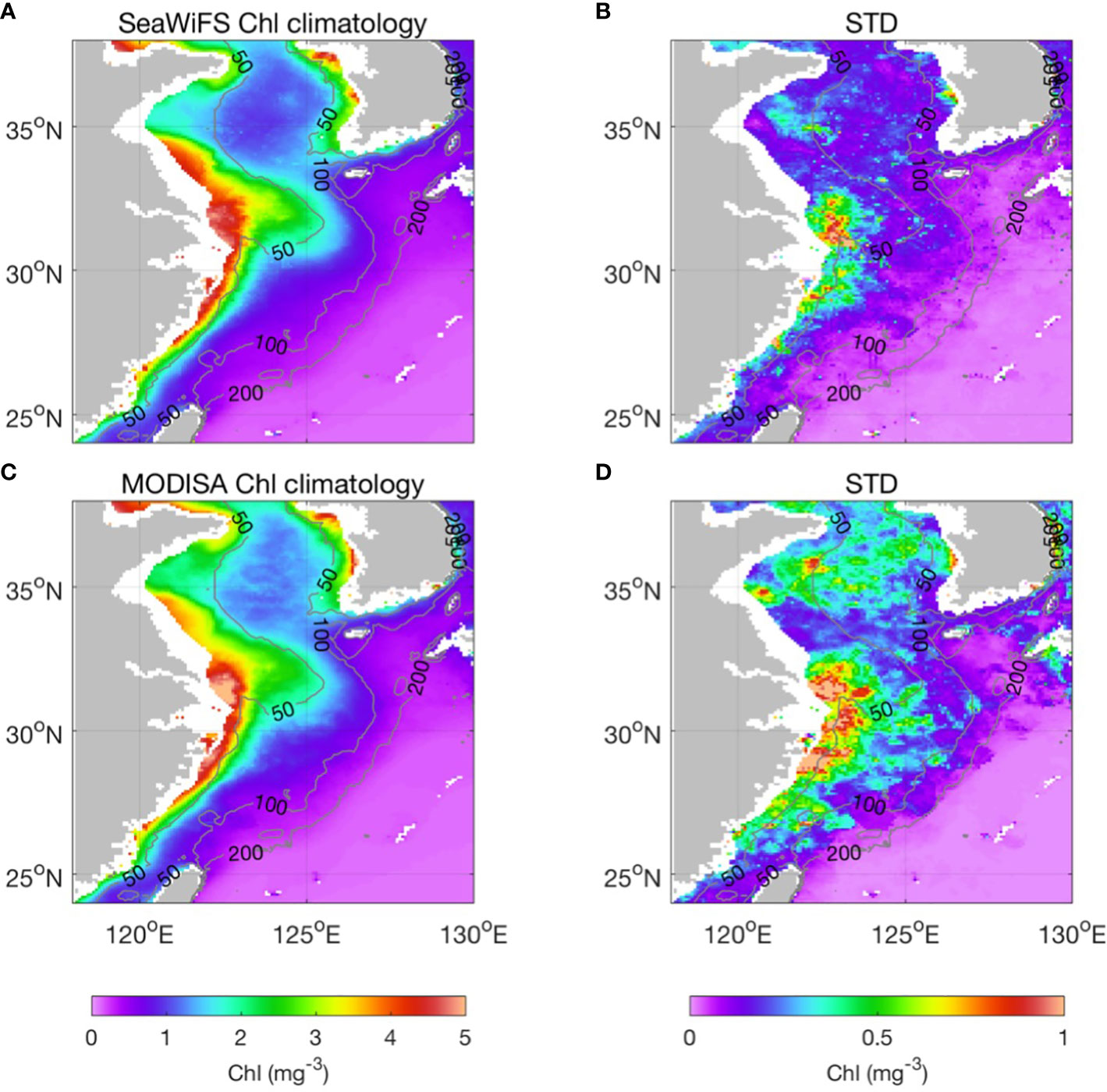
Figure 4 Climatology distributions of the mean (left column) and standard deviation (right column) of Chl-a for SeaWiFS (1998–2007, upper panel A, B) and MODISA (2003–2019, bottom panel C, D). The gray contour lines in each map denote the 50-, 100-, and 200-m isobaths.

The eigenvectors of EOF analysis of the SeaWiFS and MODISA Chl-a anomaly fields identify a similar spatial pattern in that significant variance occurs in a triangular area located in the mid-shelf south of the 32°N ECS, between the 50- and 100-m isobath (Figures 5A, B). This triangular area reminded us of the position of the three fronts in the ECS (Belkin et al., 2009; Chen, 2009; Huang et al., 2010; Liu et al., 2018): the Zhejiang-Fujian front, which is the boundary between the TWC and the ECS coastal current, formed along the 50-m isobath, the Yangtze Bank Ring front surrounds the Yangtze Bank (Shoal) caused by the huge fresh discharge of the Changjiang River, and the Kuroshio SST front. Time series of Chl-a averaged for the region (123–125°E, 28–30°N box) where the EOF spatial coefficients are larger than 0.015 (Figure 5D) indicates a similar temporal variability to that of EOF PC-1 (Figure 5C), which both indicated significant interannual variabilities. The monthly climatology of Chl-a indicated that interannual departures mainly occurred in spring (March and April) (Figures 2C, D). Although the dynamics and patterns of seasonal spring phytoplankton blooms are well founded in this region, less is known about what accounts for the remarkable interannual variability in this area, which stands out elsewhere in the Yellow Sea and ECS.

FIGURE 5

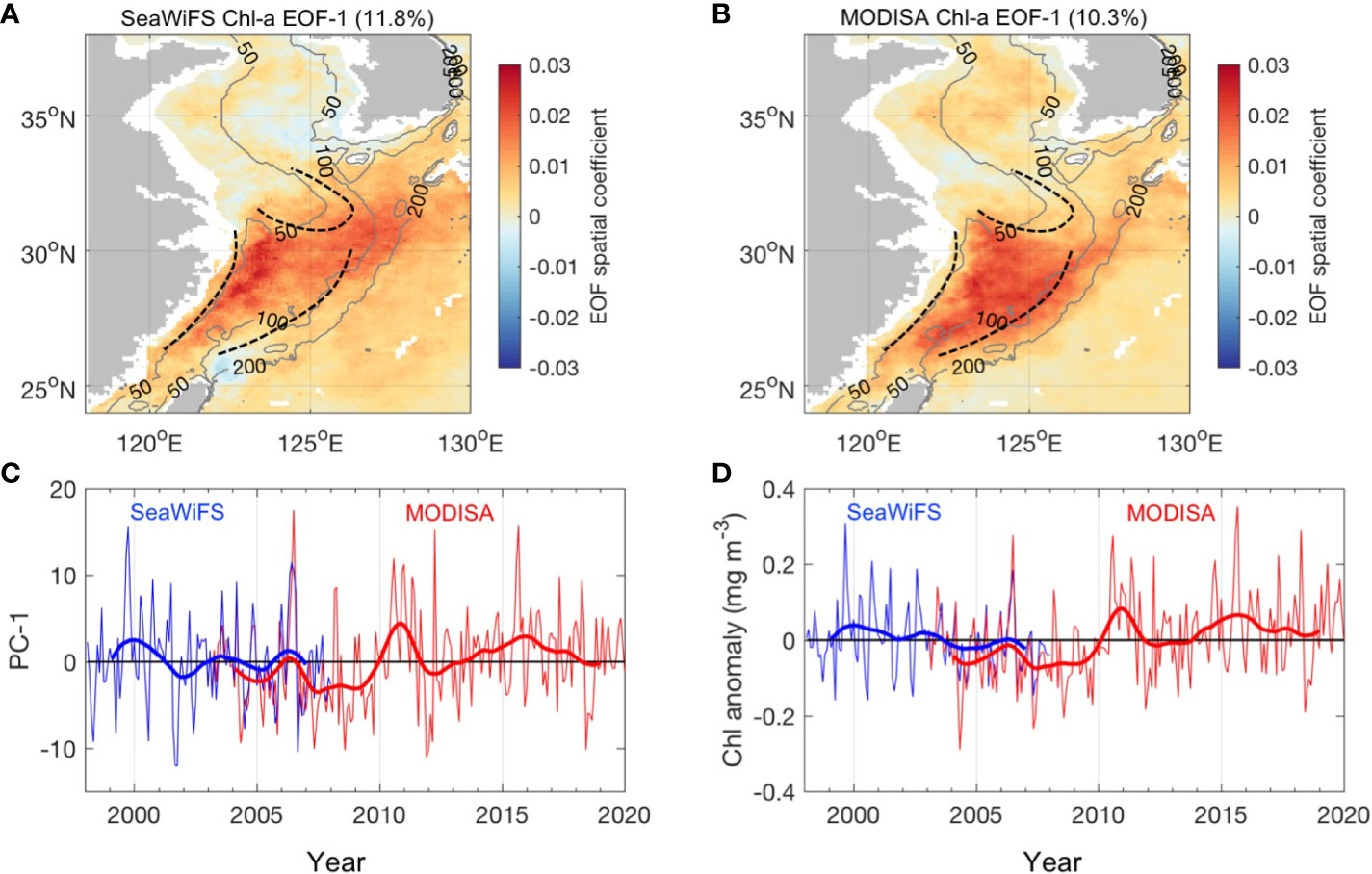
Figure 5 EOF analysis of Chl-a anomalies. (A, B) The spatial coefficient of the first EOF mode for the SeaWiFS and MODISA Chl-a anomalies, respectively; the black dashed contours indicate the position of the fronts referred from Belkin et al. (2009) and Liu et al. (2018). The gray contour lines in each map denote the 50-, 100-, and 200-m isobaths. (C) The EOF temporal amplitude (PC) for SeaWiFS (blue) and MODISA (red) Chl-a. The thick blue and red lines denote the 12-month low-pass-filtered PC-1. (D) Time series of Chl-a anomalies averaged for the area in the mid-shelf of ECS where the EOF eigenvectors are larger than 0.015.

Dynamical factors contributed to the interannual variability of Chl-a

To investigate the possible driving factors for the significant Chl-a interannual anomaly occurring in the mid-shelf ECS, the concurrent local environmental disturbances over the ECS during these 22 years were further quantified in this subsection including wind stress, wind stress curl, NHF, SST, and PAR.

The ECS spring bloom is promoted by a transition from deep convection to a shallow mixing layer concurrent with increasing light intensities in nutrient-enriched waters; thus, winds can influence the structure of the water column and, thereby, the timing and magnitude of the spring bloom. Therefore, interannual variability in bloom magnitude will occur through variability in winter and spring mixing conditions. Winter mixing also determines the nutrient concentration in the euphotic zone, which is available for new production the following spring. An EOF examination of the northerly wind stress anomalies over the ECS indicated the largest spatial variability in the northeast of Taiwan Island (Figure 6A), which is the same region with the most significant interannual variability of Chl-a (Figures 5A, B). The EOF PC-1 of northerly wind anomalies generally indicates a negative correlation with Chl-a PC-1, with a relatively weak correlation (r = −0.28, p< 0.001); the correlation coefficient was the mean of the SeaWiFS and MODISA periods). This is due to the opposite correlation between wind and Chl-a along the time series. There were two periods (2000 and 2011) in which the most pronounced positive Chl-a PC-1 corresponded to positive wind PC-1. Combined with the negative EOF spatial coefficient (Figure 6A), this suggests that there is a strengthening of northerly winds (positive wind PC-1) accompanied by anomalously high Chl-a in the southern ECS. In contrast, there was a period (e.g., after 2015) in which there was a weakening of northerly winds and anomalously high Chl-a.

FIGURE 6

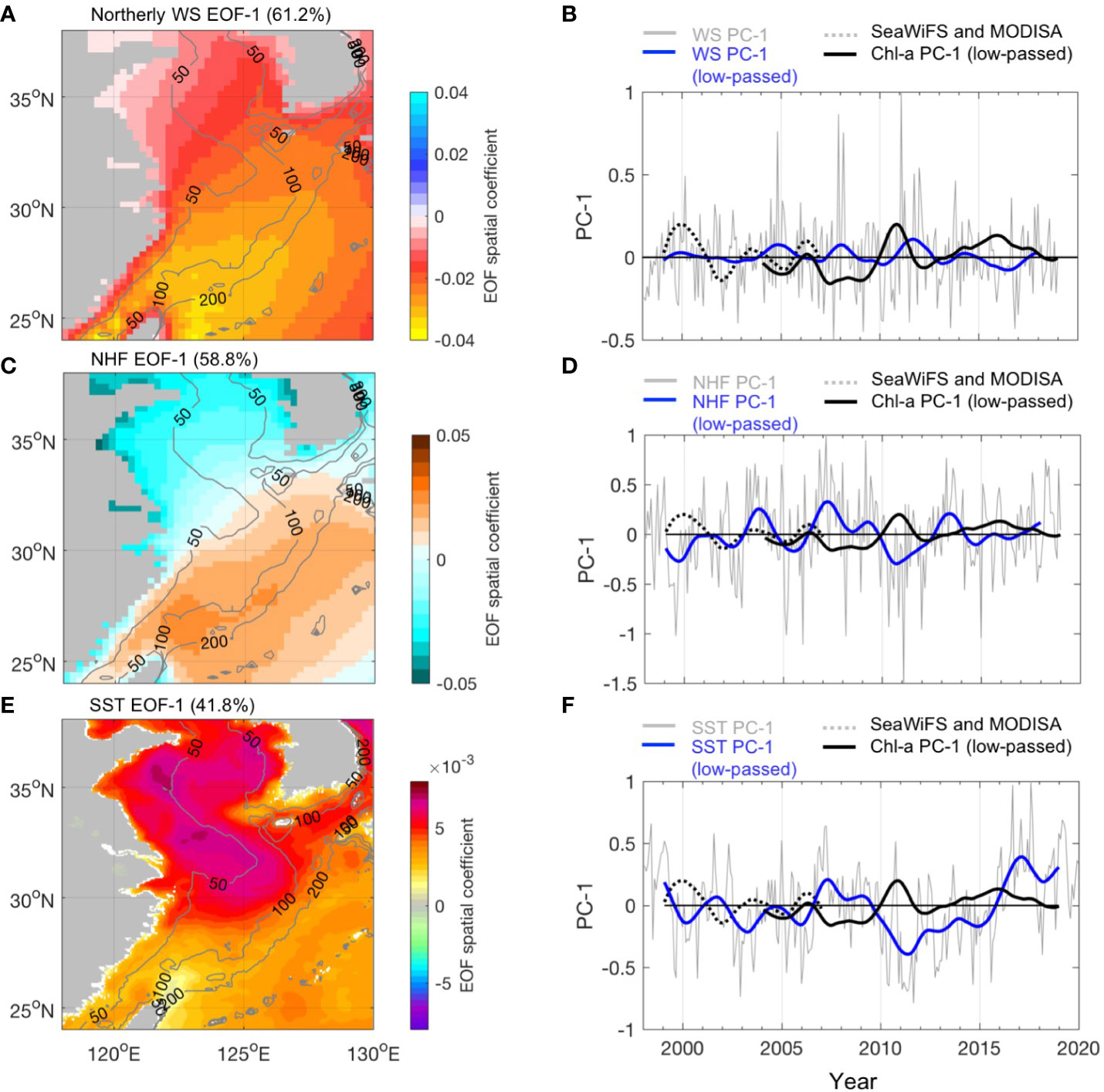
Figure 6 The first EOF mode for northerly wind, SST, and NHF. (Left) The EOF spatial coefficient. The gray contour lines in each map denote the 50-, 100-, and 200-m isobaths. (Right) (Left A, C, E) the EOF spatial coefficient. The black dashed and thick lines in (B–F) indicate the 12-month low-pass-filtered PC-1 for SeaWiFS and MODISA Chl-a, respectively.

The heat flux is also a major force for water column stability because it regulates stratification during the spring transition season, thus influencing the Chl-a variability (Figures 6C, D). The first EOF mode presents the maximum NHF variability over the Kuroshio between 100 and 200 m, which is consistent with the high-variability region identified by the EOF of wind stress. This high variability could be associated with the Kuroshio SST front because, over the front, the surface air temperature is not in equilibrium with SST, which results in an unstable atmosphere on the warmer flank of the front and strong turbulent mixing that conveys stronger winds from the aloft and accelerates the surface wind (r = −0.51, p< 0.001).

The EOF mode 1 for SST indicates coherent positive spatial coefficients in the Yellow Sea and ECS, with the maximum variability centered east of the Changjiang River mouth and the south of Shandong Peninsula (Figure 6E, dark red, with EOF eigenvectors as large as 0.008) and relatively low magnitude of variability in the southern ECS (Figure 6E). This result is quite similar to the leading EOF mode 1 estimated based on the NOAA/AVHRR SST for the periods 1981–2009 (Park et al., 2015) and 1982–2014 (Kim et al., 2018), respectively. It appears that the largest anomalies in Chl-a were not at the exact locations where the largest SST anomalies occurred. One possible reason for this inconsistency could be that the most significant changes in Chl-a are over regions (the triangular area in Figures 5A, B), where the mean Chl-a values are relatively small (Figure 1) while the SST is high. Thus, the correlation between SST PC-1 and Chl-a PC-1 was relatively weak (r = −0.25, p< 0.001).

The EOF of the PAR spatial maps and the associated amplitude time series derived from the SeaWiFS and MODISA time series are displayed in Figure 7. The spatial pattern of EOF mode 1 (31.9% and 33.9% of the total variance for SeaWiFS and MODISA PAR, respectively) clearly illustrates a positive coefficient over the entire study area and relatively large variability over the southern ECS between the 50- and 100-m isobath, which is the same area identified by Chl-a EOF mode 1. EOF mode 1 of OLR indicates a spatial pattern similar to that of PAR (Figures 7A, B red contour lines), and a very close correlation between PAR PC-1 and OLR PC-1 (r = −0.99, p< 0.001). This suggests that when the triangular area has intense convection (e.g., when OLR PC-1 is positive), there are more clouds, thus decreasing PAR values. The corresponding PC-1 suggests a strong negative correlation with Chl-a EOF PC-1 (r = −0.52, p< 0.001). The effects of PAR on Chl-a could be non-linear; it could have a positive influence on Chl-a within a window of optimum light conditions for phytoplankton growth, and a negative impact for higher or lower PAR levels; thus, any PAR anomalies could induce significant variance in Chl-a due to photo-physiological mechanisms in phytoplankton cells. The MODISA-derived climatological euphotic zone depth (Z_eu) shows a strong coastal-offshore gradient, ranging from 40 to 70 m for the 50–200 m isobath domain (Shang et al., 2011). This suggests that a significant fraction of the water column on the shelf resides above the euphotic zone; thus, the ECS shelf is rarely light limited. From another perspective, the PAR value is directly affected by cloud coverage, which is associated with local weather conditions. Thus, the strong correlation between PAR and Chl-a may indirectly reflect the influence of weather conditions on Chl-a.

FIGURE 7

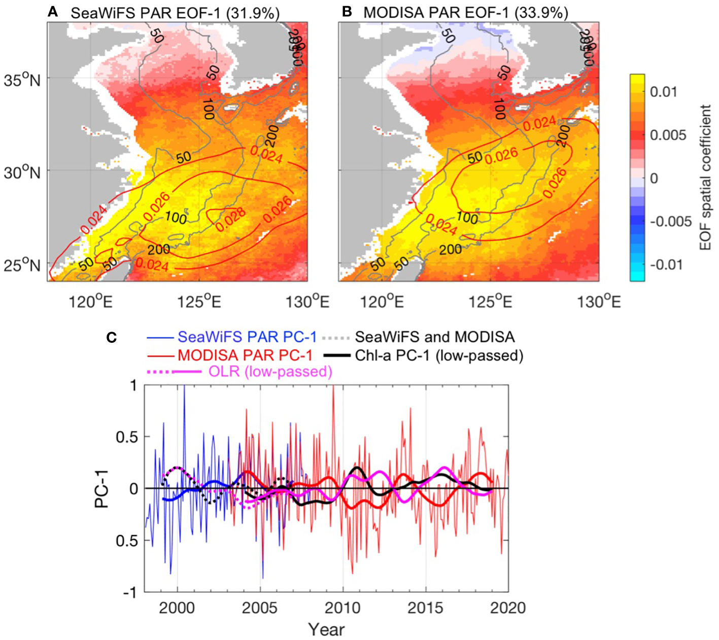
Figure 7 (A, B) Spatial coefficients of the first EOF mode for the SeaWiFS and MODISA anomalous Chl-a and OLR fields, respectively. The overlapped red contour lines denote the eigenvector of the first EOF mode of the OLR, which explains 49.7% and 52.3% of the total variance in the SeaWiFS and MODISA periods, respectively. The gray contour lines in each map denote the 50-, 100-, and 200-m isobaths. (C) Normalized EOF temporal amplitude (PC) for the SeaWiFS (blue) and MODISA (red) PAR. The thick blue and red lines denote 12-month low-pass PC-1. The black dashed and thick lines indicate the 12-month low-pass PC-1 for Chl-a during the SeaWiFS and MODISA periods, respectively. The pink lines indicate the low-pass PC-1 for OLR during the SeaWiFS and MODISA periods, respectively.

Based on the above analysis, we found that the interannual variability of Chl-a is correlated with weather conditions; however, these factors are intrinsically related. Previous studies reported the influence of large-scale modes of atmospheric variability on the physical fields of the ECS (Liu et al., 2019). In the present study, we focused on the influence of climatic forcing on Chl-a and physical factors in the triangular area of the southern ECS identified by the EOF analysis in the early part. We restricted our analysis to PDO and ENSO because they are widely used indices for which there are well-known mechanistic explanations in the ECS (Qiu, 2002; Han and Huang, 2008). The correlation coefficients between the low-pass EOF PC-1s of physical factors and Chl-a with PDO and ENSO indices are shown in Table 1. The visual coherence between the PDO and ENSO indices was high (Figure 8A). This indicates similar correlations between PDO/ENSO and Chl-a (Figure 8A), yielding a modest positive correlation between both (R = 0.28 and 0.31, respectively). This is associated with the in-phase variabilities of Chl-a and PDO/ENSO, especially after 2014, when both PDO and ENSO entered a positive phase (Figure 8A), whereas significant negative correlations were observed in two La Niña events (1999–2000 and 2010–2011). There are high correlations between the PDO/ENSO and wind terms and relatively low correlations with SST and NHF. There was no significant correlation between PDO/ENSO and PAR PC-1. This is probably because of the complicated relationship between ENSO and Madden–Julian oscillation (MJO), for which the influence of ENSO on precipitation in East Asia is different depending on the location of MJO (Chen et al., 2020). Since relatively long data records are needed to define and understand the PDO, we used the MEI index to analyze the influence of climate variability on the Chl-a and wind fields in the whole study area during the period 1998–2020. The MEI was negatively correlated with Chl-a in most of the Kuroshio water area, where the correlations exceeded –0.8. It is positively correlated with Chl-a in much of the ECS, especially in the triangular area identified by Chl-a EOF mode 1 (Figure 8B), and can be as large as 0.6. The correlations between the wind and MEI were more consistent over the ECS. The area of negative correlation between wind stress and MEI (Figure 8C) and the positive correlation between northerly wind and MEI (Figure 8D) extend from the Kuroshio area to the north, resulting in an area with the most significant correlation between MEI and wind field in the triangular area.

TABLE 1

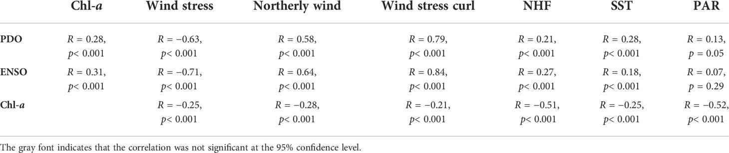
Table 1 Correlation coefficients between the EOF PC-1 of physical variables and Chl-a concentration with PDO and ENSO indexes.

FIGURE 8

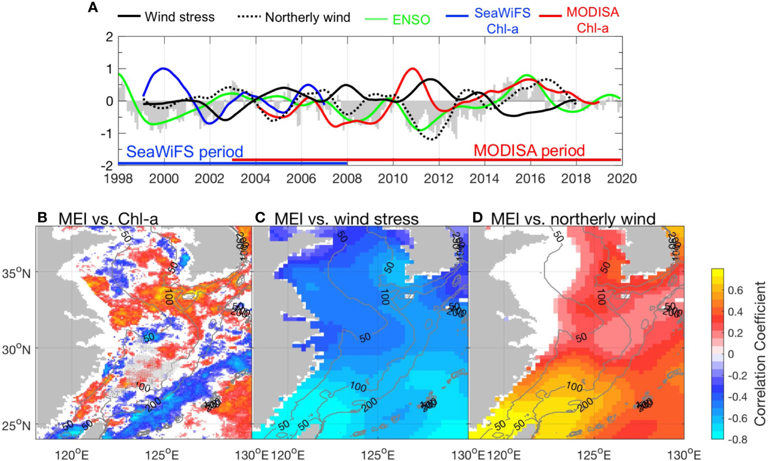
Figure 8 (A) The time series of the 12-month low-pass normalized EOF PC-1 for SeaWiFS (blue), MODISA (red) Chl-a, wind (solid black), northerly wind (dashed black), and MEI index (green). The gray bars denote the PDO index. (B) The correlation coefficient between MEI and Chl-a during 1998–2020. The area detected by EOF mode 1 with significant Chl-a anomalies is marked with a + sign. (C) The correlation coefficient between MEI and wind stress during 1998–2020. (D) The correlation coefficient between MEI and northerly wind during 1998–2020. All the correlation coefficients shown here surpassed the 95% significance level. The gray contour lines in each map denote the 50-, 100-, and 200-m isobath.

During the period of satellite Chl-a data in this study, the low-frequency PDO index entered a positive phase around 2015 from a negative phase (1999–2014). During this recent positive phase, there are decreases in wind stress and north wind, continuous SST increases, and a gradual increase in surface heating (Figure 9), which are characteristic conditions in positive PDO and ENSO modes (Qiu, 2002; Han and Huang, 2008; Nakamura, 2020). These temperate pre-spring and spring conditions resulted in significant Chl-a increases, and the highest Chl-a level was found in 2018 (Figure 9, green lines). This is consistent with the stratification control hypothesis, which states that stable stratification contributes to phytoplankton blooms.

FIGURE 9

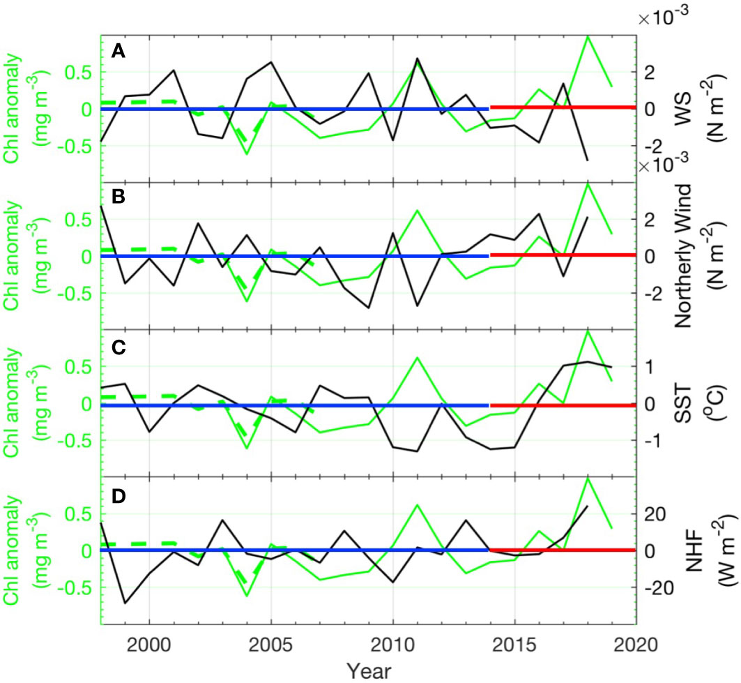
Figure 9 Time series of the spring time spatial mean Chl-a in the triangular area (Figure 8B marked with +) with (A) wind stress anomaly, (B) northerly wind stress anomaly, (C) SST anomaly, and (D) NHF anomaly. The dashed green line denotes the SeaWiFS Chl-a and the green line denotes the MODISA Chl-a. The blue straight line denotes the negative PDO period, and the red straight line denotes the positive PDO period.

The positive correlation between the MEI and Chl-a reveals that there should be a decrease in Chl-a in the negative PDO/ENSO mode. However, in our analysis, high Chl-a levels were found during the negative PDO and ENSO phases (1999–2000 and 2010–2011), when there were stronger northerly winds. Many studies have proven that La Niña is usually accompanied by a stronger than normal winter monsoon along the East Asian coast, and consequently a colder and drier winter and pre-spring (Chen et al., 2000; Wang et al., 2008). In our analysis, the 2011 spring (La Niña mode) experienced one of the lowest SST (Figure 9C) and strongest wind mixing along the time series, which is mostly associated with the enhanced northerly wind (Figures 9A, B); however, there was a significant Chl-a increase (Figure 9, green line). This seemingly brings the fundamental assumption in the stratification control model for spring phytoplankton bloom into question, indicating that the links between upper layer stratification, wind mixing, SST changes, and biological responses are more complex than the simple paradigm that sequentially relates stronger stratification with warmer SST and an enhancement of the phytoplankton population in this region.

Discussion

Based on 22-year satellite Chl-a data, we found that while the southern ECS is characterized by low Chl-a concentration, the most significant interannual Chl-a anomalies occurred in spring in a triangular area in the southern ECS. This area is surrounded by three fronts and has experienced pronounced interannual anomalies in atmospheric forcing. Positive Chl-a anomalies in this area occurred under both favorable and unfavorable stratification situations. The development of phytoplankton blooms under unfavorable stratification conditions with higher wind mixing and lower SST in spring brings the fundamental assumption of the stratification control model for spring blooms into question. We link this mixing of favorable phytoplankton bloom with the unique hydrodynamical structure due to the influence of climate signals (i.e., PDO and ENSO) on the marine environment in this area. This physical–biological coupling between the climate cycle and ecosystem dynamics is a consequence of altered nutrient flux pathways resulting from changes in stratification and circulation.

A seasonal diary of phytoplankton bloom dynamics in the ECS

Following the classic description of the conditions necessary for phytoplankton blooms, several physical factors are known to impact bloom timing or productivity, primarily local light, wind mixing, and stratification (Sverdrup, 1953). Seasonal stratification is well-characterized by the potential energy anomaly (PEA) calculated based on the density field. The PEA provides a measure of stratification that is appropriate for both coastal and shelf seas (Xu et al., 2020). Here, we examined the PEA along 28°N across the triangular area in 2011, since anomalously high Chl-a occurred when there was stronger wind and anomalously low SST in the spring of 2011. The shallow coast is well mixed throughout the year (PEA is close to zero), with an alongshore downward coastal current year, except in summer, which is referred to as the ZMCC (Figure 10A, contour lines). The mid-shelf remains well mixed from January to February, followed by a substantial increase in stratification in April (Figure 10A). The mean velocity in the mid-shelf is characterized by northeast currents, which denote the TWC. This is also reflected by a wider spread cross-shelf component during spring, when there is increased stratification and Chl-a concentration (Figure 10B). This reminds us that overall productivity may be enhanced by this circulation-associated water mass, which is partially responsible for setting stratification or nutrient levels. In these cases, blooms can occur in the presence of new nutrient sources. Most of this occurs when nutrients at the surface are already used up by phytoplankton. At this time, any process that transports nutrients to the surface mixed layer could trigger a bloom and lead to a substantial Chl-a anomaly. This could be due to gusty wind mixing, wind divergence-induced pumping, cross-shore transport, or remote nutrients brought by circulations.

FIGURE 10

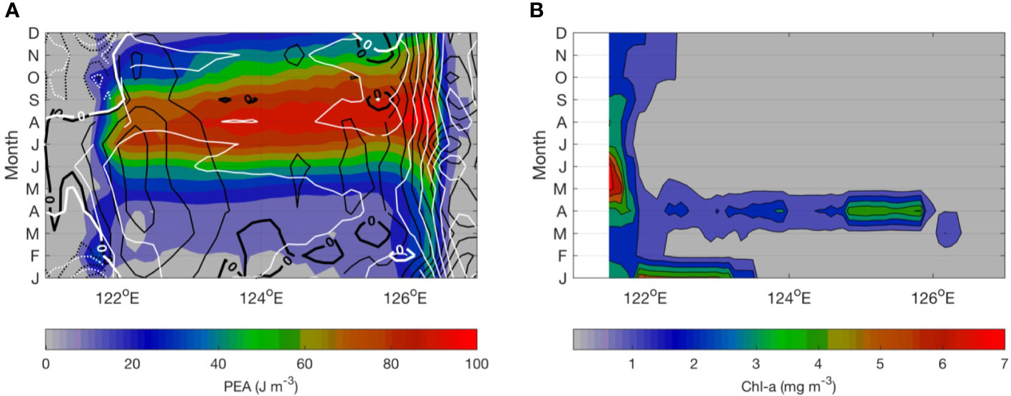
Figure 10 (A) Monthly variability of potential energy anomaly (PEA) with integration limited from surface to 200 m along the 28°N section based on model output in 2011. The PEA is zero for a fully mixed water column, positive for stable stratification, and negative for unstable stratification. The black contour lines indicate the depth-averaged north–south currents, with northward denoting positive values (black solid lines) and southward denoting negative values (black dashed lines). The white contour lines indicate the east–west currents, with eastward denoting positive values (white solid lines) and westward denoting negative values (white dashed lines). (B) Monthly variability of MODISA Chl-a along the 28°N section in 2011.

The water mass and nutrient conditions along the 28°N section were explored further. For the mid-shelf ECS, one possibility could be the influence of the TWC. The TWC, which is a mixture of the Taiwan Strait water and Kuroshio intrusion water, has been suggested to have an important impact on the hydrographical conditions and nutrients in the western ECS shelf area in many previous studies (Chen, 1996; Zhang et al., 2007; Liu et al., 2014; Zhang et al., 2019). The TWC initially flows in a northeastward direction but turns eastward around 28°N, 123°E, and further flows eastward to 125°E (Guo et al., 2006). This northeast transportation can be clearly observed in our modeled current field (Figure 10A, contour lines). The proportion of Taiwan Strait water and Kuroshio intrusion water changes with season, which means that the nutrient composition also changes when the TWC arrives at the ECS.

The vertical distributions of the WOA climatology of temperature, salinity, and nitrate along the 28°N cross-shore section were selected to represent the pre-spring (March) and spring (April) stratification and nutrient conditions (Figure 11). The dashed lines denote the depth of the euphotic layer, and the black lines denote the mixed layer depth. Based on the temperature and salinity properties and information from the literature (Zhang et al., 2007; Zhang et al., 2019), we separated the different water masses in this section. In March, the coastal region (<50 m depth) was well-mixed. The nitrate concentration was relatively high in a narrow area within the 50-m isobath. The mixed layer depth is lower than the euphotic zone from the coast to 124°E, which suggests that the majority of the water column is light-limited in the inter- and mid-shelf, whereas nutrient limitation is low. The broad ECS shelf is thus dominated by high-salinity TWC water (Figure 11C), which has a high proportion of Kuroshio incursion water from the east of Taiwan (Tang et al., 2000; Hsin et al., 2013). This water mass has a nitrate concentration of approximately 2 μ l/kg, which provides the basis of nutrients for the spring bloom; thus, the nutrient levels that persist throughout the winter could influence the magnitude of the phytoplankton bloom in the coming spring.

FIGURE 11

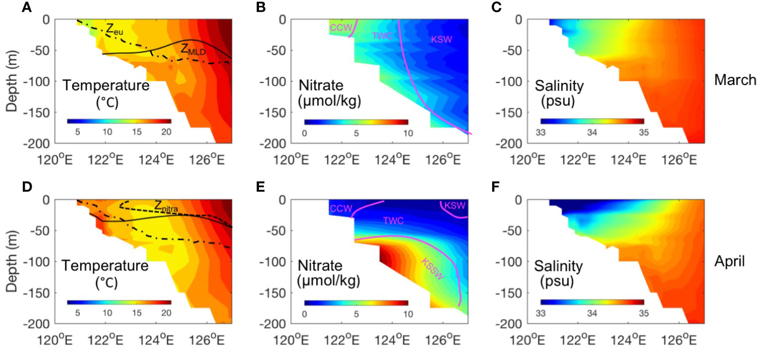
Figure 11 WOA18 climatology distributions of temperature(A, D), nitrate(B, E), and salinity (C, F) at the 28°N section. The black line denotes the mixed layer depth. The black dashed line denotes the nitracline depth (nitrate concentration exceeds 0.5 mmol/kg).

In April, seasonal stratification started to develop and mixed layer shallows. A nitracline formed at a depth above 50 m, which was shallower than the euphotic zone depth (Figure 11D). The shutdown of deep convection leads to a light-driven increase in surface phytoplankton growth. Surface nitrate is low due to blooms that utilize residual nutrients in surface waters from winter mixing. Thus, any new nutrient source (from horizontal and vertical advections) could determine the magnitude of spring blooms on the shelf and contribute to the observed Chl-a anomalies. Based on the modeling work of Zhang et al. (2019), in spring, nutrients from the Taiwan Strait occupy a large tongue-shaped area in the southern ECS mid-shelf. For the bottom layer, the seasonal distributions of nutrient sources were similar to those in the surface layer, except those at the bottom Kuroshio water, which had a much higher nutrient concentration and spanned a wider range in the middle and outer shelf regions. Yang et al. (2018) reported a nearshore Kuroshio branch current that originates from nutrient-rich Kuroshio subsurface water (KSSW) between ~120 and ~300 m. This branch current results in a subsurface current that moves northeastward along isobaths of ∼60 m and can reach up to 30.5°N. It first emerged on the Zhejiang coast in April, gradually increased until June, and then receded in July. On the shelf, the ZMCC carries cold and freshwater southwestward in the surface layer and overlaps with this warm and saline northeastward nutrient-rich spreading water, resulting in a temperature inversion region. This temperature inversion has been confirmed in many previous studies (Guan, 1999; Hao et al., 2010) and can also be observed in the WOA temperature section (Figures 11A, D). Based on this information, we could assume that the warm and nutrient-rich bottom water must be continuously transported to this area to maintain the temperature inversion, and once vertical mixing or upwelling occurs, it will act as an essential new nutrient pool for phytoplankton bloom in the surface mixed layer. Therefore, springtime Chl-a anomalies could be associated with nutrient inputs from the KSSW.

Although nutrients are a prerequisite for phytoplankton blooms, the wind is a direct driver. In addition to the classical wind magnitude associated with vertical mixing, wind direction is also associated with along-shore volume transport and cross-shelf Ekman transport in the ECS (Huang et al., 2016; Zhang and Li, 2020). The seasonal variation in the TWC has been demonstrated to be caused by the reversal of the monsoon wind over the area (Cui et al., 2004). A greater contribution of the Taiwan Strait water to the ECS shelf with the receding of northerly wind was found by the modeling work of Zhang et al. (2019). The highest springtime Chl-a values occurring in the year with the weakest northerly winds (e.g., 2018 spring) could confirm the dynamics associated with wind and remote nutrient transport from the TWC.

Process beyond the stratification control model

One of the most interesting results of this study is that remarkable interannual Chl-a anomalies appear in the triangular area surrounded by three SST fronts in the southern ECS. In this area, a positive Chl-a anomaly occurred under the condition of stronger wind mixing and lower SST during springtime. This seems to be contrary to the stratification control model, which fits the seasonal spring bloom observed in this region. The likely process for this phenomenon is the ocean fronts. Ocean fronts separate distinct water masses, resulting in sharp physical, chemical, and phytoplankton species differences at the front separated area (Belkin et al., 2009; Liu et al., 2018). The front variability significantly affects its barrier area.

When checking the seasonal development of the fronts in the southern ECS, remarkable seasonality was found in different areas (Figure 12). The Zhejiang-Fujian front and Yangtze Bank Ring front are substantially strong in winter, weakened in spring, and almost disappear in summer. There was offshore migration of the Zhejiang-Fujian front to the ECS mid-shelf in spring (Figure 12B). This is consistent with the recent discovery by Cao et al. (2021) that front activities were enhanced from February to May in this region. It has been demonstrated that the Kuroshio SST front intensity is the strongest from March to April. At the same time, there is onshore expansion of the Kuroshio SST front (Figure 12B), which indicates the complexity of the circulation-induced highly dynamic system in this region during spring. Previous studies have shown that the Kuroshio SST front significantly modulates regional climate at seasonal and interannual scales (Xu et al., 2011). For example, the SST gradient induces low atmospheric stability and enhanced downward mixing of momentum accelerates surface winds (Hayes et al., 1989; Liu et al., 2016). A strong (weak) SST front is accompanied by heavy (weak) precipitation over the central ECS (Sasaki and Yamada, 2018). These anomalies were identified in our analysis of weather forcing that the abnormal weather fields mainly appeared in the Kuroshio area (Figure 6) and were correlated with Chl-a anomalies to some extent. The 2011 Chl-a images (Figure S3), springtime SST gradient anomalies, and clear extending patches of high Chl-a were visible inside the triangular area with increased front activities (Figure 12E).

FIGURE 12

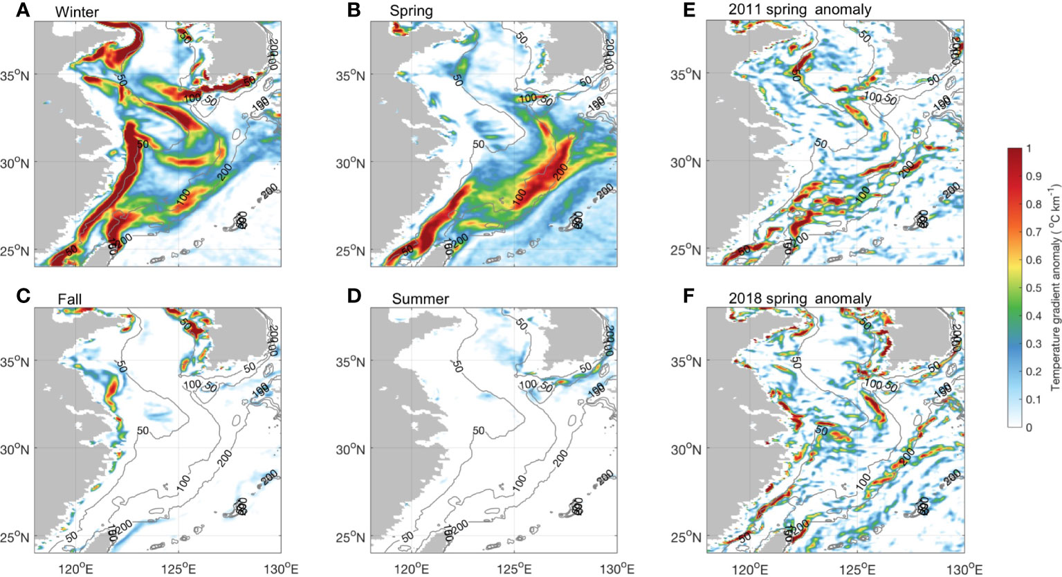
Figure 12 Seasonal anomalies of the temperature (SST) gradient, which are the differences between the mean SST gradient for each season and the annual mean SST gradient: (A) winter (December–February), (B) spring (March–May), (C) fall (September–November), and (D) summer (June–August). (E) 2011 spring SST gradient anomaly. (F) 2018 spring SST gradient anomaly. The gray contour lines in each map denote the 50-, 100-, and 200-m isobaths.

Another possible physical process that should be mentioned is the impact of cross-shelf penetrating fronts, which play an important role in the cross-shelf transport of coastal materials, including nutrients and chlorophyll, to the ECS shelf. Observations have suggested that cross-shelf transport is associated with frontal activities induced by instabilities in ocean currents (Glenn et al., 1996; Li et al., 2003; Yuan et al., 2005; Wu, 2015). The collision of wind-forced coastal jets with the TWC has been suggested as one of the mechanisms that generate cross-shelf penetrating fronts (He et al., 2010). A rather high occurrence of penetrating fronts during the prolonged La Niña event of 1999–2001 was observed in the ECS (He et al., 2010). This is consistent with our EOF-identified Chl-a anomaly in the same region and the close correlation between Chl-a, wind, and the ENSO index.

The impact of climate variability on the ECS

The observed Chl-a spatial and temporal interannual variabilities in the ECS were most likely due to forcing changes driven by a number of interacting climate cycles (e.g., MJO, ENSO, and PDO). These climate signals are more visible in the southern ECS than in the north, which could be associated with the influence of Kuroshio-induced air–sea interactions along its path (Zhang and Li, 2020) and the remote influences from the equatorial Indian and Pacific Oceans through atmospheric circulation and moisture transport (Chen et al., 2020). The southern ECS is separated from the Yellow Sea in the north by an area strongly influenced by the CDW. The influence of the CDW can extend to the northern edge of the triangular area identified in this study. The riverine input of color dissolved organic matter (CDOM) and total suspended matter increases the uncertainties in ocean color data to determine Chl-a variability (Bowers et al., 2011); thus, we need to be very careful when interpreting the riverine influence of Chl-a.

Possible ecosystem impact

While the seasonal Chl-a concentration within the southern ECS triangle region identified in this study is relatively small compared to the coastal area, its wide range and pronounced Chl-a interannual anomalies beyond the seasonal variation make its contribution significant. Phytoplankton are connected to higher trophic levels, with the ability to influence zooplankton (e.g., jellyfish) and, thus, the larger marine ecosystem through trophic cascades (West et al., 2009). Several studies have indicated that jellyfish blooms in coastal waters have increased significantly and become a marine environmental issue in the ECS (Dong et al., 2010; Xu et al., 2013b; Zhang et al., 2017). Phytoplankton and environmental temperature can affect jellyfish growth and metabolism in terms of food supply and polyp strobilation (Richardson et al., 2009). The co-occurrence of anomalously high temperature and high primary productivity or anomalously low temperature and high primary productivity could have different effects on higher trophic levels, thus influencing the food web structure. This provides an ideal setting for studying the associations between and responses of ecosystems to environmental factors.

Conclusions

EOF analysis was used to compress the spatiotemporal phytoplankton variability over the highly heterogeneous ECS area during the MODISA and SeaWiFS periods. The strong influences of wind, NHF, and PAR on EOF mode 1 temporal variability reflect the role of the onset of stratification as a driver of phytoplankton seasonality. Increasing incident light, temperature, and reduced mixing in spring resulted in mixed layer shallowing such that the spring bloom was initiated. Our results also demonstrate that substantial interannual variability in Chl-a exists in a triangular area in the southern ECS surrounded by three major SST fronts. While this region is characterized by low Chl-a, remarkable variability in Chl-a could result in ecosystem structure change because Chl-a is produced by phytoplankton and its concentration builds on the basis of the oceanic food chain. An integrated evaluation of the relationships between Chl-a and climate-sensitive local environmental variables (SST, wind, NHF, and PAR) suggests that Chl-a anomalies are in response to variability in basin-scale forcings. The PDO/ENSO is negatively correlated with Chl-a anomalies in most of the Kuroshio water area and positively correlated with Chl-a anomalies in much of the triangular area. In this area, significant Chl-a increases exist in negative PDO and ENSO modes (e.g., 2010–2011) with lower than normal SST, NHF, and PAR, but higher wind mixing. Anomalously high Chl-a is also present in the positive PDO and ENSO (e.g., 2018) when SST, NHF, and PAR are higher than normal, but wind stress is weaker. This finding suggests that different mechanisms regulate phytoplankton productivity. The Chl-a in-phase variability with PDO/ENSO probably reflects a local stratification-driven phytoplankton bloom, whereas the out-of-phase variability with PDO/ENSO indicates mixing driven by new nutrient sources, for example, more front activities and vertical mixing, which are associated with enhanced northerly winds. The strategy used in the present study promoted biologically relevant regionalization of the study area, improving our comprehensive understanding of phytoplankton driving forces over this highly heterogeneous ECS.

Data availability statement

Publicly available datasets were analyzed in this study. This data can be found here: https://oceancolor.gsfc.nasa.gov, https://cds.climate.copernicus.eu/cdsapp#!/dataset/.

Author contributions

YX: Conceptualization, Methodology, Formal analysis, Investigation, Writing - Original Draft, Funding acquisition. YW: Discussion, Reviewing and Editing. PX: Discussion, Reviewing and Editing. JG: Discussion, Reviewing and Editing. JZ: Supervision, Project administration, Reviewing and Editing. All authors contributed to the article and approved the submitted version.

Funding

This study was supported by a grant from the National Natural Science Foundation of China through Grant Nos. 41606025 and 41876074. The SeaWiFS and MODISA data were acquired from the https://oceancolor.gsfc.nasa.gov; the WOA18 data are provided by the NOAA National Centers for Environmental Information.

Conflict of interest

The authors declare that the research was conducted in the absence of any commercial or financial relationships that could be construed as a potential conflict of interest.

Publisher’s note

All claims expressed in this article are solely those of the authors and do not necessarily represent those of their affiliated organizations, or those of the publisher, the editors and the reviewers. Any product that may be evaluated in this article, or claim that may be made by its manufacturer, is not guaranteed or endorsed by the publisher.

Supplementary material

The Supplementary Material for this article can be found online at: https://www.frontiersin.org/articles/10.3389/fmars.2022.951395/full#supplementary-material

References

Andres M., Park J.-H., Wimbush M., Zhu X. H., Nakamura H., Kim K., et al. (2009). Manifestation of the pacific decadal oscillation in the kuroshio. Geophysical Res. Lett. 36 (16):L16602. doi: 10.1029/2009GL039216