Reconstruction of ocean temperature and salinity profiles in the Northern South China Sea using satellite observations

Based on historical temperature and salinity (T–S) profiles, the correlation between the sea surface temperature (SST) anomaly, sea surface dynamic height (SSH) anomaly, and temperature profile anomaly is constructed by regression analysis. A three-dimensional temperature field is reconstructed in the northern South China Sea by satellite SST and SSH, with daily temporal and 0.25°×0.25° spatial resolutions. The three-dimensional salinity field is also reconstructed based on the correlation between salinity and temperature. Compared with the observational T–S profiles, the reconstructed T–S field reflects the characteristics and structure and accurately describes the mesoscale variability of the ocean temperature field. The new expanded T–S field can be used as the initial field in numerical models and be assimilated into numerical reanalysis and prediction systems, improving their output.

1 Introduction

The northern South China Sea is a large marginal sea in the tropics with a maximum depth of over 5000 m and a variable temperature and salinity (T–S) structure with many mesoscale eddies, which mainly come from the unstable changes in the process of Kuroshio intrusion and wind stress curl changes (Wang et al., 2003; Su, 2004; Wu et al., 2007; Yuan et al., 2007; Hu and Hou, 2010). The T-S profiles of this region is the key database to study the eddy variation and other ocean processes.

At present, the availability of T–S observation profiles from Argo (Array for Real-time Geostrophic Oceanography), CTD (conductivity-temperature-depth), XBT (expendable bathythermograph), and ocean stations is increasing, especially the massive Argo observation profiles have played an essential role in the ocean observation system. For example, Nan et al. (2011) analysed the vertical structures of three long-lived anticyclonic eddies in the northern South China Sea by in situ measurements. Hu et al. (2012) demonstrated the penetration of nonlinear Rossby eddies into the South China Sea with cruise data. But real-time observation is still challenging, and the spatial resolution is low.

However, with the continued development of satellite remote sensing technology, sea surface temperature (SST) and sea surface dynamic height (SSH) datasets provide many real-time observations with high spatial resolution on the sea surface. For example, based on these satellite observations, detailed statistical characteristics of mesoscale eddies, including eddy census statistics, kinematic properties, shapes, nonlinearity and propagation characteristics, have been provided in many studies of the global ocean (Chaigneau et al., 2009; Chelton et al., 2011; Li et al., 2014; Li et al., 2016), especially for eddy-active regions like the South China Sea (Chen et al., 2011; Hu et al., 2011; Chen et al., 2012; Hu et al., 2012). However, satellite observations cannot provide any subsurface information. Therefore, the combination of in situ and satellite observation has become an effective method to reconstruct a more detailed ocean T–S field.

As early as the end of the 1980s, several methods for inverting T–S profiles by mapping sea surface information (SST or SSH) have been proposed. Hurlburt (1986) has constructed a numerical ocean model to transform simulated altimeter data into subsurface information dynamically. Studies and applications of satellite observations for inferring sea subsurface information matured using statistical methods (Carnes et al., 1990; Hurlburt et al., 1990; Carnes et al., 1994; Gavart and Mey, 1997; Pascual and Gomis, 2003), which are mainly based on empirical orthogonal functions (EOFs). These researchers showed that the deep sea or oceanic temperature and salinity profiles obtained by the combined inversion of SST and SSH is much better than the results using SST or SSH alone. Furthermore, Bruno and Santoleri (2004) used coupled pattern analysis to build the relationship between temperature profiles and sea surface information to rebuild the temperature field. The EOF and coupled pattern methods are simple and clearly reflect the physical concepts, but both require observation data with a certain continuity in time and space, which is limited in the actual ocean. Regression analysis is a data analysis method based on mathematical and statistical principles (Fox et al., 2002; Guinehut et al., 2004). First, a lot of statistics are mathematically processed, then a mathematical function expression (regression equation) with strong correlation is established by determining the correlation between the target variable and some independent variables, finally it is generalized to predict the possible changes of the dependent variable in the future. In this study, the regression analysis method was used to establish the mapping relationship between SST, SSH and temperature and salinity profiles using historical T–S profile observation data after strict quality control and fine processing for the northern South China Sea over a recent 30-year period. Then, the T–S profiles were reconstructed and examined. Compared with EOF and coupled pattern methods, althothg the regression analysis method lacks clear physical concept, it does not require time-space continuity of historical observation data, and the calculation method is simpler and more maneuverable (Fox et al., 2002).

This study is organised as follows. The historical and satellite observations used in this study are introduced in Section 2. In Section 3, the reconstruction of T–S profiles in the northern South China Sea based on the regression analysis method is described in detail. The results are examined using observed data, both in general and in case analyses. Finally, conclusions are summarised in Section 4.

2 Data and methodology

2.1 Historical argo profiles observations

The historical T–S profile data used in this study are based on the WOD18 (World Ocean Database, 2018) produced by the NODC (National Oceanographic Data Center), which mainly includes high-resolution CTD, XBT, DRB (drifting buoy), PFL (profiled buoy) and MRB (anchor buoy) data (Boyer et al., 2018). These data were supplemented by Argo float data obtained from the China Argo Real-time Data Center. The spatial range is from 110°E to 125°E, 15°N to 25°N, and the time range is from 1 January 1993 to 1 January 2018. The distribution of the Argo stations is shown in Figure 1, and they are spread throughout the northern South China Sea. Furthermore, quality control for this extensive profile dataset is essential to improve the accuracy of the results (Chaigneau et al., 2011). Thus, a valid database is constructed in several steps as follows:

1. Extract the required data including temperature, salinity, longitude, latitude, depth and date in the defined spatial and time range;

2. Delete data with NaN (not a number) values;

3. Select the data with a temperature between 0°C and 35°C and salinity between 31 psu and 36 psu;

4. Delete stations with less than three values in the vertical direction;

5. Construct a database with the standard vertical layer by linear interpolation for depths of 0, 5, 15, 20, 25, 30, 35, 50, 75, 100, 125, 150, 175, 200, 250, 300, 350, 400, 450, 500, 600, 700, 800, 900, 1000, 1100, 1200, 1300, 1400 and 1500 m.

FIGURE 1

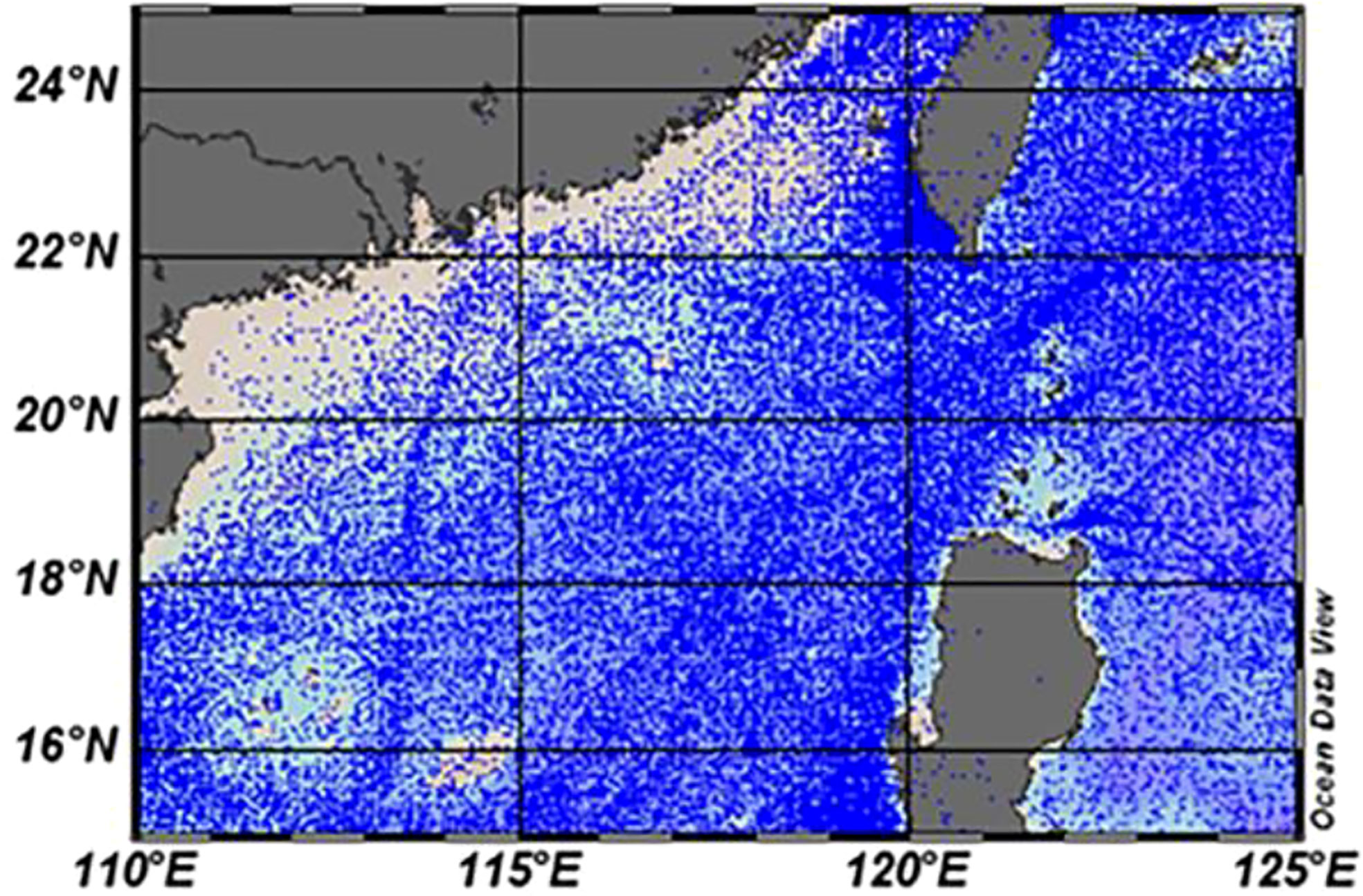
Figure 1 Distribution of observed T–S profile stations in the northern South China Sea.

Although the WOD18 data provides very high vertical resolution data, it was found in the process of data screening that the profiles change very little at depths below 500m and the profiles above 500m are highly variable. Furthermore, most ocean processes and phenomena are concentrated above 1500m, such as eddies, material transport. Therefore, we divided a total of 20 layers between the sea surface and 500m, which is basically the same as WOD18 data. However, the deep water layer with no obvious change were divided into 10 layers from 500m to 1500m, which would not affect the overall research results, and reduce a lot of calculation in the regression statistical analysis.

2.2 Climatic T–S data

The climatic T–S data based on the WOA18 (World Ocean Atlas, 2018) from NODC were regarded as an initial field and compared with the reconstructed results (Garcia et al., 2019). The WOA18 dataset provides standard layer data that have been objectively analysed. The spatial resolution is 1°, and the temporal sampling includes both annual average and monthly average versions. Comparing the reconstructed fields to these data can indicate T–S anomalies caused by eddies in the three-dimensional structure because the WOA18 data are excessively smoothed, and the eddy signals are significantly suppressed.

2.3 Test T–S data

The test T–S data were obtained from GTSPP(Global Temperature and Salinity Profile Plan) and Argo datasets. A total of 18.174 million T-S observation profiles have been provided by GTSPP from 1990 to 2014. The datasets mainly include XBT, which has strong timeliness and can be downloaded from NODC website. The Argo dataset includes the global Argo dataset and the Chinese Argo dataset, which collectively provide more than 1.4 million T-S observation profiles and can be downloaded from the China Argo Real-time Data Center website. These test data were subjected to strict quality control and then interpolated to the standard layer for the test. The observation profiles used for the test were not used during the reconstruction process and were strictly independent.

2.4 Satellite observations

The SST data used in this study are from a dataset provided by American Remote Sensing Systems (ARSS) that combines several observations from the optimal interpolation MW (microwave) and IR (infrared) sensors (Gentemann et al., 2010), including the TRMM (Tropical Rainfall Measuring Mission) Microwave Imager, AMSR-E, AMSR-2 (Advanced Microwave Scanning Radiometer), WindSat and MODIS (Moderate Resolution Imaging Spectroradiometer). The spatial resolution is 9 km, and the temporal sampling is 1 day. Moreover, the SSH data from DUACS (Data Unification and Altimeter Combination System) DT2014 from 1993 to 2018 with a spatial resolution of 0.25° and temporal sampling of 1 day (Pujol et al., 2016) were used in this study. It is provided by AVISO (Archiving, Validation and Interpretation of Satellite Oceanographic) and the datasets combined data from several altimeters, including T/P (Topex/Poseidon Satellite), ERS-1&2 (European Remote Sensing satellites 1&2), Jason-1&2, EnviSat (Environmental Satellite) and GFO (Geo Follow-On), which could be downloaded from the Copernicus Marine Environment Monitoring Service (CMEMS). And the sea level anomaly (SLA) data used in this study from multi-satellite altimeter is also provided by AVISO and has the same resolution as the SSH data, which could be downloaded from the CMEMS (Taburet et al., 2019).

2.5 Reconstruction of temperature profiles by SST and SSH

At present, there are three regression models for retrieving three-dimensional temperature field from sea surface information: The polynomial of SST, the polynomial of SSH, and the polynomial of the combination of SST and SSH are used. The third polynomial is a good combination of the two satellite observation data of SST and SSH. Previous studies have pointed out that the three-dimensional ocean temperature profile obtained by the joint inversion of SST and SSH is better than the profile obtained by the inversion of SST or SSH alone (Guinehut et al., 2004), so the polynomial combined with SST and SSH is directly used in this paper.

First, the sea surface dynamic height at each location can be calculated from its T–S profile as:

$\begin{array}{ll}h=\underset{0}{\overset{H}{\int }}\frac{\left[\nu \left(T,S,P\right)-\nu \left(0,35,P\right)\right]}{\nu \left(0,35,P\right)}dz& (1)\end{array}$

where ν is the seawater specific volume, ν(0,35,P) is the specific volume of seawater at 0°C temperature and 35 psu salinity, and H is the sea depth. Then, the correlation between the SST, SSH and the temperature profiles are established by regression analysis, expressed as:

$T_{i,k}\left(SST,h\right)=\overline{T_{i,k}}+a_{i,k}^{T3}\left(SST-\overline{T_{i,1}}\right)+a_{i,k}^{T4}\left(h-\overline{h_i}\right)$

$\begin{array}{ll}+a_{i,k}^{T5}\left[\left(SST-\overline{T_{i,1}}\right)\left(h-\overline{h_i}\right)-\overline{hSS{T}_i}\right]& (2)\end{array}$

WhereT_i,k(SST,h) are the values of the reconstructed temperature for extended grid point i and depth k,$\overline{hSS{T}_i}$is the weighted mean of the product, $\left(ss{t}_j-\overline{T_{i,1}}\right)$ $\left(h_j-\overline{h_i}\right)$, j  is the observation index, i is the location index, and $a_{i,k}^{T3}$,$a_{i,k}^{T4}$ and $a_{i,k}^{T5}$ are regression coefficients, they can be calculated by statistical method (Fox et al., 2002). The regression coefficients in equation (2) are obtained at monthly timescale, by comparing the monthly static climatic fields calculated from WOD18 to monthly-averaged satellite observations, the 3D T/S fields at daily time scale can be reconstructed by satellite daily resolution.

It is important to note that we only took one kind of polynomial of the structure, but the regression coefficients in each layer were determined by the plenty of T–S data, which are different in each layer. Therefore, the temperature field extended from Equation (2) is relatively independent in each vertical layer, which can better reflect the different variation characteristics of the actual temperature profile.

2.6 Reconstruction of salinity profiles by temperature

The correlation between the temperature and salinity can be expressed using Equation (3) by regression analysis:

$\begin{array}{ll}{S}_{i,k}\left(T\right)=\overline{S_{i,k}}+a_{i,k}^{S1}\left(T-\overline{T_{i,k}}\right)& (3)\end{array}$

where $\overline{S_{i,k}}$ is the average salinity, $\overline{T_{i,k}}$ is the average temperature and S_i,k(T) are the values of reconstructed salinity for grid point i and depth k , and $a_{i,k}^{S1}$ are the regression coefficients. Equation (3) was used to reconstruct the daily salinity profile data.

3. Results and discussion

3.1 Construction of the static climatic T–S field

Based on the WOD18 data, the historical temperature profile observations in the northern South China Sea were gridded and pre-treated using Equation (4) to form a static climate temperature field product with a horizontal resolution of 0.25° and a time scale of 1 month. It should be noted that the spatial resolution of 0.25° was seleted to be consistent with the satellite data, so as to complete the reconstruction.

$\begin{array}{ll}{T}_{i,k}^c=T_{i,k}^{WOA18}+\sum _{j=1}^{j=N}{w}_{i,j}\left(T_{j,k}^0-T_{j,k}^{WOA18}\right)& (4)\end{array}$

where $T_{j,k}^{WOA18}$ are the WOA18 temperature interpolated to the required position and depth, $T_{j,k}^0$ are the observation data, $T_{i,k}^c$ are the results at the new grid i and depth k . The w_i,j , N weights are calculated using Equation (5),

$\begin{array}{ll}{C}_i{W}_i=F_i& (5)\end{array}$

where w_i,j are weight coefficients, C_i is the covariance matrix and F_i is the matrix of initial errors between the grid point and the observation point. The calculation of Equations (5) is explained very clearly by Fox et al. (2002), which determined the w_i,j and then completed calculation of $T_{i,k}^c$.

The monthly vertical distribution of the northern South China Sea temperature profiles using these static climate field products is shown in Figure 2. Compared with the results from WOA18, the obtained temperature profiles are slightly different, especially at depths below 600 meters, where temperatures are about 0.3°C higher than the WOA18 temperatures. However, for depths above 600 meters, the temperature of the static climatic field is similar to WOA18. Figure 3 shows the vertical distribution of the temperature profile standard deviations. The values increase from the sea surface with increasing depth and reached a maximum of about 1.8 to 2.2°C near the thermocline in different months. Then temperature standard deviations gradually decrease with increasing depth and approach the minimum of about 0.2°C when the water depth exceeds 1000 meters.

FIGURE 2

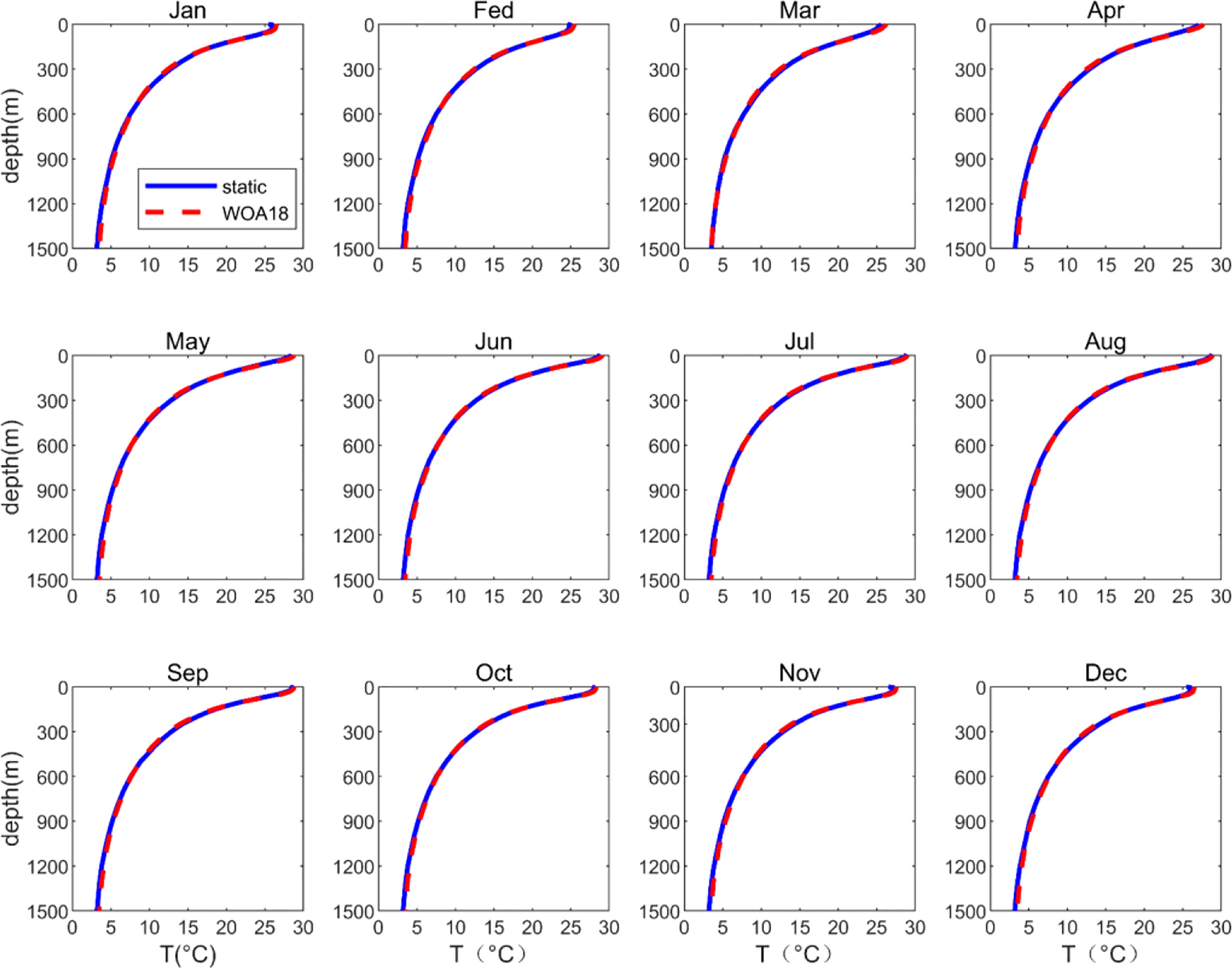
Figure 2 Monthly temperature profiles in the northern South China Sea. The blue and red lines represent the static climatic field and the WOA18 data, respectively.

FIGURE 3

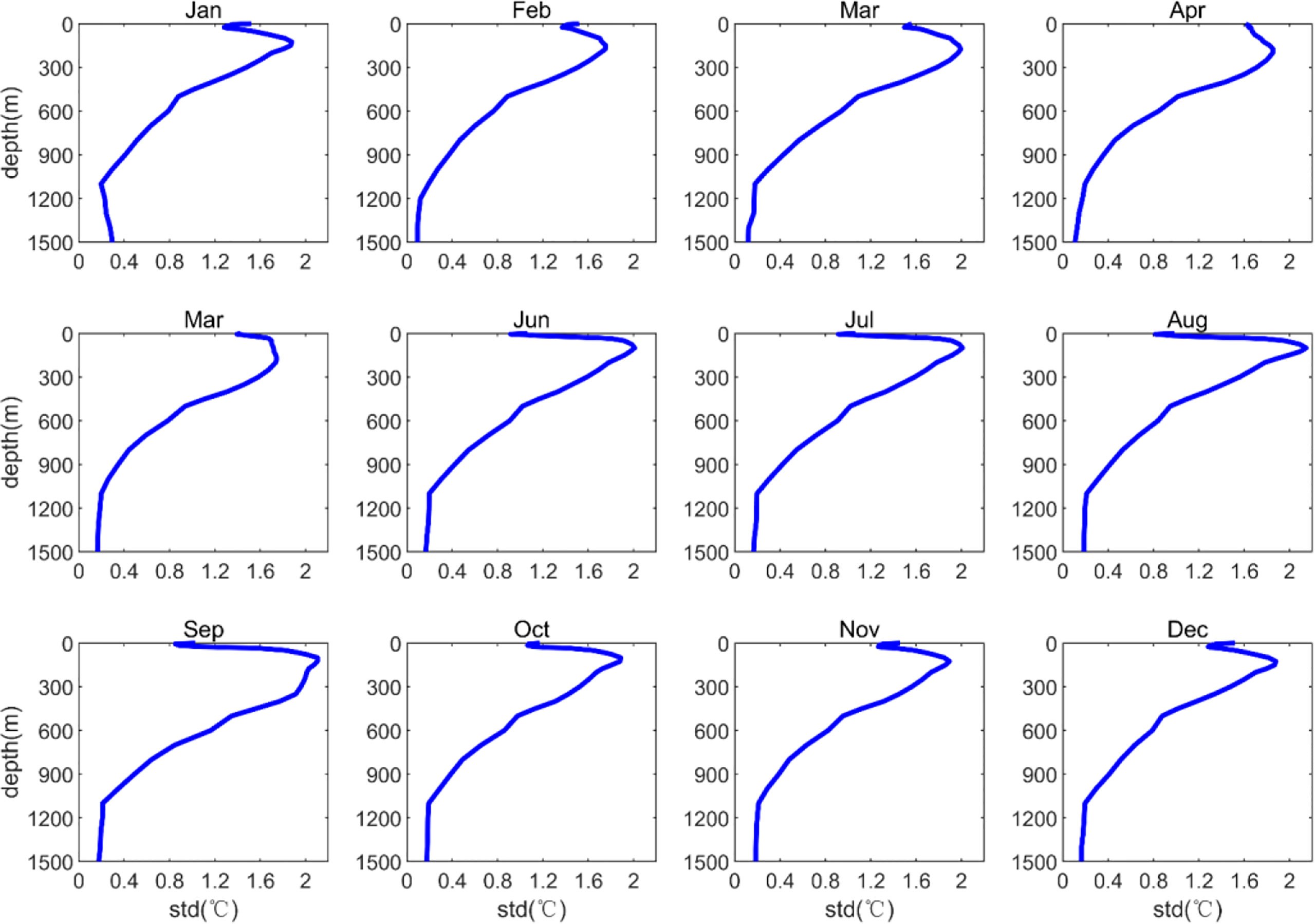
Figure 3 Vertical distribution of monthly static climatic temperature field standard deviations in the northern South China Sea.

Static climatic salinity fields were generated at each grid point based on Equation (3) for different water depths in the northern South China Sea. Similar to the temperature profiles, Figure 4 shows the monthly vertical distribution of the salinity profiles. The results were about 0.1 psu higher than the WOA18 data above 1000-meter depths and are highest near 400 meters. The two datasets are fairly consistent when the water depth exceeds 1000 meters. Figure 5 shows the vertical distribution of the salinity profile monthly standard deviations. The maximum standard deviation is about 0.3 psu at the surface. The salinity standard deviation drops sharply from the sea surface to about 400 meters depth and then maintains a low value of about 0.02 psu to the deepest data points.

FIGURE 4

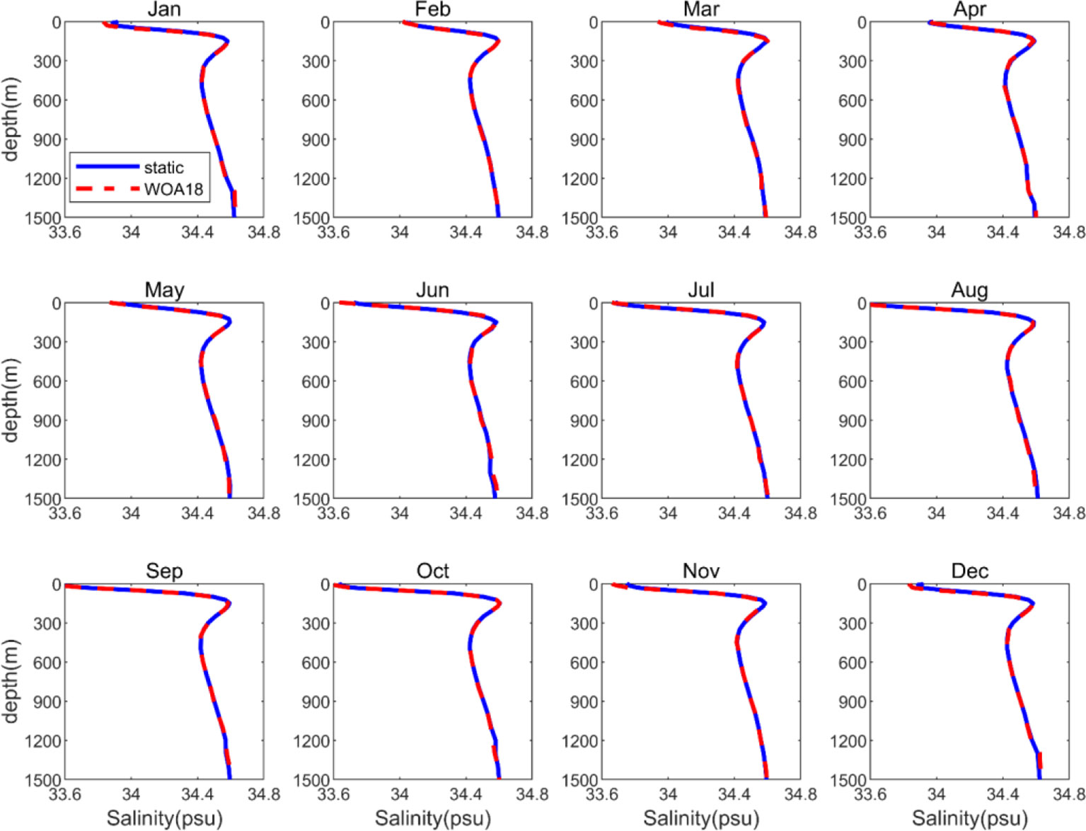
Figure 4 Monthly salinity profiles in the northern South China Sea. The blue and red lines represent the static climatic field and WOA18 data, respectively.

FIGURE 5

Figure 5 Vertical distribution of monthly static climatic salinity field standard deviations in the northern South China Sea.

3.2 Reconstruction of an expanded three-dimensional T–S field

3.2.1 Expanded three-dimensional T–S field and statistical tests

Based on Equation (2), the temperature static climate field in Section 3.1 was expanded to a three-dimensional temperature field with a spatial resolution of 0.25° and a daily time scale using the daily SST and SSH datasets. The three-dimensional salinity field with the same time and space resolution was also formed using Equation (3). Finally, the T–S observation data from GTSPP and Argo datasets in the northern South China Sea for a recent 20-year period were collated as a historical observation dataset for statistical testing.

The daily expanded three-dimensional T–S field data were interpolated to each observation position to obtain the corresponding expanded profiles, and the root–mean–square errors between the expanded results and the observation profiles were calculated month by month. Figures 6, 7 show the vertical distribution of the monthly errors of the expanded temperature and salinity profiles, respectively. The results show that the errors in monthly temperature are larger in the upper ocean and are over 1.0°C near the thermocline (100–200 meters), decreasing sharply with increasing depth below the thermocline. The errors reached their largest values (1.55°C) at a depth of 75 meters in July. Furthermore, the errors in monthly salinity are larger near the sea surface, reaching about 0.70 psu from June through October. With increasing depth, the values gradually decrease and then remain small below 200 meters. The T-S errors are close to the existing products called CORA (China ocean reanalysis), which was devoloped by similar method and its average errors of temperature (salinity) are 1.14°C (0.18 psu) (Han et al., 2011). In the future work, the integration of other data products may be an effective method to reduce the salinity profile errors at the sea surface (Yang et al., 2015; Bao et al., 2019).

FIGURE 6

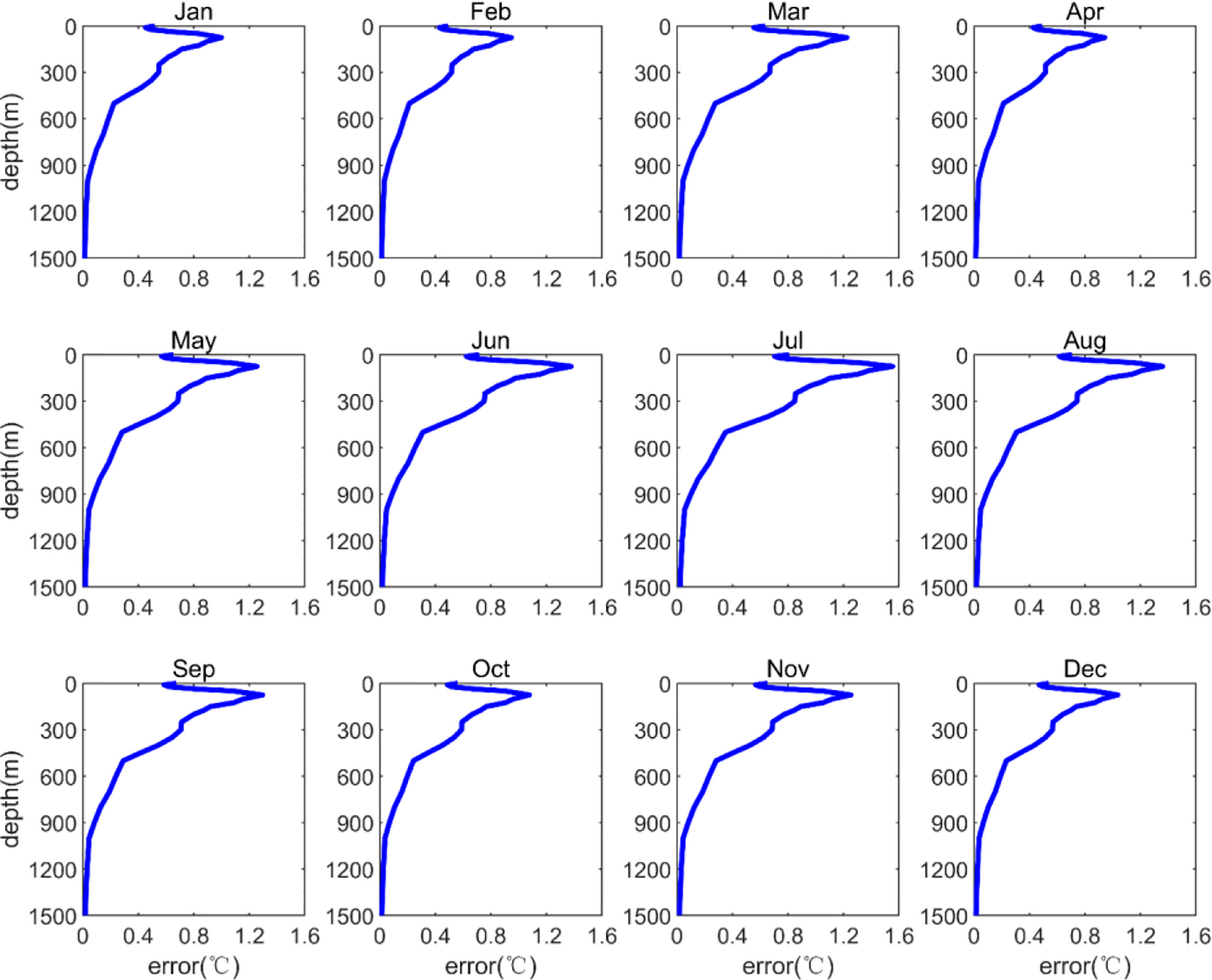
Figure 6 Vertical distribution of expanded temperature field monthly errors in the northern South China Sea.

FIGURE 7

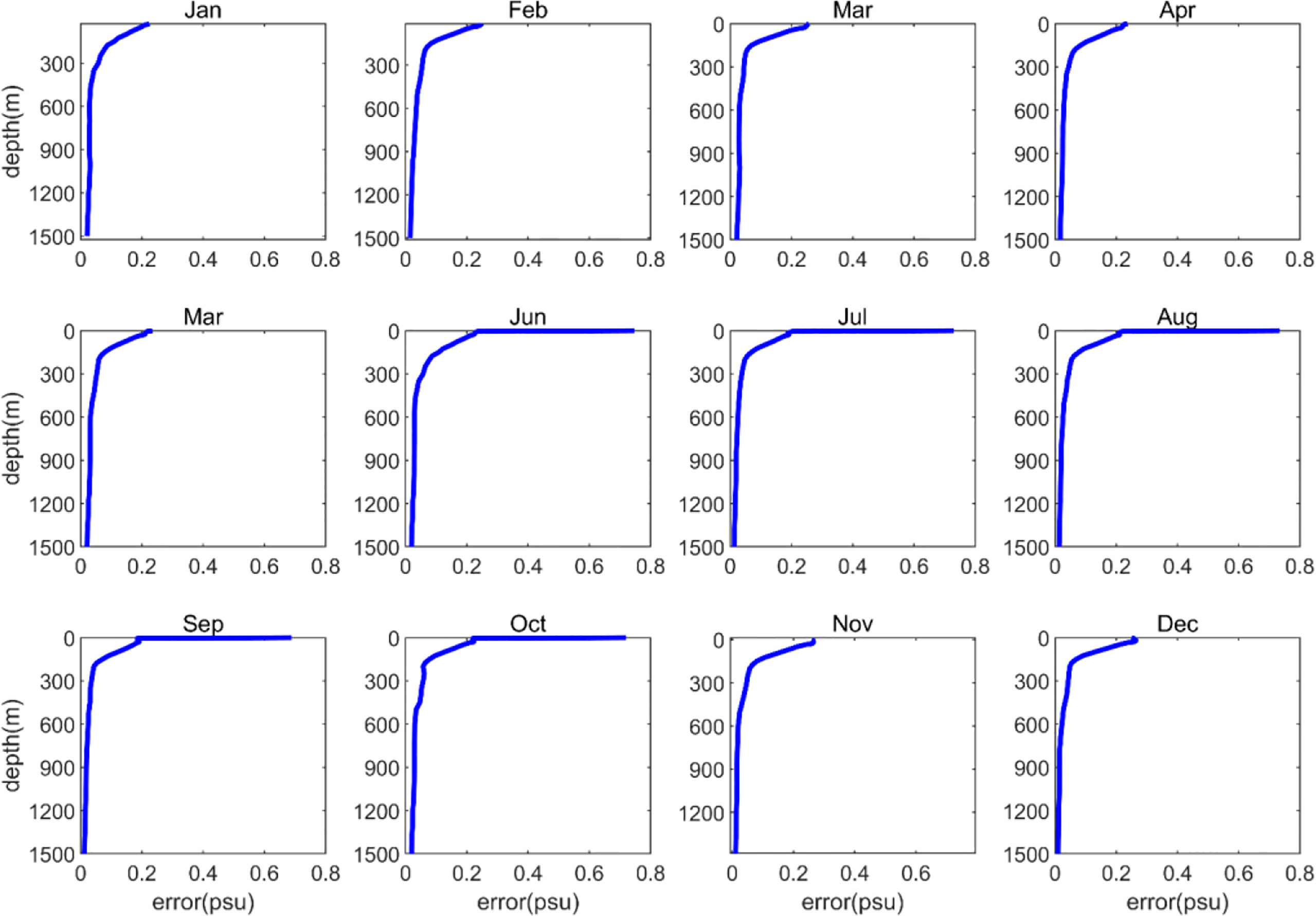
Figure 7 Vertical distribution of expanded salinity field monthly errors in the northern South China Sea.

3.2.2 Test of single stations

Stations 20110303 and 20110822 in Figure 8 were selected for further study. The expanded T–S profiles are compared with the observed data in Figure 9. The results show that the expanded profiles are very close to the observed profiles, proving that the expanded field can be effectively applied in this region. Furthermore, the spatial distribution of maximum temperature errors along the vertical showed in Figure 8, which revealed that the maximum errors increase near the coast of South China Sea.

FIGURE 8

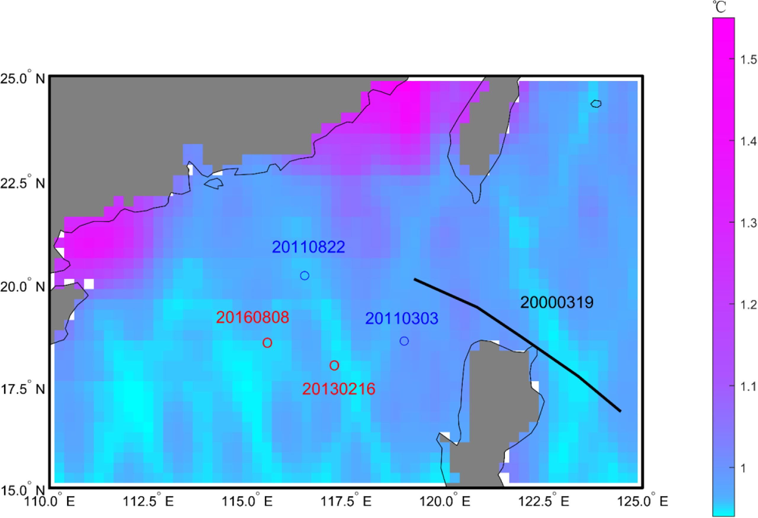
Figure 8 Two observation stations and a temperature cross-section. The numbers are dates and the background color is the spatial distribution of maximum temperature errors along the vertical.

FIGURE 9

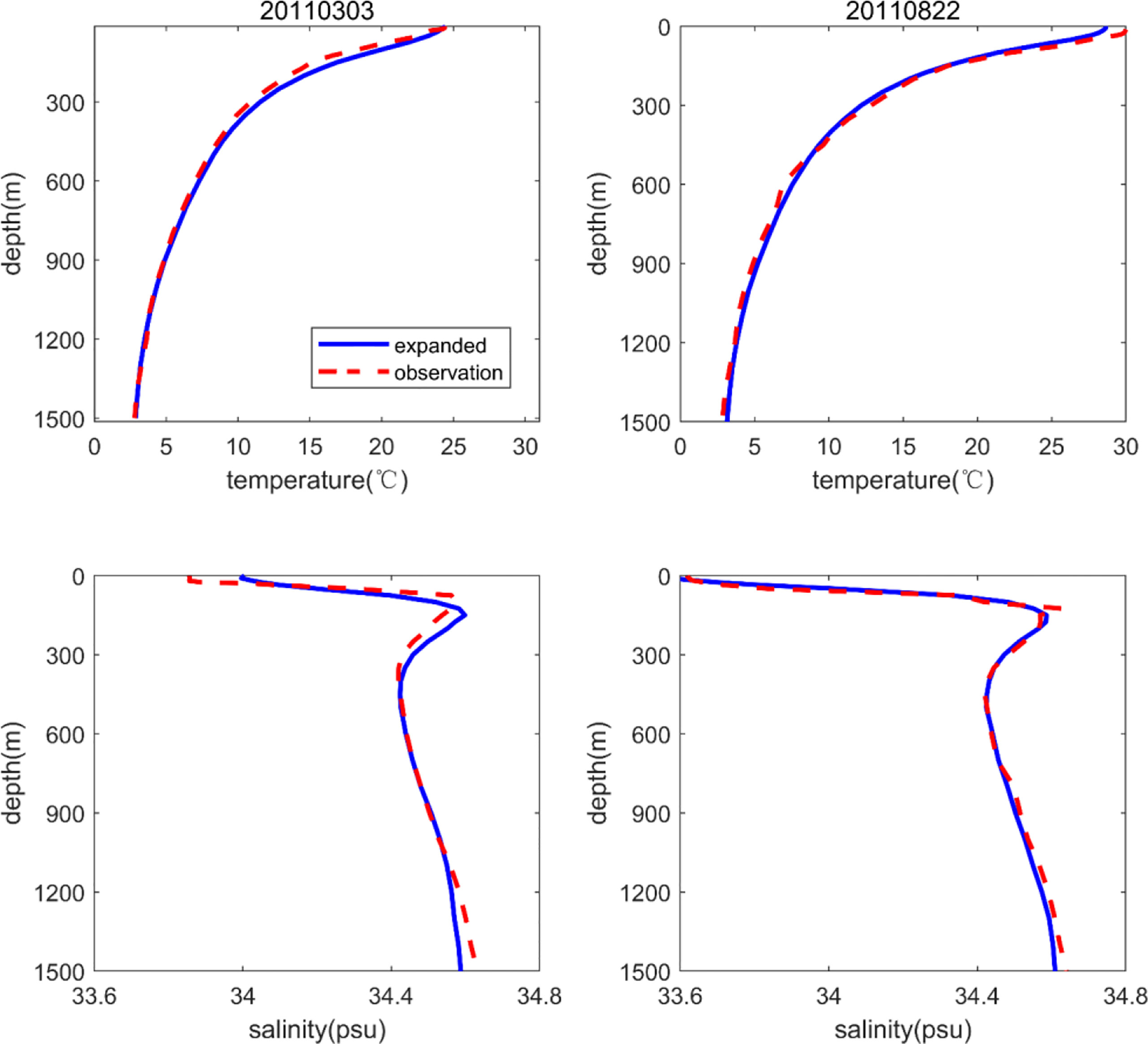
Figure 9 T–S profiles for two observation stations in the northern South China Sea. The blue and red lines represent the expanded T–S field results and observations (WOD18), respectively.

3.2.3 Cross-validation tests

The cross-validation tests were used for this work to strengthen the validation of the reconstruction. The WOD18 database was randomly divided into two parts in a ratio of 3 to 1, three quarters of them were used for the reconstruction method, and anothor part was kept for validation of the method.

Figures 10, 11 show the vertical distribution of the monthly errors of the expanded temperature and salinity profiles, respectively. The distribution of the errors results is similar to Figures 6, 7. The difference is that the errors obtained by cross-validation tests are generally small. For example, the temperature errors are generally less than 1.2°C (0.8°C) in summer (winter). The salinity errors are less than 0.2 psu overall, except in summer when it can reach 0.6 psu at the sea surface. The smaller errors may be due to the different databases used for validation.

FIGURE 10

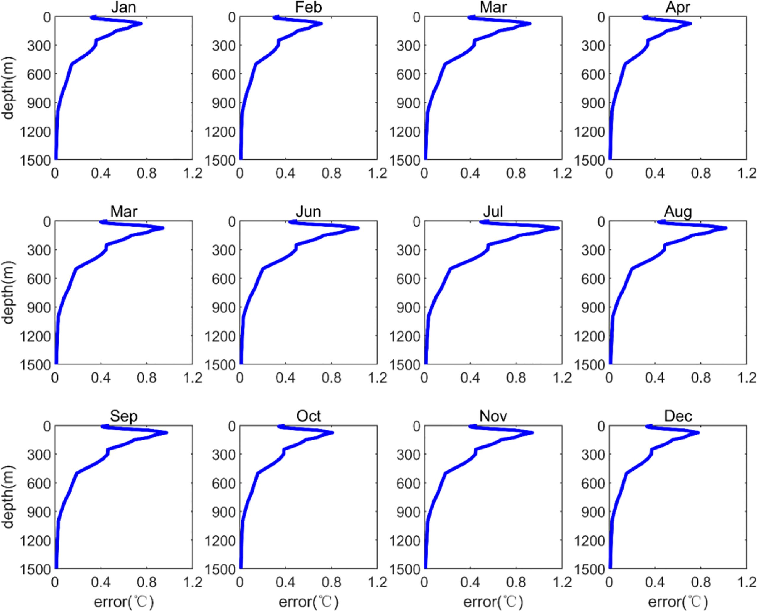
Figure 10 Vertical distribution of expanded temperature field monthly errors in the northern South China Sea (cross-validation tests).

FIGURE 11

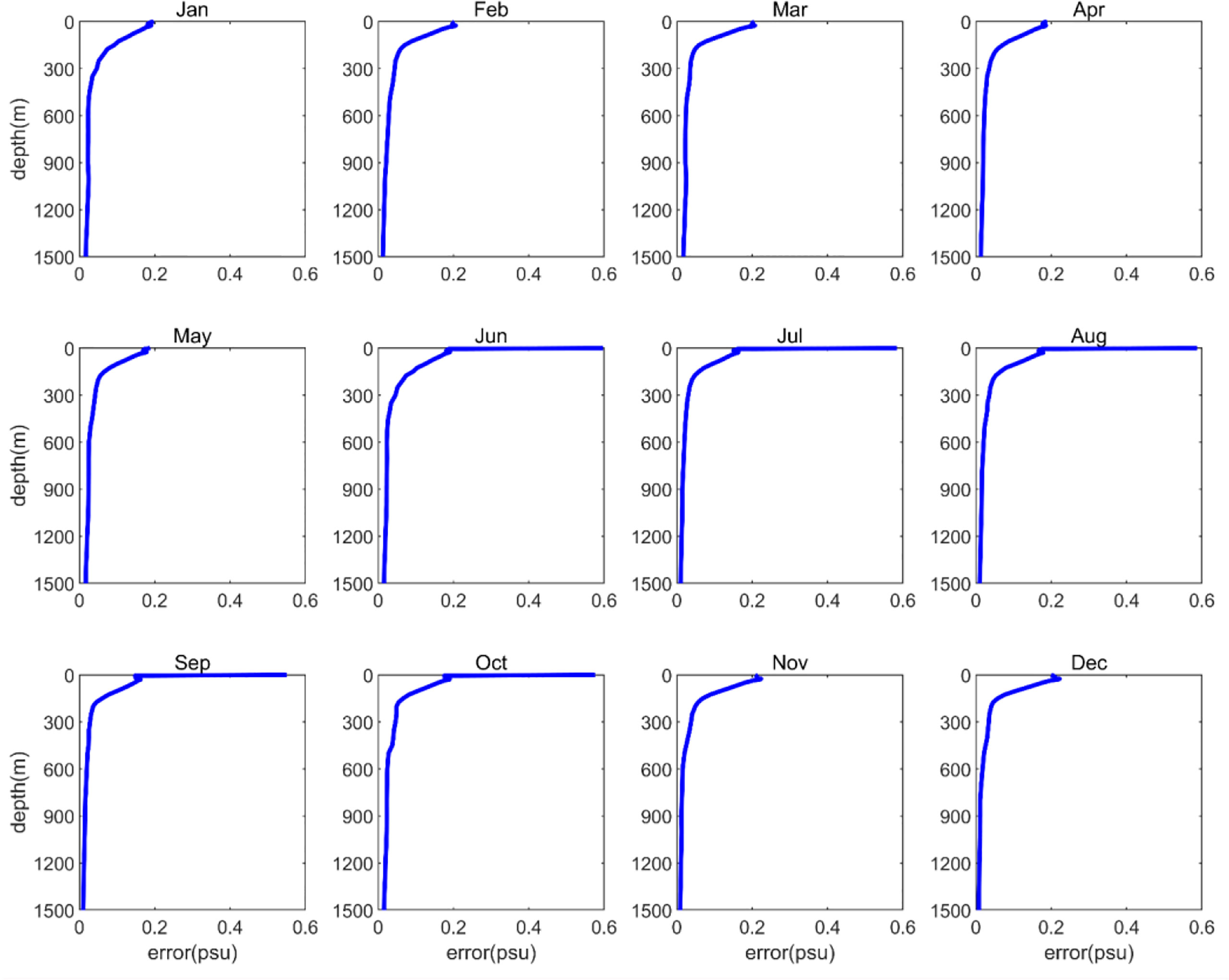
Figure 11 Vertical distribution of expanded salinity field monthly errors in the northern South China Sea (cross-validation tests).

Stations 20160808 and 20130216 in Figure 8 were selected for further study. The expanded T–S profiles are compared with the observed data in Figure 12. The results show that the expanded profiles are close to the observed profiles, proving that the expanded field can be verified by cross-validation tests.

FIGURE 12

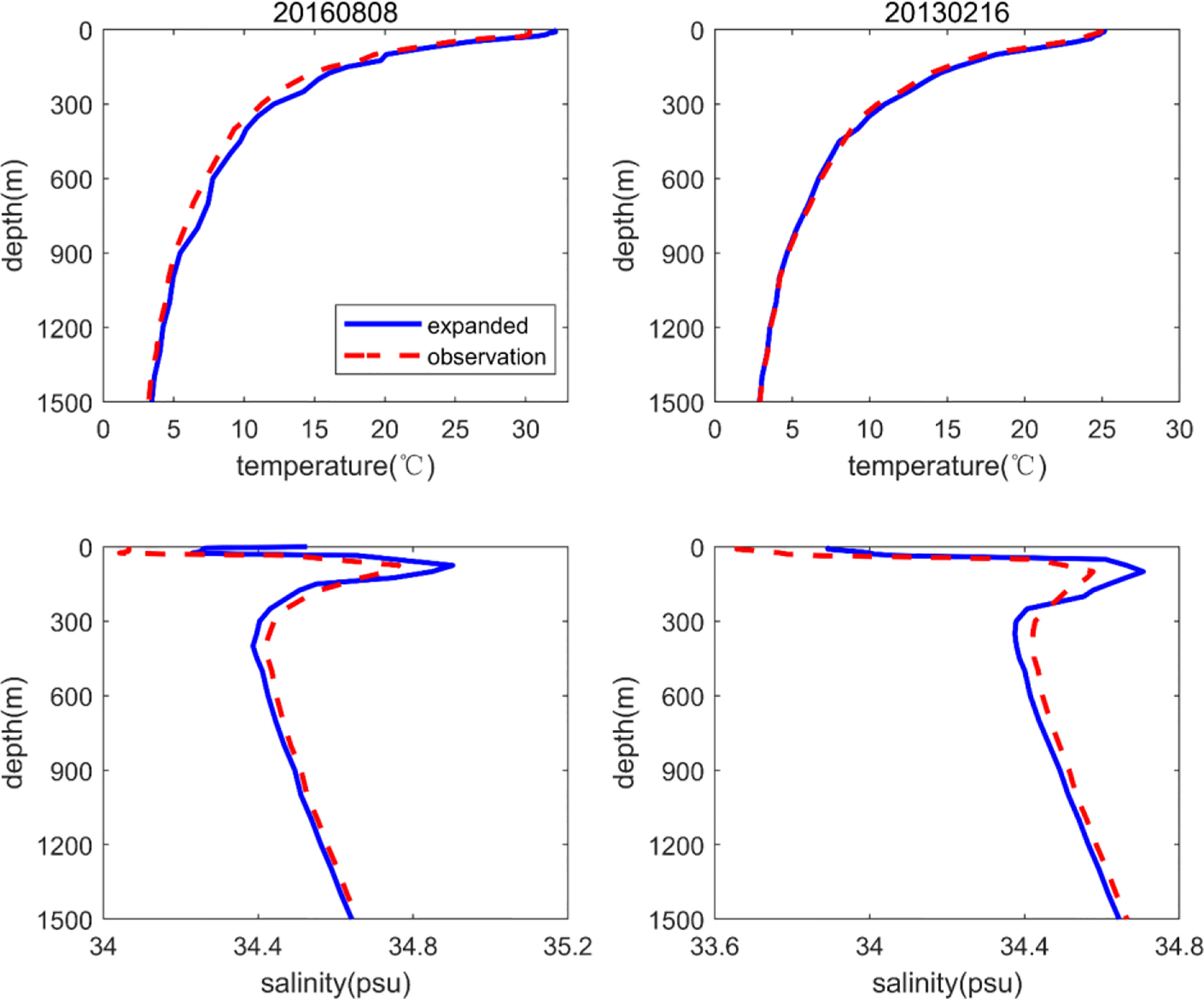
Figure 12 T–S profiles for two observation stations in the northern South China Sea (cross-validation tests). The blue and red lines represent the expanded T–S field results and observations (WOD18), respectively.

3.2.4 Comparison analysis of a temperature cross-section

An observation section between Taiwan Island and Luzon Island was selected to test the expansion results. The position of the observation section is shown in Figure 8. The starting position of the observation section is (118.0°E, 21.5°N), and the end position is (124.0°E, 16.5°N). The observation date is 19 March 2000. In the observed temperature section (Figure 13A), there is a cold eddy causing the isotherm to bulge upward near 122.0°E and a sinking isotherm caused by a warm eddy near 120.8°E and 123.3°E. Compared to the WOA18 climatic temperature section in March (Figure 13C), the expanded temperature section (Figure 13B) better reflects the internal variation characteristics of the mesoscale eddy. The two warm eddies in the observation section are well described, and the cold eddy is also shown. In addition, the structure of the upper mixed layer is further resolved.

FIGURE 13

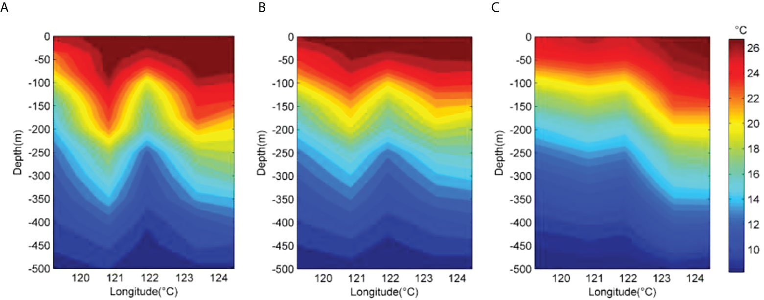
Figure 13 Temperature profiles of the cross-section (Figure 8) based on the observations (A), expanded temperature field (B) and WOA18 (C), respectively.

3.2.5 Structure and variation of the temperature profiles affected by the luzon warm eddy

The Luzon Warm Eddy (LWE) was first recognised as an anticyclonic ring centred at about 117.5°E, 21°N in summer (Li and Pohlmann, 2002). Yuan et al. (2007) used altimeter data to identify the ring as an anticyclonic eddy generated off the northwestern coast of Luzon Island and gave the LWE its name. The LWE is a seasonal phenomenon closely related to sea level anomalies (SLA). Figure 14 describes the variation of SLA during the LWE, and a black square was seleted as the target area. The results show that an anticyclonic eddy gradually formed a ring from 15 September 2006 through 5 November 2006, with high SLA in the target area. It then moved westward and finally disappeared on January 15, 2007 and the SLA in the target area decreased accordingly.

FIGURE 14

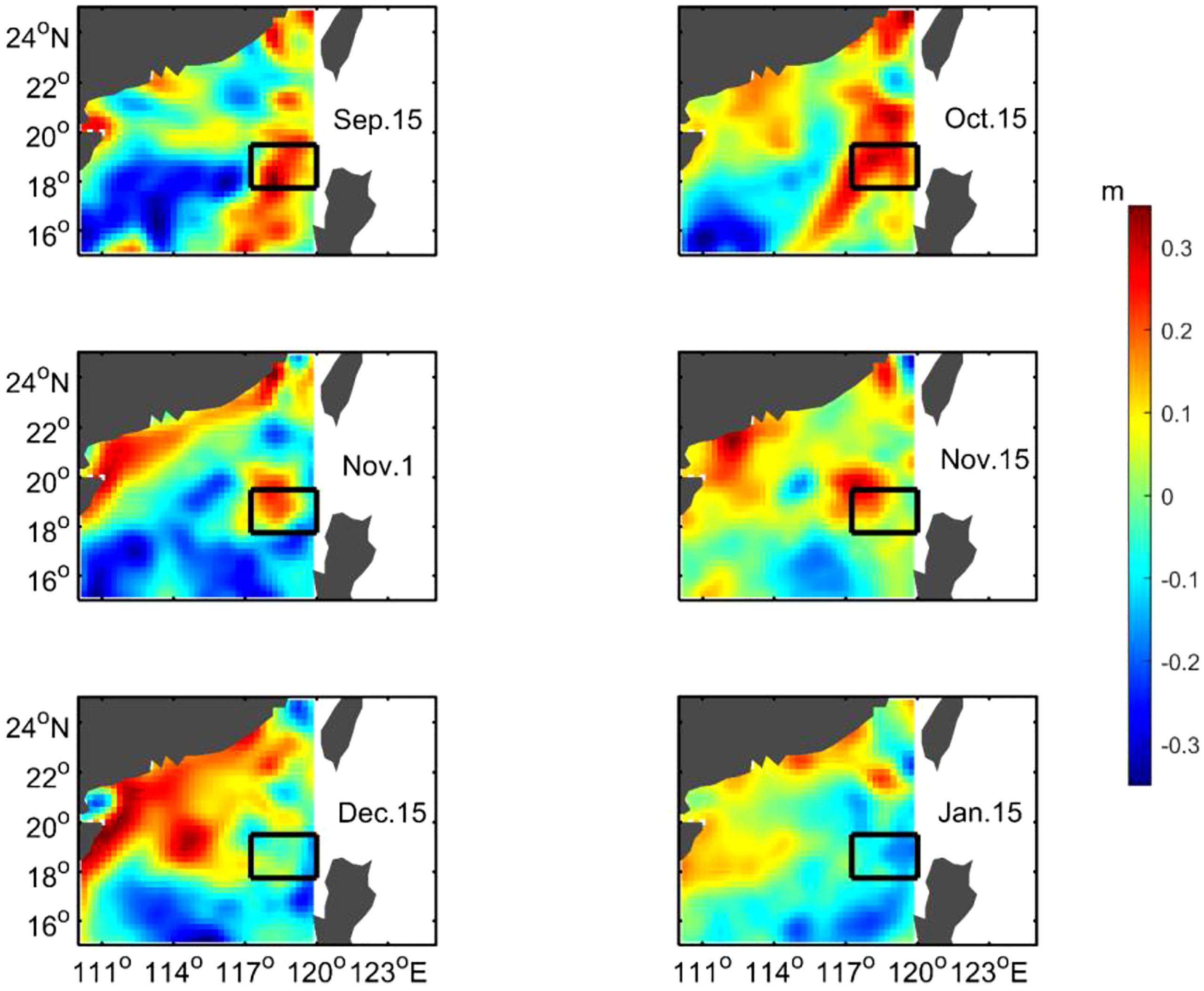
Figure 14 SLA (colours) from 15 September 2006 through 15 January 2007 in the western Luzon Strait. Black squares denote the locations of observed profiles from WOD18.

Figure 15 shows the time series of temperature profiles corresponding to the target area in Figure 14 based on the observation data and expanded temperature field, respectively. Similar to the observation data, the results for the expanded temperature field clearly show the variability of these temperature profiles. Because of the significant influence of the LWE, the upper-ocean temperatures were up to 28°C, and the thermocline depths were about 150 meters before November 2006. After the LWE had disappeared, the thermocline uplifted gradually, reaching 100 meters, and the upper-ocean temperatures were reduced to 22°C. In addition, the subtle time-scale changes were only reflected by observation data.

FIGURE 15

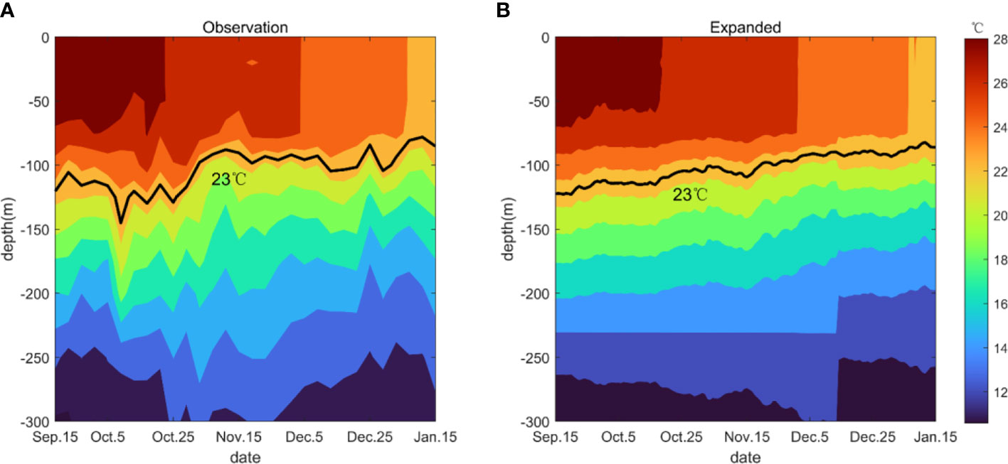
Figure 15 Temperature profiles corresponding to the black squares in Figure 14 based on the observation data (A) and the expanded temperature field (B), respectively. The black lines are isotherms of 23°C used as a thermocline proxy and the interval bewewen color contours is 2°C.

4 Conclusions

The mapping relationship between sea surface and subsurface temperature information was established by the linear regression analysis method using the historical Argo profile observations (WOD18). Daily three-dimensional temperature fields with a spatial resolution of 0.25° in the northern South China Sea were reconstructed based on the SST and SSH datasets derived from ARSS and CMEMS, respectively.

First, we selected valid data from WOD18 to construct a static climatic temperature field in the northern South China Sea and described their monthly vertical distributions. The results showed that these constructed temperature profiles were similar to the results from WOA18 and the standard deviations between them were relatively small, reaching a maximum of about 1.8°C near the thermocline and decreasing in other layers. The static climatic salinity fields were established next and were also close to the results from WOA18 with maximum standard deviations of about 0.3 psu at the surface.

An expanded three-dimensional T–S field was also reconstructed in the northern South China Sea. The T–S observation data from GTSPP and Argo datasets were selected as a statistical test field. The results showed that the monthly errors in the expanded temperature (salinity) profiles remained small and the maximum was less than 1.6°C (0.8 psu) near the thermocline (surface). Then, the errors of T-S profiles obtained by cross-validation were also smaller, and the maximun was less than 1.2°C (0.6 psu) near the thermocline (surface). Because of these small monthly errors, the expanded T–S fields are considered to provide a realistic representation of the northern South China Sea, and the expanded T–S profiles at two single stations were also confirmed to be similar to the observed results. Furthermore, the expanded T–S field clearly described the vertical temperature structure at a cross-section through the Luzon Strait and accurately simulated the structure and variation of the temperature profile associated with the LWE. These results prove that the ex-panded T–S field can accurately reflect the actual ocean field’s vertical structure and internal variation and the mesoscale eddies inside the ocean.

Obviously, the reconstructed salinity profiles have relatively large errors on the sea surface, especially in summer. Although this does not affect the overall results of this work, we hope to reduce the errors in future work. The use of satellite SSS (Sea Surface Salinity) database may be an effective method, which can provide large-scale and continuous data (Yang et al., 2015; Bao et al., 2019). Recently available SSS data mainly come from SMOS (Soil Moisture and Ocean Salinity), Aquarius and SMAP (Soil Moisture Active Passive) satellites, of which Aquarius stopped working on June 7, 2015 due to power supply problems (Tang et al., 2017). However, the SSS database is also required strict quality assessment and error analysis, and the data mainly focus on the last 10 years, so the use of SSS to complete the reconstructed salinity profile needs further research.

The T–S information inside the ocean is a basic component of oceanographic research data, playing a crucial role in describing the nature of the ocean. For example, Han et al. (2011) developed a regional ocean reanalysis system for the coastal waters of China and adjacent seas by similar method, and the evaluations show that a good representation of the processes and phenomena were produced. Wang et al. (2012) reconstructed the T-S profiles from 1993 to 2008 near the Luson Strait, which was used to estimate the heat, salt and volume transports during mesoscale eddies movement. This study’s expanded T–S field is expected to be used as the initial field for an ocean numerical model or for pseudo-observation assimilation into an ocean numerical reanalysis and prediction system to improve the three-dimensional T–S field results, which could delineate ocean processes and phenomena such as mesoscale eddies more clearly.

Data availability statement

Publicly available datasets were analyzed in this study. This data can be found here: NODC: https://www.nodc.noaa.gov/OC5/indprod.html; https://www.nodc.noaa.gov/gtspp/CARDC: ftp://data.argo.org.cn/pub/ARGO/raw_argo_data/; ftp://ftp.argo.org.cn/pub/ARGO/china/ARSS: http://www.remss.com/measurements/sea-surface-temperature CMEMS: http://marine.copernicus.eu.

Author contributions

Conceptualization, BT and DZ. Methodology, BT. Software, BT. Formal analysis, BT. Investigation, BT and DZ. Resources, BT. Data curation, DZ. Writing—original draft preparation, BT. Writing—review and editing, BT, DZ, CC and XZ. Visualization, BT, XZ and CC. All authors have read and agreed to the published version of the manuscript.

Funding

This research was supported by Research start-up fund of Qilu University of Technology, 81110727 and Shandong Provincial Natural Science Foundation, China, ZR202102240074.

Acknowledgments

The authors thank all agencies that provided the data. The authors are grateful for all the constructive comments from anonymous reviewers. The authors also thank the Editor for the kind assistances and beneficial comments.

Conflict of interest

The authors declare that the research was conducted in the absence of any commercial or financial relationships that could be construed as a potential conflict of interest.

Publisher’s note

All claims expressed in this article are solely those of the authors and do not necessarily represent those of their affiliated organizations, or those of the publisher, the editors and the reviewers. Any product that may be evaluated in this article, or claim that may be made by its manufacturer, is not guaranteed or endorsed by the publisher.

References

Bao S. L., Zhang R., Wang H. Z., Yan H. Q., Yu Y., Chen J. (2019). Salinity profile estimation in the pacific ocean from satellite surface salinity observation. J. Atmospheric Oceanic Technology. 36 (1), 53–68. doi: 10.1175/JTECH-D-17-0226.1

CrossRef Full Text | Google Scholar

Boyer T. P., Baranova O. K., Coleman C., Garcia H. E., Grodsky A., Locarnini R. A., et al. (2018). World ocean database 2018. Mishonov A. V. (Technical Editor, NOAA Atlas NESDIS 87). Available at: https://www.ncei.noaa.gov/sites/default/files/2020-04/wod_intro_0.pdf.

Google Scholar

Bruno B. N., Santoleri R. (2004). Reconstructing synthetic profiles from surface data. J. Atmospheric Oceanic Technology. 21, 693–703. doi: 10.1175/1520-0426(2004)021<0693:RSPFSD>2.0.CO,2

CrossRef Full Text | Google Scholar

Carnes M. R., Mitchell J. L., Dewitt P. W. (1990). Synthetic temperature profiles derived from geosat altimetry: Comparison with air-dropped expendable bathythermograph profiles. J. Geophysical Res. Atmospheres 95 (C10), 17979–17992. doi: 10.1029/JC095iC10p17979

CrossRef Full Text | Google Scholar

Carnes M. R., Teague W. J., Mitchell J. L. (1994). Inference of subsurface thermohlaline structure from fields measurable by satellite. J. Atmospheric Oceanic Technology. 11, 551–566. doi: 10.1175/1520-0426(1994)011<0551:IOSTSF>2.0.CO;2

CrossRef Full Text | Google Scholar

Chaigneau A., Eldin G., Dewitte B. (2009). Eddy activity in the four major upwelling systems from satellite altimetry(1992-2007). Prog. Oceanography. 83 (1), 117–123. doi: 10.1016/j.pocean.2009.07.012

CrossRef Full Text | Google Scholar

Chaigneau A., Texier M. L., Eldin G., Grados C., Pizarro O. (2011). Vertical structure of mesoscale eddies in the eastern south pacific ocean: A composite analysis from altimetry and argo profiling floats. J. Geophysical Res. 116, C11025. doi: 10.1029/2011JC007134

CrossRef Full Text | Google Scholar

Chelton D. B., Schlax M. G., Samelson R. M. (2011). Global observations of nonlinear mesoscale eddies. Prog. Oceanography. 91 (2), 167–216. doi: 10.1016/j.pocean.2011.01.002

CrossRef Full Text | Google Scholar

Chen G., Gan J., Xie Q., Chu X., Wang D., Hou Y. (2012). Eddy heat and salt transports in the south China Sea and their seasonal modulation. J. Geophysical Research-oceans 117, C05021. doi: 10.1029/2011JC007724

CrossRef Full Text | Google Scholar

Chen G., Hou Y., Chu X. (2011). Mesoscale eddies in the south China Sea: Mean properties, spatiotemporal variability, and impact on thermohaline structure. J. Geophysical Research-oceans 116, C06018. doi: 10.1029/2010JC006716

CrossRef Full Text | Google Scholar

Fox D. N., Teague W. J., Berron C. N., Carnes M. R., Lee C. M. (2002). The modular ocean data assimilation system. J. Atmospheric Oceanic Technology. 19, 240–252. doi: 10.1175/1520-0426(2002)019%3C0240:TMODAS%3E2.0.CO;2

CrossRef Full Text | Google Scholar

Garcia H. E., Boyer T. P., Baranova O. K., Locarnini R. A., Mishonov A. V., Grodsky A., et al. (2019) World ocean atlas 2018: Product documentation. Available at: https://data.nodc.noaa.gov/woa/WOA18/DOC/woa18documentation.pdf.

Google Scholar

Gavart M., Mey P. (1997). Isopycnal EOFs in the Azores current region: A statistical tool for dynamical analysis and data assimilation. J. Phys. Oceanography. 27, 2146–2157. doi: 10.1175/1520-0485(0)027<2146:IEITAC>2.0.CO;2

CrossRef Full Text | Google Scholar

Gentemann C. L., Meissner T., Wentz F. J. (2010). Accuracy of satellite sea surface temperatures at 7 and 11 GHz. IEEE Trans. Geosci. Remote Sensing. 48, 1009–1018. doi: 10.1109/TGRS.2009.2030322

CrossRef Full Text | Google Scholar

Guinehut S., Traon P. Y. L., Larnicol G., Philipps S. (2004). Combining argo and remote-sensing data to estimate the ocean three dimensional temperature fields-a first approach based on simulated observations. J. Mar. Systems. 46 (1-4), 85–98. doi: 10.1016/j.jmarsys.2003.11.022

CrossRef Full Text | Google Scholar

Han G. J., Li W., Zhang X. F., Li D., He Z. J., Wang X. D., et al. (2011). A regional ocean reanalysis syestem for China coastal waters and adjacent seas. Adv. Atmospheric Sci. 28 (3), 682–690. doi: 10.1007/s00376-010-9184-2

CrossRef Full Text | Google Scholar

Hu J., Gan J., Sun Z., Zhu J., Dai M. (2011). Observed three-dimensional structure of a cold eddy in the southwestern south China Sea. J. Geophysical Research-Oceans 116, C05016. doi: 10.1029/2010JC006810

CrossRef Full Text | Google Scholar

Hu P., Hou Y. (2010). Path transition of the Western boundary current with a gap due to mesoscale eddies: A 1.5-layer, wind-driven experiment. Chin. J. Oceanology Limnology. 28, 364–370. doi: 10.1007/s00343-010-9293-x

CrossRef Full Text | Google Scholar

Hurlburt H. E. (1986). Dynamic transfer of simulated altimeter data into subsurface information by a numerical ocean model. J. Geophysical Research-Atmospheres 91 (C2), 2372–2400. doi: 10.1029/JC091iC02p02372

CrossRef Full Text | Google Scholar

Hurlburt H. E., Fox D. N., Metzger J. (1990). Statistical inference of weekly correlated subthermocline fields from satellite altimeter data. J. Geophysical Research-Atmospheres 95 (C7), 11375–11409. doi: 10.1029/JC095iC07p11375

CrossRef Full Text | Google Scholar

Hu J., Zheng Q., Sun Z., Tai C. K. (2012). Penetration of nonlinear rossby eddies into south China Sea evidenced by cruise data. J. Geophysical Research-Oceans 117, C03010. doi: 10.1029/2011JC007525

CrossRef Full Text | Google Scholar

Li L., Pohlmann T. (2002). The south China Sea warm-core ring 94S and its influence on the distribution of chemical tracers. Ocean Dynamics. 52 (3), 116–122. doi: 10.1007/s10236-001-0009-9

CrossRef Full Text | Google Scholar

Li Q. Y., Sun L., Lin S. F. (2016). GEM: A dynamic tracking model for mesoscale eddies in the ocean. Ocean Science. 12 (6), 1249–1267. doi: 10.5194/os-12-1249-2016

CrossRef Full Text | Google Scholar

Li Q. Y., Sun L., Liu S. S., Xian T., Yan Y. F. (2014). A new mononuclear eddy identification method with simple splitting strategies. Remote Sens. Letters. 5 (1), 65–72. doi: 10.1080/2150704X.2013.872814

CrossRef Full Text | Google Scholar

Nan F., He Z., Zhou H., Wang D. (2011). Three long-lived anticyclonic eddies in the northern south China Sea. J. Geophysical Research-Oceans 116, C5. doi: 10.1029/2010JC006790

CrossRef Full Text | Google Scholar

Pascual A., Gomis D. (2003). Use of surface data to estimate geostrophic transport. J. Atmospheric Oceanic Technology. 20, 912–926. doi: 10.1175/1520-0426(2003)020%3C0912:UOSDTE%3E2.0.CO;2

CrossRef Full Text | Google Scholar

Pujol M. I., Faugère Y., Taburet G., Dupuy S., Pelloquin C., Ablain M., et al. (2016). DUACS DT2014: The new multi-mission altimeter data set reprocessed over 20 years. Ocean Science. 12, 1067–1090. doi: 10.5194/os-12-1067-2016

CrossRef Full Text | Google Scholar

Su J. (2004). Overview of the south China Sea cuirculation and its influene on the coatal physical oceanography outside the pearl river estuary. Continental Shelf Res. 24, 1745–1760. doi: 10.1016/j.csr.2004.06.005

CrossRef Full Text | Google Scholar

Taburet G., Roman A. S., Ballarotta M., Pujol M. I., Dibarboure G. (2019). DUACS DT2018: 25 years of reprocessed sea level altimetry products. Ocean Science. 15, 1207–1224. doi: 10.5194/os-15-1207-2019

CrossRef Full Text | Google Scholar

Tang W. Q., Fore A., Yush S., Lee T., Hayashi A., Sanchez F. A., et al. (2017). Validating SWAP SSS with in situ measurements. Remote Sens. Environment. 200, 326–340. doi: 10.1109/IGARSS.2017.8127518

CrossRef Full Text | Google Scholar

Wang X. D., Li W., Qi Y. Q., Han G. J. (2012). Heat, salt and volume transports by eddies in the vicinity of the Luzon strait. Deep Sea Research Part I 61, 21–33. doi: 10.1016/j.dsr.2011.11.006

CrossRef Full Text | Google Scholar

Wang G. H., Su J. L., Chu P. C. (2003). Mesoscale eddies in the south China Sea observed with altimeter data. Geophysical Res. Letters. 30 (21), 2121. doi: 10.1029/2003GL018532

CrossRef Full Text | Google Scholar

Wu C. C., Lee C. Y., Lin I. I. (2007). The effect of the ocean eddy on tropical cyclone intensity. J. Atmospheric Sci. 64, 3562–3578. doi: 10.1175/JAS4051.1

CrossRef Full Text | Google Scholar

Yang T. T., Cheng Z. B., He Y. J. (2015). A new method to retrieve salinity profiles from sea surface salinity observed by SMOS satellite. Acta Oceanologica Sinica. 34, 85–93. doi: 10.1007/s13131-015-0735-3

CrossRef Full Text | Google Scholar

Yuan D. L., Han W. Q., Hu D. X. (2007). Anti-cyclonic eddies northwest of Luzon in summer-fall observed by satellite altimeters. Geophysical Res. Lett. 34, L13610. doi: 10.1029/2007GL029401

CrossRef Full Text | Google Scholar