Changes in Distribution Patterns for Larimichthys polyactis in Response to Multiple Pressures in the Bohai Sea Over the Past Four Decades

Understanding patterns of change in the distribution of species among their critical habitats is important for analyzing population dynamics and adaptive responses to environmental shifts. We investigated spatio-temporal changes in small yellow croaker (Larimichthys polyactis) using eight alternative models fitted to data from bottom trawl surveys conducted in the Bohai Sea each spring (spawning period) and summer during 1982–2018. These models included different combinations of local sea temperature, fishing pressure, and individual climate index (i.e., North Pacific index, NPI, and West Pacific index, WPI) as explanatory variables. Selection of the most parsimonious model for each season was based on Akaike’s Information Criterion (AIC). The model with NPI as its only explanatory variable was used as a base case for pre-analysis. In spring, a spatio-temporal model with sea temperature as a quadratic effect, plus the spatially varying effects of a climate index and fishing pressure was selected, as the AIC value of this model was reduced by 41.491 compared to the base case model without these effects. In the summer after spawning, the spatio-temporal model with WPI as a climate index covariate lagged by 1-year best explained the spatio-temporal distribution patterns of the stock. The results suggested that small yellow croaker populations significantly decreased in biomass in the Bohai Sea over the study period. A statistically significant northeastward shift in the center of gravity (COG) and a contraction in the distribution range occurred in summer throughout the study period (p<0.05). During the spring sequence (1993–2018), a statistically significant northeastward shift in the COG was also found (p<0.05). Our results showed that biomass-density hotspots of small yellow croaker in both seasons have shrunk or disappeared in recent years. Overall, these findings suggest that the spatio-temporal patterns of the populations in their spawning, feeding and nursery grounds have been influenced over the past 40 years by multiple pressures, and population density in the southwestern areas of the Bohai Sea declined faster and more drastically than in the northeastern areas. This study has important implications for developing targeted spatial conservation measures for small yellow croaker at various stages of its life history under different levels of stress.

Introduction

Key ontogenetic habitats for fish populations (spawning grounds, nursery grounds, etc.) support their reproduction and continual replenishment, and are often areas subject to intensive human activities and high levels of exploitation. In the context of global environment change (increasingly intensified impacts of human activities exacerbating adverse climatic conditions), understanding the response mechanisms to environmental change among fish habitats is prerequisite for sustainable development of marine fisheries and protection of their supporting ecosystems (Lotze et al., 2006; Browman and Skiftesvik, 2014; Jin et al., 2015). Studies of sustainable fish production as marine ecosystems evolve under environmental stressors is at the forefront of contemporary fisheries research (Jin et al., 2015).

Tracking and understanding distribution shifts of fish stocks and patterns of expansion or contraction in their spawning, nursery, and feeding grounds is fundamental to effective fisheries management. This understanding can help fisheries scientists and managers to clarify the response mechanisms of stocks to environmental changes (Astarloa et al., 2021) and the downstream effects of these changes on the delivery of fisheries ecosystem services such as food production (Myers and Worm, 2003; Lotze et al., 2006; Cheung et al., 2013). In so doing, it facilitates the establishment of a scientific theoretical framework for ecosystem-based adaptive, and in some instances restorative, management of fisheries (Botsford et al., 1997; Pikitch et al., 2004; Beddington et al., 2007; Jin et al., 2015; Thorson, 2019a).

There is increasing evidence that anthropogenic pressures (e.g., fishing) have led to dramatic distribution changes in the critical habitats of many marine species populations (e.g., Liu et al., 1990; Engelhard et al., 2014; Han et al., 2021; Grüss and Thorson, 2019). Fishing can greatly reduce stock biomass and alter population structure (Li et al., 2012; Bell et al., 2015). It can also give rise to changes in life history characteristics and phenotypic evolution (Sun et al., 2022), typically leading to shrinkage or displacement of the area occupied by exploited fish populations (Engelhard et al., 2014; Bell et al., 2015). Seawater pollution caused by human activities can also seriously damage the functions of key habitats. Species diversity and abundance of fish eggs in polluted waters can become significantly reduced, leading to a narrowing and spatial shift in spawning grounds (Cui et al., 2003).

Environmental stressors (e.g., temperature changes, climate changes) can also lead to spatial shifts among fish stocks (e.g., Blanchard et al., 2005; Pinsky et al., 2013). Many studies have already shown that temperature change is the key factor that initiates migration between key habitats (Feng and Yang, 1955; Liu et al., 1990; Jin et al., 2005), and is also an important environmental determinant of stock distribution. Disruption of migration and restriction of habitable environments may make it difficult to obtain adequate catches from existing fishing grounds in the future (e.g., Overholtz et al., 2011; Cheung et al., 2013; Bell et al., 2015; Su et al., 2015). Water temperature also affects the survival, development and hatching of fish eggs (Bian et al., 2014), thereby causing fluctuations in population replenishment and changes in fish distribution. In some cases, species distributional shifts are related to the nature of climate change rather than increasing temperature per se (Pinsky et al., 2013). A study in the Bay of Biscay showed that the regional climate index provided a better explanation than local environmental variables (SST and chlorophyll) in the spatio-temporal distribution patterns of dolphins (Astarloa et al., 2021), although local effects may be more influential on the trophodynamics of teleosts than mammals.

Environmental stressors can also have profound indirect effects on the early life stages of marine fish in both nursery and feeding grounds. It has been found that long-term changes in the water temperature of the North Sea cod (Gadus morhua) habitat caused by global climate change has altered species composition, population structure and abundance of copepods that the cod larvae rely upon for food. High larval mortalities from their inadequate food supply, have consequently impaired stock recruitment giving rise to dramatic fluctuations and an overall decline in North Sea cod stocks over the last few decades (Beaugrand et al., 2003; Richardson et al., 2004). In many instances, depending on their specific life history stages, carnivorous fish populations are far less directly sensitive to temperature and other stressors than their planktivorous prey. Ignoring indirect effects from declines in prey may render exploited fish species without adequate protection and preclude their optimal utilization.

Critical habitats are increasingly recognized by researchers as being affected by combinations of multiple stressors. For example, climate warming and fishing pressure have combined to influence a century of distributional shifts of Gadus morhua in the North Sea (Engelhard et al., 2014). In China, multiple stressors have caused shifts in ecosystem structure and function during the spawning season in Laizhou Bay (Jin et al., 2013). Jin et al. (2013) showed that top-down effects have been the dominant influence on species composition over the last half century due to increased fishing pressure, whilst bottom-up effects have increased over the last thirty years due to strong changes in environmental stressors (other stressors such as temperature, nutrients, and salinity). These findings imply that fisheries scientists and managers need to identify and monitor the multiple stressors affecting fish populations to effectively manage exploited fish stocks.

The Bohai Sea is a semi-enclosed shallow sea in China’s warm temperate zone and is connected with the Yellow Sea to its east (Figure 1), which is a key habitat integrating spawning, nursery and fishing grounds (Liu et al., 1990). Many highly migratory fishes of the Yellow and Bohai Seas with high socio-economic importance spawn and forage in the Bohai Sea, with the latter playing a crucial role in replenishing most fish populations in the Yellow Sea Large Marine ecosystem (Jin et al., 2005; Jin et al., 2015; Bian et al., 2018). Small yellow croaker (Larimichthys polyactis, northern Yellow Sea-Bohai Sea stock) is the most iconic and important among exploited species in this region, relying on habitats in the Bohai Sea for its spawning and nursery phases of life before overwintering in the fishing grounds of the Yellow Sea (Liu et al., 1990). Despite the important implications of the relationship between small yellow croaker and multiple stressors during its spawning and nursery periods for stock conservation, scant research has been conducted on this topic. Therefore, there is an urgent need to better elucidate the patterns of variation in the spatial distribution of the stock in its spawning, nursery and feeding grounds of the Bohai Sea, how these patterns change over time, and how these patterns respond to variations in anthropogenic and environmental stressors. This will help with developing strategies for sustainably managing the stock. In the present study we formulated a spatio-temporal variable coefficient model and applied it to the Bohai Sea for the first time to identify the combination of stressors affecting long-term distributional changes in small yellow croaker.

FIGURE 1

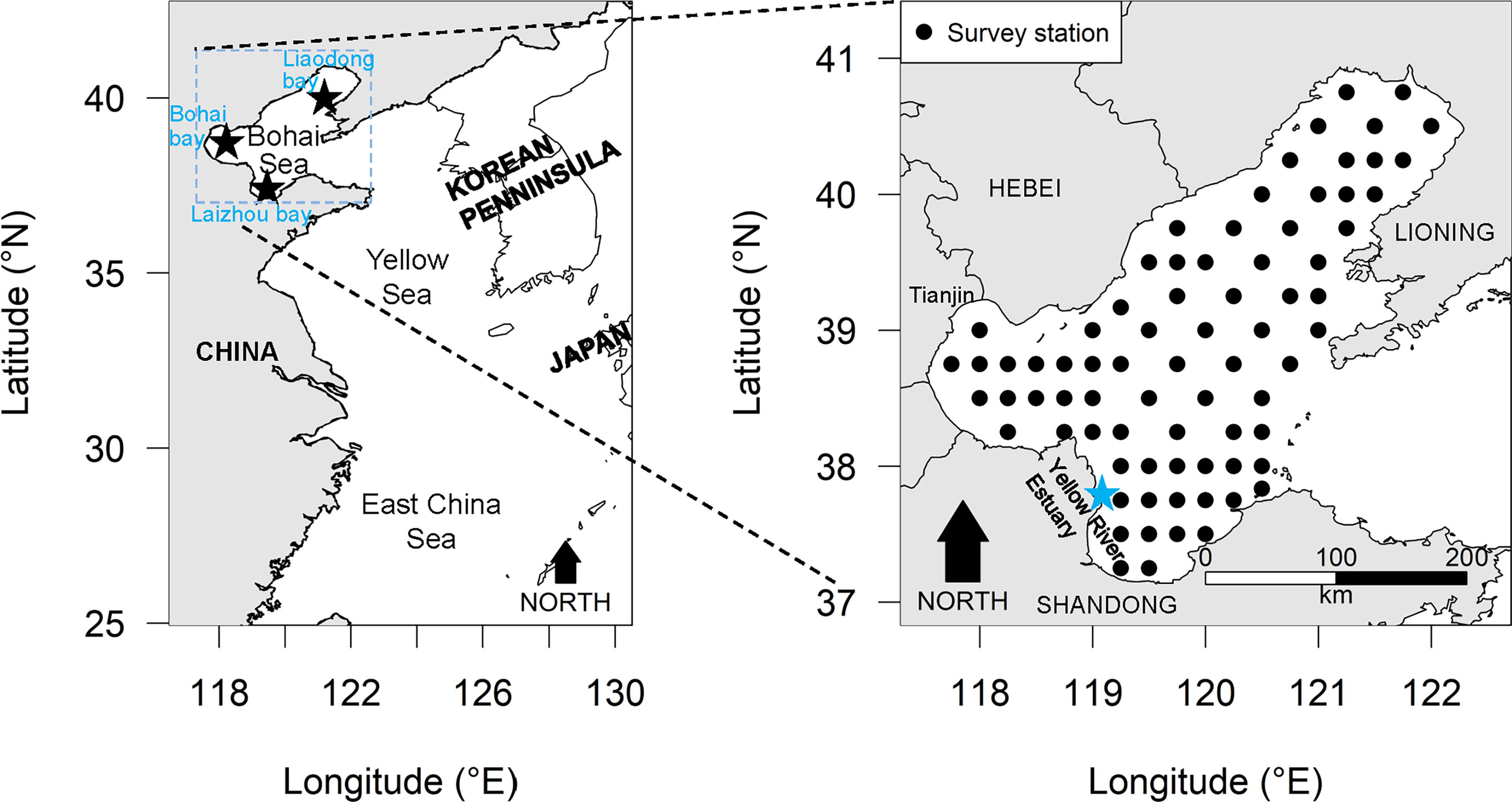
Figure 1 The locations of the Bohai Sea sampling stations where the small yellow croaker (Larimichthys polyactis) data utilized in the present study were gathered.

Material and Methods

In this study, fishery independent catch rates (kg.km^-²) of small yellow croaker from the Bohai Sea (northern Yellow Sea-Bohai Sea stock) during spring and summer from 1982–2018 were fitted using a spatio-temporal delta-Gamma model. The main objective was to identify shifts in distribution patterns indicative of range expansion or contraction of the stock in its spawning, nursery, and feeding grounds under multiple environmental stressors. Initially, we developed eight alternative spatio-temporal models of the stock for each season, constructed from combinations of explanatory variables that included the effects of sea temperature, climate index, and fishing pressure. The Akaike Information Criterion (AIC; Akaike, 1974) was used to select the most parsimonious from among the eight alternative models in each instance. We included a set of regional climate indices, representing the main modalities of changing conditions in the North Pacific Ocean shown to have important effects on fish populations in the Bohai and Yellow Seas (e. g. Liu et al., 2017). Using a pre-analysis of each season, the best climate index was selected as a model covariate, described below in more detail. Next, we used estimates from the eight models to identify the relative importance of local temperature, climate index, and fishing pressure for each season. Finally, changes in centers of gravity (COGs) i.e., centroid of stock abundance or biomass, and effective area occupied by the stock were analyzed using the model with the smallest AIC in each season, to capture the distributional shifts in geographic range of small yellow croaker in its spawning, nursery and feeding grounds and its relationship with multiple stressors. In this study, the spatially varying coefficient model (SVC, Thorson, 2019b) was used to represent the effects of annual indices (i.e., climate index and fishing pressure index) in our spatio-temporal model.

Data Used in This Study

The data for small yellow croaker in the Bohai Sea analyzed in the present study were all from scientific i.e. fishery independent, surveys using bottom trawl at fixed stations (Figure 1), conducted by the Yellow Sea Fisheries Research Institute (YSFRI). The spring (May) survey years for which records were available included 1982, 1993, 1998, 2004, 2011, 2014, and 2016–2018; Summer (August) survey years included 1982, 1992–1998, 2009–2010, 2012–2013, 2015–2018. Local commercial fishing vessels were hired as the research vessels for trawling (1-hour tows at a speed of 3 knots). Except for 2011 (mono trawl), the surveys were conducted using tandem commercial fishing vessels (pair-trawling). The power of the survey vessels before 2011, 2011 and after 2011 was 200 horsepower, 350 horsepower and 490 horsepower, respectively. Detailed information about these fishing vessels can be found in some published literature (Zhang et al., 2015; Shan and Jin, 2016; Li et al., 2018). The net mouth had a width of 22.6m, height of 6m, circumference of 109.62m, and cod-end mesh size of 20mm. Samples from all stations were identified to the level of species or lowest taxon as far as possible. Biomass was estimated as weight, abundance as number of individuals from each shot.

The environmental stressor data in this study included local sea temperature, climate index, and fishing pressure index for the period 1981–2018. Remotely-sensed sea temperature data were used because temperature data were not collected for the complete survey time series and the entire Bohai Sea area. Daily sea surface temperature (SST) data for the study area from May 1981–2018 were downloaded from the Optimum Sea Surface Temperature (OISST) Database (https://www.ncei.noaa.gov/products/optimum-interpolation-sst) of the National Centers for Environmental Information, NATIONAL OCEANIC AND ATMOSPHERIC ADMINISTRATION (NOAA). The spatial accuracy of the data is 0.25° × 0.25°, which matches the precision of our research grid. We converted the Daily SST into an estimate of mean SST (May) for each survey. Considering that the water depth of the Bohai Sea is relatively shallow, with an average of only 18.7m, and the seawater temperature is low with vertical mixing during spring producing a relatively uniform temperature throughout the water column, SST was used as a proxy for the temperature of each layer of the water column, including the bottom temperature (Jin et al., 2005; Radlinski et al., 2013). The station-measured bottom and surface temperature data obtained during the spring survey in 2017 showed a strong correlation (r = 0.98). Therefore, it is reasonable to assume that SST in spring may have a potential relationship with population dynamics of small yellow croaker in the relatively shallow waters of the Bohai Sea even though it is a benthopelagic species. In summer, SST cannot be used as a substitute for bottom temperature because the upper and lower layers of the water column are not sufficiently mixed, and the 2017 survey data only showed a weak correlation between SST and bottom temperature in August (r = 0.6). Therefore, we downloaded the bottom temperature data with coarse spatial accuracy (0.5° × 0.5°) for the study area from August 1981–2018 and interpolated them. This bottom temperature data information was available at the National Marine Data Center of China (http://mds.nmdis.org.cn/pages/dataViewDetail.html?dataSetId=81).

Pacific Decadal Oscillation (PDO, Mantua et al., 1997), North Pacific index (NPI, Trenberth and Hurrell,1994), West Pacific index (WPI, Barnston and Livezey, 1987), North Atlantic Oscillation (NAO, Hurrell, 1995; Hurrell and Deser, 2010; Hurrell et al., 2003), Northern Oscillation Index (NOI, Schwing et al., 2002), Niño 3.4 index (Trenberth, 1997), Southern Oscillation Index (SOI, Trenberth, 1984) and Arctic Oscillation index (AOI, Thompson and Wallace, 1998; Thompson and Wallace, 2001) data (downloaded from https://psl.noaa.gov/data/climateindices/list/) and their 1-year advance time series that considered the delayed/lag effect (represented by -_lag1, such as PDO_lag1.) were utilized as climatic pressure indices in the present study. These indices were downloaded for spring months (March-May), summer months (June-August), and the annual individual climatic index values for each study season (spring and summer) used in the present study were the average values of the individual indices for the seasonal month groups for each year. Oceanographic indices summarize the physical status of marine ecosystems (Grimmer, 1963; Kidson, 1975), established by many studies to have direct or indirect effects on marine fishery populations (Mantua and Hare, 2002; O’Leary et al., 2018). These climate indicators are briefly described and summarized in the appendix (Supplementary Table 1). In this study, time series of these regional indices and their respective advance time series that incorporated a 1-year lag effect were chosen as climate pressure indices because they are well recorded and updated in the Bohai Sea, and many studies have shown them to be largely associated with changes in the North Pacific marine ecosystem (Nakata and Hidaka, 2003; Overland et al., 2008; Tian et al., 2008; Shen, 2012; Tian et al., 2014; Liu et al., 2017; Yuan et al., 2017; He, 2002; Liu et al., 2021). Some of these indices have been shown to be strongly correlated with yield changes in small yellow croaker (Liu et al., 2017).

Finally, fishing mortality has been recognized as a main driver behind variation in distribution in the Bohai and Yellow Seas (Xu et al., 2003; Lin et al., 2016). No accurate commercial catch and effort data were available for the small yellow croaker stock in the Bohai Sea. Fishing power estimates were derived from records provided by the Bureau of Fisheries and Fishery Administration of Ministry of Agriculture and Rural Affairs (Ministry of Agriculture), China. The fishing power for a given year during the period 1982–2018 was obtained as the logarithm of the total engine power of the commercil fishing vessels from the Shandong, Liaoning, and Hebei provinces of China and one Chinese city (Tianjin). In this study, the total vessel power (excluding the vessels operating in the Yellow Sea) was calibrated using internal information obtained by the YSFRI from the fisheries management departments of these provinces. However, with the development of technology and the improving social economy, the number and proportion of high-powered vessels operating in the fishery are increasing, which means that the growth rate in fishing pressure is faster than that of the total fishing vessel’s power. Fishing vessel power records had been divided into three categories for the period 2003–2018 (total power above 441kW, between 45 and 440kW, and below 44kW); and into five ranges prior to 2003, but the thresholds of five ranges before 1993 differed from those during 1993–2002. Therefore, we converted the proportion of high-powered fishing vessels into a calibration coefficient for fishing capacity enhancement. The implementation of a summer fishing moratorium reduces the time available for fishing, which affects changes in fishing pressure, so we also needed to account for variations in the proportion of fishing time expended from year to year. Therefore, we used the product of fishing power × calibration coefficient for fishing capacity enhancement × proportion of fishing months for the period 1982–2018 as the fishing pressure index (FI):

$\begin{array}{ll}F{I}_y=Powe{r}_{All, y}\times (\frac{Powe{r}_{MG, y}}{Powe{r}_{All, y}}\times \frac{Maxrang{e}_{LL, y}}{Maxrang{e}_{LL, y=1}})\times (\frac{Month{s}_{a, y}}{12}),& (1)\end{array}$

Where Power_{All, y} is the total power of fishing vessels in year y; Power_{MG, y} is the total fishing vessel power in the maximum fishing vessel power group in y; Maxrange_LL,y is the lower limit of the maximum fishing vessel power grouping threshold for year y; Months_{a, y} is the number of months available for fishing in y. We also compared the performance of the two fishing pressure indicators namely the logarithm of the index FI and the logarithm of the total power of fishing vessels Power_{All, y} in the model (see the model description below) developed in this study. Our analysis showed that the logarithm of the index FI was better than the logarithm of the Power_{All, y}, so we used the former as a proxy of fishing pressure (Supplementary Table 2).

Spatio-Temporal Modeling

We developed eight alternative spatio-temporal models for the small yellow croaker stock of the Bohai Sea for the spring and summer seasons. These models variously included or excluded the effects of local temperature, fishing pressure and climate pressure indices (e.g., NPI), with the most parsimonious model chosen as the optimal one for each season based on the lowest AIC (Akaike, 1974). These models were a set of vector autoregressive spatio-temporal models, more precisely, delta-Gamma generalized linear mixed models (delta-Gamma GLMMs) with or without the option of adding a spatially varying coefficient (SVC) model, to account for spatiotemporal structures (unmeasured changes that vary over time) and spatial structure (unmeasured changes in long-term patterns, i.e., stable over time) at a fine scale (Thorson et al., 2015; Thorson, 2019a; Thorson, 2019b). The models also accounted for differences in relative fishing efficiency introduced by the different survey vessels (Thorson et al., 2015). We fitted these spatio-temporal models to the catch rate data of small yellow croaker collected during the survey in each season (spring and summer). Specifically, the following eight models comprising up to 3 covariates were fitted, M1: a model with no covariates; M2: a model with the quadratic effect of local temperature, representing a dome-shaped response to local temperatures; M3: a model with the spatially-varying effects of the individual climate indices (e.g., NPI) represented using an SVC model option (Thorson, 2019b), and which was used for pre-analysis, with the climate index in the model with the lowest AIC being selected for each season; M4: a model with the spatially-varying effect of fishing pressure; M5: a model with the quadratic effect of local temperature and the spatially-varying effect of fishing pressure; M6: a model with the quadratic effect of local temperature and the spatially-varying effect of climate index (this climate index was selected from the M3 pre-analysis); M7: a model with the spatially-varying effect of fishing pressure and the spatially-varying effect of climate index (r this climate index is selected by M3 pre-analysis); and M8: a model with the quadratic effect of local temperature, the spatially-varying effect of fishing pressure, and the spatially-varying effect of climate index (this climate index was selected from the M3 pre-analysis).

Because some of the survey catch rate data was zero-inflated, we chose the spatio-temporal delta-Gamma GLMM (Thorson et al., 2015) which comprised a binomial-GLMM and a Gamma-GLMM. This GLMM combination fitted the 0/1 (encounter/non-encounter) data and the data of the stations where small yellow croaker were caught (non-zero catch data), respectively, and multiplied the predicted values of the two parts to obtain the final biomass-density estimates (Lo et al., 1992; Grüss et al., 2019b; Han et al., 2021). In this study, the spatio-temporal delta-GLMM was employed not only to analyse spatio-temporal distribution patterns of small yellow croaker density in spring and summer, but also to identify the extent to which COGs and the effective area occupied by the stock may have shifted during 1982–2018, as described below.

Since model M8 contains the largest number of covariables (including SST, climate index and fishing pressure), its structure is described here; the structures of the M1-M7 models are similar. The binomial-GLMM with a logit link function and linear predictors was used to estimate the probability of small yellow croaker being caught (encounter) p_i at sampling station s(i).The binomial-GLMM included two Gaussian Markov random fields which represent respectively the spatial variation and the spatio-temporal variation in encounter probability:

$\begin{array}{ll}{p}_i=logi{t}^{-1}\left({\beta }_{t\left(i\right)}^{\left(p\right)}+r_{V\left(i\right),t\left(i\right)}^{\left(p\right)}+{\omega }_{s\left(i\right)}^{\left(p\right)}+{ϵ}_{s\left(i\right),t\left(i\right)}^{\left(p\right)}+{\gamma }_{t\left(i\right),1}^{\left(p\right)}{T}_{s\left(i\right),t\left(i\right)}^{\left(p\right)}+{\gamma }_{t\left(i\right),2}^{\left(p\right)}{T}_{s\left(i\right),t\left(i\right)}^{2\left(p\right)}+{\xi }_{s\left(i\right),t\left(i\right),1}^{\left(p\right)}+{\xi }_{s\left(i\right),t\left(i\right), 2}^{\left(p\right)}\right)& (2)\end{array}$

where ${\beta }_{t\left(i\right)}^{\left(p\right)}$ is the intercept for year t(i) in which sample i; $r_{\left(V\left(i\right),t\left(i\right)\right)}^{\left(p\right)}$ is the relative fishing efficiency for the v^th survey vessel at site s(i)in year t(i); ${\omega }_{s\left(i\right)}^{\left(p\right)}$ is the spatially correlated variability in encounter probability at the station s(i) where sample i; ${ϵ}_{ s\left(i\right)t\left(i\right)}^{\left(p\right)}$ is the spatially correlated variability in encounter probability at station s(i) in year t(i); ${\gamma }_{t\left(i\right),1}^{\left(p\right)}{T}_{s\left(i\right),t\left(i\right)}^{\left(p\right)}$ is the linear effect of local temperature on encounter probability at station s(i) in year t(i); ${\gamma }_{t\left(i\right),2}^{\left(p\right)}{T}_{s\left(i\right),t\left(i\right)}^{2\left(p\right)}$ is the quadratic effect of local temperature on encounter probability at station s(i) in year t(i); ${\xi }_{s\left(i\right),t\left(i\right),1}^{\left(p\right)}$ is the spatially-varying effect of the climate indices (e.g., NPI) on encounter probability at s(i) in t(i); and ${\xi }_{s\left(i\right),t\left(i\right), 2}^{\left(p\right)}$ is the spatially-varying effect of fishing pressure on encounter probability at station s(i) in year t(i). Prior to being used in the models, both the T and T² covariates were standardized to have a mean of zero and a variance of one; this transformation implied that ${\gamma }_1^{\left(p\right)}{T}^{\left(p\right)}$ and ${\gamma }_2^{\left(p\right)}{T}^{2\left(p\right)}$ had a standard deviation equal to ${\gamma }_1^{\left(p\right)}$ and ${\gamma }_2^{\left(p\right)}$, respectively (Thorson, 2015; Grüss et al., 2020a; Han et al., 2021).

The ${\beta }_t^{\left(p\right)}$ ,${\gamma }_{t,1}^{\left(p\right)}{T}_{\left(t\right)}^{\left(p\right)}$ and ${\gamma }_{t,2}^{\left(p\right)}{T}_{t\left(i\right)}^{2\left(p\right)}$ are fixed effects. The $r_{V,t}^{\left(p\right)}$ ω^(p) ${ϵ}_t^{\left(p\right)}$ ,${\xi }_{t,1}^{\left(p\right)}$ and ${\xi }_{t,2}^{\left(p\right)}$, are random effects and were assumed to follow a multivariate normal distribution and, in the case of the ${ϵ}_t^{\left(p\right)}$, temporal variation was expected to conform to a random-walk process (Thorson et al., 2016a) in time to ensure that year intervals or/and stations that have not been sampled do not present mean-reversion:

$\begin{array}{ll}\begin{array}{c}{r}_v^{\left(p\right)}~N\left(0,{\sigma }_{pr}^2\right)\\ {\omega }^{\left(p\right)}~MVN\left(0,{\sigma }_{p\omega }^2\text{R}\left(\kappa \right)\right)\\ {ϵ}_t^{\left(p\right)}~MVN\left({ϵ}_{t-1}^{\left(p\right)},{\sigma }_{pϵ}^2\text{R}\left(\kappa \right)\right)\\ {\xi }_{t,1}^{\left(p\right)}~MVN\left(0,{\sigma }_{p\xi ,1}^2{\theta }_{s,1}{P}_{t,1}\right)\\ {\xi }_{t,2}^{\left(p\right)}~MVN\left(0,{\sigma }_{p\xi ,2}^2{\theta }_{s,2}{P}_{t,2}\right),\end{array}& (3)\end{array}$

Where ${\sigma }_{pr}^2$ is the variance of vessel effects (encounters);R(k) is the correlation among stations as a function of decorrelation distance k;${\sigma }_{p\omega }^2$ and ${\sigma }_{pϵ}^2$ are the pointwise variance of ω^(p) theand ${ϵ}_t^{\left(p\right)}$, respectively; P_t,1 is the climate indices (e.g., NPI) and θ_s,1P_t,1 is the climate indices (e.g., NPI) effect; and ${\sigma }_{p\xi , 1}^2$ is the pointwise variance of the climate indices (e.g., NPI) effect.P_t,2 is the fishing pressure; and θ_s,2P_t,2 is the effect of fishing pressure and ${\sigma }_{p\xi , 2}^2$ is its pointwise variance. The calculation method of the R terms can be found in Thorson et al. (2015).

Similarly, the non-zero catch rate of small yellow croaker r_i at station s_i was estimated by the Gamma components (has a log link function) and linear predictors, including two Gaussian Markov random fields accounting for spatial variation and spatio-temporal variation in non-zero catch rate, respectively:

$\begin{array}{ll}{r}_i=exp\left({\beta }_{t\left(i\right)}^{\left(r\right)}+r_{V\left(i\right),t\left(i\right)}^{\left(r\right)}+{\omega }_{s\left(i\right)}^{\left(r\right)}+{ϵ}_{s\left(i\right),t\left(i\right)}^{\left(r\right)}+{\gamma }_{t\left(i\right),1}^{\left(r\right)}{T}_{s\left(i\right),t\left(i\right)}^{\left(r\right)}+{\gamma }_{t\left(i\right),2}^{\left(r\right)}{T}_{s\left(i\right),t\left(i\right)}^{2\left(r\right)}+{\xi }_{s\left(i\right),t\left(i\right),1}^{\left(r\right)}+{\xi }_{s\left(i\right),t\left(i\right), 2}^{\left(r\right)}\right),& (4)\end{array}$

where most of the parameters of Eq. (4) have the same meaning as the parameters of Eq. (2), except that they apply to log-catch rate.

To improve computational efficiency, following Han et al. (2021), 100 “knots” n_j = 100 were specified to approximate all the ω^(p), ω^(r), ${ϵ}_t^{\left(p\right)}$,and ${ϵ}_t^{\left(r\right)}$, over a fixed spatial domain Ω, so that the value of each variation term is tracked at each knot (Shelton et al., 2014; Thorson et al., 2015). These knots were distributed over a grid (Figure 2) developed for this study. All ω^(p), ω^(r), ${ϵ}_t^{\left(p\right)}$, ${ϵ}_t^{\left(r\right)}$ were tracked at each knot by the model, and the value of each term at a prediction grid cell is interpolated from the value of three knots surrounding that grid cell (see Grüss et al., 2020a; Grüss et al., 2020b; Grüss et al., 2020c). The 100 knots provided a compromise between the estimation accuracy and run time of the GLMM model. As the number of knots increased, the parameter estimates and predictions became similar.

FIGURE 2

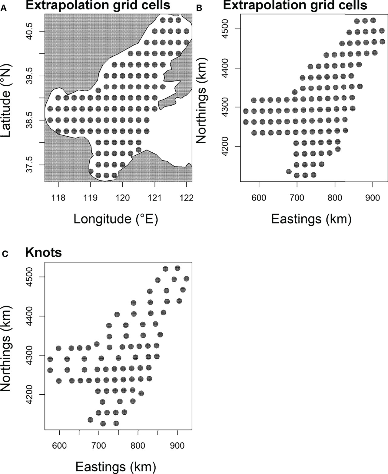
Figure 2 The barycenter of 116 extrapolation grid cells (15× 15 arc-minutes) and of “knots” of the Bohai Sea in the present study. This barycenters of grid are depicted in (A, B). To improve computational efficiency, 100 “knots” (C) were assigned to approximate the spatial and spatio-temporal variation components of the model developed for the present work.

According to the results obtained by multiplying the predicted values of the binomial-GLMM and the predicted values of the Gamma-GLMM, we mapped the biomass-density of small yellow croaker in spring and summer separately on the Bohai Sea prediction grid. Next, the biomass of the small yellow croaker stock in year t, ${\widehat{B}}_t$ was estimated, as:

$\begin{array}{ll}{\widehat{B}}_t={\displaystyle \sum _{j=1}^{n_j}{A}_j{\widehat{p}}_{j,t}{\widehat{r}}_{j,t}}={\displaystyle {\sum }_{j=1}^{n_j}\begin{array}{c}{A}_{j}logi{t}^{-1}\left({\widehat{B}}_t^{\left(p\right)}+{\widehat{r}}_{V,t}^{\left(p\right)}+{\widehat{\omega }}_j^{\left(p\right)}+{\widehat{ϵ}}_{\text{'}j,t}^{\left(p\right)}+{\widehat{\gamma }}_{t,2}^{\left(p\right)}{T}_{j,t}^{2\left(p\right)}+{\widehat{\xi }}_{j,t, 1}^{\left(p\right)}+{\widehat{\xi }}_{j,t, 2}^{\left(p\right)}\right)\\ exp\left({\widehat{\beta }}_t^{\left(r\right)}+{\widehat{r}}_{V,t}^{\left(r\right)}+{\widehat{\omega }}_j^{\left(r\right)}+{\widehat{ϵ}}_{j,t}^{\left(r\right)}+{\widehat{\gamma }}_{t,1}^{\left(r\right)}{T}_{j,t}^{\left(r\right)}+{\widehat{\gamma }}_{t,2}^{\left(r\right)}{T}_{j,t}^{2\left(r\right)}+{\widehat{\xi }}_{j,t, 1}^{\left(r\right)}+{\widehat{\xi }}_{j,t, 2}^{\left(r\right)}\right)\end{array}}& (5)\end{array}$

where A_j is the surface area of knot j (in km²); ${\widehat{\beta }}_t^{\left(p\right)}$, ${\widehat{\gamma }}_{\text{'}t,1}^{\left(p\right)}$ , ${\widehat{\gamma }}_{t,2}^{\left(p\right)}$, ${\widehat{\beta }}_t^{\left(r\right)}$ and ${\widehat{\gamma }}_{t,1}^{\left(r\right)}$ are fixed effects estimated via maximum likelihood; and ${\widehat{r}}_{V,t}^{\left(p\right)}$ ,${\widehat{ϵ}}_{j,t}^{\left(p\right)}$, ${\widehat{\omega }}_j^{\left(p\right)}$, ${\widehat{\xi }}_{j,t}^{\left(p\right)}$, ${\widehat{r}}_{V,t}^{\left(r\right)}$, ${\widehat{ϵ}}_{j,t}^{\left(r\right)}$, ${\widehat{\omega }}_j^{\left(r\right)}$, ${\widehat{\xi }}_{j,t,1}^{\left(r\right)}$ and ${\widehat{\xi }}_{j,t,2}^{\left(r\right)}$ are random effects (Thorson et al., 2015).

To measure the shifts in spatial distribution of the stock over time, we calculated its annual COGs in spring and summer during 1982–2018. The eastward COG, X_t, was calculated by (Thorson et al., 2016a; Thorson et al., 2016b; Thorson and Barnett, 2017):

$\begin{array}{ll}{X}_t={\displaystyle \sum _{j=1}^{nj}{x}_j\frac{A_j{\widehat{p}}_{j,t}{\widehat{r}}_{j,t}}{{\widehat{B}}_t}}& (6)\end{array}$

where x_j is the easting value (in km) in knot j. The northward COG, Y_t, can be shown in a similar way, except that x_j is replaced with y_j ,the northing value (in km) in knot j, in Eq. (6).

To determine the annual range expansion/contraction of the stock in spring and summer, we estimated the annual effective area occupied by the stock during 1982–2018. Effective area occupied is shown by the ratio of predicted biomass (Eq. (5)) over average density, D_t, which is calculated by (Thorson et al., 2016a; Thorson et al., 2016b):

$\begin{array}{ll}{D}_t={\displaystyle {\sum }_{j=1}^{n_j}{\widehat{p}}_{j,t}{\widehat{r}}_{j,t}\frac{A_j{\widehat{p}}_{j,t}{\widehat{r}}_{j,t}}{{\widehat{B}}_t}}.& (7)\end{array}$

The models were implemented using the “VAST” package (https://github.com/James-Thorson-NOAA/VAST Thorson, 2019a) within the R statistical software environment on Windows (R Core Team, 2021). The estimation of fixed effects, random effects and their standard deviations, as well as the standard deviations of derived quantities were mainly calculated by the Laplace approximation, the stochastic partial differential equation method (Lindgren et al., 2011), and the generalized delta method (Kass and Steffey, 1989) implemented using the R package “TMB” (Kristensen et al., 2016), and the bias-correction estimator developed in Thorson and Kristensen (2016). Their detailed computational descriptions are documented in Thorson et al. (2015) and Thorson (2019a). The convergence test of the spatio-temporal model comprised two parts: (1) the gradient of marginal logarithmic likelihood of all fixed effects should be less than 0.0001; and (2) the Hessian matrix of the second derivative of negative logarithmic likelihood must be positive definite. In addition, the “VAST” package also has a set of diagnostics, which can further confirm whether the spatio-temporal models were reasonable, i.e., that (1) the observed encounter frequencies were within the 95% prediction interval of the predicted encounter probability; (2) the diagnostics for the positive-catch-rate component using a q-q plot showed the residuals lay along the one-to-one line; and (3) mapping Pearson residuals for encounter-probability and positive catch rates of the small yellow croaker stock showed that there were no visible patterns in the Bohai Sea.

Understanding the Relative Importance of Three Stressor Covariables in Explaining Distribution Patterns of Small Yellow Croaker

We employed the eight models (with various combinations of the effects of local temperature, climate indices, and fishing pressure) for each season, and applied the method used in Thorson (2015) to analyze the relative importance of multiple stressors explaining the probability patterns of encounter and non-zero density (estimated by the delta-Gamma GLMM) of small yellow croaker in the Bohai Sea in spring and summer, respectively. Based on the method used in Thorson (2015), we compared the variances of the spatio-temporal variations (the sum of the spatial variation term and of the spatio-temporal variation terms) in the probability of encounters and non-zero density for the eight alternative delta-Gamma GLMMs for each season in this study to determine whether some reduction of the variances caused by local temperature and/or climate index and/or fishing pressure covariable(s) was/were included in a model. The desired goal of the inclusion of covariables in the models was to minimize the spatio-temporal variability, which represents the latent (unmeasured) variation in the encounter probability or non-zero density probability of the stock (Thorson et al., 2015; Han et al., 2021).

Trend Analysis of Local Temperature, Climate Index and Fishing Pressure Index Time Series

We also performed trend analyses of the local temperature, climate index and fishing pressure index time series in spring and summer as an aid for interpreting the estimates of the most parsimonious (i.e., the smallest AIC value) spatiotemporal model. These trend analyses were performed by the regime shift detection method based on a sequential t-test to detect possible regime shifts, which requires the data to be processed with “pre-whitening” prior to use (Rodionov, 2004; Rodionov and Overland, 2005; Rodionov, 2006).

Results

The Relative Importance of the Fishing Pressure, SST and the Climate Index in Explaining Distribution Patterns

In this study, eight models (delta-Gamma GLMMs) for the small yellow croaker stock in the Bohai Sea during spring and summer, were developed (M1-M8) by incorporating different combinations of the effects of fishing pressure, local temperature, and climate indices (e.g., NPI). All the models satisfied tests of convergence and diagnostic requirements (The diagnostic results of the AIC-selected models are shown in Supplementary Figure 1, 2). Comparisons among the M1-M8 models for each season allowed us to identify the relative importance of fishing pressure, local temperature and the climate indices (e.g., NPI) in explaining the probability patterns of encounter and density of the stock during each specific season. The results from the pre-analysis of M3 in spring indicated that M3 with the NPI covariable had a smaller AIC value than M3 with the other climate index covariables. In spring, we found that when interpreting the probability pattern of encounter, the variances of M1-M8 were all equal to or extremely close to 0, and NPI and fishing pressure were relatively more important than local temperature (Table 1). Including NPI or fishing pressure in the model, the variance of spatio-temporal variation of encounter probability remained unchanged relative to M1, while including local temperature in the model caused a negligible increase of the variance. Conversely, we found that SST was more important than NPI and fishing pressure in interpreting the non-zero density pattern during spring (Table 1). The inclusion of local temperature in the model caused a large decrease in the spatio-temporal variance in density, whereas the inclusion of NPI or fishing pressure caused a moderate increase in the variance.

TABLE 1

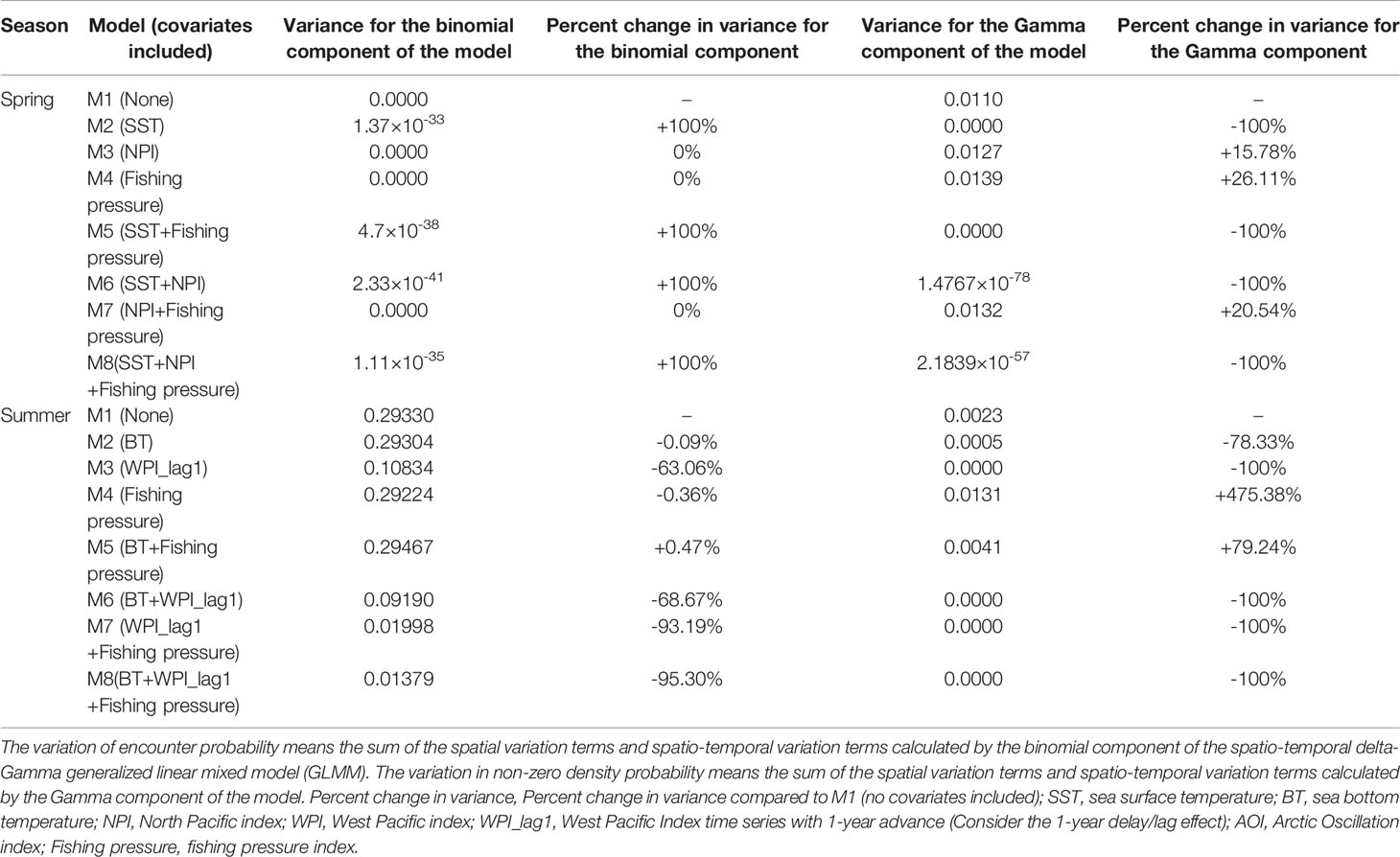
Table 1 The variances of the spatio-temporal variations of encounter probability and non-zero density probability calculated by the eight models developed in spring and summer in the present study (M1-M8).

The results of pre-analysis of M3 in summer indicated that M3 with the WPI_lag1 (WPI lagged by 1-year) covariable had a smaller AIC value than M3 with other climate index covariables. We found that WPI_lag1 was more important than local temperature and fishing pressure when interpreting the probability pattern of encounter in summer (Table 1). Including WPI_lag1 in the model, the spatio-temporal variation in encounter probability showed a large decrease relative to M1, while including local temperature or fishing pressure in the model caused a negligible or small decrease in the variance. Moreover, the WPI_lag1was more important than local temperature and fishing pressure in explaining the probability patterns of density; and local temperature was more important than fishing pressure (Table 1). Including the WPI_lag1 or local temperature in the model caused a large decrease in spatio-temporal variation in density probability, whereas including fishing pressure in the model caused a large increase in the variance.

Change Patterns of Spatiotemporal Distribution and Range of Small Yellow Croaker in the Bohai Sea

In spring, the AIC value of the spatial-temporal model with the quadratic effect of local temperature, the spatially-varying effect of NPI and the spatially-varying effect of fishing pressure was the lowest (Table 2). Model M8, selected by AIC, predicted that the biomass-densities of small yellow croaker in the middle and southern area of Liaodong Bay (39°00′-40° 20′N, 120°00′-121° 37.5′E) was the highest in the Bohai Sea during 1982–2018 (Figure 3). Other hotspots (i.e. locations with the highest densities) for the stock were in the central Bohai Sea (38°15′-39°00′N, 119°00′-121°00 ′E). The M8 also predicted the biomass of small yellow croaker in spring would have dropped sharply in general over the period of 1982–2018 (decreasing significantly from 1982 to 1998; mostly increasing from 1998 to 2011; declining sharply from 2011 to 2014; and increasing moderately between 2014 and 2018), leading to large distribution changes of the stock in their spawning ground during the whole study period (Figure 3 and Supplementary Figure 3). The annual intercept of the gamma component (i.e., the ${\beta }_t^{\left(r\right)}$ term in equation (4)) reflected the biomass change, which also declined markedly in 1982–1998; increased largely in 1998–2011; decreased sharply in 2011–2014; and increased modestly in 2014–2018. Since 2011, biomass density in spring decreased significantly, accompanied by the disappearance of the hotspot area (Figure 3 and Supplementary Figure 3). This disappearance/contraction was more pronounced in the western (Bohai Bay) and southern (Laizhou Bay) areas of the Bohai Sea than in the mid-eastern regions. After 2011, the density of the stock in the Yellow River Estuary and the southwest areas of Laizhou Bay was close to zero and showed a slow recovery; especially in the southwest areas of Laizhou Bay, which had a negligible recovery in 2017–2018. In 2018, the central area of Liaodong Bay close to the Liaodong Peninsula remained the only density hotspot in the Bohai Sea (Supplementary Figure 3).

TABLE 2

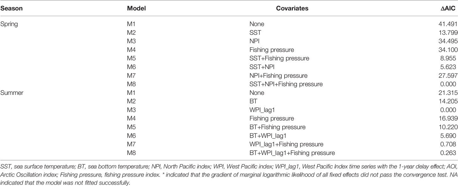
Table 2 Model selection based on Akaike’s information criterion (AIC) for the eight alternative spatio-temporal delta-Gamma models in spring and summer, respectively fitted in the present study.

FIGURE 3

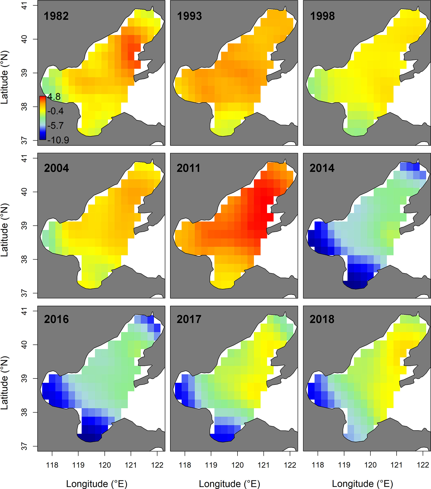
Figure 3 Spatio-temporal distribution of log-density for the small yellow croaker stock of the Bohai Sea in spring of 1982−2018, predicted by the Akaike’s information criterion (AIC)-selected model developed for the stock. The color legend with units ln(kg.km^-2) is provided in the first panel and has. Only projections for years where sampling for the stock were available (i.e., 1982, 1993, 1998, 2004. 2011, 2014 and 2016–2018) are presented.

In summer, the spatio-temporal model (M3) with the spatially-varying effect of WPI_lag1 had the lowest AIC (Table 2). This AIC-selected model M3 predicted that the hotspots of small yellow croaker in the Bohai Sea would be found in the area near the line connecting the junction of Bohai Bay and Laizhou Bay to the northern area of Liaodong Bay in the summer of 1982–2018 (Figure 4). We also found that the predicted hotspots moved left (west) or right (east) along the diagonal between years. M3 also predicted that the biomass decreased markedly in general in the summer between 1982 and 2018, leading to substantial distribution changes of the stock in their nursery and feeding grounds over the entire study period (Figure 4 and Supplementary Figure 4). The ${\beta }_t^{\left(r\right)}$ terms also showed a significant overall decline during 1982–2018. Since 2009, the density of the stock in the Bohai Sea in summer decreased significantly, accompanied by shrinkage of the high-density areas (Figure 4 and Supplementary Figure 4). The shrinkage was more obvious in Bohai Bay, the eastern area of Laizhou Bay and the central area of the Bohai Sea than in Liaodong Bay. In 2012 and 2016, the density in the Yellow River estuary remained relatively high in the area south of 39°N. By the second half of the 2010s, except for 2016, only the Liaodong Bay area retained a biomass hotspot for the stock (Supplementary Figure 4). Combining the trends of the stock biomass density in the Bohai Sea in the two seasons, we found that the biomass: (1) increased extremely slowly in the early 1980s to early 1990s; (2) subsequently decreased significantly during the early 1990s to late 1990s; (3) increased again largely in the early 2000s to late 2000s; (4) then decreased sharply in the early 2010s to mid-2010s; and finally (5) exhibited an extremely slow recovery trend after 2017.

FIGURE 4

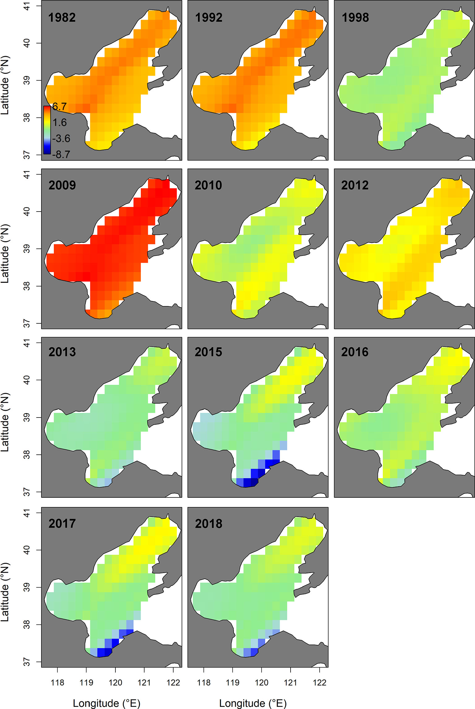
Figure 4 Spatio-temporal distribution of log-density for the stock of the Bohai Sea in summer of 1982−2018, predicted by the AIC-selected model. The color legend with units ln(kg.km^-2) is provided in the first panel. Only projections for the years where sampling for the stock were available (i.e., 1982, 1992, 1998, 2009-2010, 2012-2013 and 2015–2018) are presented.

In spring, the COGs predicted by the AIC-selected M8 suggested that the COG of the stock had moved southward and westward in spring of 1982–1993, and then northward and eastward in spring between 1993 and 2018 (Figure 5). Over the period 1982–2018, changes in both the COGs in spring were non-significant (both p > 0.05, a two-sided Wald test was used for all significance tests). However, the spring variations in eastward and northward COGs during 1993–2018 were significant (p=0.015 and 0.034, respectively). In summer, the COGs estimated by the AIC-selected M3 showed that the COG variation trend was relatively stable in the summer of 1982–2009; and then the COG moved largely to the north and east over the period 2009–2018 (Figure 5). Between 1982 and 2018, eastward changes in the COG in summer (i.e., the large move of the COG of the stock towards the east of Bohai Sea) were statistically significant (p = 0.0004, a two-sided Wald test was used for all significance tests). In addition, the northward COG changes of small yellow croaker in summer (i.e., the large move of the COG of the stock towards the north of Bohai Sea) were also significant (p = 0.0024) from 1982 to 2018.

FIGURE 5

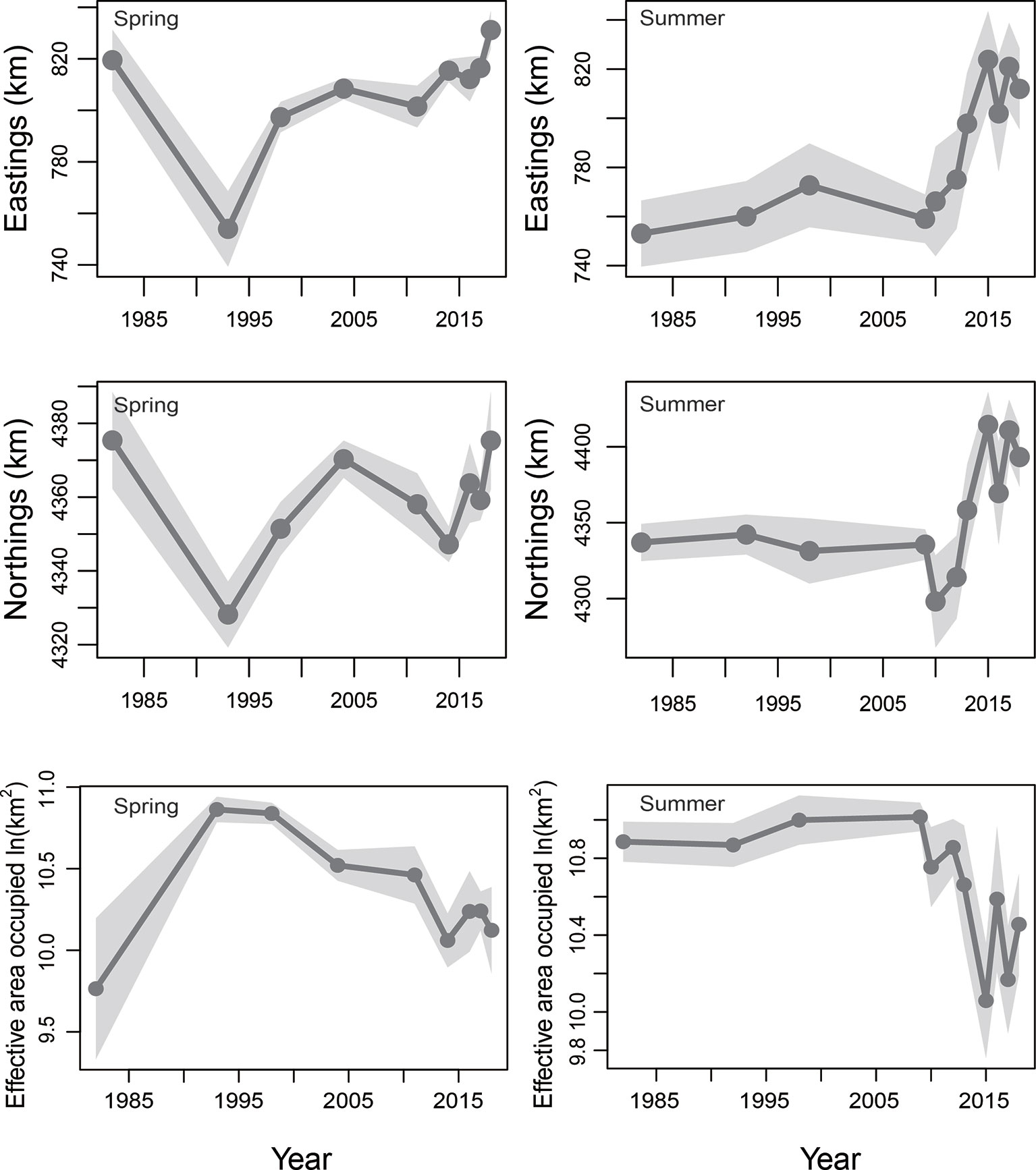
Figure 5 Eastward center of and northward center of gravity (COG; in km) and effective area occupied for the stock in spring and summer of 1982−2018, predicted by the AIC-selected model. The 95% confidence intervals are represented as shaded areas. Only projections for the years where sampling for the stock were available (i.e., 1982, 1993, 1998, 2004. 2011, 2014 and 2016–2018 for spring; 1982, 1992, 1998, 2009-2010, 2012-2013 and 2015–2018 for summer) are given.

In spring, the effective area occupied of the stock predicted by the M8 indicated that range contraction had occurred during the study period from 1993 to 2018 (Figure 5). However, from 1982 to 2018, the effective area occupied by the stock in spring did not change significantly (p >0.05). In summer, the effective area occupied in the Bohai Sea predicted by the M3 showed that the range of the stock was reduced (Figure 5). Statistically, the change in effective area occupied by the stock in summer from 1982 to 2018 was also significant (p = 0.046).

Trend Analysis of Local Temperature, Climate Index and Fishing Pressure Index Time Series

From 1982 to 2018, the local temperature anomalies in May showed an oscillatory rising trend, and the mean SST difference between the former and the latter five years was 1.96℃. The SST time series showed that regime shifts in temperature occurred in 1995/1996 and 2013/2014 respectively (Figure 6A), mirroring the switch from a southward to a northward shift of the small yellow croaker COG in spring in 1993 and in 2014 respectively. The time series indicated (Figure 6B) that there were no regime shifts in the spring NPI during the period 1981–2018. The change in trend of the cumulative sum of NPI anomalies in spring was, to a certain extent, similar to the trend in the COG in spring.

FIGURE 6

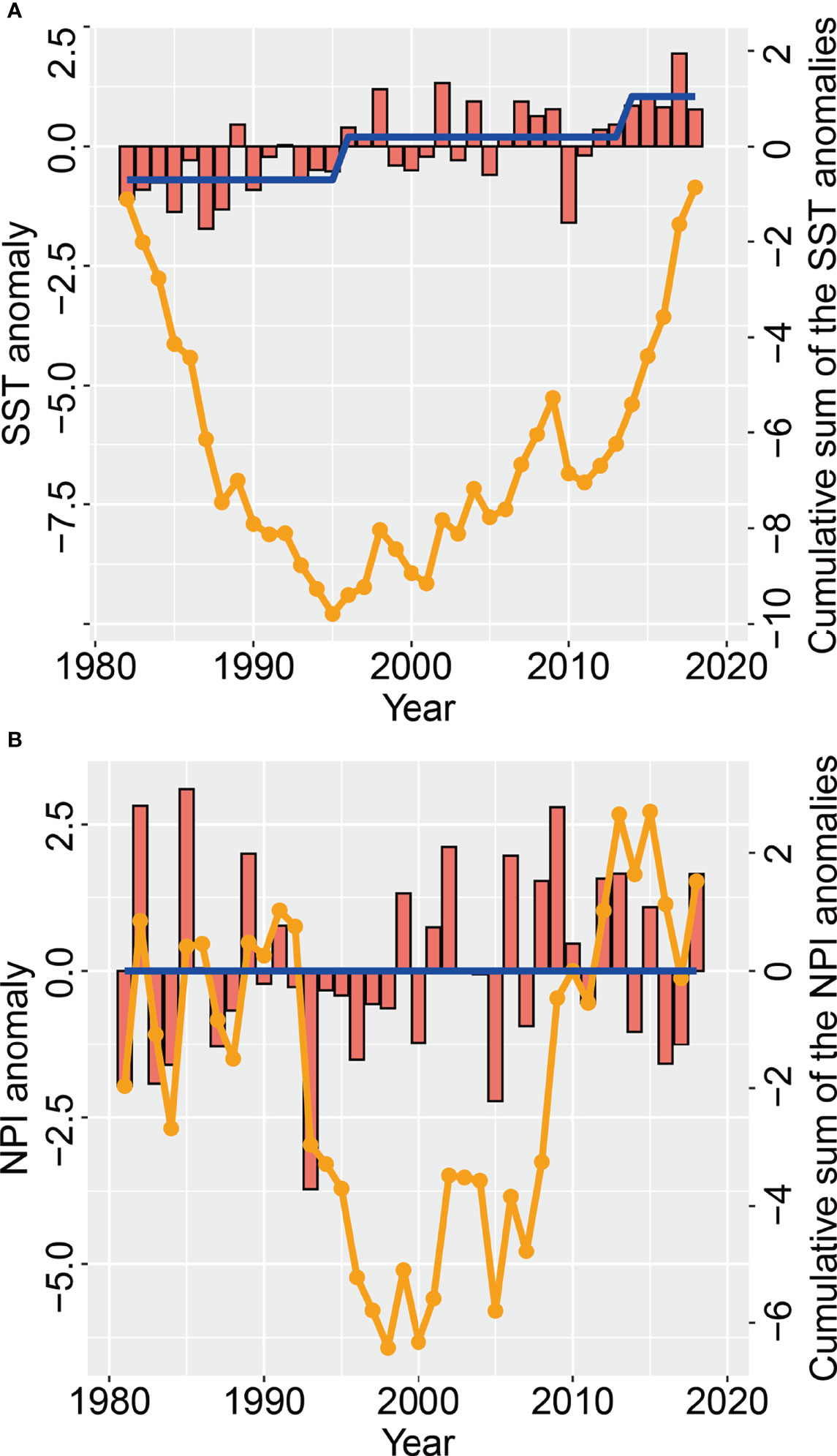
Figure 6 Changes in (A) May sea surface temperature (red bars) anomalies (SSTA) and (B) spring North Pacific index (NPI) anomalies (red bars), as well as the cumulative sum of the NPI and SST anomalies (orange line), in the Bohai Sea over the period 1981−2018 The regime shift (blue line) in the NPI and SST is also given.

In summer, there was a large seasonal oscillation in local temperature anomalies during August of each year (Figure 7A). The overall trend of local temperature was stable from 1982 to 2008, whereas it increased greatly from 2008 to 2018. This obviously reflected the trend of the COG and effective area occupied of the stock in summer. Local temperature time series showed that a regime shift of the SST occurred in 2008/2009 (Figure 7A). This corresponded to the large increase in density and change in distribution in 2009. The WPI time series indicated that WPI underwent regime shifts in 2001/2002 and 2017/2018 (Figure 7B). The change in pattern of positive/negative WPI anomalies in summer between 1981 and 2018 correlated with the change in the summer pattern of biomass density.

FIGURE 7

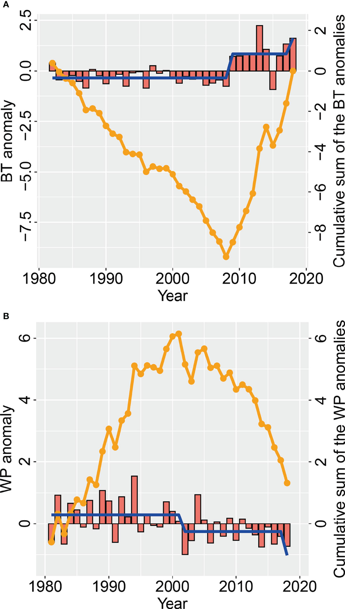
Figure 7 Changes in (A) August bottom temperature (red bars) anomalies (BTA) and (B) summer West Pacific index (WPI) anomalies (red bars), as well as the cumulative sum of the BT and WPI anomalies (orange line), in the Bohai Sea over the period 1981−2018. The regime shift (blue line) in the WPI and BT is also given.

The fishing pressure proxy rose sharply from 1982 to 1994; moderately increased during 1994–2002; fell sharply from 2002 to 2009; and increased rapidly and substantially again from 2009 to 2015; then subsequently declined somewhat to remain at relatively stable but high level thereafter (Figure 8).

FIGURE 8

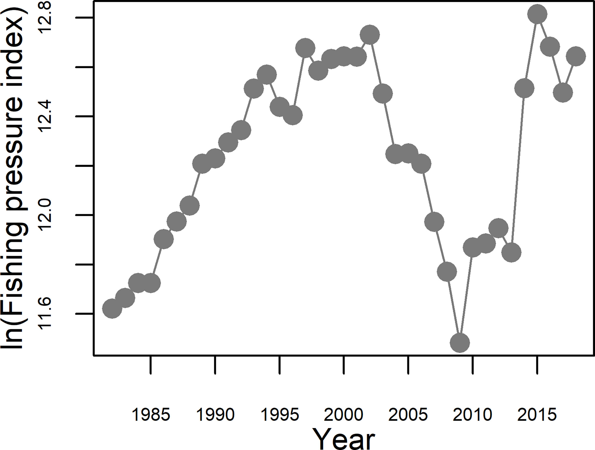
Figure 8 Changes in the proxy of fishing pressure (in ln(Fishing pressure index)) in the Bohai Sea during the period 1982−2018.

Discussion

To understand its ecological response to multiple stressors during the spawning and nursery phases of its life history, we developed a spatio-temporal model for the small yellow croaker’s populations in the Bohai Sea in spring and summer during 1982–2018. Ours is the first spatio-temporal implementation of the SVC model to determine the effects of annual indices (climate index and fishing pressure index) in the Bohai Sea. Many studies have established that spatio-temporal models which account for both spatial and spatio-temporal variation can produce more accurate estimates, thereby providing increased reliability in the scientific basis for decision-making about how best to manage marine ecosystems, their dependent fish populations, and the fisheries those populations sustain (Rassweiler et al., 2014; Thorson et al., 2015; Grüss et al., 2019b; Han et al., 2019; Thorson, 2019a; Thorson, 2019b; Han et al., 2021).

In the spatio-temporal model we developed, spatial variation refers to variation in biomass density that for the small yellow croaker in the Bohai Sea is assumed to remain constant over time. Spatio-temporal variation refers to the interannual variation in biomass density of the stock. Spatial variation and spatio-temporal variation represent, respectively, the fundamental ecological niche of the stock in the Bohai Sea and the response of the stock to the unmeasured environment stress (Grüss et al., 2017; Thorson, 2019a). Spatio-temporal models can also be used to obtain information on the stressors that cause ecological responses in fish populations and to analyze the relative magnitude of the effects of these stressors (i.e., analyzing the relative importance of the covariates) by including covariates to improve the proportion of response variation explained by a model (Thorson, 2015; Grüss et al., 2020a; Han et al., 2021). Based on these characteristics of the spatio-temporal model, this study identified multiple pressure factors influencing the population dynamics of small yellow croaker during spawning, nursery and feeding phases of their life history in the Bohai Sea.

The model results in spring and summer were expected to accord with those from a study in the East Bering Sea (Thorson, 2019b), which showed that the use of SVC models, including temperature or/and annual index (cold pool), produced more parsimonious models that better described the stock being modeled. The relationship between fishing pressure and local sea temperature with the distribution of small yellow croaker in summer was not as great as that in spring. We suspect that implementation of the summer fishing moratorium system meant that the stock dynamics during summer was not directly affected by fishing. Han et al. (2021) argued that the inclusion of local covariables and/or annual index in a similar model would not be appropriate to describe the stock being modeled in many regions; and the study of Ducharme-Barth et al. (2022) also adds a supporting case for this view. The present study supports and further develops the idea that such regions are not static, and that the inclusion of local or/and distant regional covariates in spatio-temporal models varies greatly in its suitability for describing the modeled stock in different seasons.

Insights about the spawning grounds and reproductive environment of the Bohai Sea stock of small yellow croaker in this study were predominantly consistent with those from previous studies conducted during the 1950s–1980s (Feng and Yang, 1955; Liu et al., 1990), with some additional points. Previous studies indicated that small yellow croaker entered the Bohai Sea from the Yellow Sea and divided into two routes in late April: the north route entered Liaodong Bay in mid-May; the south route continued to branch, one branch reached the spawning grounds of the Yellow Estuary of Laizhou Bay in early May, and the other branch reached the northern area of Bohai Bay (38°30’N-39°00’N, 118°00’E-118°30’E) in mid-May. Our results showed that even in mid to late May, a significant percentage of the stock remained distributed in the central Bohai Sea. Our model results also indicated that the range of spawning grounds in Bohai Bay was larger than determined in previous studies, and mainly concentrated in the northwestern area of Bohai Bay; and that in Laizhou Bay, in addition to the area around the Yellow River estuary, the stock was also distributed in the southern area of Laizhou Bay during the spawning period. The spawning grounds are crucial for replenishing the populations in the entire Yellow Sea Large Marine Ecosystem, because they attract many spawning adults (Jin et al., 2005). Our model results imply that there is a need to take more measures to focus on protecting the spawning grounds in Bohai and Laizhou Bays. Therefore, this study provides fundamental support for marine spatial planning to ensure spawning grounds are sufficiently protected to maintain sustainable fisheries.

Our model indicated that the main feeding grounds (predicted hotspots) were in the area near the line connecting the junction of Bohai Bay and Laizhou Bay to the northern area of Liaodong Bay in summer (August). This location was consistent with the main distribution area of the August fishery yield of the stock in the Bohai Sea observed during 1971–1972 (Xu and Chen, 2009, Figure 2 of the paper). However, the common feeding ground in Laizhou and Bohai Bays differed from what was identified in a previous study by Lin (1991), which determined that the common feeding ground of the stocks in Laizhou and Bohai Bays was located in the nearshore waters of Bohai Bay in northwestern Shandong Province.

In summer, M3 indicated a statistically significant shift to the northeast and range contraction of the stock in their feeding and nursery grounds over the period 2009–2018. This finding mirrored a decrease in the recruitment capacity of small yellow croaker in the Bohai Sea after 2009, with its northeastern area declining relatively slower than the other regions of the Bohai Sea. As per the spring results, this finding also implied a decline in ecological function (cradle) in Bohai and Laizhou Bays in recent years and the need to focus on restoring their functionality.

Next, we discuss the role of local temperature, climate index and fishing pressure in driving the decadal spatio-temporal patterns of the stock in its spawning, nursery and feeding grounds in the Bohai Sea.

Previous studies have established that fishing pressure is an important driving force for the distribution patterns of marine fish stocks (Jørgensen et al., 2008; Bell et al., 2015). In the Yellow and Bohai Seas, fishing pressure and its heterogeneous distribution have also been identified as important factors leading to changes in fish distribution (Xu et al., 2003; Li, 2011; Wang et al., 2012; Lin et al., 2016). In a spatio-temporal model, the total power of fishing vessels is far from the best method to represent fishing pressure (Han et al., 2021), because it ignores the exponential increase in fishing efficiency of individual vessels and the changes in available fishing periods caused by management regulations. In this study, we recognized this issue, and in the fishing pressure index we constructed, we accounted for the reduction in fishing periods caused by the summer fishing moratorium and for the rapid increase in fishing efficiency arising from the increase in the proportion of high-powered fishing vessels (which tend to have more sophisticated technical equipment). Although there are many other factors affecting fishing pressure, we can only narrow the distance between this index and the actual fishing pressure based on the limited information available, but we believe that the index we used is more effective and realistic than the total power of fishing vessels, and is the most effective proxy of fishing pressure in this area at present. We therefore fitted a spatio-temporal model that included this fishing pressure index effect, modeling it as an annual index. In spring, based on the AIC comparison of the eight alternative spatio-temporal delta-Gamma models, we found that the effect of fishing pressure was second only to the effect of SST. Fishing pressure effect was also included in the final chosen model, M8. We believe that it is possible that heterogeneity in the distribution of fishing pressure has caused a more pronounced decrease in the density of small yellow croaker in the western (Bohai Bay) and southern (Laizhou Bay) areas of the Bohai Sea than elsewhere. This is evident as a decrease in the effective area occupied and a northeasterly shift in the COG of the stock as predicted by the spatio-temporal model. In summer, fishing pressure did not have a direct impact on the small yellow croaker in August for most of the inter-annual time series due to the closure to commercial fishing during summer since 1995 (after several adjustments later, i.e., the duration of the moratorium was increased). The spatio-temporal distribution of the stock in August was indirectly affected by fishing pressure via its influence on the spawning parental stock in spring. This explains why in this study, we found that the model including the fishing pressure effect reduced AIC compared with the model without this covariate, but that its AIC was not the smallest.

Previous studies have shown that fishing pressure has a substantial effect on the biomass of small yellow croaker (Liu et al., 1990; Lin et al., 2016). This is confirmed by the results from applying the spatio-temporal models in spring and summer in our study. In terms of trends in the status of the fish stocks in the Bohai and Yellow Seas, Liu et al. (1990) showed that serious overfishing occurred from the early 1970s to the late 1980s. Our results indicate that a substantial part of the large increase in the biomass from the early 2000s to the end of the 2000s was associated with a steep decrease in fishing pressure during that period (Figure 8). Fishing pressure dropped to its lowest in 2009, providing an important respite for the replenishment of stocks, and was directly reflected in the high biomass observed in the following summer of 2009 (no data were available in the spring of 2009, but survey data for the autumn of 2009 also showed that the density of the stock was much higher than in previous years), and indirectly led to the high biomass density of adult small yellow croaker observed during the spring of 2011. This was partly supported by the changes in the density of small yellow croaker in the overwintering grounds of the Yellow Sea (Han et al., 2021), where the density in the northern area (considered to be the overwintering grounds of the Bohai-Northern Yellow Sea stock) and the central overwintering grounds (considered to be the overwintering grounds of the Bohai-Northern Yellow Sea and the central Yellow Sea stocks) increased in 2008 relative to previous years, and relative to the southeastern overwintering grounds of the Yellow Sea. Unfortunately, although the total power of fishing vessels remained stable after 2009, the proportion of high-powered vessels sharply increased (implying faster speed; increased of fish holding capacity; increased periods of continuous operation at sea; advanced fish finding sonar technology, etc.), leading to a sharp increase of fishing pressure, which in turn led to a deterioration in the status of the small yellow croaker resource. Although the summer season closure was extended for another month from 2017, the resource did not recover significantly. The need to constrain fishing pressure has gained more and more attention from fisheries managers, with the Ministry of Agriculture and Rural Affairs of the People's Republic of China (2017) issuing the “Notice on Further Strengthening the Control of Domestic Fishing Vessels and Implementing the Management of Total Marine Catch”, which specified clear control targets and an implementation schedule for vessel and catch limitation. In combination these imposed a strong fishing pressure control measure. Our study also shows that reduced fishing pressure can indeed promote the recovery of small yellow croaker stocks. In addition, our results also highlight the destructive effect of high-powered fishing vessels on stocks. At the same time, measures need to be taken to ensure that there are enough spawning adults of small yellow croaker during May and enough numbers of juveniles leaving the Bohai Sea in October to begin their overwintering migrations.

Model selection indicated the importance of incorporating local temperature into the models of the stock during the spawning season (Table 2). SST may explain a large proportion of the spatio-temporal variation of non-zero density probability (Table 1). This finding is consistent with previous results that changes in ocean temperature affect the onset of spawning migrations and the distribution of spawning grounds (bottom temperature 10−13°C) for the stock (Liu et al., 1990).

During the summer feeding and nursery periods, we found that local temperature also explained a large proportion of the spatio-temporal variation of non-zero density probability and a smaller proportion of the spatio-temporal variation of encounter probability in August, but the proportion explained was less than the climate index WPI_lag1. Model selection also indicated that the spatio-temporal model with a local temperature effect was less suitable for the modeled systems than the spatio-temporal model with WPI_lag1 effects. This is strongly related to the wide temperature range (generally 14–26°C) to which small yellow croaker are subjected during their feeding period (Zhao et al., 1987). WPI_lag1, on the other hand, contains other information in addition to temperature, which will be discussed later. As found in Astarloa et al. (2021), the summer local environmental variable SST in our study was unable or rarely able to capture the association between the environmental and ecological processes because of the time lag of species’ response and the inherent non-linear nature of stock dynamics (Hallett et al., 2004). We hypothesized that the distribution of the stock during the summer feeding period may be strongly correlated with the distribution of its primary prey, and the time-lagged driving factors for the primary prey distribution over a period of time in advance can be used as time-lagged covariates among the explanatory effects in the summer spatio-temporal models.

Many species require non-local and regional mechanisms to explain their spatio-temporal distribution shifts and density changes (HilleRisLambers et al., 2013; Heino et al., 2017). Even highly compressed annual indices (climate/oceanographic indices) that lose spatial differences in distribution sometimes contain additional information about species distributions compared to local temperatures (Thorson, 2019b). Thorson (2019b) concluded that the SVC (spatially varying coefficient) for an annual oceanographic/climate index represents a flexible way to proxy the habitat selection as fish respond differently among years in accordance with their changing physical environments. This is the case for the summer model results in this study, where additional information on the distribution of small yellow croaker during the summer feeding period, compared to local temperature, was included in the regional covariate, namely annual climate index WPI_lag1. WPI_lag1 represented the combined effect of lagged and geographically distant habitat conditions, which influence the choice of feeding grounds. WPI_lag1 was the best predictor (lowest AIC) for explaining the biomass density of small yellow croaker in summer. The results showed that biomass density and encounter of small yellow croaker in summer were negatively correlated with WP_lag1 (and, positively correlated with WPI). The east-west and south-north movement of the East Asian jet stream leads to positive and negative WPI patterns, so WPI is related to various aspects of the East Asian climate. WPI mainly affects precipitation, temperature and occurrence of tropical cyclones in East Asia (Wallace and Gutzler, 1981; Barnston and Livezey, 1987; Choi and Moon, 2012). We also found a symmetric relationship between WPI and local temperature during 1982–2018, with positive WPI anomalies often corresponding to negative SST anomalies (Figure 7). Astarloa et al. (2021) suggested that climate indices often affect the abundance of high trophic level predators by regulating their food resources rather than directly affecting them. Therefore, we could assume a potential bottom-up process, in which WPI_lag1 influences the small yellow croaker by regulating the effects of precipitation and other environmental effects on prey.

The results of the spring model showed that the climate index NPI also contains a small part of this combined effect, but does not explain the distribution of small yellow croaker to the extent that the climate index WPI_lag1 does in summer. The model results showed that NPI in spring was negatively correlated with the encounter and density of the stock. Spring NPI is thought to affect the temperature of the Yellow and Bohai Seas to promote gonad development of small yellow croaker (Liu et al., 2017), which could promote the spawning migration of the stock from the overwintering grounds to the spawning grounds of the Bohai and Yellow Seas. In addition, the spawning grounds are also affected by runoff into the sea, and spring NPI may affect the runoff from the River (Jiang et al., 2008; Zhi et al., 2015).

In conclusion, local sea temperature, climate index and fishing pressure exerted measurable effects on the spatial distribution pattern (fundamental ecological niche), shifts in that pattern, and range expansion/reduction of small yellow croaker populations during spawning and feeding seasons. There are still many aspects of these patterns that cannot be explained by these three indices (Table 1, Figures 5). The fractions of these patterns that were unexplained by the three indices, were to a large extent driven by the decreases in small yellow croaker biomass in 1982–2018 (Figures 3, 4), and partially by other unconsidered factors (shoreline reclamation, seawater pollution) or unknown sources. Jin et al. (2015) summarized the impediments to the sustainable output of Chinese inshore fishery resources, especially in the Yellow and Bohai Seas, and concluded that ecological disasters such as red tides and the fragmentation or functional loss of spawning and nursery grounds caused by high-intensity human activities such as large-scale reclamation projects for coastal development, land-based pollution and mariculture have seriously impaired the replenishment and sustainability of fish stocks. Therefore, it is necessary to develop meaningful proxy indices that can appropriately represent the impacts of these high-intensity human activities for future research and fisheries assessments.

This study has contributed to our further understanding of the spatial distribution pattern of small yellow croaker and its relationship with multiple pressures in spawning, post-spawning feeding and nursery grounds in the Bohai Sea during summer. Other studies of the spatial distribution pattern of small yellow croaker habitat in the Bohai Sea were based on data from the 1950s to 1980s (Feng and Yang, 1955; Liu et al., 1990; Lin, 1991), and therefore do not provide the necessary insight into the present distribution pattern to enable responses to the critical needs of spatial management and protection in the Bohai Sea, as the cradle for the fishery in the Yellow Sea Large Marine Ecosystem. The results of this study are generally compatible with those of previous studies, but our research has highlighted that the patterns of spatial distribution of the small yellow croaker stock in their spawning and feeding grounds in the Bohai Sea have changed significantly over the past 40 years. In addition to the changes in spatial pattern identified in this paper, adaptive responses among the reproductive characteristics of the stock to environmental changes have also been identified by Zeng et al. (2005) who showed that individual fertility of small yellow croaker with the same body length had increased significantly in 2004 compared with 1964. Since the 1980s, the age of sexual maturity of small yellow croaker has significantly advanced, and the reproductive stock is mainly composed of recently matured fish (Li, 2011). We therefore suggest that spatio-temporal models should be further developed to accommodate the effects of these changes in reproductive characteristics and explore their relative importance in explaining patterns in spatial distribution shifts and range expansion/contraction. In this way, future resource management of the Bohai Sea and even the whole Yellow Sea Large Marine Ecosystem can include development of special conservation plans for the restoration of fish stocks based on previous and anticipated environmental and fishing patterns (Grüss et al., 2018; Grüss et al., 2019a; Grüss et al., 2014).

This study has provided important information for the management of small yellow croaker resources in spawning, nursery and feeding grounds in Bohai Sea. It has also provided a spatio-temporal model framework for the study of other highly migratory species in the Bohai Sea, thereby supporting spatial conservation plans and ecosystem-based fisheries management measures. Importantly, this study has demonstrated that SVCs are suitable as an annual index which serves as an important planning tool by including not only climatological information (Thorson, 2019b) but also fishing pressure into species distribution models (SDMs). It also illustrates that other high-intensity human activity pressures (such as pollution and reclamation) could be incorporated into SDMs in the future. This will promote the application of indices of fishing pressure and other highly impactful human activities for predicting changes in the spatio-temporal distributions of fish stocks via SDMs, and ultimately promote the implementation of ecosystem-based fishery management.

Data Availability Statement

The raw data supporting the conclusions of this article will be made available by the authors, without undue reservation.

Ethics Statement

The animal study was reviewed and approved by Animal Ethics Committee, Yellow Sea Fisheries Research Institute.

Author Contributions

QH and XS conceived this study. QH conducted to methodology, analysis, writing – original draft, visualization. XJ made substantial contribution to data curation, writing – review & editing. HG made substantial contribution to conceptualization, writing – review & editing. CS made contribution to writing – review & editing. All authors contributed to the article and approved the submitted version.

Funding

This work was supported in part by the National Natural Science Foundation of China [42176151]; the Special Fund of Taishan Scholar Project, and the David and Lucile Packard Foundation; Innovation team of fishery resources and ecology in Yellow and Bohai Seas [2021TD01].

Conflict of Interest

The authors declare that the research was conducted in the absence of any commercial or financial relationships that could be construed as a potential conflict of interest.

Publisher’s Note

All claims expressed in this article are solely those of the authors and do not necessarily represent those of their affiliated organizations, or those of the publisher, the editors and the reviewers. Any product that may be evaluated in this article, or claim that may be made by its manufacturer, is not guaranteed or endorsed by the publisher.

Acknowledgments

We thank the members of the Division of Fishery Resources and Ecosystem of Yellow Sea Fisheries Research Institute, Chinese Academy of Fishery Sciences. Many thanks as well to Arnaud Grüss for providing the basic code.

Supplementary Material

The Supplementary Material for this article can be found online at: https://www.frontiersin.org/articles/10.3389/fmars.2022.941045/full#supplementary-material

References

Akaike H. (1974). A New Look at Statistical-Model Identification. IEEE Trans. Auto. Cont. 19, 716–723. doi: 10.1007/978-1-4612-1694-016

CrossRef Full Text | Google Scholar

Astarloa A., Louzao M., Andrade J., Babey L., Berrow S., Boisseau O., et al. (2021). The Role of Climate, Oceanography, and Prey in Driving Decadal Spatio-Temporal Patterns of a Highly Mobile Top Predator. Front. Mar. Sci. 8. doi: 10.3389/fmars.2021.665474

PubMed Abstract | CrossRef Full Text | Google Scholar

Barnston A. G., Livezey R. E. (1987). Classification, Seasonality and Persistence of Low-Frequency Atmospheric Circulation Patterns. Month. Weather. Rev. 115, 1083–1126. doi: 10.1175/1520-0493(1987)1152.0.CO;2

CrossRef Full Text | Google Scholar

Beaugrand G., Brander K. M., Alistair Lindley J., Souissi S., Reid P. C. (2003). Plankton effect on cod recruitment in the North Sea. Nature, 426(6967), 661-664. doi: 10.1038/nature02164

PubMed Abstract | CrossRef Full Text | Google Scholar

Beddington J. R., Agnew D. J., Clark C. W. (2007). Current Problems in the Management of Marine Fisheries. Science 316, 1713–1716. doi: 10.1126/science.1137362

PubMed Abstract | CrossRef Full Text | Google Scholar

Bell R. J., Richardson D. E., Hare J. A., Lynch P. D., Fratantoni P. S. (2015). Disentangling the Effects of Climate, Abundance, and Size on the Distribution of Marine Fish: An Example Based on Four Stocks From the Northeast US Shelf. ICES. J. Mar. Sci. 72, 1311–1322. doi: 10.1093/icesjms/fsu217

CrossRef Full Text | Google Scholar

Bian X. D., Wan R. J., Jin X. S., Shan X. J., Guan L. S. (2018). Ichthyoplankton Succession and Assemblage Structure in the Bohai Sea During the Past 30 Years Since the 1980s. Prog. Fishery. Sci. 39, 1–15. doi: 10.19663/j.issn2095-986.20170911001

CrossRef Full Text | Google Scholar

Bian X., Zhang X., Sakrai Y., Jin X., Yamamoto J., Gao T., et al. (2014). Temperature-Mediated Survival, Development and Hatching Variation of Pacific Cod Gadus Macrocephalus Eggs. J. Fish. Biol. 84, 85–105. doi: 10.1111/jfb.12257

PubMed Abstract | CrossRef Full Text | Google Scholar

Blanchard J. L., Mills C., Jennings S., Fox C. J., Rackham B. D., Eastwood P. D., et al. (2005). Distribution Abundance Relationships for North Sea Atlantic Cod (Gadus Morhua): Observation Versus Theory. Can. J. Fish. Aquat. Sci. 62, 2001–2009. doi: 10.1139/f05-109

CrossRef Full Text | Google Scholar

Botsford L. W., Castilla J. C., Peterson C. H. (1997). The Management of Fisheries and Marine Ecosystems. Science 277, 509–515. doi: 10.1126/science.277.5325.509

CrossRef Full Text | Google Scholar

Browman H. I., Skiftesvik A. B. (2014). The Early Life History of Fish—There is Still a Lot of Work to do! ICES. J. Mar. Sci. 71, 907–908. doi: 10.1093/icesjms/fst219

CrossRef Full Text | Google Scholar

Cheung W. W. L., Watson R., Pauly D. (2013). Signature of Ocean Warming in Global Fisheries Catch. Nature 497, 365–368. doi: 10.1038/nature12156

PubMed Abstract | CrossRef Full Text | Google Scholar

Choi K. S., Moon I. J. (2012). Influence of the Western Pacific Teleconnection Pattern on Western North Pacific Tropical Cyclone Activity. Dynam. Atmos. Ocean. 57, 1–16. doi: 10.1016/j.dynatmoce.2012.04.002

CrossRef Full Text | Google Scholar

Core Team R. (2021). R: A Language and Environment for Statistical Computing (Vienna, Austria: R Foundation for Statistical Computing). Available at: https://www.R-project.org/.

Google Scholar

Cui Y., Ma S. S., Li Y. P., Xing H. Y., Wang S. M., Xin F. Y., et al. (2003). Pollution Situation in the Laizhou Bay and its Effects on Fishery Resources. Prog. Fishery. Sci. 24, 35–41. doi: CNKI:SUN:HYSC.0.2003-01-006

Google Scholar

Ducharme-Barth N. D., Grüss A., Vincent M. T., Kiyofuji H., Aoki Y., Pilling G., et al. (2022). Impacts of Fisheries-Dependent Spatial Sampling Patterns on Catch-Per-Unit-Effort Standardization: A Simulation Study and Fishery Application. Fish. Res. 246, 106169. doi: 10.1016/j.fishres.2021.106169

CrossRef Full Text | Google Scholar

Engelhard G. H., Righton D. A., Pinnegar J. K. (2014). Climate Change and Fishing: A Century of Shifting Distribution in North Sea Cod. Global Change Biol. 20, 2473–2483. doi: 10.1111/gcb.12513

CrossRef Full Text | Google Scholar

Feng L. M., Yang Y. A. (1955). Migration of Small Yellow Croaker and Hairtail. Bull. Biol. 8, 21–25.

Google Scholar

Grimmer M. (1963). The Space-Filtering of Monthly Surface Temperature Anomaly Data in Terms of Pattern, Using Empirical Orthogonal Functions. Q. J. R. Meteorol. Soc. 89, 395–408. doi: 10.1002/qj.49708938111

CrossRef Full Text | Google Scholar

Grüss A., Biggs C. R., Heyman W. D., Erisman B. (2018). Prioritizing Monitoring and Conservation Efforts for Fish Spawning Aggregations in the U.S. Gulf of Mexico. Sci. Rep. 8, 8473. doi: 10.1038/s41598-018-28120-7

PubMed Abstract | CrossRef Full Text | Google Scholar

Grüss A., Biggs C. R., Heyman W. D., Erisman B. (2019a). Protecting Juveniles, Spawners or Both: A Practical Statistical Modelling Approach for the Design of Marine Protected Areas. J. Appl. Ecol. 56, 2328–2339. doi: 10.1111/1365-2664.13468

CrossRef Full Text | Google Scholar

Grüss A., Drexler M., Ainsworth C. H. (2014). Using Delta Generalized Additive Models to Produce Distribution Maps for Spatially Explicit Ecosystem Models. Fish. Res. 159, 11–24. doi: 10.1016/j.fishres.2014.05.005

CrossRef Full Text | Google Scholar

Grüss A., Gao J., Thorson J. T., Rooper C. N., Thompson G., Boldt J. L., et al. (2020a). Estimating Synchronous Changes in Condition and Density in Eastern Bering Sea Fishes. Mar. Ecol. Prog. Ser. 635, 169–185. doi: 10.3354/meps13213

CrossRef Full Text | Google Scholar

Grüss A., Rose K. A., Justić D., Wang L. (2020b). Making the Most of Available Monitoring Data: A Grid-Summarization Method to Allow for the Combined Use of Monitoring Data Collected at Random and Fixed Sampling Stations. Fish. Res. 229, 105623. doi: 10.1016/j.fishres.2020.105623

CrossRef Full Text | Google Scholar

Grüss A., Thorson J. T. (2019). Developing Spatio-Temporal Models Using Multiple Data Types for Evaluating Population Trends and Habitat Usage. ICES. J. Mar. Sci. 76, 1748–1761. doi: 10.1093/icesjms/fsz075

CrossRef Full Text | Google Scholar

Grüss A., Thorson J. T., Carroll G., Ng E. L., Holsman K. K., Aydin K., et al. (2020c). Spatio-Temporal Analyses of Marine Predator Diets From Data-Rich and Data-Limited Systems. Fish. Fish. 21, 718–739. doi: 10.1111/faf.12457

CrossRef Full Text | Google Scholar

Grüss A., Thorson J. T., Sagarese S. R., Babcock E. A., Karnauskas M., Walter J. F., et al. (2017). Ontogenetic Spatial Distributions of Red Grouper (Epinephelus Morio) and Gag Grouper (Mycteroperca Microlepis) in the US Gulf of Mexico. Fish. Res. 193, 129–142. doi: 10.1016/j.fishres.2017.04.006

CrossRef Full Text | Google Scholar

Grüss A., Walter III J. F., Babcock E. A., Forrestal F. C., Thorson J. T., Lauretta M. V., et al. (2019b). Evaluation of the Impacts of Different Treatments of Spatio-Temporal Variation in Catch-Per-Unit-Effort Standardization Models. Fish. Res. 213, 75–93. doi: 10.1016/j.fishres.2019.01.008

CrossRef Full Text | Google Scholar

Hallett T., Coulson T., Pilkington J., Clutton-Brock T., Pemberton J., Grenfell B. (2004). Why Large-Scale Climate Indices Seem to Predict Ecological Processes Better Than Local Weather. Nature 430, 71–75. doi: 10.1038/nature02708

PubMed Abstract | CrossRef Full Text | Google Scholar

Han Q. P., Grüss A., Shan X. J., Jin X. S., Thorson J. T. (2021). Understanding Patterns of Distribution Shifts and Range Expansion/Contraction for Small Yellow Croaker (Larimichthys Polyactis) in the Yellow Sea. Fish. Oceanog. 30, 69–84. doi: 10.1111/fog.12503

CrossRef Full Text | Google Scholar

Han Q. P., Shan X. J., Wan R., Guan L. S., Jin X. S., Chen Y. L., et al. (2019). Spatiotemporal Distribution and the Estimated Abundance Indices of Larimichthys Polyactis in Winter in the Yellow Sea Based on Geostatistical Delta-Generalized Linear Mixed Models. J. Fish. China. 43, 1603–1614. doi: 10.11964/jfc.20180911448

CrossRef Full Text | Google Scholar

He C. (2002). Preliminary Study on the Relationship Between the Arctic Oscillation and Temperature and Precipitation Changes in China and its Relationship With the Southern Oscillation (Nanjing, China: Nanjing Institute of Meteorology).

Google Scholar

Heino J., Soininen J., Alahuhta J., Lappalainen J., Virtanen R. (2017). Metacommunity Ecology Meets Biogeography: Effects of Geographical Region, Spatial Dynamics and Environmental Filtering on Community Structure in Aquatic Organisms. Oecologia 183, 121–137. doi: 10.1007/s00442-016-3750-y

PubMed Abstract | CrossRef Full Text | Google Scholar

HilleRisLambers J., Harsch M. A., Ettinger A. K., Ford K. R., Theobald E. J. (2013). How Will Biotic Interactions Influence Climate Change–Induced Range Shifts? Ann. New York. Acad. Sci. 1297, 112–125. doi: 10.1111/nyas.12182

CrossRef Full Text | Google Scholar

Hurrell J. W. (1995). Decadal Trends in the North Atlantic Oscillation: Regional Temperatures and Precipitation. Science 269, 676–679. doi: 10.1126/science.269.5224.676

PubMed Abstract | CrossRef Full Text | Google Scholar

Hurrell J. W., Deser C. (2010). North Atlantic Climate Variability: The Role of the North Atlantic Oscillation. J. Mar. Sys. 78, 28–41. doi: 10.1016/j.jmarsys.2009.11.002

CrossRef Full Text | Google Scholar

Hurrell J. W., Kushnir Y., Ottersen G., Visbeck M. (2003). The North Atlantic Oscillation: Climate Significance and Environmental Impact. American: American Geophysical Union.

Google Scholar

Jørgensen C., Dunlop E. S., Opdal A. F., Fiksen Ø. (2008). The Evolution of Spawning Migrations: State Dependence and Fishing-Induced Changes. Ecology 89, 3436–3448. doi: 10.1890/07-1469.1

PubMed Abstract | CrossRef Full Text | Google Scholar

Jiang Z., Yang S., He J., Liang J. (2008). Interdecadal Variations of East Asian Summer Monsoon Northward Propagation and Influences on Summer Precipitation Over East China. Meteorol. Atmos. Phys. 100, 101–119. doi: 10.1007/s00703-008-0298-3

CrossRef Full Text | Google Scholar

Jin X. S., Dou S. Z., Shan X. J., Wang Z. Y., Wan R. J., Bian X. D. (2015). Hot Spots of Frontiers in the Research of Sustainable Yield of Chinese Inshore Fishery. Prog. Fishery. Sci. 36, 124–131. doi: 10.11758/yykxjz.20150119

CrossRef Full Text | Google Scholar

Jin X. S., Shan X. J., Li X. S., Cui Y., Zuo T. (2013). Long-Term Changes in the Fishery Ecosystem Structure of Laizhou Bay, China. Sci. China Earth Sci. 56, 366–374. doi: 10.1007/s11430-012-4528-7

CrossRef Full Text | Google Scholar

Jin X. S., Zhao X. Y., Meng T. X., Cui Y. (2005). Biological Resource and Habitation Environment of the Bohai and Yellow Sea (Beijing, China: Science Press).

Google Scholar

Kass R. E., Steffey D. (1989). Approximate Bayesian Inference in Conditionally Independent Hierarchical Models (Parametric Empirical Bayes Models). J. Am. Stat. Assoc. 84, 717–726. doi: 10.2307/2289653

CrossRef Full Text | Google Scholar

Kidson J. W. (1975). Tropical Eigenvector Analysis and the Southern Oscillation. Month. Weather. Rev. 103, 187–196. doi: 10.1175/1520-0493(1975)103.0.CO;2

CrossRef Full Text | Google Scholar

Kristensen K., Nielsen A., Berg C. W., Skaug H., Bell B. (2016). TMB: Automatic Differentiation and Laplace Approximation. J. Stat. Software 70, 1–21. doi: 10.18637/jss.v070.i05

CrossRef Full Text | Google Scholar

Li Z. L. (2011). Interannual Changes in Biological Characteristics of Small Yellow Croaker Larimichthys Polyactis, Pacific Cod Gadus Macrocephalus and Anglerfish Lophius Litulon in the Bohai Sea and Yellow Sea (Qingdao, China: The Institute of Oceanology, Chinese Academy of Sciences).

Google Scholar

Li Z. L., Jin X. S., Zhang B., Zhou Z. P., Shan X. J., Dai F. Q. (2012). Interannual Variations in the Population Characteristics of the Pacific Cod Gadus Macrocephalus in the Yellow Sea. Oceanol Limnol. Sinica. 43, 924–931. doi: CNKI:SUN:HYFZ.0.2012-05-009

Google Scholar

Lin J. Q. (1991). Marine Fishery Resources of China (III). Mar. Sci. 3, 22–25. doi: CNKI:SUN:HYKX.0.1991-03-011

Google Scholar

Lindgren F., Rue H., Lindström J. (2011). An Explicit Link Between Gaussian Fields and Gaussian Markov Random Fields: The Stochastic Partial Differential Equation Approach. J. R. Stat. Soc. 73, 423–498. doi: 10.1111/j.1467-9868.2011.00777.x

CrossRef Full Text | Google Scholar

Lin Q., Wang J., Yuan W., Fan Z. H., Jin X. S. (2016). Effects of Fishing and Environmental Change on the Ecosystem of the Bohai Sea. J. Fishery. Sci. China. 23, 619–629. doi: 10.3724/SP.J.1118.2016.15317

CrossRef Full Text | Google Scholar

Liu Y., Tian Y. J., Yu J., Wang X., Zhou S. D., Shan G., et al. (2021). Research Cooperation and Prospects in the Field of Marine Environment Between China and Japan. Acta Oceanol. Sinica. 43, 160–162. doi: 10.12284/hyxb2021178

CrossRef Full Text | Google Scholar

Liu X. X., Wang J., Xu B. D., Xue Y., Ren Y. P. (2017). Impacts of Fishing Pressure and Climate Change on Catches of Small Yellow Croaker in the Yellow Sea and Bohai Sea Vol. 47 (Qingdao, China: Periodical of Ocean University of China), 58–64. doi: 10.16441/j.cnki.hdxb.20160263

CrossRef Full Text | Google Scholar

Liu X. S., Wu J. N., Han G. Z., Lin J. Q., Lin F. S., Yao Y. M. (1990). Fishery Resources Investigation and Regionalization District in the Bohai Sea and the Yellow Sea (Beijing, China: China Ocean Press).

Google Scholar

Li Z. Y., Wu Q., Shan X. J., Yang T., Dai F. Q., Jin X. S. (2018). Keystone Species of Fish Community Structure in the Bohai Sea. J. Fishery. Sci. China. 25, 229–236. doi: 10.3724/SP.J.1118.2018.17374

CrossRef Full Text | Google Scholar

Lo N. C., Jacobson L. D., Squire J. L. (1992). Indices of relative abundance from fish spotter data based on delta-lognornial models Canadian Journal of Fisheries and Aquatic Sciences 49, 2515–2526.https://doi.org/10.1139/f92-278

Google Scholar

Lotze H. K., Lenihan H. S., Bourque B. J., Bradbury R. H., Cooke R. J., Matthew C., et al. (2006). Depletion, Degradation, and Recovery Potential of Estuaries and Coastal Seas. Science 312, 1806–1809. doi: 10.1126/science.1128035

PubMed Abstract | CrossRef Full Text | Google Scholar

Mantua N. J., Hare S. R. (2002). The Pacific Decadal Oscillation. J. Oceanog. 58, 35–44. doi: 10.1023/A:1015820616384

CrossRef Full Text | Google Scholar

Mantua N. J., Hare S. R., Zhang Y., Wallace J. M., Francis R. C. (1997). A pacific interdecadal climate oscillation with impacts on salmon production. Bulletin of the American Meteorological Society. 78, 1069−1079.. doi: 10.1175/1520-0477(1997)078<1069:APICOW>2.0.CO;2

CrossRef Full Text | Google Scholar

Ministry of Agriculture and Rural Affairs of the People's Republic of China (2017) Notice on Further Strengthening the Control of Domestic Fishing Vessels and Implementing the Management of Total Marine Catch. Available at: http://www.moa.gov.cn/nybgb/2017/derq/201712/t20171227_6130861.htm.

Google Scholar

Myers R., Worm B. (2003). Rapid Worldwide Depletion of Predatory Fish Communities. Nature 423, 280–283. doi: 10.1038/nature01610

PubMed Abstract | CrossRef Full Text | Google Scholar

Nakata K., Hidaka K. (2003). Decadal-Scale Variability in the Kuroshio Marine Ecosystem in Winter. Fish. Oceanog. 12, 234–244. doi: 10.1046/j.1365-2419.2003.00249.x

CrossRef Full Text | Google Scholar

O’Leary C. A., Miller T. J., Thorson J. T., Nye J. A. (2018). Understanding Historical Summer Flounder (Paralichthys Dentatus) Abundance Patterns Through the Incorporation of Oceanography-Dependent Vital Rates in Bayesian Hierarchical Models. Can. J. Fish. Aquat. Sci. 76, 1275–1294. doi: 10.1139/cjfas-2018-0092

CrossRef Full Text | Google Scholar

Overholtz W. J., Hare J. A., Keith C. M. (2011). Impacts of Interannual Environmental Forcing and Climate Change on the Distribution of Atlantic Mackerel on the U.S. Northeast Continental Shelf. Mar. Coast. Fish. 3, 219–232. doi: 10.1080/19425120.2011.578485

CrossRef Full Text | Google Scholar

Overland J., Rodionov S., Minobe S., Bond N. (2008). North Pacific Regime Shift: Definitions, Issues and Recent Transitions. Prog. Oceanog. 77, 92–102. doi: 10.1016/j.pocean.2008.03.016

CrossRef Full Text | Google Scholar

Pikitch E. K., Santora C., Babcock E. A., Bakun A., Bonfil R., Conover D. O., et al. (2004). Ecosystem-Based Fishery Management. Science 305, 346–347. doi: 10.1126/science.1098222

PubMed Abstract | CrossRef Full Text | Google Scholar

Pinsky M. L., Worm B., Fogarty M. J., Sarmiento J. L., Levin S. A. (2013). Marine Taxa Track Local Climate Velocities. Science 341, 1239–1242. doi: 10.1126/science.1239352

PubMed Abstract | CrossRef Full Text | Google Scholar

Radlinski M. K., Sundermeyer M. A., Bisagni J. J., Cadrin S. X. (2013). Spatial and Temporal Distribution of Atlantic Mackerel (Scomber Scombrus) Along the Northeast Coast of the United State–1999. ICES. J. Mar. Sci. 70, 1151–1161. doi: 10.1093/icesjms/fst029

CrossRef Full Text | Google Scholar

Rassweiler A., Costello C., Hilborn R., Siegel D. A. (2014). Integrating Scientific Guidance Into Marine Spatial Planning. Proc. R. Soc. B. 281, 20132252. doi: 10.1098/rspb.2013.2252

CrossRef Full Text | Google Scholar

Richardson D. E., Palmer M. C., Smith B. E. (2014). The influence of forage fish abundance on the aggregation of Gulf of Maine Atlantic cod (Gadus morhua) and their catchability in the fishery. Canadian Journal of Fisheries and Aquatic Sciences 71(9), 1349–1362. doi: 10.1139/cjfas-2013-0489

CrossRef Full Text | Google Scholar

Rodionov S. N. (2004). A Sequential Algorithm for Testing Climate Regime Shifts. Geophys Res. Lett. 31, L09204. doi: 10.1029/2004gl019448

CrossRef Full Text | Google Scholar

Rodionov S. N. (2006). The Use of Prewhitening in Climate Regime Shift Detection, Geophys. Geophys Res. Lett. 33, L12707. doi: 10.1029/2006gl025904

CrossRef Full Text | Google Scholar

Rodionov S. N., Overland J. E. (2005). Application of a Sequential Regime Shift Detection Method to the Bering Sea Ecosystem. ICES. J. Mar. Sci. 62, 328–332. doi: 10.1016/j.icesjms.2005.01.013

CrossRef Full Text | Google Scholar

Schwing F. B., Murphree T., Green P. M. (2002). The Northern Oscillation Index (NOI): A New Climate Index for the Northeast Pacific. Prog. Oceanog. 53, 115–139. doi: 10.1016/S0079-6611(02)00027-7

CrossRef Full Text | Google Scholar

Shan X. J., Jin X. S. (2016). Population Dynamics of Fish Species in a Marine Ecosystem: A Case Study in the Bohai Sea, China. Mar. Coast. Fish.: Dynam. Manag. Ecosys. Sci. 8, 100–117. doi: 10.1080/19425120.2015.1114543

CrossRef Full Text | Google Scholar

Shelton A. O., Thorson J. T., Ward E. J., Feist B. E. (2014). Spatial Semiparametric Models Improve Estimates of Species Abundance and Distribution. Can. J. Fish. Aquat. Sci. 71, 1655–1666. doi: 10.1139/cjfas-2013-0508

CrossRef Full Text | Google Scholar

Shen X. L. (2012). Effects of Arctic Oscillation and ENSO on Extreme Climate Events in North China (Beijing, China: Chinese Academy of Meteorological Sciences).

Google Scholar

Su H., Chen X. J., Wang J. T. (2015). Influence of Sea Surface Temperature Changes on Scomber Japonicus Habitat in the Yellow Sea and East China Sea. Acta Oceanol. Sinica. 37, 88–96. doi: 10.3969/j.issn.0253-4193.2015.06.009

CrossRef Full Text | Google Scholar

Sun P., Shang Y., Sun R., Tian Y., Heino M. (2022). The Effects of Selective Harvest on Japanese Spanish Mackerel (Scomberomorus Niphonius) Phenotypic Evolution. Front. Ecol. Evol. 10. doi: 10.3389/fevo.2022.844693

CrossRef Full Text | Google Scholar

Thompson D. W. J., Wallace J. M. (1998). The Arctic Oscillation Signature in Wintertime Geopotential Height and Temperature Fields. Geophys Res. Let. 25, 1297–1300. doi: 10.1029/98GL00950

CrossRef Full Text | Google Scholar

Thompson D. W. J., Wallace J. M. (2001). Regional Xlimate Impacts of the Northern Hemisphere Annular Mode. Science 293, 85–89. doi: 10.1126/science.1058958

PubMed Abstract | CrossRef Full Text | Google Scholar

Thorson J. T. (2015). Spatio-Temporal Variation in Fish Condition is Not Consistently Explained by Density, Temperature, or Season for California Current Groundfishes. Mar. Ecol. Prog. Ser. 526, 101–112. doi: 10.3354/meps11204

CrossRef Full Text | Google Scholar

Thorson J. T. (2019a). Guidance for Decisions Using the Vector Autoregressive Spatio-Temporal (VAST) Package in Stock, Ecosystem, Habitat and Climate Assessments. Fish. Res. 210, 143–161. doi: 10.1016/j.fishres.2018.10.013

CrossRef Full Text | Google Scholar

Thorson J. T. (2019b). Measuring the Impact of Oceanographic Indices on Species Distribution Shifts: The Spatially Varying Effect of Cold-Pool Extent in the Eastern Bering Sea. Limnol. Oceanog. 9999, 1–14. doi: 10.1002/lno.11238

CrossRef Full Text | Google Scholar

Thorson J. T., Barnett L. A. K. (2017). Comparing Estimates of Abundance Trends and Distribution Shifts Using Single- and Multispecies Models of Fishes and Biogenic Habitat. ICES. J. Mar. Sci. 74, 1311–1321. doi: 10.1093/icesjms/fsw193

CrossRef Full Text | Google Scholar

Thorson J. T., Kristensen K. (2016). Implementing a Generic Method for Bias Correction in Statistical Models Using Random Effects, With Spatial and Population Dynamics Examples. Fish. Res. 175, 66–74. doi: 10.1016/j.fishres.2015.11.016

CrossRef Full Text | Google Scholar

Thorson J. T., Pinsky M. L., Ward E. J. (2016a). Model-Based Inference for Estimating Shifts in Species Distribution, Area Occupied, and Center of Gravity. Methods Ecol. Evol. 7, 990–1002. doi: 10.1111/2041-210X.12567

CrossRef Full Text | Google Scholar

Thorson J. T., Rindorf A., Gao J., Hanselman D. H. (2016b). Density-Dependent Changes in Effective Area Occupied for Sea-Bottom-Associated Marine Fishes. Proc. R. Soc. B. 283, 20161853. doi: 10.1098/rspb.2016.1853

CrossRef Full Text | Google Scholar

Thorson J. T., Shelton A. O., Ward E. J., Skaug H. J. (2015). Geostatistical Delta-Generalized Linear Mixed Models Improve Precision for Estimated Abundance Indices for West Coast Groundfishes. ICES. J. Mar. Sci. 72, 1297–1310. doi: 10.1093/icesjms/fsu243

CrossRef Full Text | Google Scholar

Tian Y., Kidokoro H., Watanabe T., Iguchi N. (2008). The Late 1980s Regime Shift in the Ecosystem of Tsushima Warm Current in the Japan/East Sea: Evidence From Historical Data and Possible Mechanisms. Prog. Oceanog. 77, 127–145. doi: 10.1016/j.pocean.2008.03.007

CrossRef Full Text | Google Scholar

Tian Y., Uchikawa K., Ueda Y., Cheng J. (2014). Comparison of Fluctuations in Fish Communities and Trophic Structures of Ecosystems From Three Currents Around Japan: Synchronies and Differences. ICES. J. Mar. Sci. 71, 19–34. doi: 10.1093/icesjms/fst169

CrossRef Full Text | Google Scholar

Trenberth K. E. (1984). Signal Versus Noise in the Southern Oscillation. Month. Weather. Rev. 112, 326–332. doi: 10.1175/1520-0493(1984)1122.0.CO;2

CrossRef Full Text | Google Scholar

Trenberth K. E. (1997). The Definition of El Niño. Bulletin of the American Meteorological Society. 78, 2771–2777. doi: 10.1175/1520-0477(1997)0782.0.CO;2

CrossRef Full Text | Google Scholar

Trenberth K. E., Hurrell J. W. (1994). Decadal Atmosphere-Ocean Variations in the Pacific. Climate Dynam. 9, 303–319. doi: 10.1007/BF00204745

CrossRef Full Text | Google Scholar

Wallace J. M., Gutzler D. S. (1981). Teleconnections in the Geopotential Height Field During the Northern Hemisphere Winter. Month. Weather. Rev. 109, 784–812. doi: 10.1175/1520-0493(1981)109<0784:titghf>2.0.co;2

CrossRef Full Text | Google Scholar

Wang Y. Z., Sun D. R., Lin Z. J., Wang X. H., Jia X. P. (2012). Analysis on Responses of Hairtail Catches to Fishing and Climate Factors in the Yellow Sea and Bohai Sea, China. J. Fishery. Sci. China. 19, 1043–1050. doi: 10.3724/SP.J.1118.2012.01043

CrossRef Full Text | Google Scholar

Xu Z. L., Chen J. J. (2009). Analysis on Migratory Routine of Larimichthy Polyactis. J. Fishery. Sci. China. 16, 931–940. doi: 10.3321/j.issn:1005-8737.2009.06.014

CrossRef Full Text | Google Scholar

Xu B. D., Jin X. S., Liang Z. L. (2003). Changes of Demersal Fish Community Structure in the Yellow Sea During the Autumn. J. Fishery. Sci. China. 10, 148–154. doi: 10.3321/j.issn:1005-8737.2003.02.013

CrossRef Full Text | Google Scholar

Yuan X. W., Liu Z. L., Cheng J. H., Tian Y. J. (2017). Impact of Climate Change on Nekton Community Structure and Some Commercial Species in the Offshore Area of the Northern East China Sea in Winter. Acta Ecol. Sinica. 37, 2796–2808. doi: 10.5846/stxb201512222549

CrossRef Full Text | Google Scholar

Zhang B., Wu Q., Jin X. S. (2015). Interannual Variation in the Food Web of Commercially Harvested Species in Laizhou Bay From 1959 to 2011. J. Fishery. Sci. China. 22, 278–287. doi: 10.3724/SP.J.1118.2015.14299

CrossRef Full Text | Google Scholar

Zhao C. Y., Chen Y. F., Hong G. C., Gu X. G., Kong X. Y., Mao X. L. (1987). Fishery Resources Investigation and Regionalization District in the Donghai Sea (Shanghai, China: East China Normal University Press).

Google Scholar

Zhi R., Wang Q. G., Feng G. L., Feng A. X. (2015). Using Moving North Pacific Index to Improve Rainy Season Rainfall Forecast Over the Yangtze River Basin by Analog Error Correction. J. Meteorol. Res. 29, 627–638. doi: 10.1007/s13351-015-4019-9

CrossRef Full Text | Google Scholar