
94% of researchers rate our articles as excellent or good
Learn more about the work of our research integrity team to safeguard the quality of each article we publish.
Find out more
ORIGINAL RESEARCH article
Front. Mar. Sci., 11 August 2022
Sec. Marine Fisheries, Aquaculture and Living Resources
Volume 9 - 2022 | https://doi.org/10.3389/fmars.2022.939334
This article is part of the Research TopicInnovations in Fishing Technology Aimed at Achieving Sustainable FishingView all 23 articles
 Haibin Han1,2†
 Chao Yang1,2†
 Heng Zhang1,2*
 Zhou Fang1,2*
 Bohui Jiang1,2Bing Su3Jianghua Sui3Yunzhi Yan4Delong Xiang1,2
To better develop and protect the pelagic fishery in the northwest Indian Ocean, China’s fishing enterprises have been producing pelagic fisheries in the said area for a long time. Based on the fishing log data of light falling gear in the northwest Indian Ocean from 2016 to 2020, this study analyzed the impact of different time scales on the catch rate and fishing ground center of gravity of light falling gear fishing grounds. We also explored the relationship between different time scales and catch per unit effort (CPUE) by using the fishing ground center of gravity, the Random Forest model (RF), and the generalized additive model (GAM). The results were shown as follows: (1) From 2016 to 2020, 76,576 t were captured, and 16,496 nets were operated; (2) The gravity center of fishing ground in the Northwest Indian Ocean moved to the northeast as a whole, and the monthly fishing ground gravity center changed first to the Southern and then to the northern; (3) RF model (R² = 0.709, RMSE = 0.2034, and prediction accuracy is 55.8%), which is better than the GAM model (R² = 0.632, RMSE = 0.2242, and prediction accuracy is 37.3%). In the RF model, the importance of time variables on CPUE was in the order of week, year, operation time, and lunar phase; in the GAM model, it was week, year, lunar phase, and operation time. On the whole, the importance of the long time scale (year, week) is greater than that of the short time scale (lunar phase and operation time). (4) The RF model and GAM model show that the most critical environmental variables were SST, DO, SSS, and Chla, and the least important were SSH, Δ50, and CV50. SST, Chla, and DO significantly impact pelagic fishing and CPUE and are critical reference indexes for predicting the Northwest Indian Ocean light falling gear fishing ground. (5) The 95% confidence interval showed that the suitable interval of time, space, and environmental variables in the RF model was much smaller than in the GAM model.
The pelagic fishing resources in the high seas of the northwest Indian Ocean are vibrant. The fish species that reach the commercial fishing scale have strong clusters and phototaxis, which are suitable for light falling gear fishing (Wen et al., 2021). Light falling gear is a new fishing method that appeared in the northern South China Sea in the early 1990s and developed rapidly. The technical fact sheet of the fishing gear type of the Food and Agriculture Organization of the United Nations (FAO) defines it as light falling gear (FAO, 2022). Since 2014, light falling gear began to appear on high seas in the Indian Ocean and gradually formed a scale of 6 vessels in 2016. During the operation, the light frame and the fish-collecting light are lowered to the water surface, and then the light is turned on to lure fish. The light source traps the phototaxis fish under the pre-laid nets on the side of the boat, and the fish group gathered by the cover is buckled from top to bottom to obtain a better fishing effect. At present, the research on the light falling gear mainly focuses on the South China Sea and Beibu Gulf (Su et al., 2018a, Liu et al., 2019, Wang et al., 2019), including the composition of catch (Zhang et al., 2013; Su et al., 2018), the impact of lunar phases relative catch rate (Yan et al., 2015, Zhang et al., 2016) and the temporal and spatial distribution of fishing grounds (Wang et al., 2019). Light falling gear is very suitable for squid and small pelagic fish fishing. It has the advantages of high efficiency and fuel efficiency. In recent years, the light falling gear fishery has gradually moved from offshore to the ocean, but it started late in the Indian Ocean, and there are few related studies on light falling gear.
In fishery research, the random forest model (RF) can better analyze the relationship between species abundance and environmental variables and prevent overfitting (Clavel-Henry et al., 2020, Kosicki, 2020). On the other hand, the generalized additive model (GAM) is widely used in fishery research (Li et al., 2020). RF combines the generated decision trees according to the corresponding criteria to generate a random forest, which can effectively simulate the multiple nonlinear relationships between prediction and response variables and is not easily over-fitting (Breiman, 2001; Bucas et al., 2013). However, the prediction result is determined by the mode of the output category of the decision tree, and the prediction result is difficult to explain artificially, so it should be analyzed and explained with other models (Chen et al., 2013). GAM uses the link function to establish the relationship between the expected value output variable and the smooth functions of the input variable. It can efficiently deal with the highly linear relationship between the response and explanatory variables. It is easy to artificially explain the relationship between various variables and the catch per unit effort (CPUE) (Li et al., 2020; Yadav et al., 2020). At present, studies have proved that the common use of RF and GAM, mutual verification, can better reduce the uncertainty of the model and explain and support the correctness of the conclusion (Stock et al., 2019; Clavel-Henry et al., 2020; Liu et al., 2021).
At present, only Wen et al. (2021) have studied the differences in the spatial and temporal distribution of the squid (Sthenoteuthis oualaniensis) fishery in the northwest Indian Ocean with the light falling gear method, but did not consider the correlation between environmental variables and the fishery, and the differences in the spatial and temporal distribution of the pelagic fishery were not considered before. To better develop and protect the high seas fisheries in the northwest Indian Ocean and enable Chinese fishery enterprises to engage in the pelagic fishery production in the high seas of the northwest Indian Ocean for a long period, it is necessary to conduct in-depth research on the pelagic fishery resources and the distribution of fishing grounds in the sea area. Our objectives are to (i) describe the changes in CPUE at different time scales in the northwest Indian Ocean using light falling gear and (ii) rank the importance of critical variables affecting the catch of light falling gear and how to affect fishing efficiency.
The production data of light falling gear in the northwest Indian Ocean are from the fishing log of China high seas commercial fishing vessel, including the start and end time of the operation, the longitude and latitude of the operation, the number of operated nets (net), the output of nets and the composition of catches. The parameters of the six light falling gear vessels in this study are the same, and their vessel parameters are as follows: the vessel length is 56.6 m; the main engine power is 2,205 KW; cross-registered tonnage is 1,014 t; the type width is 10.8 m; the type depth is 5.3 m. The time scale was 2016–2020; the fishing ground range is 10°N–22° N, 50°E–80°E, the time resolution is an hour, and the spatial resolution is 0.25° × 0.25°.
In this study, the six light-falling gear vessels are the first fishing vessels in China to operate in the northwest Indian Ocean. With the gradual increase of light falling gear vessels in the Indian Ocean since 2018, their proportion of the total number of fishing vessels has decreased from 100% in 2016 to 11% in 2020. Therefore, the change in the proportion of the six vessels in all the light falling gear vessels from 2016 to 2020 shows that the data of the six vessels can better represent the overall situation of the light falling gear fishery. Since the parameters of the light falling gear in this study were the same and the operational skills of skippers were similar, the influence of the parameters of the fishing boat on the fishing capacity is not considered for the time being (Xie et al., 2020).
The northwest Indian Ocean is subject to extensive upwelling due to the influence of the monsoonal and anti-equatorial currents, which cause the surface waters to intersect with the colder, deeper waters, resulting in changes in sea surface temperature (Wen et al., 2021). At the same time, upwelling algae have a short life span, die at the surface,and begin to sink to the seafloor to form detritus, which decays during the sinking process and consumes large amounts of oxygen in the water column. As a result, the thickest anoxic layer in the world is found in the northwest Indian Ocean at a depth of 100 m. This provides a refuge for pelagic fish like the squid, making the northwest Indian Ocean a vital fishing ground for pelagic fish (Yang et al., 2006; Xu et al., 2021).
The vertical structure of water temperature is the difference between the surface water temperature and the water temperature of the 50-meter water layer divided by the distance between the two layers (Li et al., 2020). The unique monsoon ocean current in the world is formed in the northern part of the Indian Ocean, with an influence depth of up to 50 m. The surface ocean current changes significantly and is relatively unstable (Xu et al., 2021). Therefore, an ocean current at 50 m is used as one of the environmental variables in this paper; the algae are prone to consume oxygen in the process of algae residue sinking due to the abundance and short life of surface algae. The thickest anoxic layer in the world is formed at a water depth of 100 m. It is verified that the main catches of light falling gear are closely related to the thickest anoxic layer (Yang et al., 2006). Due to the limitation of experimental data, dissolved oxygen at 97 m is selected as one of the environmental variables in this paper.
Marine environmental data including Sea Surface Temperature (SST, °C), Sea Surface Height (SSH, m), Chlorophyll a (Chla, mg/m³), Vertical Temperature Structure from 0 to 50 m (△50, °C/m), Sea Surface Salinity (SSS, ‰), the 50th-meter Current Velocity (CV50, m/s), the 97th meter Dissolved Oxygen (DO, mmol/m³) the data were downloaded from Copernicus Marine Service: https://resources.marine.copernicus.eu/products. The spatial resolution of all the marine environmental variables were 0.25° × 0.25°.
In this study, the annual data were from 2016 to 2020, and the monthly data was from January to December. The first to the seventh day of each year is the first week, and so on. There are no catch data from June to August (Weeks 23–36) due to the solid southwest monsoon of the Indian Ocean in summer, and the fishing boats return home for fishing suspension adjustment. Among them, the monthly CPUE is the average CPUE for the same month from 2016 to 2020, and the weekly CPUE is the average CPUE for the same week. According to the lunar calendar day, a bright moonlight day is from the eleventh to the nineteenth day of the lunar calendar, and no moonlight day is from the first to the tenth day of the lunar calendar and from the twentieth to the thirtieth day of the lunar calendar. The operation time in this article is the local time (from 0 am to 4 am and from 17 pm to 24 pm) in the northwestern Indian Ocean.
The log data are based on longitude and latitude 0.25° × 0 25° for pretreatment and calculate the catch per unit effort (CPUE). The calculation formula is as follows (Tian & Chen, 2010):
C represents the total catches (t) of a light falling gear fishing vessel (year, month, week, phase of the moon, and operation time), and E is the total number of operated nets (net) at the corresponding time.
The gravity central analysis method is used to display the temporal and spatial distribution of fishing grounds under different time scales by analyzing the spatial position of the catch. The calculation formula is as follows (Lehodey et al., 1997):
Where X and Y are the longitude and latitude of the production center of gravity at a certain time (year and month); Ci is the catch of the i-th net, the unit is t; Xi is the longitude of the i-th nets at a certain time, Yi is the latitude of the i-th nets at a certain time, and j represents the total nets.
The fishing ground gravity center distribution map was drawn using the software arcgis10.6.
RF is a machine learning model developed by Breiman (2001) in a regression setting that is faster and more adaptive for processing extensive data with multidimensional variables. Since random forests are not constructed as individual trees (CART) but as multiple trees formed from random samples of cases by bootstrap techniques, i.e., replacement sampling and each split (in each tree) from a random sample of predictor variables. Therefore, the RF model is suitable for quantifying complex nonlinear relationships and does not produce significant overfitting. The RF regression requires the definition of three parameters, such as Ntree (number of trees), mtry, and node size, and shows the relationship between each predictor and the response variable when the other predictor variables are held constant utilizing a partial correlation plot (Kosicki, 2020), calculated as follows:
Where Vi represents the interpretation rate of the explanatory variable Xi to the random forest model; SXi represents the node set split by Xi in the random forest of Ntree trees; and G (Xi, V) represents the Gini information gain of Xi at the splitting node V, which is used to select the explanatory variable of the maximum information gain (Breiman, 2001; Bucas et al., 2013).
A generalized additive model (GAM) is a nonparametric extension of the generalized linear model, usually used to construct the nonlinear relationship between explanatory variables and response variables. Since there was a yield of 0 in the experiment, CPUE plus one was followed by logarithmic treatment (Li et al., 2020). Due to the study being a multi-species fishery, the distribution function is the Poisson distribution function (Kosicki, 2020). The GAM model equation is as follows:
Where s() is spline smoothing, which can be used for univariate smoothing and multivariate isotropic smoothing; year is the year time; week is the week time; l is the lunar phase; hour is the operation time; lat is latitude; lon is longitude; SST is Sea Surface Temperature (°C); SSH is Sea Surface Height (m); Chla is Chlorophyll a (mg/m³); △50 is 0–50 m Vertical Temperature Structure (°C/m); SSS is Sea Surface Salinity (‰); CV50 is 50th-meter Current Velocity (m/s); DO is 97th-meter Dissolved Oxygen (mmol/m³).
The data are divided into fitting data sets and test datasets according to 8:2. The prediction (the absolute value of the difference between the predicted and the actual value divided by the actual value) is accurate if the error rate does not exceed 5%. The fitting accuracy (R2) of the data, root mean square error (RMSE), and error rate were used to evaluate the model performance.
In this study, we used the Car package of Rstudio 4.1.3 software to calculate the variance inflation factors of 14 variables, and after excluding the month of significantly co-linear time variables (VIF >10), the VIF values of the remaining 13 variables were less than 10, and the multiple co-linearity was not significant. Building GAM models and mapping with the mgcv package of Rstudio 4.1.3 software. Building RF models and mapping with the sklearn package, NumPy package, pandas package, matplotlib.pyplot package, and seaborn package of Python (2021).
From 2016 to 2020, the main species in the catches of the six light falling gear vessels in this study were squid (S. oualaniensis) and other small pelagic fish species (such as mackerel (Scomber australasicus)). A total of 76,576 t were caught, and 16,496 nets were operated (Figure 1). The results showed that the squid catches and the number of operations show an increasing trend year by year, reaching a peak of 17,156.8 t and 4,105 nets in 2019 and 2020, respectively. The proportion of squid in the total catches from 2018 to 2020 both exceeded 45%, while the proportion of other small pelagic fish in the total catches showed a decreasing trend year by year, reaching the lowest proportion in 2019 (10.6%, 2,023.9 t) (Figure 1).
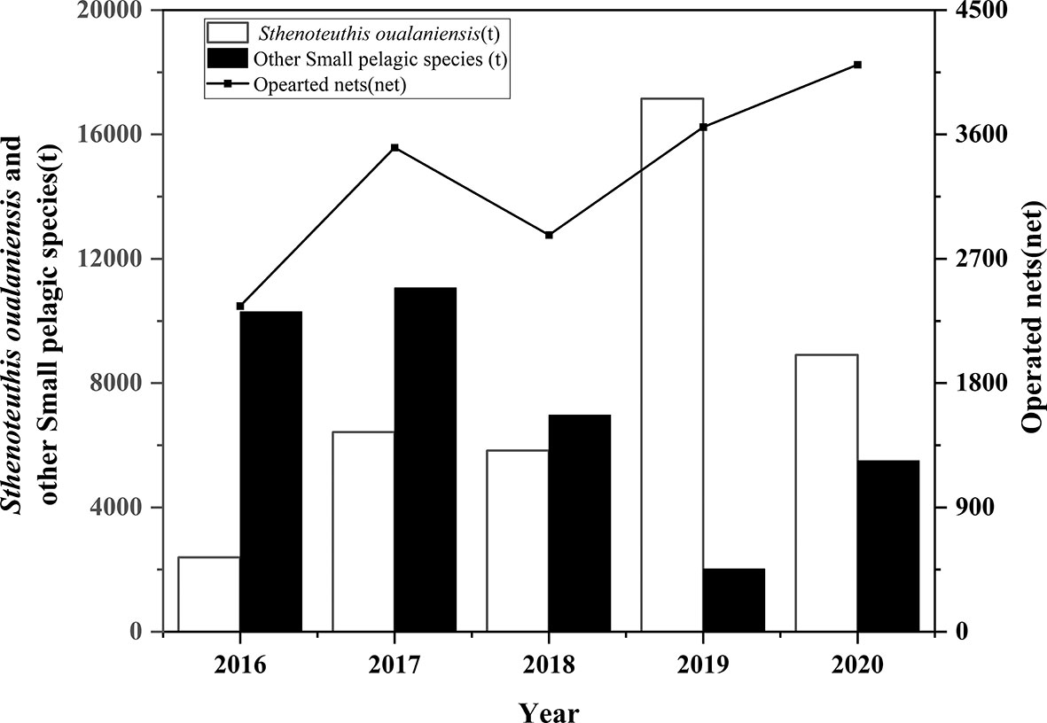
Figure 1 Changes in the main catches and operated nets for light falling gear in the northwest Indian Ocean from 2016 to 2020.
From the annual time scale, from 2016 to 2020, the average yearly CPUE range was 3.51–5.37 t/net, and the proportion of total catches was 16.5%–25%. There were repeated upward and then downward trends in the proportion of catches. The average annual CPUE showed a downward trend, except in 2019 (Figure 2).
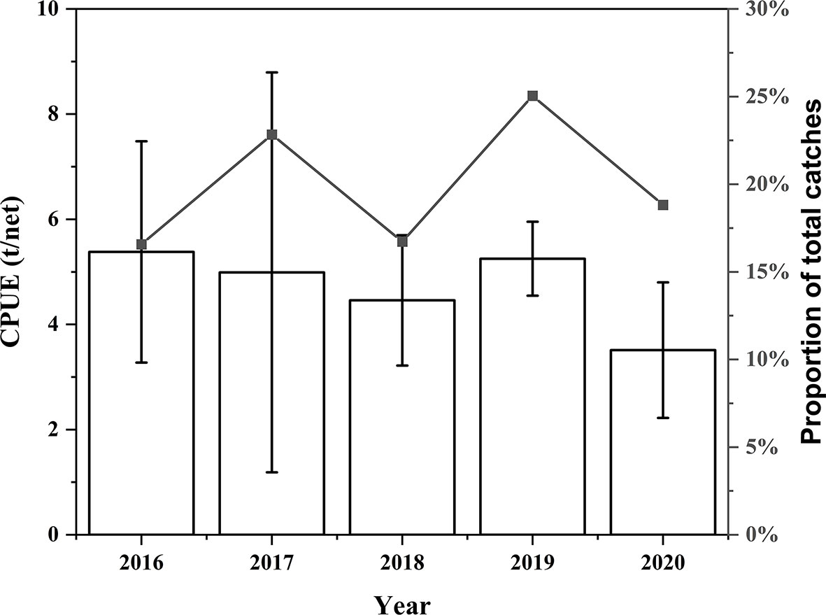
Figure 2 Variation in the proportion of total catches (line) and CPUE (bar) of light falling gear in the Northwest Indian Ocean on a yearly scale (mean ± standard deviation).
From the monthly time scale, the changing trend of the monthly average CPUE and the proportion of total catches were the same from 2016 to 2020. On the whole, the proportion of total catches showed a downward trend in the first part of the year, and in the second half of the year, except for December, it showed an upward trend on the whole; on the whole, the monthly average CPUE showed a downward trend from January to May and an upward trend from September to December. The highest value was November (6.75 t/net), the lowest value was May (2.84 t/net), and the most stable values were from January to March (4.23–4.53 t/net). There was little production from June to August because the southwest monsoon of the Indian Ocean was strong in summer, and the wind and waves were more than 3 m every day. Therefore, the net covering could not be operated, and the fishing was suspended in China (Figure 3).
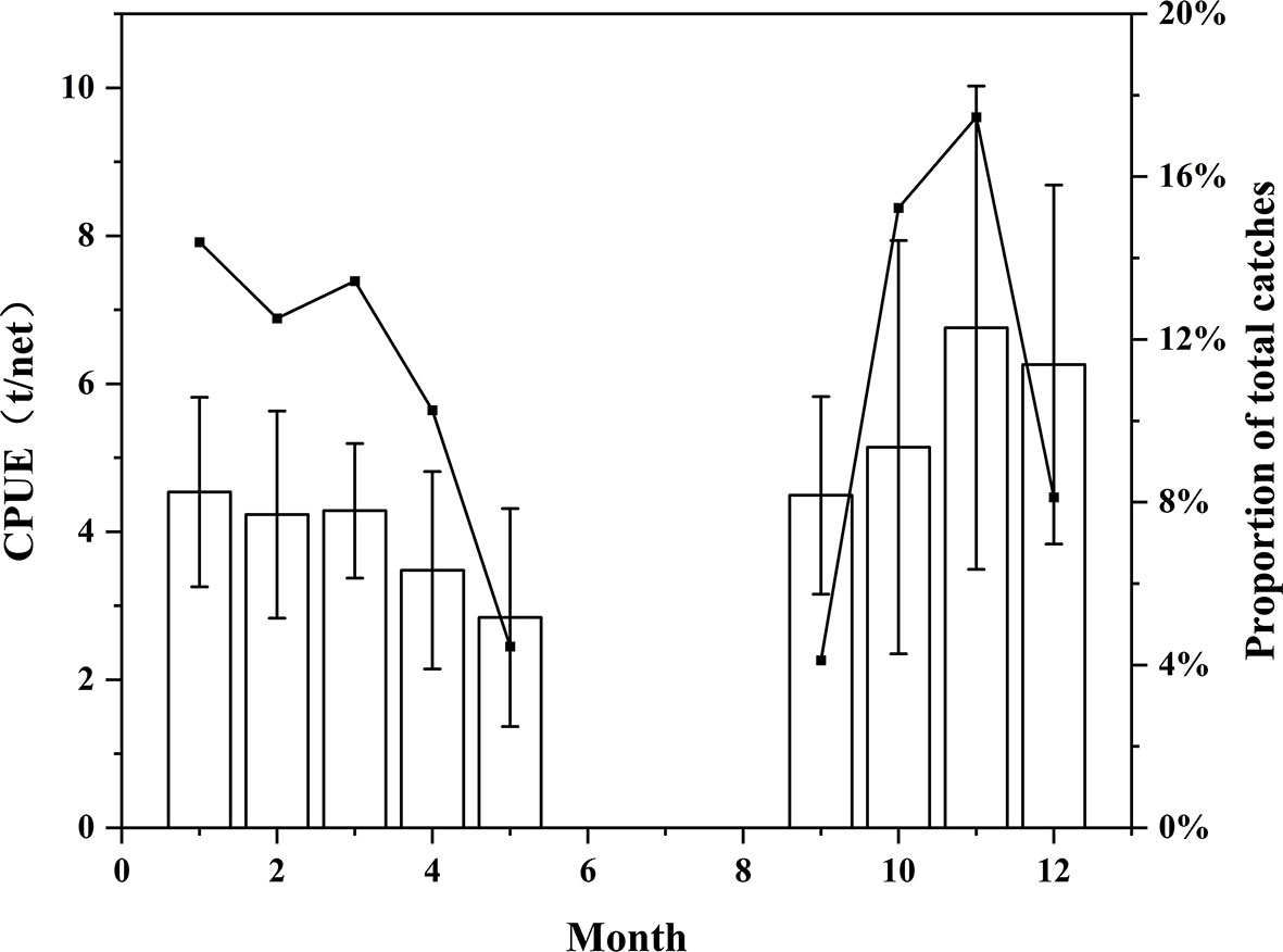
Figure 3 Variation in the proportion of total catches (line) and CPUE (bar) of light falling gear in the Northwest Indian Ocean on a monthly scale (mean ± standard deviation).
From the weekly time scale, there were some different trends in the weekly mean CPUE and the proportion of total catches from 2016 to 2020, with no catch from week 23 to week 36 when the fishery was closed for adjustment back home. The proportion of total catches consistently showed a trend of increasing and then decreasing, with the last 17 weeks (weeks 37 to 53) fluctuating significantly more than the first 18 weeks (weeks 1 to 18). The proportion of total catches varied greatly between weeks, with the highest value of the proportion of total catches being week 47 (4.79%) and the lowest value being week 37 (0.03%). The trend of the mean weekly CPUE was the opposite to the proportion of total catches, repeatedly showing a decreasing trend followed by an increasing trend, where the CPUE values were significantly higher in weeks 37–53 than in weeks 1–22, with the highest value in week 48 (7.42 t/net) and the lowest value in week 22 (1.44 t/net) (Figure 4).
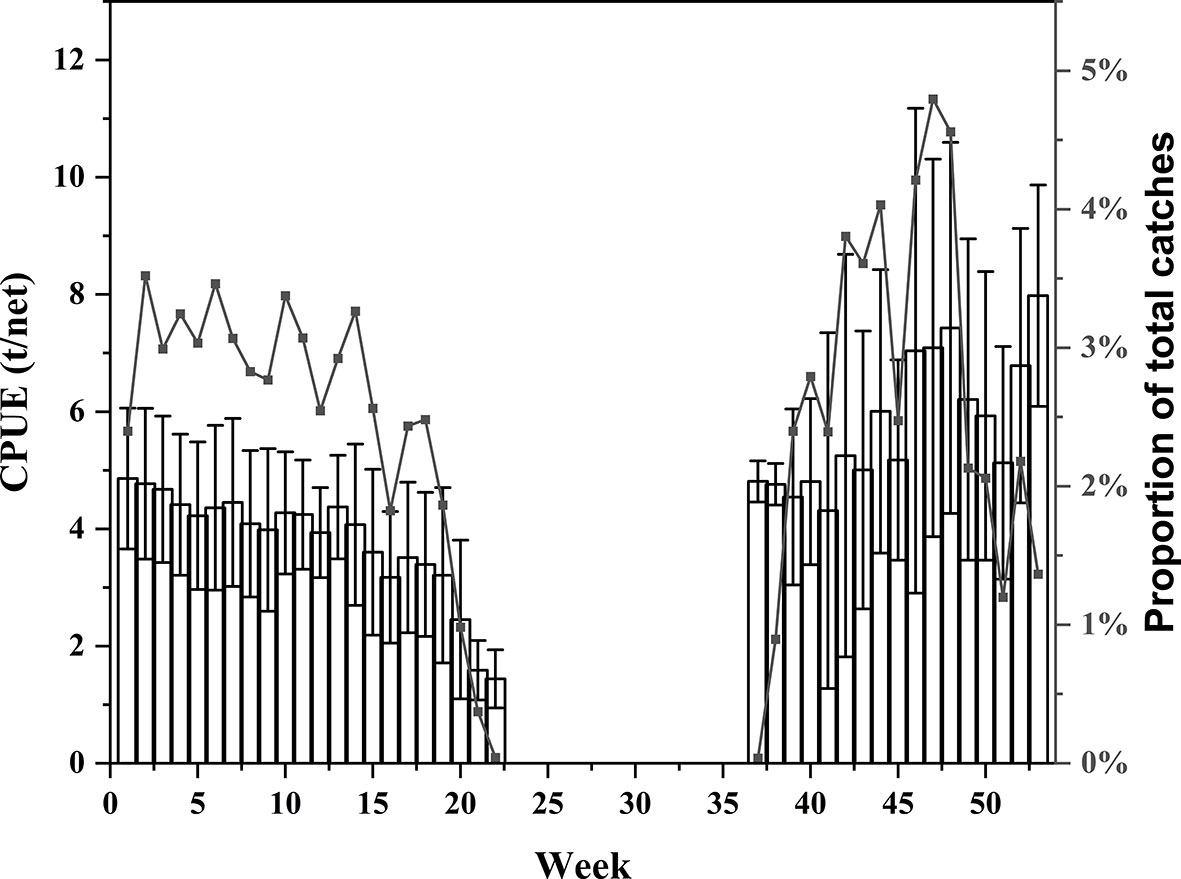
Figure 4 Variation in the proportion of total catches (line) and CPUE (bar) of light falling gear in the Northwestern Indian Ocean on a weekly scale (mean ± standard deviation).
From the perspective of lunar phases, from 2016 to 2020, the proportion of total catches and average CPUE on no moonlight days were significantly higher than on bright moonlight days. The catches on the no moonlight days (49,444.9 t) were about 1.82 times higher than those on the bright moonlight days (27,131.1 t). Among these, the proportion of total catches was higher than 2.6% on no moonlight days. The highest value was on the lunar 24th (4.68%). The proportion of total catches on moonlight days was lower from lunar 12th to lunar 18th, less than 1.1%, and the lowest value was lunar 14th (0.04%). The CPUE of the no moonlight days and bright moonlight days were higher than 4t/net except the 13th to the 15th of the lunar calendar. The highest value was the third day of the no moonlight day (4.8 t/net), and the lowest value was the 14th day of the bright moonlight day (2.06 t/net) (Figure 5).

Figure 5 Variation in the proportion of total catches (line) and CPUE (bar) of light falling gear in the Northwestern Indian Ocean on the lunar phase scale (mean ± standard deviation).
From an operation time scale perspective, the proportion of the total number of catches was higher from 18:00 to 19:59 and from 22:00 to 23:59. In contrast, the proportion of total catches was lower in the rest of the period, especially from 17:00 to 17:59, and generally showed that the proportion of total catches was much higher in the latter half of the night (18:00 to 23:59) than in the first half of the night (0:00 to 5:00). The average CPUE was relatively stable and not very volatile during the operating time. The highest CPUE value was 21:00–21:59 (5.90 t/net), and the lowest value was 18:00–18:59 (4.55 t/net) (Figure 6).
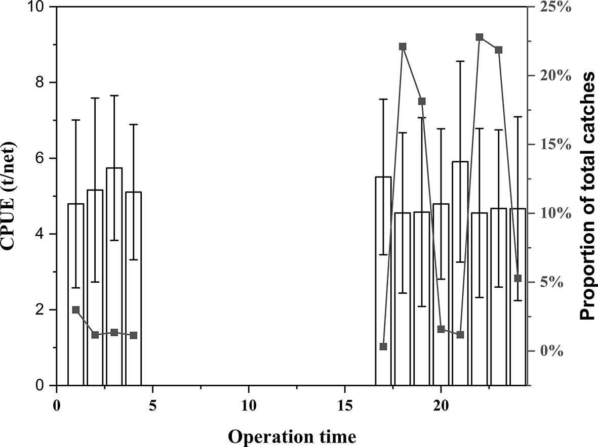
Figure 6 Variation in the proportion of total catches (line) and CPUE (bar) of light falling gear in the Northwestern Indian Ocean under the operation time scale (mean ± standard deviation).
From the perspective of SST (Figure 7A), with sea surface temperature rise, CPUE first increased (24–27 °C) and then decreased (27–32 °C), and the high-value CPUE appeared at 27–28 °C. Most of the catches were concentrated at 25–30 °C. When the sea surface temperature was 31–32 °C, there was almost no catch in the northwest Indian Ocean (Figure 7A). From the perspective of Δ50 (Figure 7B), as the water temperature difference between the two layers increases, CPUE first decreases and then increases. When Δ50 was in the range of −0.2 to −0.15 °C/m, the CPUE value was the highest. Still, the operated nets of this group were the most minor, resulting in the least catches, which had little reference value. Secondly, the second high CPUE value (4.86 t/net) appeared in the range of −0.05 to 0 °C/m, which was also the range with the largest catches (Figure 7B). From the perspective of Chla (Figure 7C), when Chla was in the range of 0 to 0.1 mg/m3, the highest CPUE values were found in the northwest Indian Ocean, indicating a higher density of biological resources in the high range. The catches were the highest in the range of 0.1 to 0.2 m3. The catches were less when Chla ≥0.4 mg/m3 (Figure 7C). From the perspective of SSH (Figure 7D), with the increase of SSH, CPUE first increased (0–0.3 m) and then decreased (0.3–0.6 m). The high CPUE value appeared in the 0.1 to 0.2 m range, and the catches were mainly concentrated in the 0.2–0.4 m range (Figure 7D). From the perspective of SSS (Figure 7E), the high-value CPUE mainly appeared in 35.5–36.5‰, and the operated nets were concentrated primarily in 36–37‰. The high and low salinity were not suitable for the operation of light falling gear in the northwest Indian Ocean (Figure 7E); From the perspective of CV50 (Figure 7F), when the CV50 was less than 0.8, the CPUE would increase with the flow rate. When the CV50 was greater than 0.8, the current would first increase (0.8–1.0 m/s) and then decrease (1.0–1.2 m/s). The high-value CPUE would appear at 0.6–0.8 m/s, and the catch would decrease with the flow rate. The area with large catches and the area with more operated nets would be 0–0.4 m/s (Figure 7F); From the perspective of DO (Figure 7G), CPUE has little difference in each range, and its catches and operated nets were mainly concentrated in 100–160 mmol/m³.Low and high oxygen areas were not high, light falling gear vessels operated few nets, and the catches were less (Figure 7G).

Figure 7 Relationship between CPUE, catches, and environment variables ((A) SST, (B) △50, (C) Chla, (D) SSH, (E) SSS, (F) CV50, (G) DO. mean ± standard deviation).
From the annual time scale, the center of gravity of the fishing grounds changed significantly between 2016 and 2020, with an overall trend towards the northeast, forming two more concentrated areas of the center of gravity of the fishing grounds among 14.7°–16°N, 60.3°–61°E and 16.5°–17.5°N, 62.9°–63.2°E, respectively (Figure 8, 2016–2020).
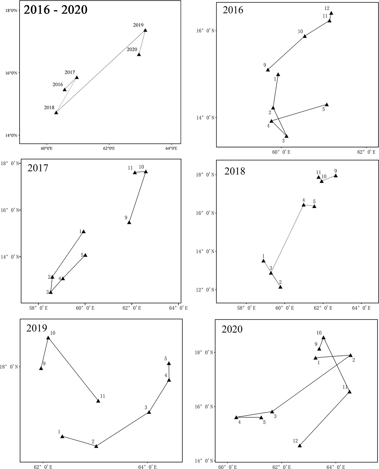
Figure 8 Variation of the center of gravity of the Northwest Indian Ocean light falling gear fishing grounds on a yearly and monthly time scale.
From the time scale of the month, in 2016 (Figure 8, 2016), the center of gravity of the fishery shifted southward from February to March, northwestward in April, and northeastward in May, and from October to December, with a smaller range of changes in the center of gravity in December. In 2017 (Figure 8, 2017), the center of gravity of the fishery shifted to the southwest from February to March and November, and the northeast from April to May and September to October, with a smaller range of change in the center of gravity from March to April and November. In 2018 (Figure 8, 2018), the center of gravity of the fishery shifted southeastward in February and May, northwestward in March, northeastward in April, and westward from October to November. Overall, the change in the center of gravity of the fishery in the second half of the year (September–November) was less than that in the first half of the year (January–May). In 2019 (Figure 8, 2019), the center of gravity of the fishery shifts to the southeast in February and November, and to the northeast from March to May and in October. Compared to 2016 to 2018, the center of gravity of the fishery is at high latitudes throughout 2019. In 2020 (Figure 8, 2020), the center of gravity of the fishing grounds tends to move southwestward from February to May in general, with some months moving eastward. The center of gravity of the fishing grounds moves northeastward in October and southward from November to December. For the first time in 2020, the center of gravity of the fishery shifts significantly southward from October to December relative to the previous four years.
One thousand repeated cross-validation showed that the fitting accuracy of the RF model (R² = 0.709, RMSE = 0.2034) was good, and the prediction accuracy of the model was 55.8% (Figure 9A). The fitting accuracy of the GAM model (R² = 0.632, RMSE = 0.2242), and the prediction accuracy of the model was 37.3%. Overall, the fitting accuracy of the RF model in this study is better than that of the GAM model (Figure 9B).
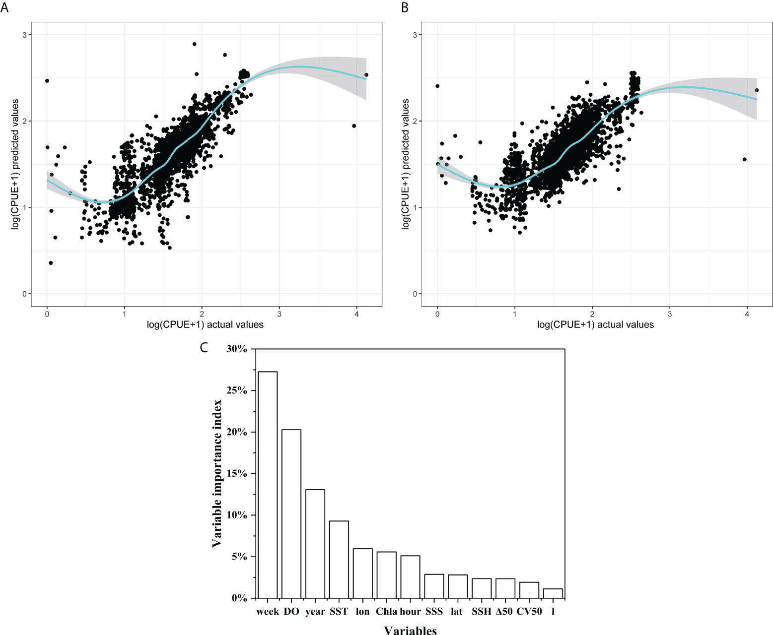
Figure 9 Scatter fitting diagram of RF and GAM models and importance evaluation on variables in RF models. (A) RF model fit diagram, blue fluorescence curve is the fitting curve, the gray area is the confidence interval; (B) GAM model fit diagram, blue fluorescence curve is the fit curve, the gray area is the 95% confidence interval; (C) Importance ranking of variables for RF model.
The RF model explains the impact of time variables in CPUE through the importance evaluation index of independent variables. The significance of the effects of time variables on CPUE in the model is week (27.25%), year (13.06%), operation time (5.11%), and lunar phase (1.12%), (Figure 9C). In the GAM model, the importance of the influence of time variables on CPUE is explained according to the variance interpretation rate. The extent of the impact of time variables on CPUE in the model is week (28.1%), year (13.6%), lunar phase (0.5%), and operation time (0.2%) (Table 1). The results of the two models showed that the time scale of year and week significantly impacted CPUE, and the effects of operation time and lunar phase were smaller. Overall, the importance of the long time scale (year and week) was higher than that of the short time scale (lunar phase and operation time).
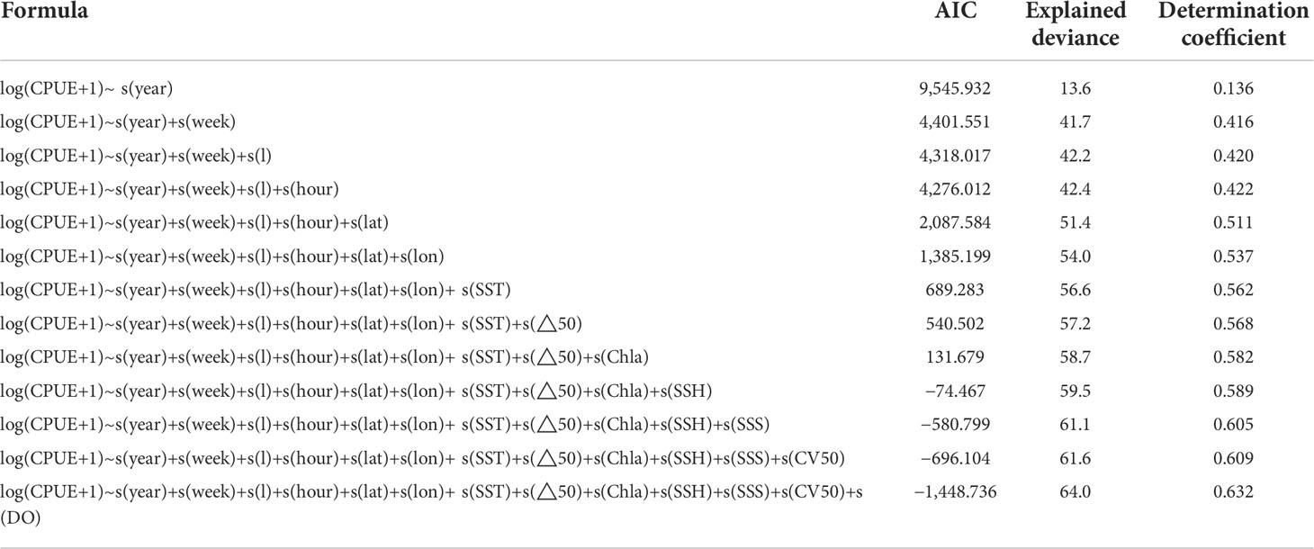
Table 1 GAM model statistical results (Akaike’s Information Criterion, AIC).
The partial dependence diagram of the RF model showed that the fitting curve of the impact of years on the northwest Indian Ocean light falling gear CPUE presented the first trough and then a peak (Figure 10A). With the increase in years, the 95% confidence interval decreased gradually (Figure 10A). The fitting curve of the influence of weeks on CPUE showed a nonlinear positive relationship. Overall, the confidence interval for weeks 37 to 53 was narrower than that for weeks 1 to 22, with marginally higher reliability (Figure 10B). The fitting curve of the influence of the lunar phase relative to CPUE showed an approximate linear negative relationship. The maximum value of CPUE appeared on the no moonlight day, the sixth day of the lunar calendar, and the overall change range was small before and after the 95% confidence interval (Figure 10C). The fitting curve of the impact of operation time on CPUE presented a “U” shape. At 22–24, the 95% confidence interval was small, and the reliability was higher than in other time periods (Figure 10D).

Figure 10 Partial correlation diagram of RF model of the influence of time variables on CPUE. (A) year, (B) week, (C) l, (D) hour, the black curve is the influence curve of variable on CPUE, the blue curve is the fitting of the trend of the influence curve, and the gray area is the 95% confidence interval.
The analysis results of the GAM model showed that: the impact of years on the CPUE of northwest Indian Ocean light falling gear showed a very significant nonlinear negative relationship, in which the confidence interval in 2020 was small and the reliability was slightly higher (P<0.001, Figure 11A); the influence of weeks on CPUE showed a nonlinear relationship. The larger confidence intervals for weeks occurred around 22 and 37 weeks, and the closer to the non-fishing weeks, the lower the reliability (P<0.001, Figure 11B). The influence of the lunar phase on CPUE showed a non-linear relationship. The result of a light moonlight night on CPUE was significantly lower than that of a no-moonlight night. The influence and reliability of lunar calendar 13–15 was the lowest (P<0.001, Figure 11C); the impact of operation time on CPUE showed a fluctuating correlation. The higher peaks appeared at 17–24 h, but the confidence interval was more significant than that at 1–4 h, and the reliability was slightly lower (P<0.001, Figure 11D).

Figure 11 Analysis of the GAM model results of the influence of time variables on CPUE. (A) year, (B) week, (C) l, (D) hour, the solid line is the influence curve and the 95% confidence interval between the two dashed lines.
In this study, longitude (5.96%) in the RF model was slightly more important than latitude (2.80%). In contrast, for the GAM model, latitude (9%) was more critical than longitude (2.6%) (see Figure 9C and Table 1). The partial dependence diagram of the RF model showed that the fitting curve of the influence of latitude on CPUE presented a “trough” type. As the latitude increased, the CPUE of the northwest Indian Ocean light falling gear first decreased and then increased, and its segmentation point appeared at about 15.25°N. The confidence interval between 15.75°N and 16.25°N was less than other latitudes, with high reliability (Figure 12A). The fitting curve of the influence of longitude in CPUE presented a “crest” type, which gradually increased with the increase in longitude. The peak appears at about 65.25°E. Except for the area of 61.25°E–61.75°E, the longitude confidence interval was slightly larger, and the reliability was slightly lower (Figure 12B).
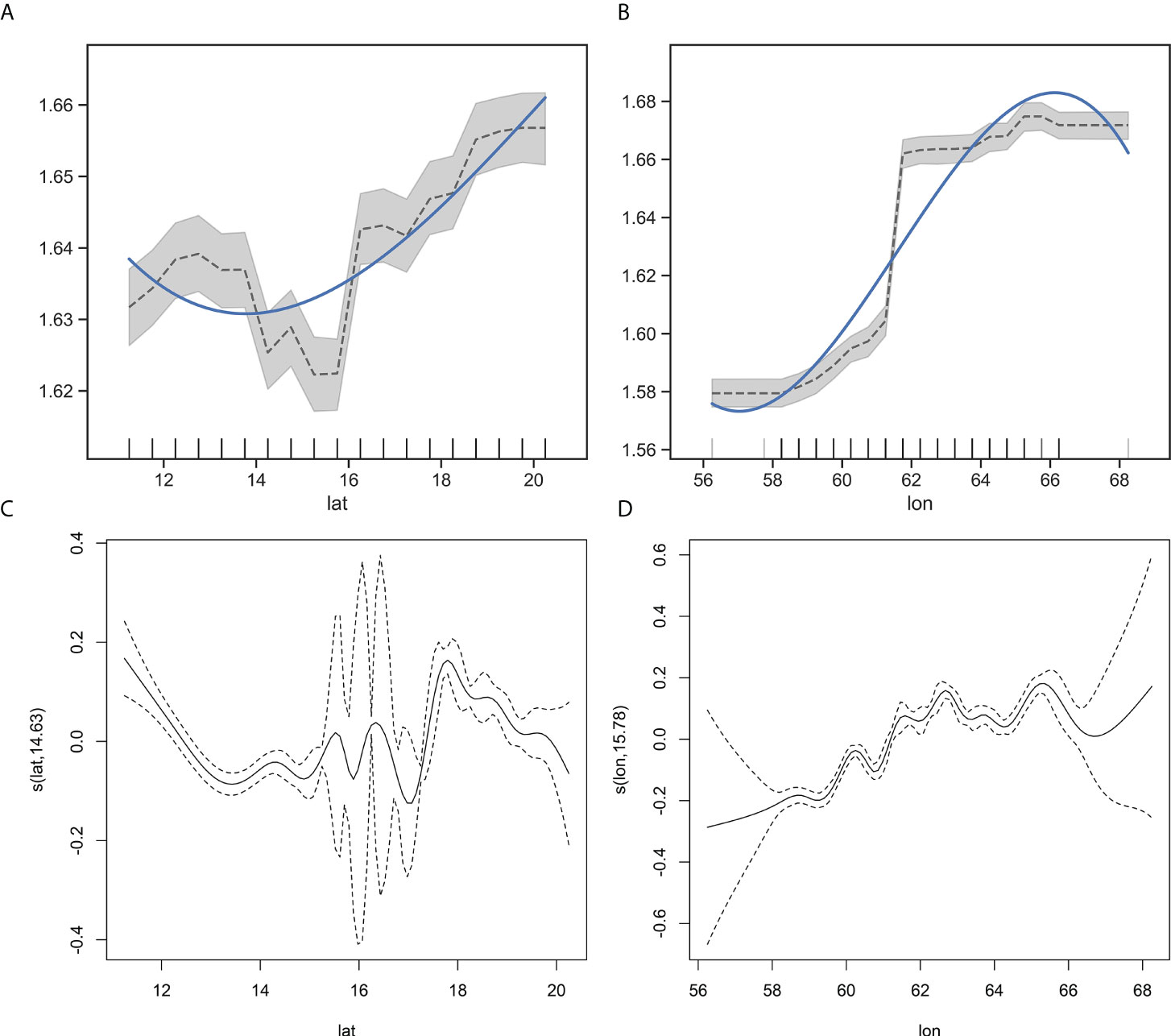
Figure 12 Partial correlation diagram of RF and GAM model of the influence of spatial variables on CPUE. (A) lat, (B) lon, the black curve is the influence curve of variable on CPUE, the blue curve is the fitting of the trend of the influence curve, and the gray area is the 95% confidence interval; (C) lat, (D) lon, the solid line is the influence curve and the 95% confidence interval between the two dashed lines.
The results of the GAM model analysis showed that there was a nonlinear relationship between latitude and CPUE. With the increase in latitude, the impact on the degree of latitude for CPUE repeatedly showed a trend of decreasing first and then increasing. The 95% confidence interval between 17.25°N and 17.75°N was significantly smaller, and the reliability was higher than that of other latitudes (P<0.001, Figure 12C). The longitude and CPUE showed a fluctuating and rising correlation, which gradually increased with the increase in longitude. The 95% confidence interval between 59.25°E and 61.25°E was small, and the reliability was high (P<0.001, Figure 12D).
In this study, the importance of environmental variables on CPUE in the RF model was in the order of DO (20.29%), SST (9.28%), Chla (5.57%), SSS (2.87%), SSH (2.36%), Δ50 (2.35%), and CV50 (1.92%); the importance of environmental variables on CPUE in the GAM model was in the order of SST (2.6%), DO (2.4%), SSS (1.6%), Chla (1.5%), SSH (0.8%), △50 (0.6%), and CV50 (0.5%) (see Figure 9C and Table 1).
The partial dependence diagram of the RF model showed that the fitting curve of SST impact on the northwest Indian Ocean light falling gear CPUE presented a “wave crest” type. With the increase of water temperature, it first increased and then decreased, and the impact on CPUE above 29.6 °C decreased significantly, which was not suitable for light falling gear operation (Figure 13A); The fitting curve of the influence of △50 on CPUE presented the type of “peak before the trough.” On the whole, △50 was inversely proportional to the CPUE of northwest Indian Ocean light falling gear. The CPUE values in the range of −0.10 to −0.06°C/m are the highest, but the confidence interval was large, and the reliability was slightly low (Figure 13B); The fitting curve of Chla’s influence on CPUE showed a gradual downward trend, and the optimal range of Chla was 0.09–0.10 mg/m³, with a small confidence interval and high reliability (Figure 13C). The fitting curve of the SSH impact on CPUE was of the “inverted U” type, which increased first and then decreased. The high value of CPUE appeared at 0.246–0.26 m, the confidence interval was small, the regional interval was small, and the interval was 0.04 m (Figure 13D). The fitting curve of the influence of SSS on CPUE showed a gradual upward trend, and the area with a small confidence interval appeared at 36.03–36.06 and 36.49–36.52, with high reliability (Figure 13E). The fitting curve of the influence of CV50 on CPUE showed a gradual upward trend. The overall confidence intervals were not very different and did not form a continuous region of smaller confidence intervals (Figure 13F); the fitting curve of the impact of DO on CPUE showed the type of “trough first and then peak,” and the confidence interval showed that the optimal DO is 150.6–154.1 mmol/m3(Figure 13G).
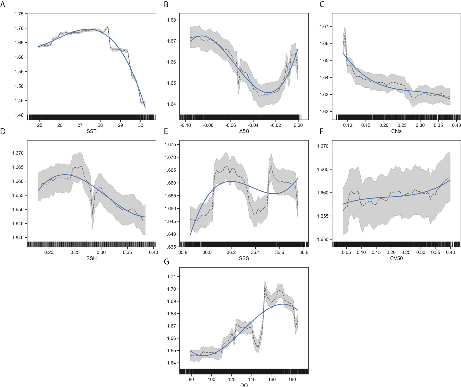
Figure 13 Partial correlation diagram of RF model of the influence of environmental variables on CPUE. (A) SST, (B) △50, (C) Chla, (D) SSH, (E) SSS, (F) CV50, (G) DO, the black curve is the influence curve of variable on CPUE, the blue curve is the fitting of the trend of the influence curve, and the gray area is the 95% confidence interval.
The results of the GAM model analysis showed that SST and northwest Indian Ocean light falling gear CPUE showed a very significant nonlinear relationship, and the confidence interval showed that the more appropriate water temperature was 28.2–28.6 °C and 29.1–29.4 °C. The confidence interval above 29.5 °C increased significantly, and the reliability decreased (P<0.001, Figure 14A). There was a very significant nonlinear relationship between △50 and CPUE. When △50 was −0.10–0 °C/m, the confidence interval tended to be stable, and the reliability was higher than in other ranges (P<0.001, Figure 14B); Chla and CPUE showed a very significant nonlinear positive relationship, and the confidence interval showed that the optimal Chla range was 0.068–0.1 mg/m3 (P<0.001, Figure 14C); SSH and CPUE showed a very significant nonlinear negative relationship, with the lowest confidence interval of 0.24–0.35 m and the highest reliability (P<0.001, Figure 14D); SSS and CPUE showed a non-linear and extremely significant relationship. The confidence interval of salinity 36.1–36.8 was small, and the reliability was high (P<0.001, Figure 14E); CV50 and CPUE showed a very significant nonlinear relationship, and the confidence interval showed that the optimal CV50 range was 0.05–0.2 m/s with high reliability (P<0.001, Figure 14F). There was a very significant nonlinear relationship between DO and CPUE. On the whole, CPUE increased slowly with the increase of DO. Confidence intervals indicate that there are multiple ranges of suitable DO, excluding the low DO and high DO intervals (P<0.001, Figure 14G).
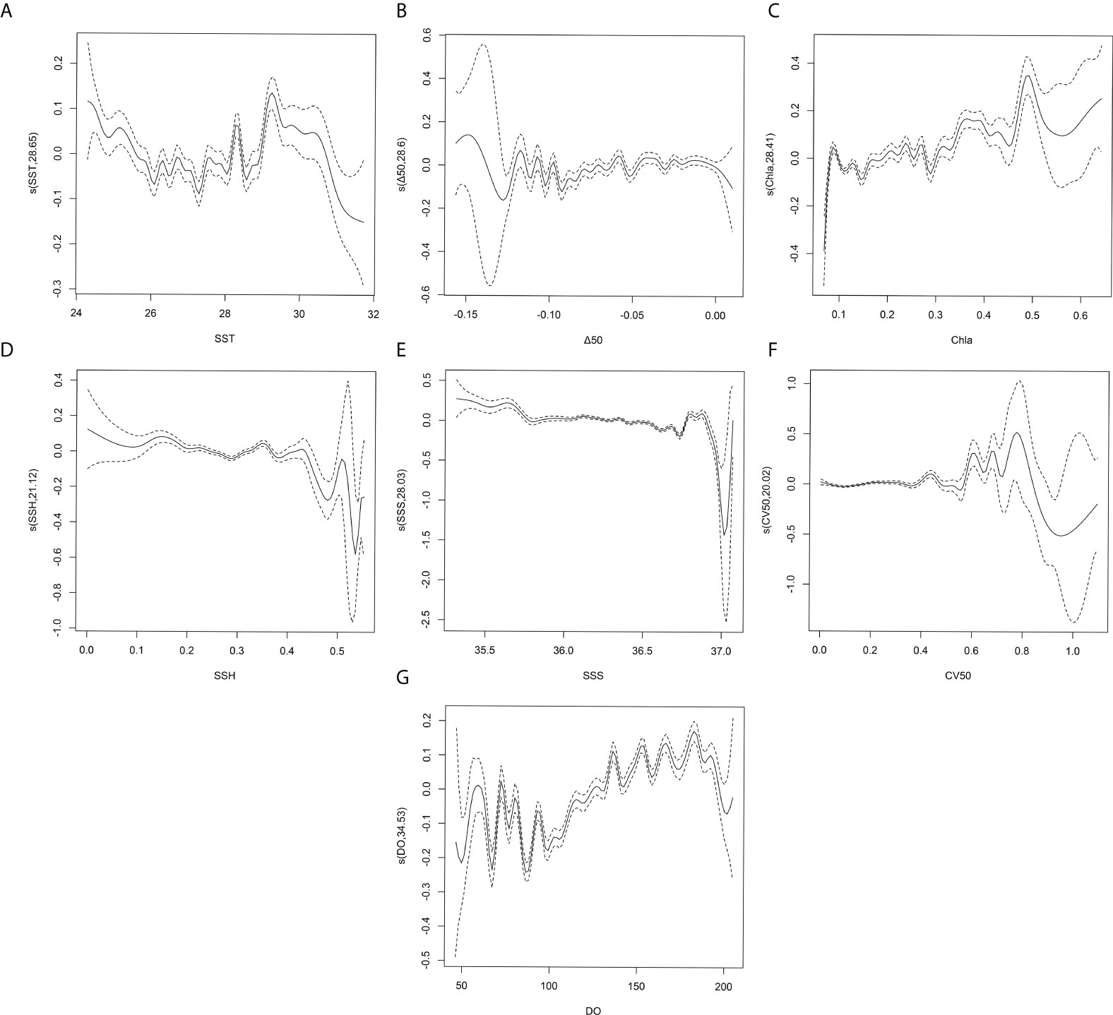
Figure 14 Analysis of the results of the GAM model of the influence of environmental variables on CPUE. (A) SST, (B) △50, (C) Chla, (D) SSH, (E) SSS, (F) CV50, (G) DO, the solid line is the influence curve, and the 95% confidence interval between the two dashed lines.
From 2016 to 2020, the proportion of squid (S. oualaniensis) in the total output increased continuously. It reached its peak in 2019 (89.4%) (Figure 1), which may be related to the discovery of a new squid fishing ground in the northern Indian Ocean by light falling gear vessels in 2019. Relevant studies have also shown that iris squid resources in the north of the Indian Ocean are the most abundant (Pillai et al., 1996; Cui, 2011). At the same time, squids have significant economic and nutritional value. Its low investment risk, strong operability, strong phototropism, and production advantages that can withstand great fishing pressure are also important reasons for it to gradually replace mackerel (S. australasicus) and become the target catch in the Indian Ocean (Roeleveld, 1998; Zhang et al., 2010).
Affected by the monsoon and anti-equatorial current, the Northwest Indian Ocean has formed a wide range of upwelling, making the sea area have high plankton and able to gather more pelagic fish such as squid (S. oualaniensis) and mackerel (S. australasicus). Therefore, the sea area is an important fishing ground for the operation and production of light fishing boats in China (Yang et al., 2019; Wen et al., 2021). The research showed that, on a yearly scale, the output of light falling gear fishing vessels in the northwestern Indian Ocean increased steadily from 2016 to 2019, which is mainly related to the increase in operation frequency, the proportion of catches (Figure 1), and the change of fishing ground gravity center (Figure 8). The decline in output in 2020 was due to the sharp increase in light-falling gear fishing vessels in the sea and increasing fishing pressure; From the monthly and weekly scales, the catches in the second half of the year were significantly higher than those in the first half of the year, which was mainly affected by the large-scale environmental variables of the fishing ground (Yan et al., 2015; Yang et al., 2019a; Wen et al., 2021). The change of CPUE was basically consistent with the regime shift of catch, and the week showed the opposite trend. From the lunar phase scale, the catches on the no moonlight day were significantly higher than those on the bright moonlight day, which was consistent with the research of L. Yan et al. (2015) and Zhao et al. (2019). The lower value of CPUE appeared on the moonlight night from the 11th to 18th of the lunar calendar. From the operation time scale, the higher catches were 18:00–19:59 and 22:00–23:59. The catches in other periods were low, especially 17:00–17:59. This was mainly related to the operation mode of light falling gear (Zhang et al., 2016).
From 2016 to 2020, the output center of the Northwest Indian Ocean changed significantly. Generally, it showed a trend of moving to the northeast, related to the exploration of new fishing grounds by light-falling gear fishing vessels in the Northwest Indian Ocean. The change in squid catch (Figure 1) and relevant studies also showed that the squid resources in the northern Indian Ocean were the most abundant (Pillai et al., 1996; Cui, 2011); the center of gravity of the fishing ground changes first to the south and then to the north, which is related to the seasonal environmental transformation of the Northwest Indian Ocean (Yang et al., 2019; Wen et al., 2021).
Seven marine environmental variables, including SST and SSH, play an essential role in the formation of pelagic fish or squid species on fishing grounds (Yang et al., 2006; Yang et al., 2019a; Li et al., 2020; Xie et al., 2020). Generally, sea surface temperature, sea surface height, and chlorophyll are critical environmental variables affecting the formation of pelagic fish fishing grounds. However, the variables that play a leading role are inconsistent (Yang et al., 2006; Yang et al., 2019b; Li et al., 2020; Xu et al., 2021; Wei et al., 2022).
In this study, the RF model and GAM model showed that the most critical environmental variables affecting the CPUE were DO, SST, SSS, and Chla, and the least important were SSH, Δ50, and CV50. Wei et al. (2022) used the GAM model to study squid (S. oualaniensis) in the Northwest Indian Current and found a significant effect of sea surface temperature on squid. Yang et al. (2019b) used the GAM model to find that the importance of environmental variables on mackerel (S. australasicus) in Arabian Sea lantern light purse seine was SSH, SST, and Chla in turn, while the ocean current had no significant impact on CPUE; Xie et al. (2020) studied the fishing of squid light falling gear off the South China Sea and found that the importance of environmental variables on squid CPUE was SST, SSH, and Chla in turn, but SSS had no significant impact on CPUE; Li et al. (2020) studied the light falling gear fishery in the central and southern South China Sea and found that the importance of environmental variables on CPUE was SST and Δ50 in turn; Staaf et al. (2010) pointed out that the giant squid in the Arabian Sea is related to the hypoxic area. Squid can tolerate the hypoxic environment, but the predators that prey on squid cannot tolerate the hypoxic environment. Therefore, squid has few natural predators and sizeable individual development in the hypoxic area.Therefore, squid has fewer natural enemies and greater ontogeny in low-oxygen areas; Yang et al. (2006) found that the formation of squid fishing grounds in the northwest Indian Ocean is significantly related to SST, Chla, and DO. Based on the above research, SST, Chla, and DO substantially impacted changes in the mackerel and squid fisheries in the Northwest Indian Ocean. With the proportion of squid in the main catches of light falling gear gradually increasing over the year, SST, Chla, and DO can be used as important reference indicators for predicting the light falling gear fishery in the Northwest Indian Ocean. The above conclusions need to be further discussed, and the wind field is not addressed in this study. Relevant studies show that SST, Chla, DO, and monsoon interact (Yang et al., 2006; Staaf et al., 2010; Giddings et al., 2020; Xu et al., 2021). In the later stage, In the later stage, based on more complete light fishing vessel data, we will further explore the influence mechanisms of the marine environment variables in different water layers and variables such as monsoon on the light falling gear fishery and provide scientific methods for the prediction of fishing grounds for light falling gear.
The RF and GAM models were used together to verify each other. They have been widely used in the fields of terrestrial biological resources and ecological environments (Liu et al., 2019a; Stock et al., 2019; Clavel-Henry et al., 2020). However, at present, the accuracy of the evaluation comparison and mutual verification of RF and GAM models is less applied in fishery resources. In this study, RF fitting accuracy is better than that of GAM, which is consistent with the research of Liu et al. (2021) and Kosicki (2020). The above results may be due to the RF model having better performance than the GAM model in controlling the overfitting of the model (Clavel-Henry et al., 2020), as well as the different calculation methods of the two models and the different responses to species density and environmental variables (Kosicki, 2020).
Both RF and GAM results showed that the importance of time variables in the RF model on CPUE was week, year, operation time, and lunar phase; in the GAM model, the importance was followed by a week, year, lunar phase, and operation time. Overall, the importance of the long time scale (year and week) was higher than that of the short time scale (lunar phase and operation time). Xie et al. (2020) used GLM and GAM to study the fishing of squid (S. oualaniensis) in light falling gear off the South China Sea. It was found that the influence of time scale on CPUE was in the order of month and year; Wang et al. (2019) applied the GLM model to study the light falling gear fishing ground in the Beibu Gulf and found that the impact of the annual time scale on CPUE was higher than that of the monthly scale; Li et al. (2020) used the GAM model to study the effect of the discovery scale of squid (S. oualaniensis) in the South China Sea on CPUE, and the importance was lunar phase, operation time and month in turn; Zhao et al. (2019) used GAM model to study iris squid (S. oualaniensis) during spring in the South China Sea. They found that under the same variable conditions, the ratio of lunar phase variance was higher than the operation time, which showed that different sea areas and models would affect the response time scale to CPUE. Therefore, we should use a more comprehensive and accurate time scale for fishery resource assessment and analysis in future resource assessments.
The 95% confidence interval showed that the suitable interval of space (Figure 12) and environmental variables (Figures 13, 14) in the RF model was much smaller than that in the GAM model, which was more accurate and further verifies that the wide range of space and environmental fishery prediction maps was far from meeting the needs of actual production. Therefore, the author suggests that a precise and small range of spatial and environmental variable maps should be used later to predict the fishing ground and guide production operations. For data acquisition reasons, only SST, △50, Chla, SSH, SSS, CV50, and DO were analyzed in this study. Still, the distribution of fisheries is also affected by zooplankton biomass, pH, mixed layer depth, etc. (Wen et al., 2021). Secondly, Guo et al. (2015) further pointed out that integrated models are the best solution to reduce the uncertainty and bias of individual models based on previous experience and that the relationship between temporal, spatial, and environmental variables and high-yield fisheries should be further refined using different integrated models as data completeness and accuracy continue to improve at a later stage. As the number and size of light falling gear vessels tend to increase in the northwest Indian Ocean, it is vital to understand the spatial and temporal distribution patterns of the light falling gear fishery and the environmental variables influencing the variability of the fishery for accurate fishery prediction.
The raw data supporting the conclusions of this article will be made available by the authors, without undue reservation.
HH, CY, and HZ contributed to generating research ideas and writing the essay. ZF contributed to guiding writing and ideas. BJ and BS contributed to model building and data processing analysis. JS and YY for grammar corrections and writing instructions. DX contributed to grammar revision. All authors listed have made a substantial, direct, and intellectual contribution to the work and approved it for publication.
This article is supported by the National Key Research and Development Project of China (2019YFD0901404, 2019YFD0901405), the Central Public-interest Scientific Institution Basal Research Fund, ECSFRCAFS (2021M06), the Zhejiang Ocean Fishery Resources Exploration and Capture Project (CTZB-2021070657), The Yangtze Delta Estuarine Wetland Ecosystem Observation and Research Station, Ministry of Education and Shanghai Science and Technology Committee (ECNU-YDEWS-2020), etc. The study would not have been done without the help of many people. Special thanks go to the ship owners and skippers, who provided details on their fishing gears and technologies used in the analysis.
The authors declare that the research was conducted in the absence of any commercial or financial relationships that could be construed as a potential conflict of interest.
All claims expressed in this article are solely those of the authors and do not necessarily represent those of their affiliated organizations, or those of the publisher, the editors and the reviewers. Any product that may be evaluated in this article, or claim that may be made by its manufacturer, is not guaranteed or endorsed by the publisher.
The Supplementary Material for this article can be found online at: https://www.frontiersin.org/articles/10.3389/fmars.2022.939334/full#supplementary-material
Bucas M., Bergstrom U., Downie A. L., Sundblad G., Gullstrom M., von Numers M., et al. (2013). Empirical modelling of benthic species distribution, abundance, and diversity in the Baltic Sea: evaluating the scope for predictive mapping using different modelling approaches. Ices. J. Mar. Sci. 70 (6), 1233–1243. doi: 10.1093/icesjms/fst036
Chen X., Fan W., Cui X., Zhou W., Tang F. (2013). Fishing ground forecasting of thunnus alalung in Indian ocean based on random forest. Acta Oceanologica. Sin. 35 (01), 158–164. doi: 10.3969/j.issn.0253-4193.2013.01.018
Clavel-Henry M., Piroddi C., Quattrocchi F., Macias D., Christensen V. (2020). Spatial distribution and abundance of mesopelagic fish biomass in the Mediterranean Sea. Front. Mar. Sci. 7. doi: 10.3389/fmars.2020.573986
Cui L. (2011). Shijiedayangxingyuyegaikuang (China ocean press). Available at: http://www.oceanpress.com.cn/.
FAO (2022). “Technical fact sheet for the type of fishing gear,” (FAO Fisheries and Aquaculture). Available at: https://www.fao.org/fishery/en/geartype/217/en.
Giddings J., Matthews A. J., Klingaman N. P., Heywood K. J., Joshi M., Webber B. G. M. (2020). The effect of seasonally and spatially varying chlorophyll on bay of Bengal surface ocean properties and the south Asian monsoon. Weather. Climate Dynamics. 1 (2), 635–655. doi: 10.5194/wcd-1-635-2020
Guo C., Lek S., Ye S., Li W., Liu J., Li Z. (2015). Uncertainty in ensemble modelling of large-scale species distribution: Effects from species characteristics and model techniques. Ecol. Model. 306, 67–75. doi: 10.1016/j.ecolmodel.2014.08.002
Kosicki J. Z. (2020). Generalised dadditive models and random forest approach as effective methods for predictive species density and functional species richness. Environ. Ecol. Stat 27 (2), 273–292. doi: 10.1007/s10651-020-00445-5
Lehodey P., Bertignac M., Hampton J., Lewis A., Picaut J. (1997). El Nino southern oscillation and tuna in the western pacific. Nature 389 (6652), 715–718. doi: 10.1038/39575
Liu X., Feng J., Wang Y. (2019a). Chlorophyll a predictability and relative importance of factors governing lake phytoplankton at different timescales. Sci. Total. Environ. 648, 472–480. doi: 10.1016/j.scitotenv.2018.08.146
Liu J., Jia M., Feng W., Liu C., Huang L. (2021). Spatial-temporal distribution of Antarctic krill (Euphausia superba) resource and its association with environment factors revealed with RF and GAM models. Periodical. Ocean. Univ. China 51 (08), 20–29. doi: 10.16441/j.cnki.hdxb.20200243
Liu Z., Yu J., Chen P., Yu J., Wang Y. (2019). Relationship between the spatio-temporal distribution of light falling-net fishing ground and marine environment in the western guangdong waters. J. South. Agric. 50 (04), 867–874. doi: 10.3969/j.issn.2095-1191.2019.04.26
Li J., Zhang P., Yan L., Wang T., Yang B. (2020). Factors that influence the catch per unit effort of sthenoteuthis oualaniensis in the central-southern south China Sea based on a generalized additive model. J. Fishery. Sci. China 27 (08), 906–915. doi: 10.3724/SP.J.1118.2020.20009
Pillai V. K., Abidi S. A. H., Ravindranathan V., Balachandran K. K., Agadi V. V. (1996). Proceedings of the second workshop on scientific results of FORV sagar sampada. Available at: http://eprints.cmfri.org.in/id/eprint/5233.
Roeleveld M. A. C. (1998). The status and importance of cephalopod systematics in southern Africa. Afr. J. Mar. Sci. 20(1):1–16. doi: 10.2989/025776198784126296
Staaf D. J., Ruiz-Cooley R. I., Elliger C., Lebaric Z., Campos B., Markaida U., et al. (2010). Ommastrephid squids (Sthenoteuthis oualaniensis and dosidicus gigas) in the eastern pacific show convergent biogeographic breaks but contrasting population structures. Mar. Ecol. Prog. 418 (NOV.18), 165–178. doi: 10.3354/meps08829
Stock B. C., Ward E. J., Thorson J. T., Jannot J. E., Semmens B. X. (2019). The utility of spatial model-based estimators of unobserved bycatch. Ices. J. Mar. Sci. 76 (1), 255–267. doi: 10.1093/icesjms/fsy153
Su L., Chen Z., Zhang P., Li J., Wang H., Huang J. (2018). Catch composition and spatial-temporal distribution of catch rate of light falling-net fishing in central and southern south china sea fishing ground in 2017. South China Fisheries. Sci. 14 (05), 11–20. doi: 10.3969/j.issn.2095-0780.2018.05.002
Su L., Chen Z., Zhang k., Zhang J., Wang X. (2018a). Catch composition and spatial-temporal distribution of catch rate of light falling-net fishing in the abysmal area of the northern south China Sea. Mar. Fisheries. 40 (05), 537–547. doi: 10.13233/j.cnki.mar.fish.2018.05.004
Tian S., Chen X. (2010). Impacts of different calculating methods for nominal CPUE on CPUE standardization. J. Of. Shanghai. Ocean. Univ. 19 (02), 240–245.
Wang Y., Yu J., Chen P., Yu J., Liu Z. (2019). Relationship between spatial-temporal distribution of light falling-net fishing ground and marine environments. J. Trop. Oceanography. 38 (05), 68–76. doi: 10.11978/2018129
Wei Q., Cui G., Xuan W., Tao Y., Su S., Zhu W. (2022). Effects of sst and chl-a on the spatiotemporal distribution of sthenoteuthis oualaniensis fishing ground in the northwest indian ocean. J. Fishery. Sci. China 29 (03), 388–397. doi: 10.12264/JFSC2021-0521
Wen L., Zhang H., Fang Z., Chen X. (2021). Spatial and temporal distribution of fishing ground of sthenoteuthis oualaniensis in northern Indian ocean with different fishing methods. J. Of. Shanghai. Ocean. Univ. 30 (06), 1079–1089. doi: 10.12024/jsou.20210103264
Xie E., Zhou Y., Feng F., Wu Q. (2020). Catch per unit effort (CPUE) standardization of purpleback flying squid sthenoteuthis oualaniensis for Chinese large-scale lighting net fishery in the open sea of south China Sea. J. Dalian. Fisheries. Univ. 35 (03), 439–446. doi: 10.3969/10.16535/j.cnki.dlhyxb.2019-122
Xu S., Tang F., Ren H., Li Z., He L. (2021). Phylogenetic relationship and population genetic structure of sthenoteuthis oualaniensis in the Eastern Indian ocean based on cytb gene. J. Of. Shanghai. Ocean. Univ. 30 (06), 970–980. doi: 10.12024/jsou.20210303316
Yadav V. K., Jahageerdar S., Adinarayana J. (2020). Use of different modeling approach for sensitivity analysis in predicting the catch per unit effort (CPUE) of fish. Indian J. Geo-Marine. Sci. 49 (11), 1729–1741.
Yang X., Chen X., Zhou Y., Tian S. (2006). A marine remote sensing-based preliminary analysis on the fishing ground of purple flying squid sthenoteuthis oualaniensis in the northwest Indian ocean. J. Fisheries. China 05, 669–675. doi: 10.3321/j.issn:1000-0615.2006.05.014
Yang S., Fan X., Tang F., Cheng T., Fan W. (2019a). Relationship between spatial-temporal distribution of scomber australasicus and environmental factors in the Arabian Sea. J. Trop. Oceanography. 38 (04), 91–100. doi: 10.11978/2018106
Yang S., Fan X., Wu Y., Zhou W., Wang F., Wu Z., et al. (2019b). The relationship between the fishing ground of mackerel (Scomber australasicus) in Arabian Sea and the environment based on GAM model. Chin. J. Ecol. 38 (08), 2466–2470. doi: 10.13292/j.1000-4890.201908.032
Yang S., Fan X., Zhang B., Zhang H., Zhang S., Cui X., et al. (2019). Spatial-temporal distribution of purse seine in arabian sea and its relationship with sea surface environmental factors. J. Agric. Sci. Technol. 21 (09), 149–158. doi: 10.13304/j.nykjdb.2018.0615
Yan M., Zhang H., Fan W., Jin S., Yang S. (2015). Spatial-temporal CPUE profiles of the albacore tuna (Thunnus alalunga) and their relations to marine environmental factors in the south pacific ocean. Chin. J. Ecol. 34 (11), 3191–3197. doi: 10.1023/10.13292/j.1000-4890.20151023.019
Yan L., Zhang P., Yang L., Yang B., Chen S., Li Y., et al. (2015a). Effect of moon phase on fishing rate by light falling-net fishing vessels of symplectoteuthis oualaniensis in the south China Sea. South China Fisheries. Sci. 11 (03), 16–21. doi: 10.3969/j.issn.2095-0780.2015.03.003
Zhang H., Wu Z., Zhou W., Jin S., Zhang P., Yan L., et al. (2016). Species composition, catch rate and occurrence peak time of thunnidae family in the fishing ground of light falling-net fisheries in the nansha islands area of the south China Sea. Mar. Fisheries. 38 (02), 140–148. doi: 10.13233/j.cnki.mar.fish.2016.02.004
Zhang P., Yang L., Zhang X., Tan Y. (2010). The present status and prospect on exploitotion of tuna and squid fishery resources in south China Sea. South China Fisheries. Sci. 6 (01), 68–74. doi: 10.3969/j.issn.1673-2227.2010.01.012
Zhang P., Zeng X., Yang L., Peng C., Zhang X., Yang S., et al. (2013). Analyses on fishing ground and catch composition of large-scale light falling-net fisheries in south China Sea. South China Fisheries. Sci. 9 (03), 74–79. doi: 10.3969/j.issn.2095-0780.2013.03.012
Keywords: northwest Indian Ocean, catch per unit effort, time scale, environment factors, random forest model, generalized additive model
Citation: Han H, Yang C, Zhang H, Fang Z, Jiang B, Su B, Sui J, Yan Y and Xiang D (2022) Environment variables affect CPUE and spatial distribution of fishing grounds on the light falling gear fishery in the northwest Indian Ocean at different time scales. Front. Mar. Sci. 9:939334. doi: 10.3389/fmars.2022.939334
Received: 09 May 2022; Accepted: 18 July 2022;
Published: 11 August 2022.
Edited by:
Valentina Melli, Technical University of Denmark, Lyngby, DenmarkReviewed by:
Valeria Mamouridis, Independent Researcher, Rome, ItalyCopyright © 2022 Han, Yang, Zhang, Fang, Jiang, Su, Sui, Yan and Xiang. This is an open-access article distributed under the terms of the Creative Commons Attribution License (CC BY). The use, distribution or reproduction in other forums is permitted, provided the original author(s) and the copyright owner(s) are credited and that the original publication in this journal is cited, in accordance with accepted academic practice. No use, distribution or reproduction is permitted which does not comply with these terms.
*Correspondence: Heng Zhang, emhhbmd6aXFpYW4wNjAxQDE2My5jb20=; Zhou Fang, emZhbmdAc2hvdS5lZHUuY24=
†These authors have contributed equally to this work
Disclaimer: All claims expressed in this article are solely those of the authors and do not necessarily represent those of their affiliated organizations, or those of the publisher, the editors and the reviewers. Any product that may be evaluated in this article or claim that may be made by its manufacturer is not guaranteed or endorsed by the publisher.
Research integrity at Frontiers
Learn more about the work of our research integrity team to safeguard the quality of each article we publish.