 Oscar Dario Beltran-Perez
 Joanna J. Waniek
- Department of Marine Chemistry, Leibniz Institute for Baltic Sea Research Warnemünde, Rostock, Germany
Changes in environmental conditions may have an effect on the occurrence and intensity of phytoplankton blooms. However, few studies have been carried out on this subject, mainly due to the lack of long-term in situ observations. We study the inter-annual variability and phenology of spring and summer blooms in the eastern Baltic Sea using a physical-biological model. The one-dimensional NPZD model simulates the development of both blooms in the water column with realistic atmospheric forcing and initial conditions representative of the eastern Baltic Sea between 1990 and 2019. On average, the spring bloom started on day 85 ± 7, reached its maximum biomass on day 115 ± 6 and declined after day 144 ± 5. The summer bloom started on day 158 ± 5, had its maximum biomass on day 194 ± 9 and ended after day 237 ± 8. The results showed that the summer bloom occurs 9 days earlier and last 15 days longer over the 30-year simulation period, but changes in the phenology of the spring bloom were not statistically significant. There is strong evidence that warmer periods favor both blooms, but in different ways. Warmer periods caused spring blooms to peak earlier, while summer blooms reached higher abundance. Additionally, a higher energy gain by the ocean led to longer summer blooms of greater abundance and higher biomass maxima. Overall, summer blooms are more sensitive to changes in the environment than spring blooms, being therefore more vulnerable to changes generated by climate change in the Baltic Sea.
Introduction
The phytoplankton growing season plays an integral role in the marine food web and ecosystem functioning, as phytoplankton comprises the base of the marine food web and represents 90% of ocean productivity (Smith and Hollibaugh, 1993). Phenology studies describe the key stages of the life cycle of species, e.g. seed sprouting, bird migration or phytoplankton growth. Many phenological events are seasonal and therefore they provide insight about the sensitivity of an ecosystem to environmental change. Alteration in phytoplankton phenology may influence the survival of higher trophic levels due to variations in the timing of food availability (match-mismatch hypothesis) (Smith and Hollibaugh, 1993; Winder and Schindler, 2004). Regular phytoplankton blooms occur in all sub-basins of the Baltic Sea, frequently during spring and summer seasons. However, there is still uncertainty about the phenology and factors governing the development of those blooms.
Overall, diatoms dominate the spring bloom but in the Baltic Sea diatoms and dinoflagellates occur at the same time and build up the spring bloom biomass (Klais et al., 2011). The last decades have shown a highly variable proportion of diatoms and dinoflagellates in the spring bloom of the Baltic Sea in both time and space (Klais et al., 2011). Therefore, no common pattern can be defined for all sub-basins, indicating a strong influence of local mechanisms driving the bloom. The conditions, factors and mechanisms promoting the success of cold-water dinoflagellates in dominating the spring phytoplankton community remain poorly understood, as well as their conspicuous dominance in the ice-free central part of the Baltic Sea (Klais et al., 2011). Diatom and dinoflagellate blooms are difficult to track independently with low frequency data due to the co-occurrence of both species, diatom blooms growth faster, but dinoflagellate blooms may last longer (Lips et al., 2014).
The decrease in availability of dissolved silica (DSi) and the reduction of DSi:N ratios associated with eutrophication (Rahm et al., 1996; Papush and Danielsson, 2006) have been suggested to limit diatom growth in the Baltic Sea, indirectly supporting the expansion of dinoflagellate blooms. However, it was shown that spring bloom species in the Baltic Sea are well adapted to low DSi availability and are not directly affected by reduced surface concentrations of DSi (Spilling et al., 2010). Diatoms are effectively seeded even from minor inocula of resting propagules (McQuoid and Godhe, 2004), as in the Gotland Basin where the permanent halocline (at 60–80 m depth) is a strong barrier for local cyst re-suspension from the sediment to the euphotic layer. Additionally, the anoxic sediments and bottom waters are not favorable for cyst germination (Rengefors and Anderson, 1998; Kremp and Anderson, 2000). Small fast-growing diatoms thrive in unstable, turbulent conditions giving them a competitive advantage through building a superior head-start biomass over slow-growing, large and motile dinoflagellates that require a specific habitat setting for bloom formation (Klais et al., 2011).
Spring blooms develop from the south to the north of the Baltic Sea, with the first blooms peaking in mid-March in the Bay of Mecklenburg and the last blooms occurring in mid-April in the Gulf of Finland (Groetsch et al., 2016) and in May/June in the Bothnian Bay with biomass much lower than in most other parts of the Baltic Sea (Spilling et al., 2018). Despite the phenological changes by sub-basin, the bloom length is similar between basins (43 ± 2 day), except for the Bay of Mecklenburg (36 ± 11 day) (Groetsch et al., 2016). Summer blooms are dominated by the cyanobacteria species Nodularia spumigena, Aphanizomenon sp. and Dolichospermum spp. Studies in the Baltic Sea have observed an increase in the intensity and duration of cyanobacteria blooms since the 1960s (Bianchi et al., 2000; Poutanen and Nikkilä, 2001; Kahru and Elmgren, 2014; Kahru et al., 2016; HELCOM/Baltic Earth, 2021). Cyanobacteria blooms give rise to environmental concern due to their ability to fix molecular nitrogen from the atmosphere and the production of toxins by some species that may lead to the death of mammals, fish and filtering organisms in the water (Paerl, 2014). Cyanobacteria blooms usually begin in June and reach their maximum biomass during July and August (Kahru et al., 2020; Beltran-Perez and Waniek, 2021).
Although environmental management programs (e.g. Helsinki Convention, EU Marine Strategy Framework Directive, Baltic Sea Action Plan) have been in place in the Baltic Sea to monitor and control its environmental state for decades, massive blooms continue to occur especially those that produce toxins (Paerl, 2014; Munkes et al., 2020). Eutrophication by nutrients entering the Baltic Sea through rivers, nitrogen fixation from the atmosphere by cyanobacteria species, the organic material subsequently sinking to depth and the turnover of phosphorus from sediments (Vahtera et al., 2007; Paerl and Scott, 2010) are still the major concerns of the environmental authorities in the Baltic Sea (HELCOM/Baltic Earth, 2021). Subsequent remineralization at depth by bacteria depletes oxygen concentration and creates low-oxygen conditions that are lethal to fish (Gustafsson, 2012; Breitburg et al., 2018). Another concern are increasing temperatures, which have been linked to changes in phytoplankton dynamics in terms of abundance, composition and phenology (Carey et al., 2012; HELCOM/Baltic Earth, 2021).
Despite the regular occurrence of spring and summer blooms in the Baltic Sea and their role in the ecosystem, species-specific life cycles, succession and bloom alterations under changing environmental conditions are still not well understood, partly due to the lack of long-term in situ data sets. In recent decades, coupled biological-physical models have been used to define how the phenology of blooms is affected by environmental forcing in different coastal (Sharples et al., 2006; Ji et al., 2008) and marine environments (Hashioka et al., 2009; Henson et al., 2009; Gittings et al., 2018), including the Baltic Sea (Neumann et al., 2012; Dzierzbicka-Głowacka et al., 2013; Daewel and Schrum, 2017). Models include processes on different spatial and temporal scales, their complexity increases depending on the number of processes included and parametrization used. One-dimensional models may provide insight into the mechanisms driving phytoplankton phenology when the dynamics are dominated by local forcing (Sharples et al., 2006) such as in the Baltic Sea, where there are significant changes in the environmental conditions (e.g. in terms of temperature, stratification, mixing) from one basin to another (Schneider and Müller, 2018; Hjerne et al., 2019; HELCOM/Baltic Earth, 2021) regulating the bloom.
Usually phenological studies and models include temperature, solar radiation and wind among other factors as the main bloom drivers, but not heat flux. It has recently been observed that heat flux plays an important role in bloom phenology (Gittings et al., 2018; Beltran-Perez and Waniek, 2021). Our model seeks to define the influence of atmospheric forcing on bloom phenology. Therefore, realistic atmospheric forcing (wind, air temperature, solar radiation, relative humidity, cloud cover) was used in the simulation of the heat budget and energy transfer from the atmosphere to the water column and vice versa. In this study, we hypothesize that (1) the inter-annual variability of spring and summer blooms can be reproduced by a one-dimensional (water column) model including the main forcing affecting bloom formation and biological interactions between phytoplankton, zooplankton, detritus and nutrients, and (2) the phenology of spring and summer blooms has changed, leading to longer and more intense bloom as a consequence of changes in heat flux in the Gotland Basin.
Methods
Study Site
The Baltic Sea is a shallow, semi-enclosed brackish sea in northern Europe (Figure 1). Its drainage basin is shared by 14 countries (around 84 million people), which exerts pressure on all the Baltic Sea ecosystem by increasing eutrophication, pollution and pressure on fish stocks (HELCOM, 2018). The limited water exchange with the North Sea results in a long residence time and a large seasonal and spatial variation in the biological, physical and chemical properties of the water column and the distribution of phytoplankton species (Schneider and Müller, 2018). The high buffer capacity of the system has led to a slow response to nutrient load reductions implemented for decades by the Baltic Sea countries (Savchuk, 2018; Murray et al., 2019). Furthermore, climate change affects the entire ecosystem causing increasing temperatures, declining ice cover and increasing annual precipitation in the Baltic Sea (HELCOM/Baltic Earth, 2021). Therefore, human-induced environmental pressures coupled with climate change may exacerbate changes in the phytoplankton community, especially in the Baltic Sea where the sea surface temperature is increasing faster than the average for the global ocean (HELCOM/Baltic Earth, 2021).
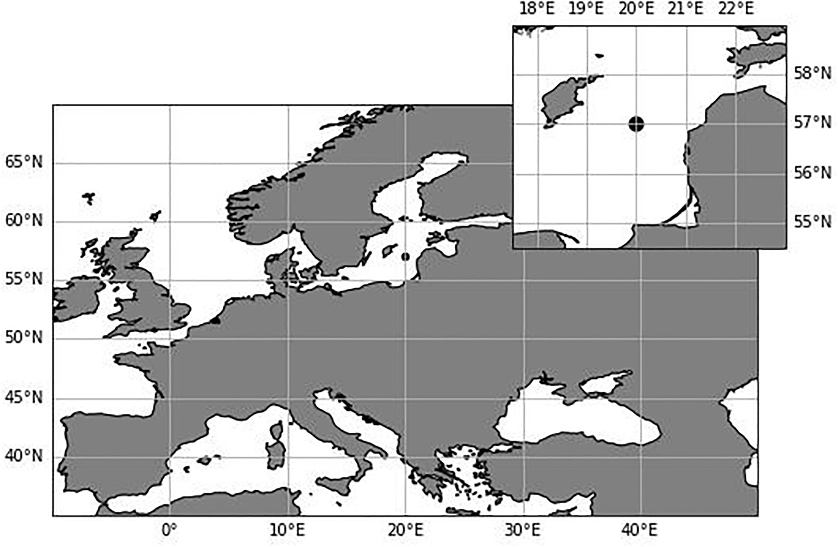
Figure 1 Location of the monitoring station TF271 (black dot) in the Gotland Basin, Baltic Sea.
The Baltic Sea is divided into 17 basins, each basin with its own complexity and particular characteristics (Hjerne et al., 2019; HELCOM/Baltic Earth, 2021). The Gotland Basin is the deepest basin in the Baltic Sea with a maximum depth of 249 m, characterized by a permanent halocline at 60–80 m depth which functions as a barrier between anoxic sediments and bottom waters and the euphotic layer (Klais et al., 2011). Low oxygen levels lead to the production of hydrogen sulphide and release of phosphate from the sediments to the water column which further amplifies primary production and consequently oxygen demand (Vahtera et al., 2007; Murray et al., 2019). This study focuses on the Gotland Basin, specifically the station TF271 (Figure 1) located in the eastern part of the Baltic Sea at 57°19’12” N, 20°3’0” E. This station has been monitored since 1979 in the frame of the HELCOM monitoring program (HELCOM, 2012). However, regular monitoring of blooms began only in 1990 (Wasmund, 1997).
Model-Based Approach
We used a coupled physical-biological model to understand the interactions between the physical and biological conditions of the water column that affect the development of spring and summer blooms in the Gotland Basin. This model is an adaptation of an early version developed by Waniek (2003) to study the physical factors controlling phytoplankton growth in the northeast Atlantic and the Irminger Sea (Waniek, 2003; Waniek and Holliday, 2006). The physical model basically consists of an integrated mixed-layer model for the surface layer embedded into an advective-diffusion model for the thermocline. The model is therefore able to estimate the changes in temperature with depth from kinetic energy and thermal budgets solving wind mixing, convection, upwelling and turbulent diffusion processes in the water column, giving a reliable approach to the physical processes that influence bloom formation. In addition to the changes in the water column, the model incorporates the feedback between the water surface and the atmosphere through the net heat flux terms (incoming solar radiation, long-wave radiation, sensible and latent heat flux) calculated from standard bulk formulae for each time step. A detailed description of the physical model can be found in Waniek (2003).
The biological model is a simplified representation of the phytoplankton cycle conceived primarily to describe the dynamics of six state variables (Figure 2): nitrogen concentration as limiting nutrient, two functional groups of phytoplankton composed of diatoms (Diatoms) and cyanobacteria (Cyano), zooplankton (Zoo) fueled by grazing on mainly diatoms, and detritus, which sinks at two different velocities and is remineralized or lost to the sediment (see Figure 2). In this study the spring bloom was modeled on the basis of diatoms because they usually begin the spring bloom and are considered superior to dinoflagellates as competitors because of their relatively high growth rates and nutrient uptake capacities (Suikkanen et al., 2011). Furthermore, reliable, high frequency data to identify and validate the beginning and end of each bloom individually are still scarce in the Gotland Basin (Klais et al., 2011; Lips et al., 2014). Therefore, the results may combine the behavior of diatoms and dinoflagellates, as both species have basically comparable nutrient requirements (excluding the need for silica) and appear to provide similar ecosystem services with respect to the annual new production and nutrient uptake (Kremp et al., 2008; Klais et al., 2011). All concentrations in the biological model are expressed in terms of nitrogen, i.e. mmol N m–3, as nitrogen is usually the limiting nutrient in the ocean and the common unit in coupled models (Janssen et al., 2004; Beckmann and Hense, 2007; Sonntag and Hense, 2011; Hense et al., 2013). Carbon and phosphate concentrations were transformed into nitrogen using the Redfield ratio between carbon, nitrogen and phosphorus (C:N:P) of 106:16:1 (Redfield, 1958).
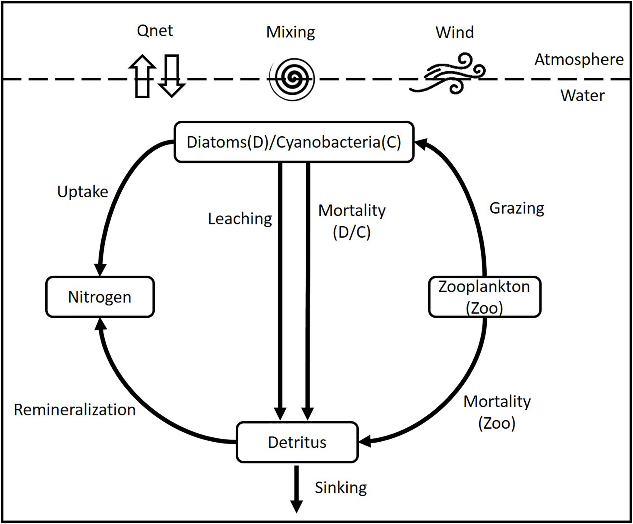
Figure 2 Scheme of the coupled physical-biological model.
The growth rate of phytoplankton is determined by a “Michaelis-Menten” equation, which depends on the availability of nutrients and light (Tables 1, 2). The light term depends on the maximum growth rate of phytoplankton (µgrowth), on the slope of the growth-light curve (α) and the light intensity in the water column. The light in the water column is given by the fraction of photosynthetically active radiation (PAR), the incoming solar radiation (QSW) and the attenuation of light through the water column due to water (kw) and chlorophyll a (kchl). The sink terms for phytoplankton are grazing by zooplankton, leaching and mortality including viral lysis and extracellular release (μm).
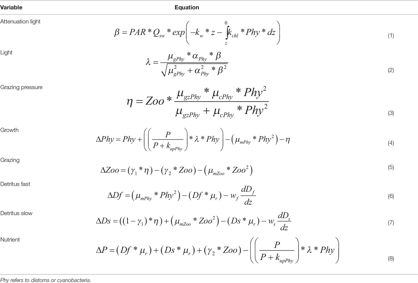
Table 1 Equations of the biological model.
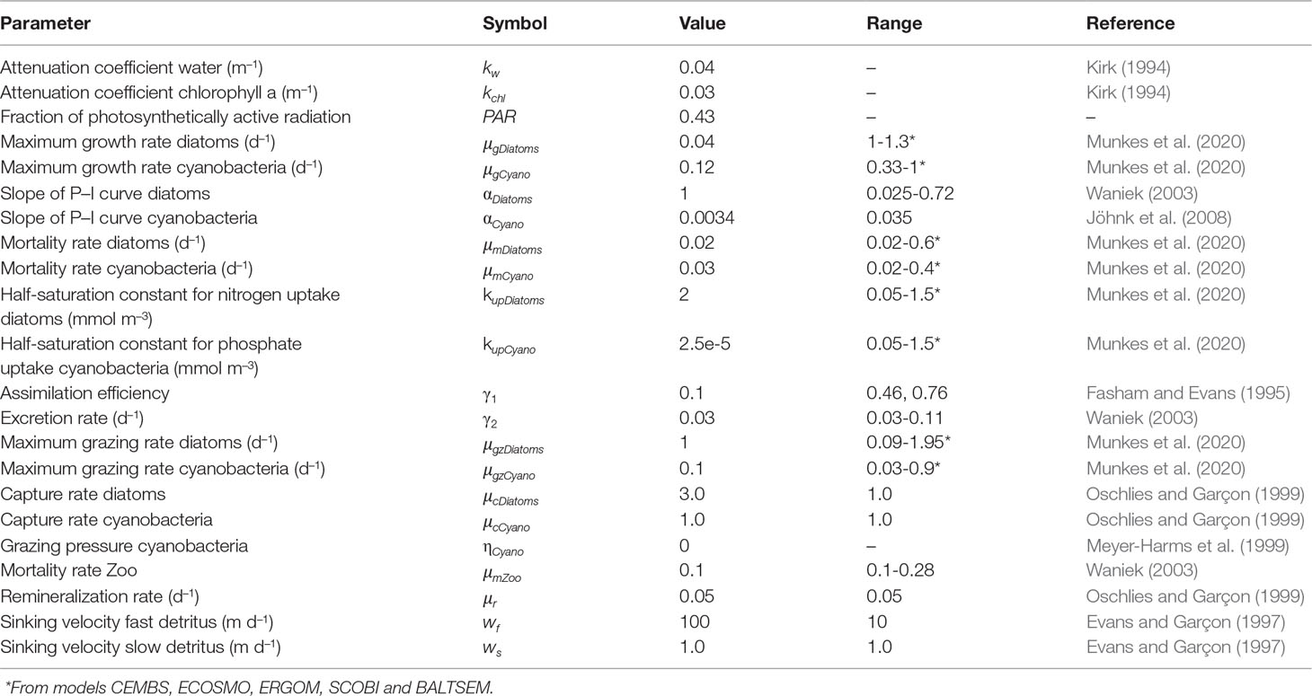
Table 2 List of biological parameters used in the model.
Zooplankton is included in the model for the sole purpose of closing the trophic food chain and to provide the grazing pressure on diatoms, given the limited reliable data regarding zooplankton and their interaction with phytoplankton e.g. in terms of growth, grazing and assimilation rates. Therefore, zooplankton equation does not reflect its life cycle nor the complete interactions of zooplankton with other organisms in the water column. The grazing pressure on diatoms is determined by the maximum grazing rate (μgz) and the catching rate of zooplankton (μc). Thus, the grazing rate is given by the grazing pressure, the assimilation efficiency (γ1), the excretion rate (γ2) and the mortality rate of zooplankton μmZoo.
The remineralization of organic material comprising dead diatoms, cyanobacteria and zooplankton is described by the detritus pool. The detritus pool was split into two groups (fast and slow) based on the sinking speed. Part of the dead organic material may form aggregates that sink rapidly (100 m d–1) while fine organic particles may stay longer in the water column and sink at a slower rate (1 m d-1). The fraction of fast and slow detritus pool within the model is determined by the interaction of detritus with the other model compartments (Figure 2), i.e. it depends on the amount of dead phytoplankton and zooplankton, remineralization rate (μr) and sinking speed (fast (wf) and slow (ws)) in each time step.
The change in nutrient concentration at each time step depends on the remineralization rate of both detritus pools, the excretion rate of zooplankton and phytoplankton uptake during growth. The equations and parameters for the biological state variables are given in Tables 1, 2, respectively. DSi concentrations was assumed to be sufficient during the early phase of the spring bloom when the head-start population had been established (Kremp et al., 2008). At this point, nutrient levels, nutrient ratios or light intensity had only a limited effect on the biomass distribution (Kremp et al., 2008), therefore an aligned Redfield ratio was also assumed.
The ability to fix molecular nitrogen from the atmosphere allows cyanobacteria to circumvent the general summer nitrogen limitation, making phosphorus the primary limiting nutrient for N-fixing cyanobacteria (Walve and Larsson, 2007; Karlson et al., 2015). Furthermore, cyanobacteria studies have highlighted the role of physical forcing and phosphorus over other nutrients during bloom development. Lips and Lips (2008) have shown that blooms for example of Aphanizomenon sp. are initiated by upwelling of phosphorus-rich deeper waters, whereas growth of Nodularia spumigena is mostly related to increases in incoming solar radiation and temperature as well as the ability of this species to make use of regenerated phosphorus pools during the low nutrient concentration periods. Nitrogen fixation by cyanobacteria as well as additional processes involved in bloom formation such as atmospheric nutrient deposition and water column-sediment interaction were not included in the model because they are beyond the scope of this study. Quantification of these processes and parameters such as carbon to chlorophyll a ratio, growth, mortality and remineralization rates is still an active field of research where many questions remain unresolved and valid parametrization for a numerical approach does not exist yet.
One of the limitations of our model is to consider the water column as a rigid parcel of water, where mass and energy exchange takes place through the water column but not with its surroundings. This assumption has implications for all simulated physical, chemical and biological variables, leading to over- or underestimation of these variables and contributing to the model error. In addition, the model was elaborated based on diatoms and cyanobacteria without considering plankton succession or other species such as dinoflagellates that co-occur during the spring bloom because of the limited data to reliable validate each bloom individually and species by species. This simplification may likely affect our results and therefore contribute to the difference observed with other studies and partly observations.
Model Setup and Validation
Vertical profiles of water column temperature and phosphate were taken from the monitoring station TF271 during December 2002 as initial conditions for the model (Table 3). The initial concentration of cyanobacteria and diatoms has a decreasing exponential distribution over depth with a surface value of 0.05 and 0.3 mmol N m–3, respectively. The chlorophyll a concentration was expressed in terms of nitrogen using a chlorophyll a:carbon (Chla:C) ratio of 1:50 and a Redfield ratio between carbon and nitrate (C:N) of 6.6 (Redfield, 1958). The initial concentration of zooplankton was set at 0.1 mmol N m–3 on the surface with a decreasing exponential distribution within a vertical scale of 100 m. An initial concentration of 10–4 mmol N m–3 was used for both detritus pools.
Table 3 Data sets used for model setup and validation.
The model was forced with daily atmospheric reanalysis data from the National Centers for Environmental Prediction (NCEP) (Kalnay et al., 1996). Forcing include air temperature, incoming solar radiation, wind speed, relative humidity and cloud cover (Figure S1). These data provide the basis for calculating the net heat flux and its components (long-wave radiation, sensible and latent heat flux) based on standard bulk formulation (Rahmstorf, 1990) and the estimated temperature at each time step to account for the interaction between the surface and the atmosphere. The model was implemented with a finite differential scheme of 1 m vertical resolution down to the bottom at 240 m and a daily time step. The simulations were done for each year using the same initial conditions and the respective forcing for the year, beginning in 1990 and covering a 30-year period. Thus, the observed variability in spring and summer blooms is driven by the net effect of forcing on the phenology of the bloom. A spin-up time was not included in the simulations.
The results of the model and analyses are restricted to the surface and variables directly related to the development of spring and summer blooms (Figure 3). These variables include nutrients in the form of nitrogen and phosphate (the latter expressed in nitrogen units using the Redfield ratio 1:16 between nitrogen and phosphorus), sea surface temperature, mixed layer depth (MLD), wind speed and net heat flux. The inter-annual variability of diatom and cyanobacteria blooms is compared with observations and satellite data from the study region. Phosphate concentration, sea surface temperature (SST) and net heat flux (Qnet) were also compared with reference data sets in order to evaluate the performance of the model (Table 3).
Figure 3 Model results: (A) cyanobacteria, (B) diatoms, (C) phosphate concentration calculated from nitrogen using N:P ratio, (D) sea surface temperature (SST), (E) mixed layer depth (MLD) and (F) net heat flux (Qnet). The blue and red bars represent periods of diatom and cyanobacteria blooms, respectively.
Phenology Metrics
The threshold criterion was used to identify the phenological dates for spring and summer blooms (Ji et al., 2010). It was defined as an increase in the biomass concentration above a certain level. Wasmund (1997) defined a concentration of 22μg L–1 as a threshold for cyanobacteria blooms in the Baltic Sea. We have taken this value as threshold for spring and summer blooms as it coincides with the biomass at which the onset and decline dates are usually reported for both blooms in the Baltic Sea. However, this threshold strongly influences the results as well as restricts in part the possibility of comparing results with other studies. For this reason we included a trend analysis to make it more robust and comparable with other studies. Overall, the spring bloom begins on day 84 ± 6 ( ± 6 refers to standard deviation) and ends on day 128 ± 9 (Groetsch et al., 2016), while the summer bloom begins on day 168 ± 16 and declines after day 209 ± 13 (Beltran-Perez and Waniek, 2021). The onset of the bloom was defined as the time when the biomass is above the threshold for the first time. The decline of the bloom was set as the time after the biomass maximum reduces to values below the threshold. The duration of the bloom was estimated as the difference between the onset and decline dates of the bloom. The phenology of the bloom was calculated year by year by analyzing the biomass changes between February and May for the spring bloom and between June and August for the summer bloom.
Trend Analyses
The non-parametric Mann-Kendall test (Kendall, 1975) was applied for monotonic downward or upward trends together with the non-parametric Sen method (Sen, 1968) for the slope estimate. This test tolerates outliers and it is independent of the data distribution. This method was applied on the phenological dates identified over the 30-year period for the spring and summer blooms to investigate changes in their occurrence. All calculations and trend analyses were performed in Matlab R2018b. Statistical tests were considered significant with a p-value less than or equal to 0.05.
Results
Inter-Annual Variability
Summer blooms start at the beginning of June and last until the end of August, reaching their maximum concentration in mid-July (Figure 3A). In general, summer blooms have a length of about 3 months and reach a maximum concentration of 10 mmol N m–3. Spring blooms begin on average at the end of March and last until the end of May (Figure 3B) with an average length of roughly 2 months. Their maximum concentrations are observed at the end of April with values around 4 mmol N m–3. Diatoms usually develop a second bloom of lower abundance in autumn that is also captured by the model, but it is outside the scope of this study.
The phosphate concentration shows a cycle where the maximum concentration (around 11 mmol N m–3) is reached during January before the onset of the spring bloom (Figure 3C). The phosphate concentration decreases as the spring bloom is formed, reaching concentrations below 0.5 mmol N m–3 at the beginning of the summer bloom. Phosphate concentration remains low throughout the summer bloom and increases only at the end of the year. The SST shows a pronounced annual cycle with a minimum in mid-February and a maximum in early August (Figure 3D).
The mixed layer depth is directly linked to changes in temperature and mixing intensity, becoming shallower as the solar radiation intensifies and temperature rises (Figure 3E). The shallowest mixed layer depth is reached at around 10 m during the summer bloom, i.e. between June and August. The highest energy gain by the ocean coincides with the end of the spring bloom and the beginning and maximum abundance of the summer bloom (Figure 3F).
The model reproduces the typical annual cycle for spring and summer blooms (Figure 4). The inter-annual variability of both blooms is in good agreement with that derived from observations and satellite data (Figures 4A, B). However, the model underestimates the maximum concentration of the spring bloom and overestimates it for the summer bloom. The pattern of phosphate concentration, SST and net heat flux in Figures 4C–E bears a strong resemblance to the summer bloom pattern, suggesting that the highest cyanobacteria abundance coincides with the minimum in phosphate concentration, high SST and positive net heat flux. The onset of the spring bloom coincides with the maximum phosphate concentration as well as with the increase in SST and net heat flux.
Figure 4 Model results: (A) cyanobacteria, (B) diatoms, (C) phosphate concentration calculated from nitrogen using N:P ratio, (D) sea surface temperature (SST) and (E) net heat flux (Qnet).The circles connected with a solid line represent monthly mean values of the model results (blue) and the reference data sets (red), respectively. The shaded area corresponds to the standard deviation of each variable. Horizontal error bars in (B) represent the standard deviation of bloom occurrence dates. Details of the data sets used as reference are reported in Table 3.
Changes in Phenology of Diatom and Cyanobacteria Blooms
The phenology of the spring and summer blooms is summarized in Tables S1, S2, respectively. The phenology of both blooms is compared with phenological dates derived from observations and satellite data in Figures 5, 6. The onset of the spring bloom coincides with the average onset reported by Groetsch et al. (2016) on day 85 ± 7. The peak and decline dates occur on day 115 ± 6 and 144 ± 5, respectively. Therefore, the length of the bloom is on average 59 ± 4 days. Our phenological dates differ to the observed peak and decline dates by 9 and 17 days, respectively, with the largest differences occurring at the end of the bloom.
Figure 5 Phenological dates for the diatom bloom based on a) model results (1990-2019) and b) observations (2000-2014). In each box, the central red line indicates the median, and the bottom and top edges of the box indicate the 25th and 75th percentiles, respectively. The whiskers extend to the most extreme data points; outlier observations are marked individually using the ‘+’. Details of the data sets used are reported in Table 3.
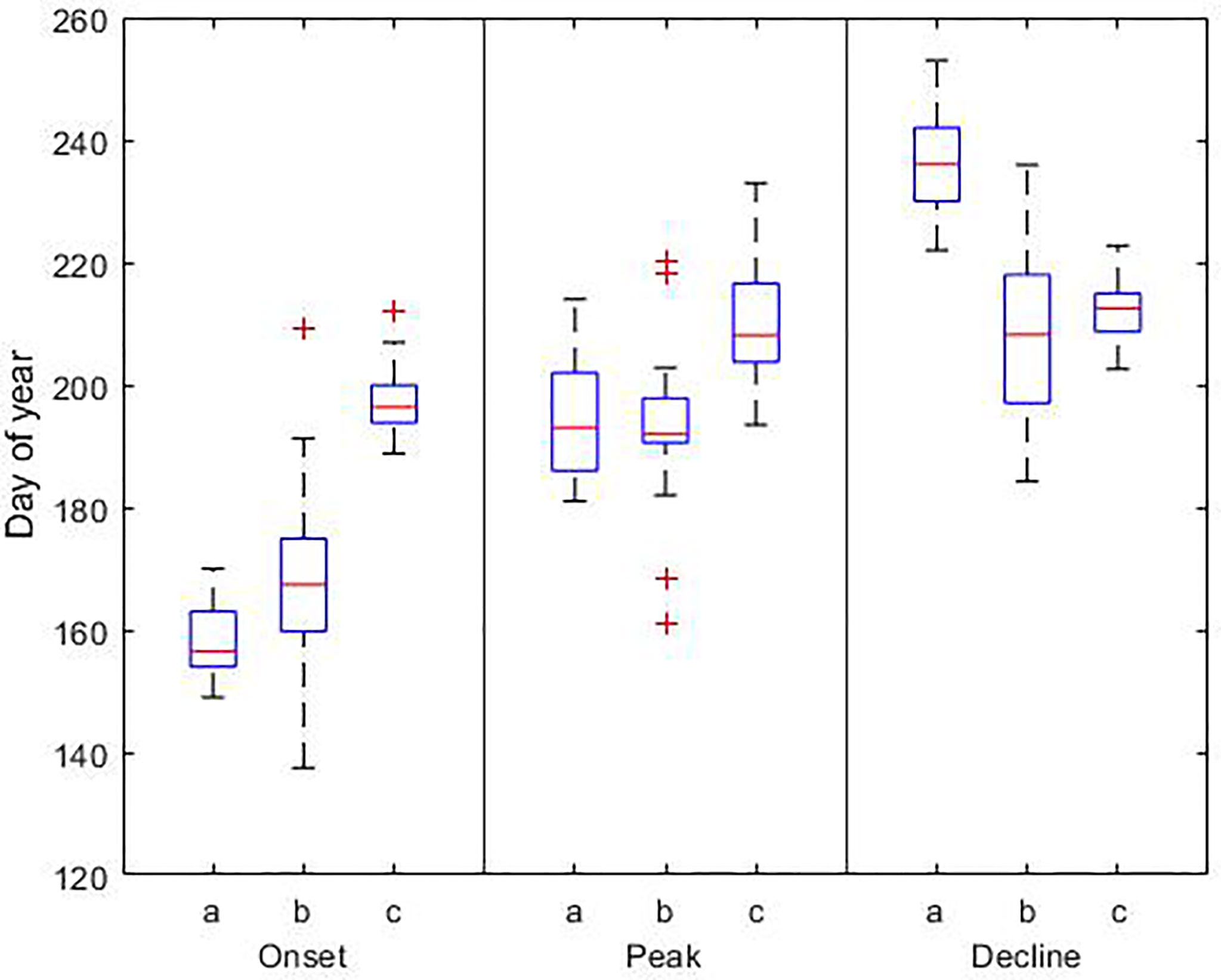
Figure 6 Phenological dates for the cyanobacteria bloom based on a) model results (1990-2019), b) observations (1990-2017), and c) satellite data (1998-2015). In each box, the central red line indicates the median, and the bottom and top edges of the box indicate the 25th and 75th percentiles, respectively. The whiskers extend to the most extreme data points; outlier observations are marked individually using the ‘+’. Details of the data sets used are reported in Table 3.
Based on the results of the model, the summer bloom starts on day 158 ± 5, reaches its maximum biomass on day 194 ± 9 and declines on day 237 ± 8. On average the bloom lasts 79 ± 9 days. Similar to the results for the spring bloom, there is a discrepancy between our results, observations and satellite data. The bloom begins 9 and 38 days earlier than in observations and satellite data, respectively. The occurrence of the maximum coincides with in situ observations, but not with satellite data. The maximum occurs on day 194 in the model and observations, but 15 days later in satellite data. The largest difference is at the end of the bloom. According to our results the bloom ends on day 237, but using observations and satellite data it ends 27 and 22 days earlier, respectively.
The inter-annual variability of the summer bloom showed significant temporal changes (p-value < 0.05) in the onset and length of the bloom (Figure 7). Summer blooms occur 9 days earlier, starting on day 152 in 2019 instead of day 161 in 1990 in the Gotland Basin. They last 15 days longer, increasing their length from 72 days in 1990 to 87 days in 2019. However, a longer bloom did not necessarily lead to a higher abundance of cyanobacteria. No temporal changes were found for the peak or decline dates of the summer bloom. The spring bloom showed no statistically significant changes in phenology and abundance over the 30-year period.
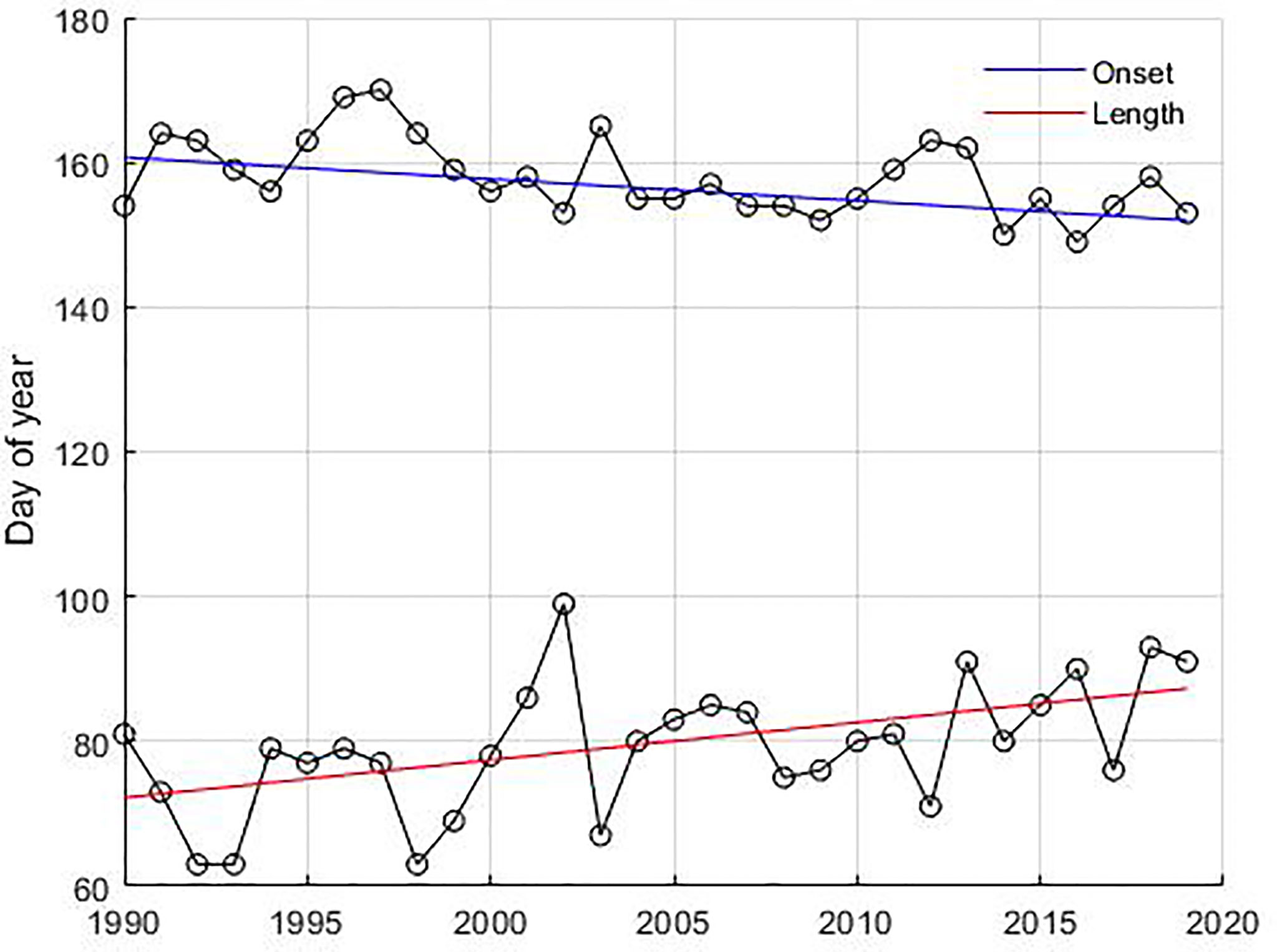
Figure 7 Temporal change in the phenological dates of cyanobacteria blooms. The circles connected with a black solid line represent onset dates and length of the bloom, respectively. The slope of the curve for the onset dates (blue line) and length ofthe bloom (red line) was estimated using the Mann-Kendall test with the non-parametric Sen method using 95% significance level.
Effect of Environmental Variables on Bloom Phenology
To emphasize the changes in spring and summer blooms occurrence and their relationship with SST, wind and net heat flux we have calculated the anomalies for SST, wind and net heat flux with respect to each bloom period (Figures S2, S3). We selected years with the higher positive and negative anomalies for each variable during the development of each bloom, i.e. during February and May for the spring bloom and June and August for the summer bloom (Tables 4, 5 and Figures 8, 9). During the spring bloom, the SST was around 1.5°C higher than average in 1990, 2008 and 2015 and lower roughly 2 °C in 1996, 2003 and 2010 (Figure S2A). Summer blooms were observed at SST roughly 0.5°C higher than average in 1990, 2002 and 2018 and 0.5°C lower in 1996, 2015 and 2017 (Figure S3A). SST anomalies indicate that the spring and summer seasons were warmer than average during 1990, while colder during 1996. In 2015 a warm spring followed by a cold summer was observed, both seasons were characterized by particularly strong winds (Figures S2B, S3B). Winds 1 ms−1 higher than average were found during spring blooms in 1997, 2015 and 2019. The stronger winds during summer blooms are roughly 0.5 ms−1 higher than average and occurred in 1998, 2004 and 2015. The response of the spring bloom changes over time but a strong relationship with the heat exchange between atmosphere and surface ocean was not observed (Figure S2C). On the contrary, summer blooms are generally observed to coincide with positive net heat flux anomalies (high energy gain) and negative wind anomalies (calm wind conditions), which are linked to higher water column stability (Figure S3C).
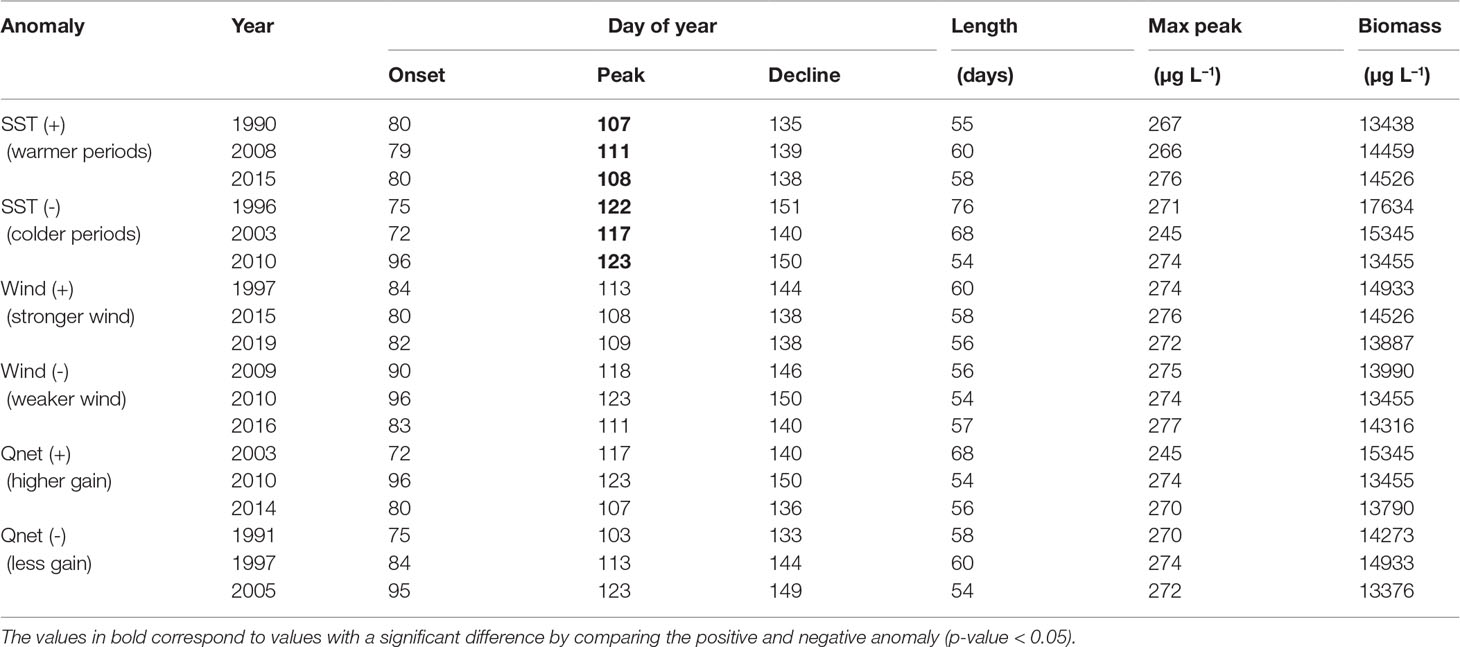
Table 4 Diatoms biomass integrated over the bloom period (February-May) calculated for the periods with the highest (+) and smallest (-) anomalies in SST, wind and net heat flux (Qnet).
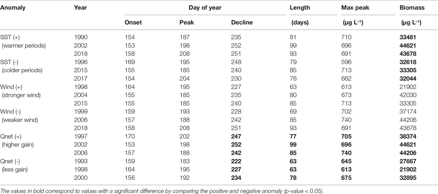
Table 5 Cyanobacteria biomass integrated over the bloom period (June-August) calculated for the periods with the highest (+) and smallest (-) anomalies in SST, wind and net heat flux (Qnet).
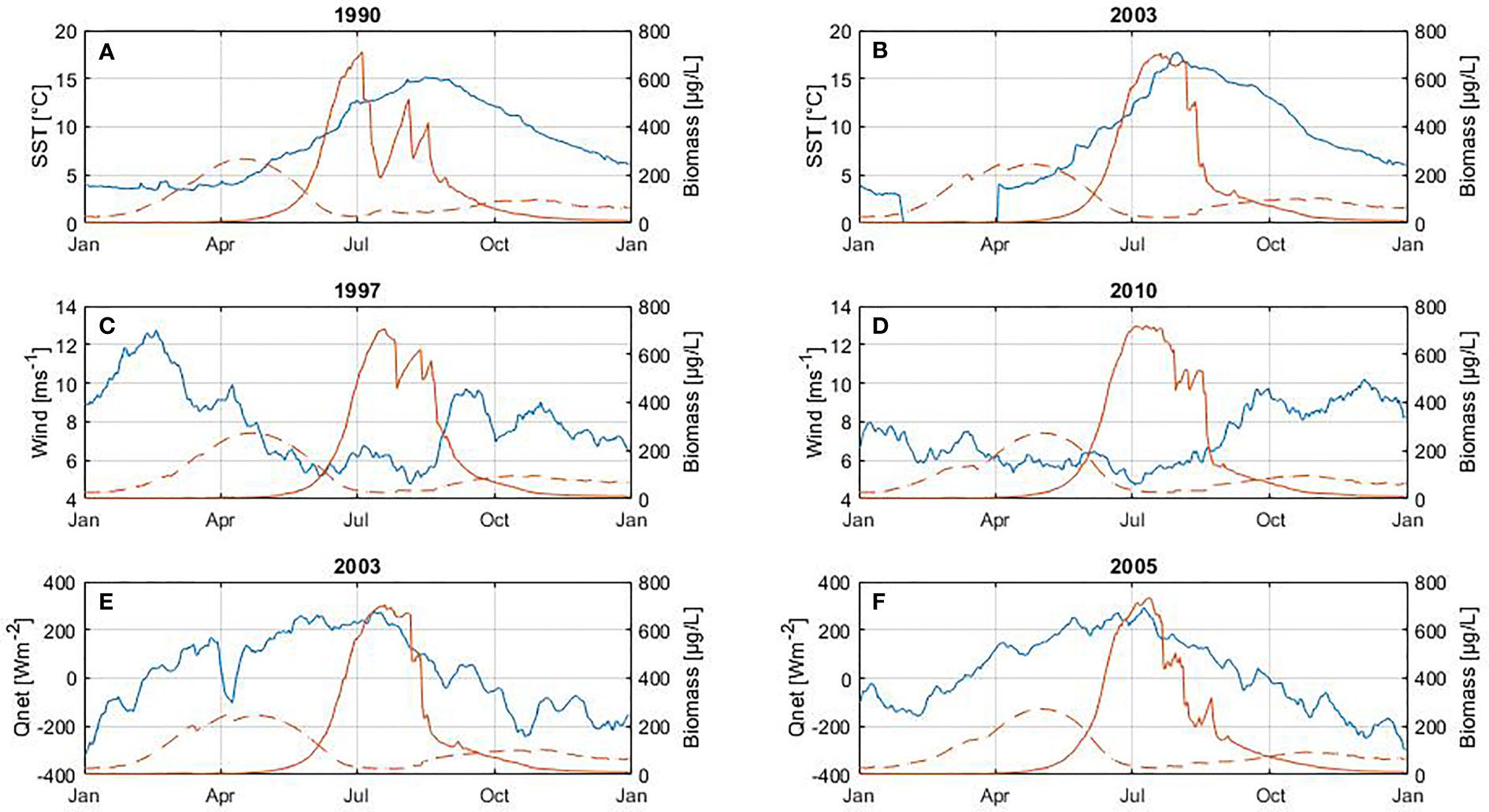
Figure 8 Influence of SST (A, B), wind (C, D) and net heat flux (E, F) on diatom biomass (between February and May). At the top of each plot is shown the year with the highest positive anomalies (left panel) and negative anomalies (right panel) for each variable. The blue line corresponds to the variable (left axes) and the red line to biomass (right axes) of diatoms (dashed line) and cyanobacteria (solid line). The cyanobacteria bloom is included only to illustrate its inter-annual cycle.
There is a statistically significant change in the occurrence of the spring bloom with respect to SST (Table 4). During warmer periods the peak of the bloom occurs on average on day 109, while in cooler periods it occurs on day 121. As a result, spring blooms reach maximum biomass 12 days earlier in warmer periods. No further significant changes in phenology or abundance were found for the spring bloom.
A significant difference in cyanobacteria biomass is found when comparing positive and negative SST anomalies (Table 5). Cyanobacteria blooms develop higher biomass during warmer periods than during colder periods. There is also a significant difference in the biomass, decline dates, length and maximum peak of the summer bloom when comparing positive and negative net heat flux anomalies. Thus, a higher energy gain (positive net heat flux) by the ocean leads to a bloom with higher abundance and maximum peak as well as the extension of the bloom by delaying its end by around 19 days.
The highest cyanobacteria abundance coincides with calm wind conditions (Figure 9), however no statistically significant difference was found between the occurrence of the bloom and calm wind (p-value > 0.05, Table 5). Similarly, the spring bloom did not show a statistically significant difference with respect to the wind strength (Table 4).
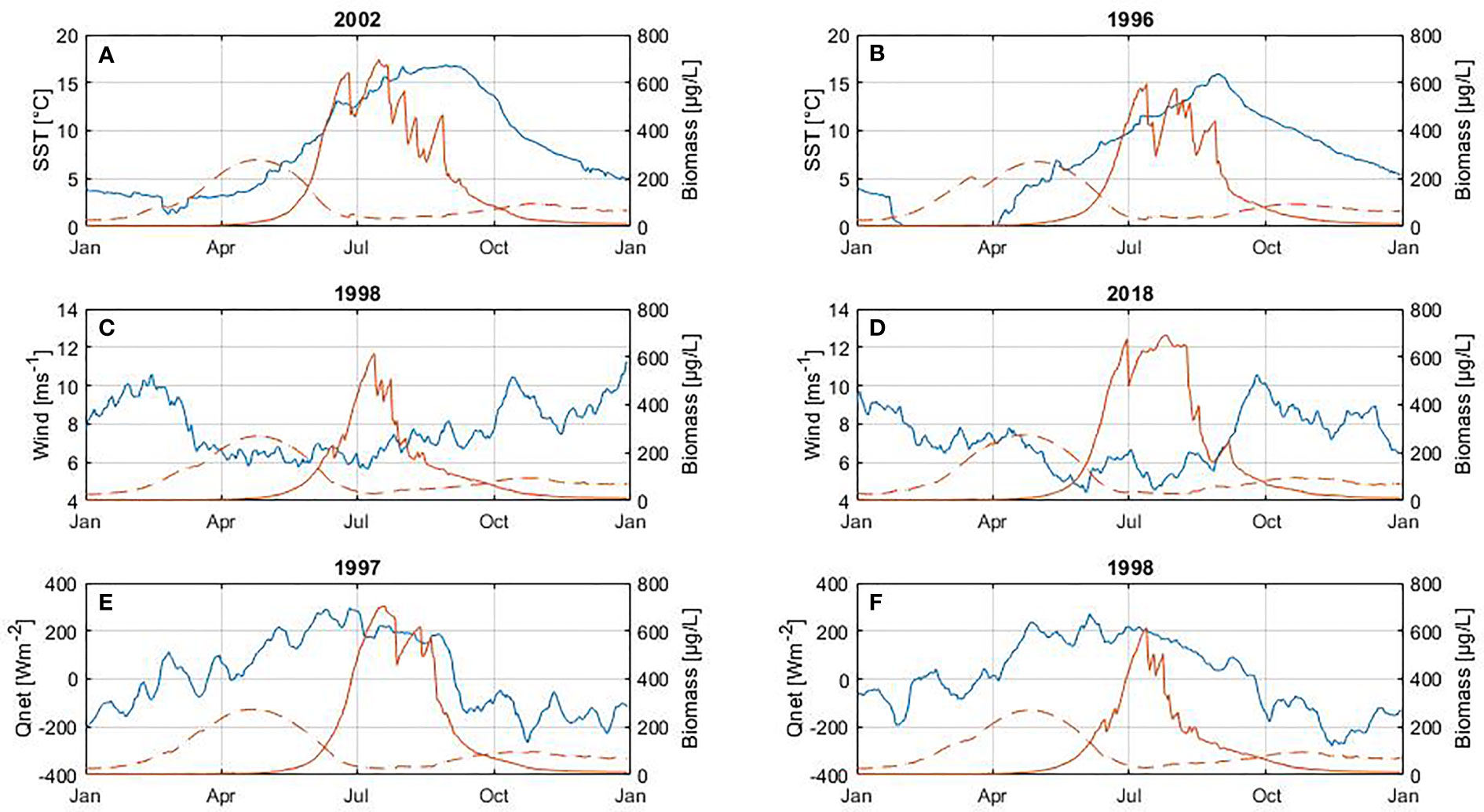
Figure 9 Influence of SST (A, B), wind (C, D) and net heat flux (E, F) on cyanobacteria biomass (between June and August). At the top of each plot is shown the year with the highest positive anomalies (left panel) and negative anomalies (right panel) foreach variable. The blue line corresponds to the variable (left axes) and the red line to biomass (right axes) of diatoms (dashed line) and cyanobacteria (solid line). The diatom bloom is included only to illustrate its inter-annual cycle.
Discussion
Inter-annual and temporal variability of spring and summer blooms in the Gotland Basin has been described by Wasmund and Uhlig (2003); Janssen et al. (2004); Wasmund et al. (2011), but the phenology and response of these blooms to changing environmental conditions have been studied less extensively and remain unclear (Kahru and Elmgren, 2014; Groetsch et al., 2016; Kahru et al., 2016). Our results show that the occurrence of spring and summer blooms is affected differently by changes in SST, wind and net heat flux. The mixing in the water column is largely related to density changes (through buoyancy forcing by net heat flux) that drive the variability of the mixed layer (Figures 3D–F).
The onset of the spring bloom is consistent with the findings of Groetsch et al. (2016), who estimated the phenology of the spring bloom from a 15-year time series (2000–2014) of ship-of-opportunity chlorophyll a fluorescence observations for different regions in the Baltic Sea. However, in our results the average peak and decline dates occur later than in the aforementioned study. The use of a fixed threshold in our study (22 μg L–1) instead of the 10th and 90th percentiles before and after the bloom peak used by Groetsch et al. (2016) resulted in a later occurrence of the peak and decline dates, as more time is allowed for spring and summer blooms to exceed the specified threshold value. The discrepancy between both studies may be explained by the method used to quantify the biomass, and the threshold criteria used for the computation of the phenological dates. The definition of the threshold at which bloom begins or ends differs between studies, a trend analysis is more robust and therefore it was used to compare with other studies.
Earlier spring blooms have previously been reported for the Baltic Sea (Fleming and Kaitala, 2006; Klais et al., 2013). Our study showed that higher temperatures cause the spring bloom to peak earlier, but this was not observed over the 30-year period, i.e. changes in the timing of the peak occurrence over the 30-year period were not statistically significant (p-value > 0.05). Wasmund et al. (2011) also reported that there is no trend for the spring bloom in the eastern Baltic Sea during the period 1979 to 2005. However, other studies have found that spring blooms tend to develop earlier and less intense. Kahru et al. (2016) showed an advance of the growth season at a mean rate of 1.6 days per year for the spring bloom in the entire Baltic Sea. Groetsch et al. (2016) found a positive trend in the bloom length of 1 ± 0.20 day per year and a negative trend in chlorophyll a maximum of 0.31 ± 0.10 mg m–3 per year for the spring bloom over the period 2000 to 2014, attributing it to the gradual reduction of nutrients load in the Baltic Sea. Long-term data sets from 1979 to 2011 also showed a decrease in diatom abundance during the spring bloom in the Baltic Proper (Wasmund and Uhlig, 2003; Wasmund et al., 2013).
The phenology of the spring bloom seems to be affected only by SST (Figure 8 and Table 4), which result in the spring bloom reaching its maximum abundance earlier. Higher temperatures favor the spring bloom by intensifying stratification, which increases light in a shallow mixed layer following the critical depth hypothesis (Sverdrup, 1953), as Sommer et al. (2012) confirmed using several temperatures and light levels in a series of mesocosm experiments. Light is necessary for phytoplankton photosynthesis and growth, while temperature influences growth rates and stratification. Wind has a dual effect on the bloom. On the one hand, strong winds induce mixing that favors redistribution of the resting stages of diatoms and nutrients in the water column (Hjerne et al., 2019). On the other hand, calm wind conditions are associated with lower energy losses or energy gain on the surface, increasing temperature and stratification of the water column (Wasmund et al., 1998; Wasmund and Uhlig, 2003; Wasmund et al., 2013). Therefore, according to our results and those from other studies (Groetsch et al., Reynolds et al., 1984; Spilling and Markager, 2008; Sommer et al., 2012; Wasmund et al., 2013), the spring bloom is favored by the ability of diatoms to proliferate despite strong wind (Figure 3B and Figure S1C) following Margalef’s mandala (Margalef, 1978), the availability of nutrients during the first months of the year (Figures 3B, C) and the increasing amount of light as well (Figure 3B and Figure S1B) following Sverdrup’s hypothesis (Sverdrup, 1953).
We found evidence that the occurrence of earlier maximum abundance in the spring bloom was related to warm weather conditions (Figure 8 and Table 4). Changes in the spring bloom phenology may influence the survival of higher trophic levels due to variations in timing of food availability (match-mismatch hypothesis) (Smith and Hollibaugh, 1993; Winder and Schindler, 2004), i.e. the energy and carbon transfer from primary production to pelagic fish production (Sommer et al., 2012). A shift in the spring bloom may inhibit the survival of zooplankton and fish, affecting the recruitment of larvae as larval spawning continues to match the original timing of the bloom prior to changes (Cole, 2014; Gittings et al., 2018). As a result, potential negative impacts can be expected on the Baltic Sea ecosystem if changes in the phenology of phytoplankton blooms continue in conjunction with current changes in the environment.
The occurrence of the maximum cyanobacteria abundance in the model coincides with in situ observations but not with that estimated based on satellite data. There are, however, differences in the onset and decline of the bloom probably due to the definition of the threshold at which species abundance exceeds normal values in the water. The lack of consensus on the definition of thresholds in phenological studies makes it difficult to compare the results between them. In fact, using thresholds defined on a percentile basis like in other studies, our results deviate from the time at which cyanobacteria blooms usually occur in the Baltic Sea (i.e. between June and August). Additionally, to the uncertainty surrounding the defined threshold at which the bloom develops, it is not surprising that our results vary from the phenological dates identified based on satellite imagery. Remote sensing is able to detect blooms only when strong surface aggregations are formed, which usually occurs at an advanced bloom stage and directly related with the cyanobacteria species Nodularia spumigena, the only species of the summer bloom in the Baltic Sea that forms dense surface accumulations. Nodularia spumigena is a co-dominant cyanobacteria species in the Baltic Sea, the other co-dominant species, Aphanizomenon sp. and Dolichospermum spp., although both are present during the bloom, these species are typically found at the subsurface and therefore not specifically detected through satellites (Kahru and Elmgren, 2014; Eigemann et al., 2018; Kahru et al., 2020).
Until now, there has been no consensus on whether cyanobacteria blooms will increase or decrease in the future (Wasmund and Uhlig, 2003; Kahru and Elmgren, 2014; Kahru et al., 2016; Meier et al., 2019). Our results support the findings of other studies which point to summer blooms starting earlier and lasting longer. We found that the summer bloom is occurring 0.3 days earlier each year and extending its length by 0.5 days per year. Kahru and Elmgren (2014) found progressively earlier accumulations of cyanobacteria in summer by approximately 0.6 days per year over a 35-year period. Kahru et al. (2016) also found trends towards an earlier start of the spring and summer blooms. Contrary to these results, Wasmund and Uhlig (2003) found no indication that cyanobacteria blooms have increased during the period 1979-1999, even if there is a tendency to decrease in some basins of the Baltic Sea. On the one hand, observations from satellites in the Baltic Sea are based on chlorophyll a and focused on specific species of cyanobacteria such as Nodularia spumigena, which forms dense surface accumulations (Kahru and Elmgren, 2014; Kahru et al., 2020). On the other hand, in situ observations of phytoplankton biomass are usually integrated over the water column and the frequency of observations is limited in time and space, which in case of blooms may lead to differences in the estimated biomass and phenology of the bloom when compared to other studies even during similar periods of time and locations. Although the results from observations and satellites may vary, they are the closest approximations available to identify and validate bloom phenology as long-term in situ data sets and studies defining bloom phenology are still scarce. Therefore, they have been used in this study and compared despite their significant differences, being aware of the limitations of both approaches (Kahru and Elmgren, 2014; Gittings et al., 2019).
Overall, cyanobacteria species are able to uptake a large amount of nutrients and store them to maintain growth and survive for days (Kanoshina et al., 2003; Flores and Herrero, 2005). Therefore, cyanobacteria blooms are able to develop under depleted phosphorus (limiting nutrient) conditions (Figures 3C, 4C) (Wasmund, 1997; Lignell et al., 2003). Cyanobacteria abundance is coupled with SST at seasonal and inter-annual time scales (Figures 3, 4), signifying that warmer periods favor cyanobacteria growth (Table 5) as other studies have also indicated (Hense et al., 2013). Warm years characterised by higher cyanobacteria biomass (e.g. 1990, 2002 and 2018) coincide with a shallower MLD and stratified water column (Figures 3A, D–F).
The change in the length of the summer bloom was not observed in connection with temperature, but rather with net heat flux (Figure 9 and Table 5). For years with a strong heat gain during summertime such as 1997, 2002, 2006 the bloom extends on average 19 days compared to years with lower heat gain such as 1993, 1998, 2000, which is in agreement with the trend observed for the summer bloom to extend its length over the entire 30-year period. The energy gain by the water column contributes significantly to the increase in bloom abundance by intensifying stratification. Cyanobacteria blooms do not tolerate turbulence so calm wind conditions and a strongly stratified water column favor their development resulting in longer blooms (Table 5). These results are supported by Beltran-Perez and Waniek (2021) who demonstrated that the phenology of cyanobacteria blooms is explained by the energy exchange between the atmosphere and the ocean. Only a few studies have highlighted the role of energy exchange at the ocean-atmosphere interface that regulates mixing in the water column in the context of phenology studies so far (Gittings et al., 2018; Beltran-Perez and Waniek, 2021).
Our results showed that changes in wind strength do not lead to changes in bloom phenology as Kahru et al. (2020) also indicated for cyanobacteria accumulations and wind on a decadal and inter-annual time scale. Calm wind may have an influence on the development of the bloom as reported by other studies (Wasmund, 1997; Kanoshina et al., 2003), but in this study, if there is such an influence, it was not statistically significant.
Water temperature has been increasing during the past 100 years and it is projected to further increase between 1.1°C to 3.2 °C by the end of this century in the Baltic Sea (HELCOM/Baltic Earth, 2021). Higher temperatures intensify stratification and therefore favor the occurrence of summer blooms. Our results support the occurrence of earlier and longer blooms, but there is much uncertainty about whether cyanobacteria blooms may increase in the future. The observed changes in the phenology of summer blooms and their relationship with global warming suggest that cyanobacteria blooms will remain a major concern for the Baltic Sea. They may accelerate eutrophication and oxygen depletion in the water column (Larsson et al., 1985; Wasmund, 1997; Janssen et al., 2004) and have stronger impacts on fishing and recreational use of coastal waters (Paerl and Huisman, 2009; Neil et al., 2012), as many species of cyanobacteria produce toxins. Alterations in the food web are also expected as the efficiency of energy transfer to higher trophic levels may reduce due to the poor food quality of cyanobacteria for grazers, depending on the availability of other sources of food and the type of zooplankton and cyanobacteria species (Meyer-Harms et al., 1999; Ger et al., 2016; Munkes et al., 2020).
The Baltic Sea is one of the most intensively monitored seas in the world; however, its observations are not sufficient to determine in detail phytoplankton phenology. Coupling of data on species-specific life cycles and succession to environment conditions (e.g. nutrient ratios, light, temperature), other organisms (e.g. prey, predators, competitors), as well as to process-based models appears necessary to explain the timing and intensity of spring and summer blooms in the study area and neighboring habitats. A simple, one-dimensional, coupled physical-biological model based on the basic equations governing bloom formation was able to reproduce the development of the bloom with reliable results and showed the effect of forcing on phenology of both blooms. Therefore, the use of models provides a solid basis for testing phytoplankton bloom hypothesis as observations are limited and may not necessarily cover the bloom development because samples are usually taken during specific very limited time periods and locations.
Conclusions
Overall, the model reproduces the inter-annual and temporal variability of spring and summer blooms considering the constraints and limitations of the model. On average the spring bloom started on day 85, reached its maximum on day 115 and declined on day 144. Warmer periods cause the spring bloom to peak earlier, but no statistically significant trend was found for the spring bloom over the period 1990 to 2019. The summer bloom started on day 158, had its maximum on day 194 and declined after day 237. Summer blooms were found to occur 9 days earlier and last 15 days longer over a 30 year period. Our results differ from results of other phenological studies mainly at the end of both blooms. More phenological studies are needed to define with certainty the changes in the occurrence of spring and summer blooms over time.
The influence of environmental variables such as sea surface temperature, wind and net heat flux on the occurrence of spring and summer blooms was confirmed. It was observed that warmer periods affect the spring and summer blooms differently. The spring bloom reaches its maximum earlier whereas the summer bloom increases its abundance. The heat exchange between the water and the atmosphere also had a significant influence on the summer bloom. A stronger heat gain delays the end of the summer bloom, increases its length, abundance and leads to higher biomass maxima due to greater water column stability. Overall, summer blooms are more sensitive to changes in the environment than spring blooms, therefore summer blooms are expected to react more quickly to the changes generated by climate change in the Baltic Sea. However, minor changes in the spring bloom may significantly affect the quantity and quality of food reaching the seafloor, leading to alterations in the entire ecosystem. Further research is needed to follow in detail the development of phytoplankton blooms and succession changes that may occur in response to changes in the environment.
Process-based models provide process- and feedback-understanding, since observations alone are usually limited in time and space. However, parameterization remains one of the main sources of uncertainty in all models. Our one-dimensional model provides reliable insight into the inter-annual variability of spring and summer blooms and the effect of forcing on phenology of both blooms considering model limitations and assumptions. The threshold method showed the best results with respect to the metrics used to identify bloom phenology. However, phytoplankton response to changes and threshold values is far from universal and depends on species-by-species and site-by-site basis (Hallegraeff et al., 2021). There is an urgent need defining a threshold, which should full fill the following criteria: 1) be valid for different blooms, 2) be applicable to blooms around the globe and 3) be set up based on observations. Right now the only threshold that meets partly these characteristics corresponds to 22 μgL–1(2.7 mmol N m–3). It was previously reported by Wasmund (1997) in the identification of cyanobacteria bloom in the Baltic Sea, but its general applicability to define bloom phenology was not yet tested, as far as we are aware of.
More complex models or techniques such as statistical models, genetic algorithm and machine learning need to be explored in more detail in order to improve the modeling of phytoplankton blooms and thus their phenology. Overall, more frequent observations of e.g. growth and mortality rates, isotope markers or other physiological indicators (e.g. genomics, transcriptomics, proteomics, metabolomics) provide a broader understanding of bloom phenology and longer data sets for model initialization and validation, data sets needed to improve the performance of our and other models.
Data Availability Statement
Publicly available data sets were used in this study. The data can be found here: https://odin2.io-warnemuende.de/, https://sharkweb.smhi.se/hamta-data/, https://www.smhi.se/data/oceanografi/ladda-ner-oceanografiska-observationer/ and https://psl.noaa.gov/data/gridded/data.ncep.reanalysis.surfaceflux.html.
Resource Identification Initiative:
MATLAB, RRID: SCR_001622, NCBITaxon: 2836, NCBITaxin: 2864, NCBITaxon: 1117.
Author Contributions
JW provided the initial version of the model and supervised the study. OB-P extended the model to other phytoplankton species, calibrated and validated the model outputs, analyzed the data, produced the figures and wrote the manuscript. JW and OB-P contributed to the interpretation of results, the discussion and subsequent edits of the manuscript. Both authors have read and agreed to the published version of the manuscript.
Funding
Funding granted by the DAAD program: Research Grants - Doctoral Programmes in Germany 2018/19.
Conflict of Interest
The authors declare that the research was conducted in the absence of any commercial or financial relationship that could be construed as a potential conflict of interest.
Publisher’s Note
All claims expressed in this article are solely those of the authors and do not necessarily represent those of their affiliated organizations, or those of the publisher, the editors and the reviewers. Any product that may be evaluated in this article, or claim that may be made by its manufacturer, is not guaranteed or endorsed by the publisher.
Acknowledgments
The authors thank the DAAD for the funding granted and the Leibniz Institute for Baltic Sea Research (IOW) for the facilities, data access, and support provided during the writing of the manuscript. We want to acknowledge the anonymous reviewers for their constructive comments that helped us to improve the quality of the manuscript.
Supplementary Material
The Supplementary Material for this article can be found online at: https://www.frontiersin.org/articles/10.3389/fmars.2022.928633/full#supplementary-material
References
Beckmann A., Hense I. (2007). Beneath the surface: Characteristics of Oceanic Ecosystems Under Weak Mixing Conditions - A Theoretical Investigation. Prog. Oceanogr. 75, 771–796. doi: 10.1016/j.pocean.2007.09.002
Beltran-Perez O. D., Waniek J. J. (2021). Environmental window of cyanobacteria bloom occurrence. J. Mar. Syst. 224, 103618. doi: 10.1016/j.jmarsys.2021.103618
Bianchi T. S., Engelhaupt E., Westman P., Andrén T., Rolff C., Elmgren R. (2000). Cyanobacterial Blooms in the Baltic Sea: Natural or Human-Induced? Limnol. Oceanogr. 45, 716–726. doi: 10.4319/lo.2000.45.3.0716
Breitburg D., Levin L. A., Oschlies A., Grégoire M., Chavez F. P., Conley D. J., et al. (2018). Declining Oxygen In the Global Ocean and Coastal Waters. Science 359. doi: 10.1126/science.aam7240. (80), 1–11.
Carey C. C., Ibelings B. W., Hoffmann E. P., Hamilton D. P., Brookes J. D. (2012). Eco-Physiological Adaptations That Favour Freshwater Cyanobacteria in a Changing Climate. Water Res. 46, 1394–1407. doi: 10.1016/J.WATRES.2011.12.016
Cole H. S. (2014). The Natural Variability and Climate Change Response in Phytoplankton (UK: University of Southampton). Doctoral Dissertation.
Daewel U., Schrum C. (2017). Low-Frequency Variability in North Sea and Baltic Sea Identified Through Simulations with the 3-D Coupled Physical-Biogeochemical Model ECOSMO. Earth Syst. Dyn. 8, 801–815. doi: 10.5194/esd-8-801-2017
Dzierzbicka-Głowacka L., Janecki M., Nowicki A., Jakacki J. (2013). Activation of the Operational Ecohydrodynamic Model (3D CEMBS) - The Ecosystem Module. Oceanologia 55, 543–572. doi: 10.5697/oc.55-3.543
Eigemann F., Schwartke M., Schulz-Vogt H. (2018). Niche Separation of Baltic Sea Cyanobacteria During Bloom Events by Species Interactions and Autecological Preferences. Harmful Algae 72, 65–73. doi: 10.1016/j.hal.2018.01.001
Evans G., Garçon V. C. (1997). “One-Dimensional Models of Water Column Biogeochemistry,” in JGOFS Rep. 23/97 (Bergen, Norway: Scientific Committee on Oceanic Research), 4–7.
Fasham M. J., Evans G. T. (1995). The Use of Optimization Techniques to Model Marine Ecosystem Dynamics at the JGOFS Station at 47° N 20° W. Philos. Trans. R. Soc London. Ser. B Biol. Sci. 348, 203–209. doi: 10.1098/RSTB.1995.0062
Fleming V., Kaitala S. (2006). Phytoplankton Spring Bloom Intensity Index for the Baltic Sea Estimated for the Years 1992 to 2004. Hydrobiologia 554, 57–65. doi: 10.1007/s10750-005-1006-7
Flores E., Herrero A. (2005). Nitrogen Assimilation and Nitrogen Control in Cyanobacteria. Biochem. Soc Trans. 33, 164–167. doi: 10.1042/BST0330164
Ger K. A., Urrutia-Cordero P., Frost P. C., Hansson L. A., Sarnelle O., Wilson A. E., et al. (2016). The Interaction Between Cyanobacteria and Zooplankton in a More Eutrophic World. Harmful Algae 54, 128–144. doi: 10.1016/j.hal.2015.12.005
Gittings J. A., Raitsos D. E., Kheireddine M., Racault M. F., Claustre H., Hoteit I. (2019). Evaluating Tropical Phytoplankton Phenology Metrics Using Contemporary Tools. Sci. Rep. 9, 1–9. doi: 10.1038/s41598-018-37370-4
Gittings J. A., Raitsos D. E., Krokos G., Hoteit I. (2018). Impacts of Warming on Phytoplankton Abundance and Phenology in a Typical Tropical Marine Ecosystem. Sci. Rep. 8, 1–12. doi: 10.1038/s41598-018-20560-5
Groetsch P. M., Simis S. G., Eleveld M. A., Peters S. W. (2016). Spring Blooms in the Baltic Sea have Weakened but Lengthened from 2000 to 2014. Biogeosciences 13, 4959–4973. doi: 10.5194/bg-13-4959-2016
Gustafsson E. (2012). Modelled Long-Term Development of Hypoxic Area and Nutrient Pools in the Baltic Proper. J. Mar. Syst. 94, 120–134. doi: 10.1016/j.jmarsys.2011.11.012
Hallegraeff G. M., Anderson D. M., Belin C., Bottein M.-Y. D., Bresnan E., Chinain M., et al. (2021). Perceived Global Increase in Algal Blooms is Attributable to Intensified Monitoring and Emerging Bloom Impacts ( Commun). doi: 10.1038/s43247-021-00178-8
Hashioka T., Sakamoto T. T., Yamanaka Y. (2009). Potential Impact of Global warming on North Pacific spring blooms projected by an eddy-permitting 3-D Ocean Ecosystem Model. Geophys. Res. Lett. 36, 1–5. doi: 10.1029/2009GL038912
HELCOM/Baltic Earth (2021). “Climate Change in the Baltic Sea,” in 2021 Fact Sheet. Tech. rep. (Helsinki, Finland: Helsinki Commission - HELCOM)
HELCOM (2012). Manual for Marine Monitoring in the COMBINE Programme of HELCOM (Helsinki, Finland:Helsinki Commission - Baltic Marine Environment Protection Commission).
Hense I., Burchard H. (2010). Modelling Cyanobacteria in Shallow Coastal Seas. Ecol. Modell. 221, 238–244. doi: 10.1016/j.ecolmodel.2009.09.006
Hense I., Meier H. E., Sonntag S. (2013). Projected Climate Change Impact on Baltic Sea Cyanobacteria: Climate Change Impact on Cyanobacteria. Clim. Change 119, 391–406. doi: 10.1007/s10584-013-0702-y
Henson S. A., Dunne J. P., Sarmiento J. L. (2009). Decadal Variability in North Atlantic Phytoplankton Blooms. J. Geophys. Res. Ocean. 114, 1–11. doi: 10.1029/2008JC005139
Hjerne O., Hajdu S., Larsson U., Downing A., Winder M. (2019). Climate Driven Changes in Timing, Composition and Size of the Baltic Sea Phytoplankton Spring Bloom. Front. Mar. Sci. 6. doi: 10.3389/fmars.2019.00482
Janssen F., Neumann T., Schmidt M. (2004). Inter-annual Variability in Cyanobacteria Blooms in the Baltic Sea Controlled by Wintertime Hydrographic Conditions. Mar. Ecol. Prog. Ser. 275, 59–68. doi: 10.3354/meps275059
Ji R., Davis C. S., Chen C., Townsend D. W., Mountain D. G., Beardsley R. C. (2008). Modeling the Influence of Low-Salinity Water Inflow on Winter-Spring Phytoplankton Dynamics in the Nova Scotian Shelf-Gulf of Maine Region. J. Plankton Res. 30, 1399–1416. doi: 10.1029/2007GL032010
Ji R., Edwards M., MacKas D. L., Runge J. A., Thomas A. C. (2010). Marine Plankton Phenology and Life History in a Changing Climate: Current Research and Future Directions. J. Plankton Res. 32, 1355–1368. doi: 10.1093/plankt/fbq062
Jöhnk K. D., Huisman J., Sharples J., Sommeijer B., Visser P. M., Stroom J. M. (2008). Summer Heatwaves Promote Blooms of Harmful Cyanobacteria. Glob. Change Biol. 14, 495–512. doi: 10.1111/j.1365-2486.2007.01510.x
Kahru M., Elmgren R. (2014). Multidecadal Time Series of Satellite-Detected Accumulations of Cyanobacteria in the Baltic Sea. Biogeosciences 11, 3619–3633. doi: 10.5194/bg-11-3619-2014
Kahru M., Elmgren R., Kaiser J., Wasmund N., Savchuk O. (2020). Cyanobacterial Blooms in the Baltic Sea: Correlations with Environmental Factors. Harmful Algae 92, 101739. doi: 10.1016/j.hal.2019.101739
Kahru M., Elmgren R., Savchuk O. P. (2016). Changing Seasonality of the Baltic Sea. Biogeosciences 13, 1009–1018. doi: 10.5194/bg-13-1009-2016
Kalnay E., Kanamitsu M., Kistler R., Collins W., Deaven D., Gandin L., et al. (1996). The NCEP/NCAR 40-Year Reanalysis Project. Bull. Am. Meteorol. Soc 77, 437–472. doi: 10.1175/1520-0477(1996)077<0437:TNYRP>2.0.CO;2
Kanoshina I., Lips U., Leppänen J. M. (2003). The Influence of Weather Conditions (Temperature and Wind) on Cyanobacterial Bloom Development in the Gulf of Finland (Baltic Sea). Harmful Algae 2, 29–41. doi: 10.1016/S1568-9883(02)00085-9
Karlson A. M., Duberg J., Motwani N. H., Hogfors H., Klawonn I., Ploug H., et al. (2015). Nitrogen Fixation by Cyanobacteria Stimulates Production in Baltic Food Webs. Ambio 44, 413–426. doi: 10.1007/s13280-015-0660-x
Kirk J. T. O. (1994). Light and Photosynthesis in Aquatic Ecosystems. Chemtracts 16, 48–52. doi: 10.1017/CBO9780511623370
Klais R., Tamminen T., Kremp A., Spilling K., An B. W., Hajdu S., et al. (2013). Spring Phytoplankton Communities Shaped by Interannual Weather Variability and Dispersal Limitation: Mechanisms of Climate Change Effects on Key Coastal Primary Producers. Limnol. Oceanogr. 58, 753–762. doi: 10.4319/lo.2013.58.2.0753
Klais R., Tamminen T., Kremp A., Spilling K., Olli K. (2011). Decadal-scale Changes of Dinoflagellates and Diatoms in the Anomalous Baltic Sea Spring Bloom. PLoS One 6, 1–10 doi: 10.1371/journal.pone.0021567
Kremp A., Anderson D. M. (2000). Factors Regulating Germination of Resting Cysts of the Spring Bloom Dinolfagellate Scrippsiella Hangoei from the Northern Baltic Sea. J. Plankton Res. 22, 1311–1327. doi: 10.1093/plankt/22.7.1311
Kremp A., Tamminen T., Spilling K. (2008). Dinoflagellate Bloom Formation in Natural Assemblages with Diatoms: Nutrient Competition and Growth Strategies in Baltic Spring Phytoplankton. Aquat. Microb. Ecol. 50, 181–196. doi: 10.3354/ame01163
Larsson U., Elmgren R., Wulff F. (1985). Eutrophication and the Baltic Sea: Causes and Consequences. Ambio 14, 1–6.
Lignell R., Seppälä J., Kuuppo P., Tamminen T., Andersen T., Gismervik I. (2003). Beyond Bulk Properties: Responses of Coastal Summer Plankton Communities to Nutrient Enrichment in the Northern Baltic Sea. Limnol. Oceanogr. 48, 189–209. doi: 10.4319/lo.2003.48.1.0189
Lips I., Lips U. (2008). Abiotic Factors Influencing Cyanobacterial Bloom Development in the Gulf of Finland (Baltic Sea). Hydrobiologia 614, 133–140. doi: 10.1007/s10750-008-9449-2
Lips I., Rünk N., Kikas V., Meerits A., Lips U. (2014). High-Resolution Dynamics of the Spring Bloom in the Gulf of Finland of the Baltic Sea. J. Mar. Syst. 129, 135–149. doi: 10.1016/j.jmarsys.2013.06.002
Margalef R. (1978). Life-Forms of Phytoplankton as Survival Alternatives in an Unstable Environment. Oceanol. Acta 1, 493–509. doi: 10.1007/BF00202661
McQuoid M. R., Godhe A. (2004). Recruitment of Coastal Planktonic Diatoms from Benthic Versus Pelagic Cells: Variations in Bloom Development and Species Composition. Limnol. Oceanogr. 49, 1123–1133. doi: 10.4319/lo.2004.49.4.1123
Meier H. E., Dieterich C., Eilola K., Gröger M., Höglund A., Radtke H., et al. (2019). Future Projections of Record-Breaking Sea Surface Temperature and Cyanobacteria Bloom Events in the Baltic Sea. Ambio 48, 1362–1376. doi: 10.1007/s13280-019-01235-5
Meyer-Harms B., Reckermann M., Voß M., Siegmund H., Von Bodungen B. (1999). Food Selection by Calanoid Copepods in the Euphotic Layer of the Gotland Sea (Baltic Proper) During Mass Occurrence of N2-Fixing Cyanobacteria. Mar. Ecol. Prog. Ser. 191, 243–250. doi: 10.3354/meps191243
Munkes B., Löptien U., Dietze H. (2020). Cyanobacteria Blooms in the Baltic Sea: A Review of Models and Facts. Biogeosciences Discuss, 1–54. doi: 10.5194/bg-2020-151
Murray C. J., Müller-Karulis B., Carstensen J., Conley D. J., Gustafsson B. G., Andersen J. H. (2019). Past, Present and Future Eutrophication Status of the Baltic Sea. Front. Mar. Sci. 6. doi: 10.3389/fmars.2019.00002
Neil J. M. O., Davis T. W., Burford M. A., Gobler C. J. (2012). The rise of harmful cyanobacteria blooms: The Potential Roles of Eutrophication and Climate Change. Harmful Algae 14, 313–334. doi: 10.1016/j.hal.2011.10.027
Neumann T., Eilola K., Gustafsson B., Müller-Karulis B., Kuznetsov I., Meier H. E. M., et al. (2012). Extremes of Temperature, Oxygen and Blooms in the Baltic Sea in a Changing Climate. Ambio 41, 574–585. doi: 10.1007/s13280-012-0321-2
Oschlies A., Garçon V. (1999). An Eddy-Permitting Coupled Physical-Biological Model of the North Atlantic. 1. Sensitivity to Advection Numerics and Mixed Layer Physics. Global Biogeochem. Cycles 14, 499–523. doi: 10.1029/98GB02811
Paerl H. W. (2014). Mitigating Harmful Cyanobacterial Blooms in a Human- and Climatically-Impacted World. Life 4, 988–1012. doi: 10.3390/life4040988
Paerl H. W., Huisman J. (2009). Climate Change: A Catalyst for Global Expansion of Harmful Cyanobacterial Blooms. Environ. Microbiol. Rep. 1, 27–37. doi: 10.1111/j.1758-2229.2008.00004.x
Paerl H. W., Scott J. T. (2010). Throwing Fuel on the Fire: Synergistic Effects of Excessive Nitrogen Inputs and Global Warming on Harmful Algal Blooms. Environ. Sci. Technol. 44, 7756–7758. doi: 10.1021/es102665e
Papush L., Danielsson Å. (2006). Silicon in the Marine Environment: Dissolved Silica Trends in the Baltic Sea. Estuar. Coast. Shelf Sci. 67, 53–66. doi: 10.1016/J.ECSS.2005.09.017
Poutanen E. L., Nikkilä K. (2001). Carotenoid Pigments as Tracers of Cyanobacterial Booms in Recent and Postglacial Sediments of the Baltic Sea. Ambio 30, 179–183. doi: 10.1579/0044-7447-30.4.179
Rahm L., Conley D., Sandén P., Wulff F., Stålnacke P. (1996). Time Series Analysis of Nutrient Inputs to the Baltic Sea and Changing DSi:DIN Ratios. Mar. Ecol. Prog. Ser. 130, 221–228. doi: 10.3354/meps130221
Rahmstorf S. (1990). An Oceanic Mixing Model : Application to Global Climate and to the New Zealand West Coast (New Zealand: Victoria University).
Redfield A. C. (1958). The Biological Control of Chemical Factors in the Environment. Am. Sci. 46, 205–221.
Rengefors K., Anderson D. M. (1998). Environmental and Endogenous Regulation of Cyst Germination in Two Freshwater Dinoflagellates. J. Phycol. 577, 568–577. doi: 10.1046/j.1529-8817.1998.340568.x
Reynolds C. S., Wiseman S. W., Clarke M. J. O. (1984). Growth- and Loss-Rate Responses of Phytolankton to Intermittent Artificial Mixing and their Potential Application to the Control of Planktonic Algal Biomass. J. Appl. Ecol. 21, 11. doi: 10.2307/2403035
Savchuk O. P. (2018). Large-Scale Nutrient Dynamics in the Baltic Sea 1970-2016. Front. Mar. Sci. 5. doi: 10.3389/fmars.2018.00095
Schneider B., Müller J. D. (2018). The Main Hydrographic Characteristics of the Baltic Sea. Biogeochem. Transform. Balt. Sea, 35–41. doi: 10.1007/978-3-319-61699-5_3
Sen P. K. (1968). Estimates of the Regression Coefficient Based on Kendall’s Tau. J. Am. Stat. Assoc. 63, 1379–1389. doi: 10.1080/01621459.1968.10480934
Sharples J., Ross O. N., Scott B. E., Greenstreet S. P., Fraser H. (2006). Inter-Annual Variability in the Timing of Stratification and the Spring Bloom in the North-Western North Sea. Cont. Shelf Res. 26, 733–751. doi: 10.1016/j.csr.2006.01.011
Smith S. V., Hollibaugh J. T. (1993). Coastal Metabolism and the Oceanic Organic Carbon Balance. Rev. Geophys. 31, 75–89. doi: 10.1029/92RG02584
Sommer U., Aberle N., Lengfellner K., Lewandowska A. (2012). The Baltic Sea Spring Phytoplankton Bloom in a Changing Climate: An Experimental Approach. Mar. Biol. 159, 2479–2490 doi: 10.1007/s00227-012-1897-6
Sonntag S., Hense I. (2011). Phytoplankton Behavior Affects Ocean Mixed Layer Dynamics Through Biological-Physical Feedback Mechanisms. Geophys. Res. Lett. 38, 1–6. doi: 10.1029/2011GL048205
Spilling K., Markager S. (2008). Ecophysiological Growth Characteristics and Modeling of the Onset of the Spring Bloom in the Baltic Sea. J. Mar. Syst. 73, 323–337. doi: 10.1016/j.jmarsys.2006.10.012
Spilling K., Olli K., Lehtoranta J., Kremp A., Tedesco L., Tamelander T., et al. (2018). Shifting Diatom-Dinoflagellate Dominance During Spring Bloom in the Baltic Sea and its Potential Effects on Biogeochemical Cycling. Front. Mar. Sci. 5. doi: 10.3389/fmars.2018.00327
Spilling K., Tamminen T., Andersen T., Kremp A. (2010). Nutrient Kinetics Modeled from Time Series of Substrate Depletion and Growth: Dissolved Silicate Uptake of Baltic Sea Spring Diatoms. Mar. Biol. 157, 427–436. doi: 10.1007/s00227-009-1329-4
Suikkanen S., Hakanen P., Spilling K., Kremp A. (2011). Allelopathic Effects of Baltic Sea Spring Bloom Dinoflagellates on Co-Occurring Phytoplankton. Mar. Ecol. Prog. Ser. 439, 45–55. doi: 10.3354/meps09356
Sverdrup H. U. (1953). On Conditions for the Vernal Blooming of Phytoplankton. ICES J. Mar. Sci. 18, 287–295. doi: 10.1093/icesjms/18.3.287
Vahtera E., Conley D. J., Gustafsson B. G., Kuosa H., Pitkänen H., Savchuk O. P., et al. (2007). Internal Ecosystem Feedbacks Enhance Nitrogen-fixing Cyanobacteria Blooms and Complicate Management in the Baltic Sea. Ambio 36, 186–194. doi: 10.1579/0044-7447(2007)36[186:IEFENC]2.0.CO;2
Walve J., Larsson U. (2007). Blooms of Baltic Sea Aphanizomenon sp. (Cyanobacteria) Collapse After Internal Phosphorus Depletion. Aquat. Microb. Ecol. 49, 57–69. doi: 10.3354/ame01130
Waniek J. J. (2003). The Role of Physical Forcing in Initiation of Spring Blooms in the Northeast Atlantic. J. Mar. Syst. 39, 57–82. doi: 10.1016/S0924-7963(02)00248-8
Waniek J. J., Holliday N. P. (2006). Large-Scale Physical Controls on Phytoplankton Growth in the Irminger Sea, Part II: Model Study of the Physical and Meteorological Preconditioning. J. Mar. Syst. 59, 219–237. doi: 10.1016/j.jmarsys.2005.10.005
Wasmund N. (1997). Occurrence of Cyanobacterial Blooms in the Baltic Sea in Relation to Environmental Conditions. Int. Rev. der gesamten Hydrobiol. und Hydrogr. 82, 169–184. doi: 10.1002/iroh.19970820205
Wasmund N., Nausch G., Feistel R. (2013). Silicate Consumption: An Indicator for Long-Term Trends in Spring Diatom Development in the Baltic Sea. J. Plankton Res. 35, 393–406. doi: 10.1093/plankt/fbs101
Wasmund N., Nausch G., Matthäus W. (1998). Phytoplankton Spring Blooms in the Southern Baltic sea - Spatio-Temporal Development and Long-Term Trends. J. Plankton Res. 20, 1099–1117. doi: 10.1093/plankt/20.6.1099
Wasmund N., Tuimala J., Suikkanen S., Vandepitte L., Kraberg A. (2011). Long-Term Trends in Phytoplankton Composition in the Western and Central Baltic Sea. J. Mar. Syst. 87, 145–159. doi: 10.1016/j.jmarsys.2011.03.010
Wasmund N., Uhlig S. (2003). Phytoplankton Trends in the Baltic Sea. ICES J. Mar. Sci. 60, 177–186. doi: 10.1016/S1054-3139(02)00280-1
Keywords: cyanobacteria, diatoms, bloom, phenology, Baltic Sea, modeling approach
Citation: Beltran-Perez OD and Waniek JJ (2022) Inter-Annual Variability Of Spring And Summer Blooms In The Eastern Baltic Sea. Front. Mar. Sci. 9:928633. doi: 10.3389/fmars.2022.928633
Received: 26 April 2022; Accepted: 22 June 2022;
Published: 02 August 2022.
Edited by:
Jesper H. Andersen, NIVA Denmark Water Research, DenmarkReviewed by:
Urmas Lips, Tallinn University of Technology, EstoniaKalle Olli, Estonian University of Life Sciences, Estonia
Copyright © 2022 Beltran-Perez and Waniek. This is an open-access article distributed under the terms of the Creative Commons Attribution License (CC BY). The use, distribution or reproduction in other forums is permitted, provided the original author(s) and the copyright owner(s) are credited and that the original publication in this journal is cited, in accordance with accepted academic practice. No use, distribution or reproduction is permitted which does not comply with these terms.
*Correspondence: Oscar Dario Beltran-Perez, T3NjYXIuYmVsdHJhbkBpby13YXJuZW11ZW5kZS5kZQ==