 JongJin Park
- School of Earth System Sciences/Kyungpook Institute of Oceanography, Kyungpook National University, Daegu, South Korea
The shipboard measurements over approximately 55 years in the southwestern part of the East Sea (Sea of Japan) demonstrate a remarkable basin-wide, interannual-interdecadal variability in the temperature-based thickness of the East Sea Intermediate Water (ESIW) whose temporal variability shows strong correlation with the density-based thickness (r = 0.97). Relevant to the long-term variability of the ESIW thickness, clear changes in horizonal and vertical features have been observed at the intermediate layer in the mid-1990s, such as 1) increases in vertical temperature gradient in the thermocline by shoaling of 2°C–5°C isotherms, 2) relatively high correlations among isotherms in the interdecadal timescale, 3) appearance of zonal phase difference in the ESIW thickness variability after the mid-1990s, and 4) correlation phase change between the Arctic Oscillation Index and the ESIW thickness. The ESIW thickness could be smaller when its formation is weaker and when the formation of deep-water mass below it becomes stronger. Based on the features observed, we hypothesized on the regime shift concerning the East Sea meridional overturning circulation; before the mid-1990s, active deep-water formation mainly controlled the ESIW layer variability, but after the mid-1990s, the ESIW formation rate predominantly affected its own thickness variability.
1 Introduction
The East Sea (Japan Sea, hereafter ES) is a marginal sea connected to the North Pacific through four straits shallower than 200 m, i.e., the Korea Strait, Tsugaru Strait, Soya Strait, and Tatar Strait, the water masses of which are independent of the intermediate and deep waters in the North Pacific. The water masses of the ES below the thermocline are formed inside the ES and classified as intermediate, central, and bottom water according to their formation processes and sites (Kim et al., 2004; Talley et al., 2006). The formation process of each water mass is very similar to that of the open ocean.
Above the thermocline, three different types of water masses are mostly found in the southern part of the ES (c.f. Park et al., 2016): the low-salinity Tsushima Warm Water (TWW) and the high-salinity TWW flow in through the Korea Strait. The former one is near the sea surface in summertime, which is the diluted water of Changjiang River in China, and the latter is right below the former one, persistent throughout the year and originated from the Kuroshio water. Lastly, the Ten Degree Water with thermostad is located below the high-salinity TWW and formed in the southern part of the ES in winter, which is also comparable to the subtropical mode waters in the open ocean.
There is also a subpolar front near 38°N in the ES created by the TWW flowing in through the Korea Strait. Therefore, the southern and northern parts of the ES have the thermal characteristics of the subtropical and subpolar regions of the open ocean, respectively. Due to these characteristics, the ES is also called the “miniature ocean.”
However, because the water masses of the ES are formed in relatively similar regions (northwestern part of the ES), the variation in their physical properties is still not as substantial as that in the open ocean. The small deviation in the properties makes it difficult to properly distinguish the differences between water masses before introducing conductivity-temperature-depth instruments with high precision and high resolution. In the past, the deep layer below the permanent thermocline was recognized as a single water mass called the Japan Sea Proper Water (Uda, 1934). However, the properties and dissolved oxygen (DO) profiles, which were precisely measured by the Circulation Research Experiment in East Asian Marginal Seas program since the mid-1990s, have demonstrated that there were several different water masses below the thermocline. These water masses are formed in slightly different waters in the Western Japan Basin through different processes (Kim and Kim, 1999; Talley et al., 2004.
Although the East Sea is a small sea, there are two types of intermediate water, i.e., the East Sea Intermediate Water (ESIW) with salinity minimum layer and the High Salinity Intermediate Water with salinity maximum layer. The ESIW predominates the ES, except in the eastern part of the Japan Basin. The High Salinity Intermediate Water is present within the near-barotropic cyclonic gyre in the central and eastern Japan Basin where the ESIW is not found and barely spreads to the southern part of the ES (Kim and Kim, 1999; Watanabe et al., 2003; Kang et al., 2016). Alternatively, the ESIW is subducted to the south under the subpolar front, contributing to the East Sea meridional overturning circulation (EMOC), unlike the High-Salinity Intermediate Water (Park et al., 2016).
The ESIW exists just below the permanent thermocline, similar to that in the open ocean, and is characterized by the extreme (low salinity minimum) salinity values. The Intermediate Water has a high DO concentration, and it was observed to be formed by subducting surface water in contact with the atmosphere in the northern part of the ES. The DO of the ESIW is >250 μmol kg−1 and the salinity is <34.06 g kg−1, the water temperature range of this layer is 1°C−5°C, and its potential density ranges from 26.9 to 27.3 σθ (Kim and Chung, 1984; Cho and Kim, 1994; Kim and Kim, 1999; Senjyu, 1999; Kim et al., 2004; Yun et al., 2004). As noted by Kim and Kim (1999), the characteristics of the ESIW may vary depending on the observed time and region because researchers have not conclusively defined the ESIW layer.
During winter in the ES, the northwesterly wind from the Siberian continent becomes jet-shaped due to the orographic effect near Vladivostok, which forms a wind stress curl of a dipole structure, and the curl in the west becomes negative, causing the Ekman downwelling. At the center where this dipole wind stress curl appears, the North Korean Front (NKF) is formed. This happens only in winter and is easily found in the satellite sea surface temperature data; a southward or southeastward ocean current is created along the front. The eastern side of the NKF has a low water temperature of 1°C or less, similar to the temperature of the central Japan Basin, but the western side has a relatively high temperature of 3°C–7°C, and anticyclonic eddies also are found (Park et al., 2005; Talley et al., 2006).
The ESIW has been known to form in the western side of the NKF or in the Western Japan Basin (Yoon and Kawamura, 2002; Park and Lim, 2018). The winter surface salinity in the area is lower than that in other regions of the ES, except near the Russian coast, and aids the formation of the salinity minimum layer. Park and Lim (2018) showed the possibility that the fresher surface water in the ESIW formation area mostly originated from the low-salinity TWW, flowing in through the Korea Strait. This implies that the salinity properties of the ESIW can be greatly controlled by ocean advection, even though they are under the influence of seasonal atmospheric forces. Therefore, the salinity itself can hardly serve as a suitable proxy for the ESIW response to the long-term climate change. In addition, it is noted that the sea water density in the ES is mainly determined by the water temperature especially below the main thermocline, while the salinity does not significantly affect the density change. Indeed, the salinity variation at the surface of the ESIW formation site is from 33.95 to 34.00 g/kg, but the temperature ranges from 2 to 6°C (Park and Lim, 2018). Thus, α δ T is about 10 times larger than β δ S in the formation area. It means that the salinity variability may not greatly affect the ESIW volume change defined by density range.
Studies on the long-term variability of the East Sea water masses have been conducted in response to climate change. Since 1969, a clear warming has been observed in the deep sea below 500 m (c.f. Kwon et al., 2004). Together with the warming trend, reports until the late 1990s showed that the DO concentration has been continuously decreasing in the deep and bottom oceans but increased in the central layer between intermediate and deep layers (c.f. Gamo, 1999; Kim et al., 2004). These results are interpreted as a decrease in water masses delivered to the deep and bottom layer, as the East Sea continues to warm, combined with an increase in central water, resulting from the shallowing of the ventilation system (Kim et al., 2004). Kang et al. (2004) reported the possibility that the East Sea Bottom Water would disappear in 2050, when the volume of each water mass was linearly reduced using a simple box model. Alternatively, Yoon et al. (2018) suggested that the rates of decrease in DO concentration observed in the deep layers (below 1,500 m) slowed down. They also showed the rapid decrease in DO even in the central layer from 1996 to 2015. Because DO in the water mass reservoir is determined by a time integration of influx by water mass formation and outflux mainly due to biodegradation, this result cannot be simply interpreted as reinforcing of deep-water or bottom-water formation, although occasional bottom-water formation was temporarily observed in the winter of 2000/2001 (Kim et al., 2002; Tsunogai et al., 2003). However, due to global warming, a continuous decrease in deep and bottom waters in the ES is expected in the long-term (Talley et al., 2006).
The long-term change in water mass in the East Sea includes interannual and decadal variability and trend-like changes related to global warming. Minami et al. (1999) and Watanabe et al. (2003) pointed out that oxygen, phosphate, and water properties fluctuate over a cycle of approximately 18 years under a water depth of 2,000 m in the eastern Japan Basin and Yamato Basin. Cui and Senjyu (2010) also showed that DO in the Japan Sea Proper Water varies over a cycle of approximately 20 years, showing a rough positive correlation with the Arctic Oscillation (AO). However, the positive AO phase is not a favorable condition for deep-water formation because the winter water temperature is relatively high, they suggested that atmospheric disturbances would occur more violently during the positive AO phase, resulting in more active occasional cold air outbreak and stronger deep-water formation (Isobe and Beardsley, 2007).
However, not many studies have been conducted on the long-term variability of the ESIW corresponding to thermocline water. Nam et al. (2016) utilized the coastal observation data from 1994 to 2011 to show a clear positive relationship between the ESIW and AO on the interannual timescale. However, the observation site, which was approximately 9 km away from the coast, might not sufficiently represent the interior ESIW variability, considering the first baroclinic Rossby deformation radius of approximately 11 km (Park, 2019). Yun et al. (2004) examined the fluctuations in the perspective of isopycnal fluctuations of the ESIW through careful data observation, but they only focused on the cold water of the Korean Strait. Yun et al. (2016) utilized observation data obtained during 1929–1941 and 1985–1996 to argue that the ESIW tends to be strongly formed during the strong El Nino period, which creates shoaling of the isopycnal surface of 27.0 σθ in the Ulleung Basin. However, any comprehensive understanding of long-term variability of the ESIW in the ES interior was not mainly viewed from the perspective of long-term continuous datasets.
Lastly, it should be noted that the previous studies on the ESIW variability were based on the unclear separation between the North Korean Cold Water (NKCW), mainly found near the eastern coast of Korean peninsula, and the ESIW in the ES. The NKCW has similar property ranges as the ESIW, yet their core properties at a shipboard measurement are often found to differ substatially (Kim et al., 1991; Min and Kim, 2006; Kim and Min, 2008). Such discrepancy of the NKCW and the ESIW properties was reported by Cho and Kim (1994), but it was well-known even in the early 1980s (Kim and Chung, 1984). Two hypotheses have been proposed to explain this discrepancy. While Cho and Kim (1994) proposed that the NKCW and the ESIW are different water masses formed in different areas, other studies suggested that they are the same water masses but with different routes extending to the southern part of the ES (Kim et al., 2006; Kim et al., 2008). Because a study on the long-term variability of the ESIW should inevitably address the long overdue issue, spatial distributions of the ESIW variability in this study will demonstrate which hypothesis would be more reasonable to understand the discrepancy of the intermediate water property between the coastal and offshore areas.
Generally, when linking the property variability of water mass and climate variability, we assume that the properties of the corresponding water mass outcropped to the sea surface in winter during its formation should be mainly controlled by the atmospheric buoyancy forcing. Then, climatic conditions in winter can be imprinted onto the subducted water mass properties. However, because the salinity of the ESIW is significantly affected by the presence of low-salinity TWW, which are advected from the southern waters into the formation area (Park and Lim, 2018), the ESIW salinity variability does likely not show a simple correlation with the variability of winter atmospheric conditions. Therefore, in this study, the ESIW variability was analyzed in terms of its thickness, not salinity, using the regular shipboard measurement data obtained from the southwestern part of the ES over approximately 55 years, from 1965 to 2020. The data used in this study are described in the next section, the definition of the ESIW and its thickness are shown in the Methods, the analysis of its long-term variability is presented in the Results, and pertinent conclusions have been drawn in the Conclusion.
2 Data and Methods
2. 1 Data
2.1.1 National Institute of Fisheries Science Hydrographic Data
The National Institute of Fisheries Science (NIFS) has conducted hydrographic measurements every year on a bimonthly basis at eight zonal lines covering the Ulleung Basin of the ES (Figure 1A). Most data are provided at 14 standard depths (0, 10, 20, 30, 50, 75, 100, 125, 150, 200, 250, 300, 400, and 500 m) and were collected over approximately 55 years, from February 1965 to December 2019. For all data, spike test was performed through Ocean Data View (https://odv.awi.de), and linear interpolation was performed at intervals of 1 m for thickness calculation. In general, water mass has a strong tendency to spread along isopycnal surfaces; therefore, usually, the vertical thickness of a water mass is determined based on potential density. However, as demonstrated quantitatively by Park (2021), the salinity values of the NIFS hydrographic data contain a serious time-dependent bias error. The one-standard errors were estimated to be 0.05−0.25 g kg−1 in the 1960s and 1970s and about 0.05 g kg−1 in the 1980s and early 1990s (Supplementary Figure S1A). With salinity bias errors of 0.1 and 0.15 g kg−1, the thickness errors can reach approximately 60 and 120 m, respectively, based on the mean temperature and salinity profile (Supplementary Figure S1B). Because of the uncertainty of the salinity data, the ESIW thickness cannot be estimated with sufficient accuracy based on potential density ranges using NIFS data. Therefore, in this study, only temperature data were used in calculating the thickness of the ESIW, and the correlation between temperature-based thickness and density-based thickness must be evaluated first. Therefore, quality-controlled Argo float data were used as an evaluation standard. (Supplementary Figure S1B)
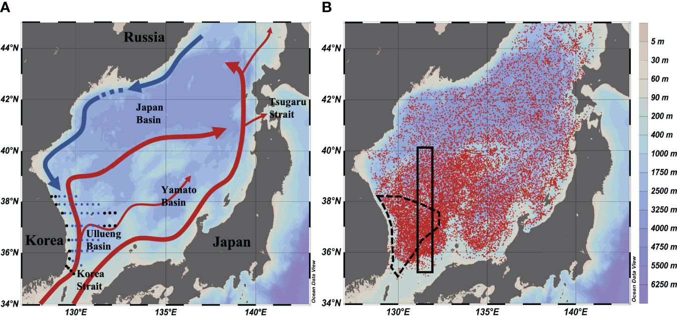
Figure 1 Map of the East Sea and stations for (A) National Institude of Fisheries Science (NIFS) hydrographic data and (B) Argo float (1999–2015). Red and blue arrows in panel (A) denote warm and cold surface currents. All NIFS station data are for thickness comparison with Argo data and the only blue stations are for studying long-term variability of the East Sea Intermediate Water (ESIW). The black solid-line rectangular box shows the area for which Argo data were taken for Figure 2. The area with dashed lines is for Figure 3.
2.1.2 Argo Float Data
Temperature and salinity profile data obtained from the Argo floats between 1999 and 2015 were used to compare the temperature-based and density-based ESIW thickness. The hydrographic data obtained from Argo floats were neither uniform in space and time, nor was their observation period long enough to observe long-term variability; however, they can be a good countermeasure to support the analysis of shipboard data. The 36 profiling floats in the ES were deployed by the University of Washington, USA, in 1999 for the Office of Naval Research program. The remaining floats were deployed annually by the Korea Institute of Ocean Science and Technology and the Korea Meteorological Administration & Korean National Institute of Meteorological Sciences as part of the Korean Argo program. In total, about 22,000 temperature and salinity profile data were produced from January 1999 to December 2015 from more than 150 floats (Figure 1B). Basically, all the float data were processed by following the delayed mode quality control procedure from the Argo data management team (Wong et al., 2019), but because the natural property variability in the ES is 10 times smaller than that in the open ocean, the data quality was improved by the method optimized for the ES, and the estimated one-standard salinity error was reported to be 0.004 g kg−1 (Park and Kim, 2007).
2.1.3 Satellite Altimetry Data
The satellite-derived sea surface height (SSH) data were also utilized to analyze whether spatial distribution and temporal variability of the ESIW thickness depend on the upper ocean circulation patterns. The spatial structures of the upper ocean circulation in the southern part of the ES are clearly shown in the SSH maps (Choi et al., 2004; Park and Nam, 2018). The SSH data are a merged product of multiple altimeter missions, daily gridded onto 0.25° × 0.25° over the time period January 1993 to December 2020 (https://resources.marine.copernicus.eu/). After removing the seasonal variability using the 1-year box-car filter method, the monthly mean SSH was obtained to compare SSH with the ESIW thickness and isotherm depths.
2.1.4 Arctic Oscillation Index
The daily AO Index was provided by the Climate Prediction Center, National Oceanic and Atmospheric Administration (NOAA), USA (https://www.cpc.ncep.noaa.gov/), which is constructed by projecting the daily 1,000 mb height anomalies poleward of 20°N onto the leading EOF mode. The time series are normalized by the standard deviation of the base period, 1979−2000. The leading Empirical Orthogonal Function (EOF) pattern of AO is obtained using the monthly mean height anomaly dataset.
The AO is a representative phenomenon that greatly affects the atmospheric environment, especially during winter in the ES. There have been several studies to show the correlation between the AO and the water mass properties of the ES and the great influence on the surface water temperature and wind patterns of the ES (Isobe and Beardsley, 2007; Cui and Senjyu, 2010; Nam et al., 2016). In addition, a positive winter AO strongly correlates with warmer winters over East Asia by enhancing the Polar westerly jet (c.f. Park et al., 2011; Wu et al., 2015). The AO Index has been filtered with box-car windows of 3 years, whose raw data are shown in Supplementary Figure S2.
2.2 Methods
2.2.1 Density-Based East Sea Intermediate Water Thickness
When a large amount of water mass volume is formed, the vertical layer of the corresponding water mass defined by the range of isopycnal surfaces must be thicker while looking at the area that is not far from the formation site, and the volume change of the water below and above it can be ignored. Even though the thickness of the water mass can be changed under the influence of mixing after being subducted, it is assumed that mixing-induced thickness change will not produce interannual-decadal variability. However, the ESIW thickness can change by not only the amount of formation but also the expansion and contraction of water volume above and below it; therefore, the analysis must be cautiously performed.
Usually, since water masses easily expand along isopycnal surfaces, vertical range occupied by the water masses is often defined by density ranges. Kim et al. (1999) exhibit that the ESIW has a density range between 26.9 and 27.3 σθ. In this study, the density-based ESIW thickness is defined as the depth difference of those two isopycnal surfaces suggested by Kim et al. (1999). However, as described above, the thickness of the ESIW based on density could not be accurately calculated because of the low quality of NIFS salinity data. Thus, the density-based ESIW thickness is computed only using Argo float data to compare with the temperature-based thickness obtained from the NIFS data.
2.2.2 Evaluation of the Temperature-Based East Sea Intermediate Water Thickness
Before the ESIW thickness is calculated based on temperature only, the existence of a potential correlation between thickness and density must be examined. The red dot in Figure 2A is a comparison of potential density-based (26.9−27.3 σθ) and potential temperature-based (1°C−5°C) thickness using Argo float data within the NIFS observation area shown in Figure 1B. There is a clear linear relationship with each other (R2 ~ 0.78), but the temperature-based thickness is statistically underestimated.
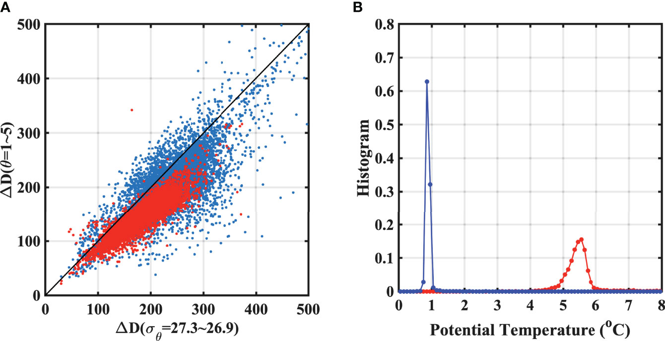
Figure 2 (A) Scatter plot between the density-based (26.9−27.3 σθ) and temperature-based (1°C −5°C) thickness obtained from Argo data. Red dots represent the data within the area denoted using dashed line in Figure 1B, and blue dots represent data from the whole East Sea. (B) Histograms of temperatures on the isopycnal surfaces of 26.9 and 27.3 σθ shown in red and blue lines, respectively, which are computed from the Argo data obtained from the area of dashed line in Figure 1B.
This is because the temperatures and densities at the ESIW top and bottom suggested by the previous studies do not match. Figure 2B shows the histograms of the temperatures on the isopycnals of 26.9 and 27.3 σθ. The temperature-based range of the ESIW (1°C−5°C) is found to be quite conservative compared to the density-based one. The temperature range corresponding to the density range may be 0.8°C−5.6°C in terms of median values. The width of the temperature histogram for 26.9 σθ is wider than 27.3 σθ. However, it is simply because of the difference in vertical gradient of temperature. In fact, the mismatch of the ESIW bottom boundary based on temperature and density is mainly responsible for the underestimation of the temperature-based thickness. Unfortunately, the temperature at the ESIW bottom cannot be set to 0.8°C instead of 1.0°C because the ESIW bottom is often deeper than 500 m, which is the maximum NIFS observation depth.
Figure 3 shows the density- and temperature-based ESIW thicknesses calculated from Argo float data within the NIFS observation area in time series. The 5-month moving averaged lines demonstrate that the temperature-based thickness (green) is underestimated by about 30% compared to the density-based thickness (black). However, in terms of variabilities, they fluctuate almost identically with the high correlation of 0.97. The green dotted line, which represents 1.3 times the temperature-based thickness, is comparable to the density-based one, confirming that the temperature-based thickness can be used as a substitute variable indicative of the thickness variability of the ESIW.
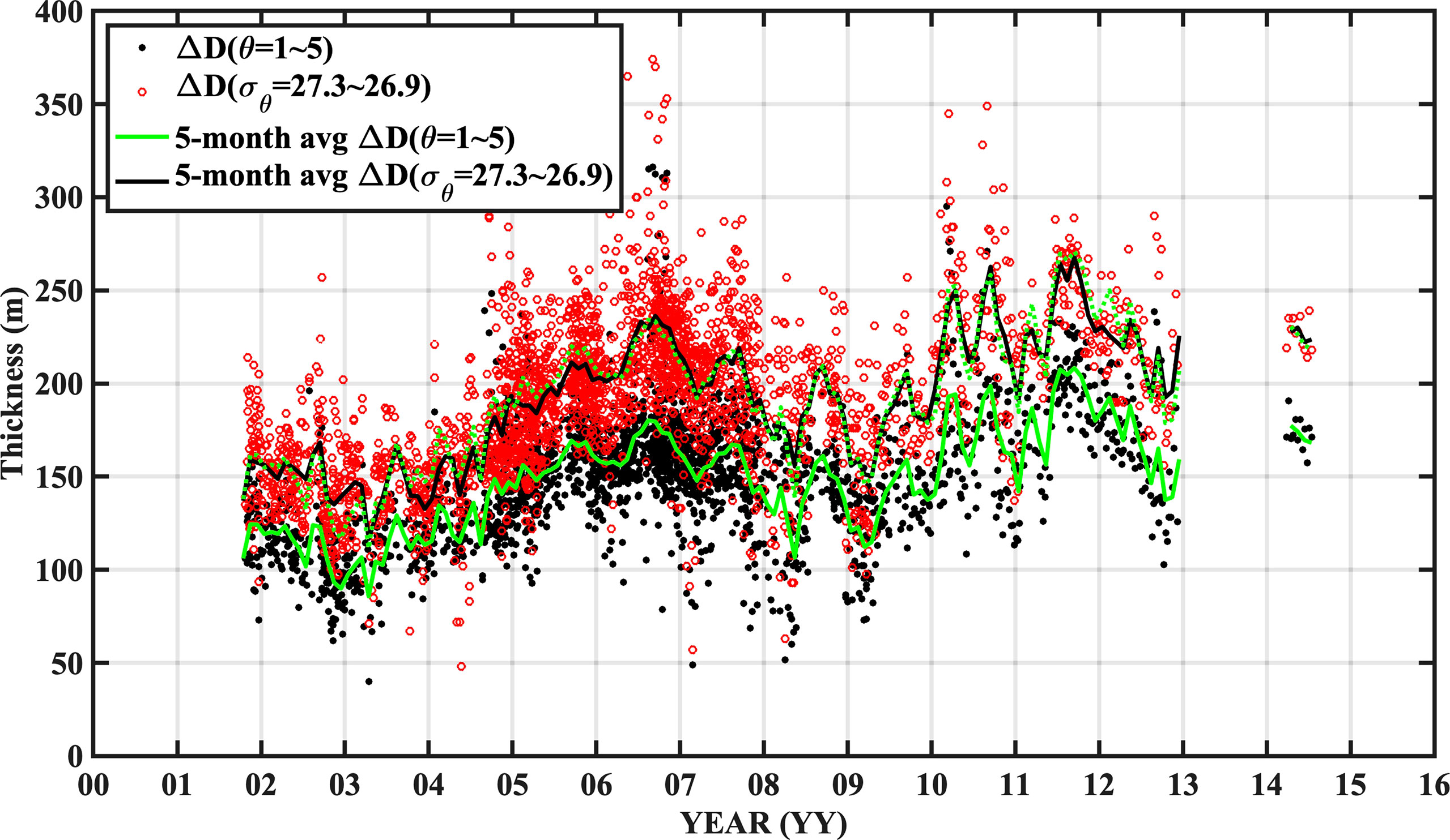
Figure 3 Time series of temperature-based thickness and density-based thickness in the area denoted by the dashed line (Figure 1B). Black and open red dots denote temperature- and density-based thickness, respectively. Green and black lines show the 5-month moving averages of the temperature-based and density-based thickness, respectively. The green dotted line represents 1.3 times the temperature-based thickness.
The ESIW thickness was first calculated from the NIFS profile data, and stations that were not in the temperature range of 1°C−5°C were excluded from the calculation. From 1978 to 1981, the northernmost Line 107 (38.21°N) observation was not made at a depth of 500 m, so it was not counted. The NIFS shipboard measurements are usually scheduled to be carried out in February, April, June, August, October, and December every year, but the observations were not conducted on the same day every year due to weather conditions. Therefore, due to missing data or temporal irregularities, a linear interpolation was performed at intervals of 2 months and 0.1° for spatial analysis, and seasonal variations were eliminated by applying a 14-month box-car filter.
2.2.3 Mean Temperature Reconstruction by Basin-Wide Average of Isothermal Layer Depth
To analyze and understand temporal variability of the ESIW thickness and to examine how the vertical structure of basin-wide averaged temperature changes with time, a basin-wide average of temperature profiles was performed in terms of isothermal layer depth rather than a simple depth coordinate. The horizontal circulation structure of the observation area and the presence of mesoscale eddies play an important role in determining the thermocline depth. In such an environment, when basin-wide averaged temperature was calculated on pressure or depth coordinates, fictitious vertical diffusion occurred, creating a vertically smoothed temperature structure (Lozier et al., 1994; Nurser and Lee, 2004) and affecting the thickness in the thermocline water. Therefore, to prevent such an error, thicknesses of the isotherm layers by 0.5°C bins were spatially averaged and then vertically integrated to calculate the depth value of each temperature as follows.
where T denotes potential temperature; D, the isotherm depths; and A, the domain area. Ttop and Tbottom are 15°C and 1°C, respectively.
However, the basin-wide averaged temperature estimated in this manner has a limitation, especially near the surface and the bottom in that predetermined isotherm layers were not found. Therefore, it is suitable only for the middle or deep layers where the isotherm layers are mostly found. In this study, the problem is minimized because the observation area is far enough away from the formation area and mostly below the thermocline. In this calculation, Ttop was set to 15°C and the temperature of 9°C–15°C can outcrop in the limited area of the observation domain only in winter. In this case, the depth of the corresponding isotherm surface was taken as 0.
To estimate the basin-wide averaged temperature, the isotherm layers were obtained at 0.5°C intervals from all the NIFS temperature profile data, and seasonal variations were removed using 14-month moving averages. The filtered data were reconstructed in the form of an equal grid using three-dimensional (3D) linear interpolation to obtain a spatial grid of 0.1° × 0.1° and a time grid of 2 months. By averaging the gridded isothermal layer data over the observation area, the depth of each isothermal layer was calculated temporally and converted into temperature profiles.
3 Results
3.1 Variability of the East Sea Intermediate Water Thickness and Property Based on Argo Float Data
Considering the Argo float data obtained between 131°E and 132°E as cross-sectional data in a meridional direction (35.5°N−40.0°N), Figure 4A shows the variation in the layer thickness of isopycnal surfaces between 26.9 and 27.3 σθ where the ESIW resides, and Figure 4B presents the salinity variation on the 3°C isotherm surface. Because the Argo data have a spatiotemporal irregular distribution, it is interpolated by the Gaussian weighted average method with a temporal (1.5-year) and spatial (0.25°) decorrelation scale.
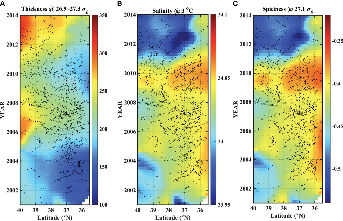
Figure 4 (A) Hovmoller diagram for the ESIW thickness (meter) from Argo float data within the solid-line rectangular box (35°N−40°N, 131°E−132°E) in Figure 1B. (B) The same as panel (A) but for salinity (g/kg) at 3°C and (C) for spiciness at 27.1 σθ. Black dots denote where the Argo data are.
The thickness is higher in the north close to the formation site and becomes thinner further south (the potential vorticity is not conserved). In terms of temporal variability, the layer is thick in 2005−2008 and in 2011−2014, and it expands to the south over time. The rate of expansion could not be accurately determined because of the greatly smoothed sparse data, but it appears to take about 0.5 to 1.5 years at latitudes 40°N to 38°N. Importantly, the spatiotemporal variation of thickness is quite similar to the pattern of the salinity on the 3°C isotherm surface that corresponds to the central part of the ESIW. Relatively low-salinity properties appear in the years of large thickness, and high-salinity properties appear when the thickness is thin. However, the temporal variability of salinity does not have a linear relationship with the thickness (not sensitive on isotherm surfaces). For example, at latitude 39°N, even though there is no significant difference in thickness between 2007 and 2013, there is a noticeable difference in salinity.
A similar trend was observed for spiciness on the isopycnal surface of 27.1 σθ. Spiciness shows whether a water mass is spicy (warmer and saltier) or minty (colder and fresher) in a specific density aspect, which is the orthogonal quantity to isopycnals on the θ-S diagram (McDougall and Krzysik, 2015). Because the ESIW density is predominantly controlled by water temperature, there is little difference in the spatiotemporal structure of spiciness on the isopycnal surface or salinity on the corresponding isothermal surface (refer to Supplementary Figure S3 for thickness of 1°C–5°C and salinity at 27.1 σθ). Although the salinity in 2011–2014 was 0.05–0.06 g kg−1 lower than that in 2005–2008, the effect of this salinity change on density is approximately 0.04 kg m−3, which is one-tenth smaller than the total density range of the ESIW (0.4 kg m−3).
Therefore, the thickness variability close to the formation site is strongly linked with that in the southern area. As Park and Lim (2018) pointed out, the ESIW salinity is influenced by the characteristics of the fresher surface water advected into the formation site. However, the amount of fresher surface water entering the formation site does alter the ESIW salinity yet does not significantly affect the amount of formation because its effect on density is small.
3.2 Long-Term Variability of the East Sea Intermediate Water Thickness
Figure 5 presents the temperature-based ESIW thickness variability (hereafter referred to as the ESIW thickness) for which the seasonal variability is removed at each station (Raw data can be found in Supplementary Figure S4). The color indicates the latitude of each NIFS measurement station, as shown in Figure 1. Interannual-interdecadal variability clearly exists, and the variabilities tend to appear similarly over entire stations. Compared with the ESIW thickness fluctuations obtained from the Argo float data in 2002−2013 (Figures 2, 4), the patterns of thickness variability are comparable between Argo and NIFS data; for example, the larger thickness observed in the years 2005−2008 and 2010−2013.
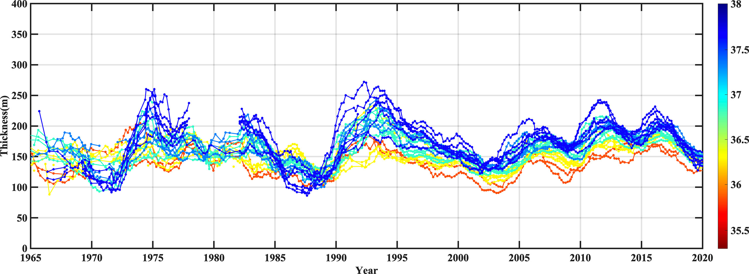
Figure 5 Fourteen-month moving averaged time series of the ESIW temperature-based thickness obtained from the NIFS data (1965−2020). Each color denotes latitudes of the corresponding NIFS stations. Raw data are shown in Supplementary Figure S4..
Figure 6 shows the spatial distribution and principal component (PC) time series of the first and second EOF modes of the ESIW thickness, respectively. The first mode accounts for 75.7% of the total variance, and the second mode accounts for only 6.4%. Most of the ESIW thickness variations can be explained in the first mode. The spatial distribution of the EOF first mode has positive values over the observation area, so it fluctuates stronger in the north and weaker in the south according to the pattern shown in the PC first spatial mode. The first mode PC time series sufficiently captures the temporal fluctuations shown in Figure 5. The periodic fluctuations of 3–6 years and long-term fluctuations of 15–18 years were predominant, rather than the year-to-year variations suggested by Kim et al. (1999). It is noted that the fluctuation pattern before the 2000s tended to increase rapidly and then decrease slowly in interdecadal timescales, while the fluctuation pattern seems to have changed in the 2000s and 2010s, although there is the limitation of observation period.
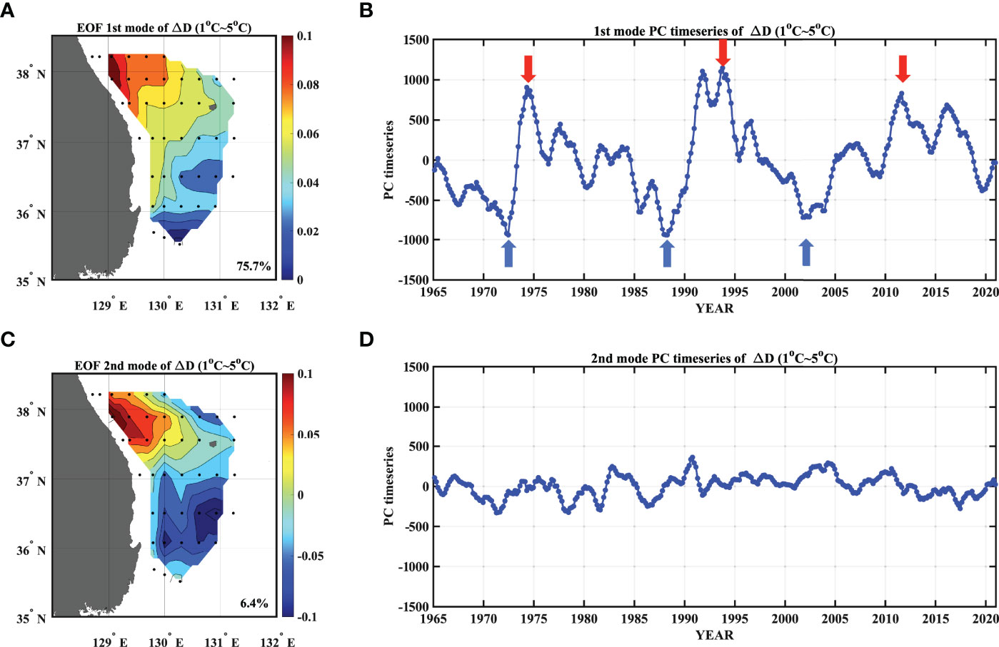
Figure 6 (A) EOF first mode loading vector for the ESIW thickness, (B) EOF first mode PC time series for the ESIW thickness, (C) EOF second mode loading vector, and (D) EOF second mode PC time series.
From the spatial distribution of the ESIW thickness when the negative and positive peaks appear in the PC time series, it can be confirmed that the thickness varies over the entire domain (Figure 7). The northwestern part of the domain is thicker and the southeastern part is relatively thin in the years with positive peaks (1974, 1993, and 2011). The spatial structure of the EOF first mode sufficiently captures the characteristics of the observation data.
The temporal change of spatial pattern of the thickness is not likely affected by the upper ocean circulation patterns (Figures 8A). The East Korea Warm Current and the Ulleung Warm Eddy are dominant features that control the surface circulation in the southwestern part of the ES, manifested in the spatial map of SSH that mostly represents the first baroclinic structure (Choi et al., 2004; Park and Nam, 2018 ). The SSH map shows that the East Korea Warm Current moves northward along the east coast, and then separates from the coast at a latitude of 37°N–38°N and flows southward at around 131°E. These features vary over the years. Additionally, the warm eddy structures with locations and strengths differently over the years. However, those upper circulation structures do not appear in the ESIW thickness shown in Figures 7D–F.
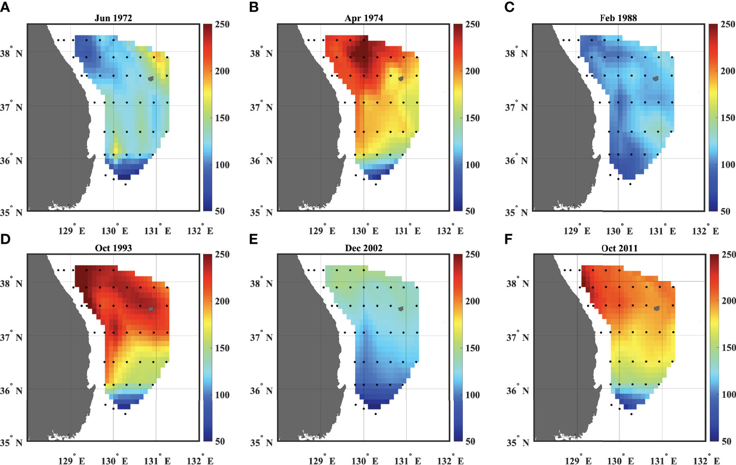
Figure 7 Spatial distribution of the ESIW thickness at the peak years of the EOF first mode PC time series shown in Figure 6B such as (A) June 1972, (B) April 1974, (C) February 1988, (D) October 1933, (E) December 2002, and (F) October 2011.
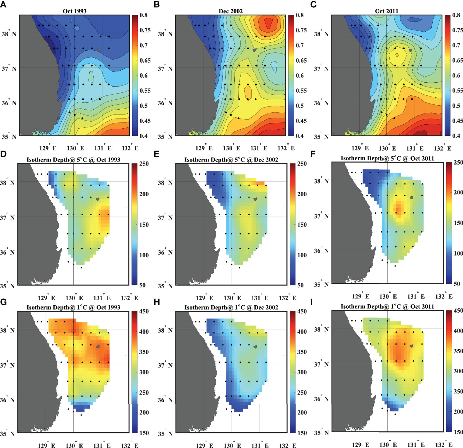
Figure 8 Spatial distribution of monthly mean sea surface height in (A) October 1993, (B) December 2002, and (C) October 2011 where the ESIW thickness peak and nadir are shown in Figures 7D–F. Spatial distribution of isotherm depth of (D–F) 5°C and (G–I) 1°C over the same months as panels (A–C).
Alternatively, the isotherm depth spatial structures of 1°C and 5°C are clearly influenced by the upper circulation structure. We interpret that the upper ocean circulation pattern produces shoaling and deepening of the isotherm surface but does not significantly affect the isothermal layer thickness corresponding to the ESIW. It can be also confirmed with Argo data that the spatiotemporal distribution of the ESIW thickness is not directly related to the local upper circulation pattern (Supplementary Figure S5).
We demonstrated that the first mode temporal variability of the ESIW thickness mostly has basin-wide fluctuations rather than mesoscale structures. Therefore, to investigate the variability of the vertical structure of temperature associated with the ESIW thickness variability, the basin-averaged temperature will be examined in the next section.
3.3 Basin-Wide Averaged Temperature
Figures 9A, B show the basin-averaged temperature on z-coordinate and isotherm layer averaged temperature, respectively. Due to the fictitious diffusion, the thicknesses of the isotherm layers in the thermocline are thicker overall in Figure 9A than those in Figure 9B. In particular, the structure of the thermocline is greatly smoothed out, for example, resulting in the thickness of 1°C–5°C in Figure 9A being thicker by 25% or more. Also, the interannual variabilities of the isotherms of 1°C and 2°C have unrealistically large amplitudes in the z-coordinate averages. This is more likely a result of contamination by spatial variability of isotherms rather than the actual basin-wide temporal variability. Thus, in this study, Figure 9B was used to see the basin-averaged temperature structure to understand the ESIW thickness fluctuations.
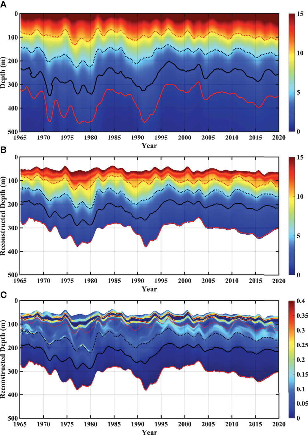
Figure 9 (A) Temporal variability of mean temperature profile averaged over the NIFS observation domain on the depth (z) surfaces. (B) Same as panel (A), but on the isothermal surfaces. (C) Vertical temperature gradient of mean temperature profiles shown in panel (B) Unit of panel (C) is °C/m. Red lines, black lines, black dotted lines, and red dotted lines denote 1°C, 2°C, 5°C, and 10°C isotherms, respectively.
The ESIW corresponds to the area between the red line and the black dotted line in Figure 9B. The decadal variability of the 1°C isotherm appears to correlate with isotherms of higher temperatures in the upper layer, especially before the mid-1990s. Furthermore, the dominant decadal-scale variabilities with relatively large amplitudes below 5°C decreased after the mid-1990s and the interannual scale variabilities are more pronounced. However, because isotherms with temperatures higher than 10°C show no predominance on decadal-scale variability before or after the mid-1990s, the decadal scale variability possibly originates from the deeper ocean.
One striking feature is that the thickness between 5°C and 10°C isotherms has remarkably decreased since the mid-1990s. Figure 9C is the vertical temperature gradient estimated from Figure 9B and demonstrates that the temperature gradient in the thermocline layer has significantly increased since 1995. This increase occurs because the isotherm depth at 10°C does not change significantly around 100 m, yet the isotherm depth at 5°C becomes shallow. As shown in Figure 10A, the linear trends of the 2°C and 5°C isotherm depths are −5.9 ± 1.7 m/10 years and −2.3 ± 1.4 m/10 years, showing a strong shallowing trend within 95% confidence level. Alternatively, the 1°C isotherm depth did not show a significant trend at +1.0 ± 2.0 m/10 years, while the 15°C isotherm depth showed a clear deepening trend at +2.4 ± 0.5 m/10 years, implying the warming trend. The deepening trend of the upper isotherms weakens as it goes deeper, and the trend sign changes around the 8°C isotherm. The clear shallowing trends below 10°C are responsible for the decrease of the thickness between 5°C and 10°C isotherms. It is noted that, in the z-coordinate averages, the trends of the isotherm depths are difficult to be identified and also the increase of vertical temperature gradient in the upper thermocline is not clearly seen (not shown).
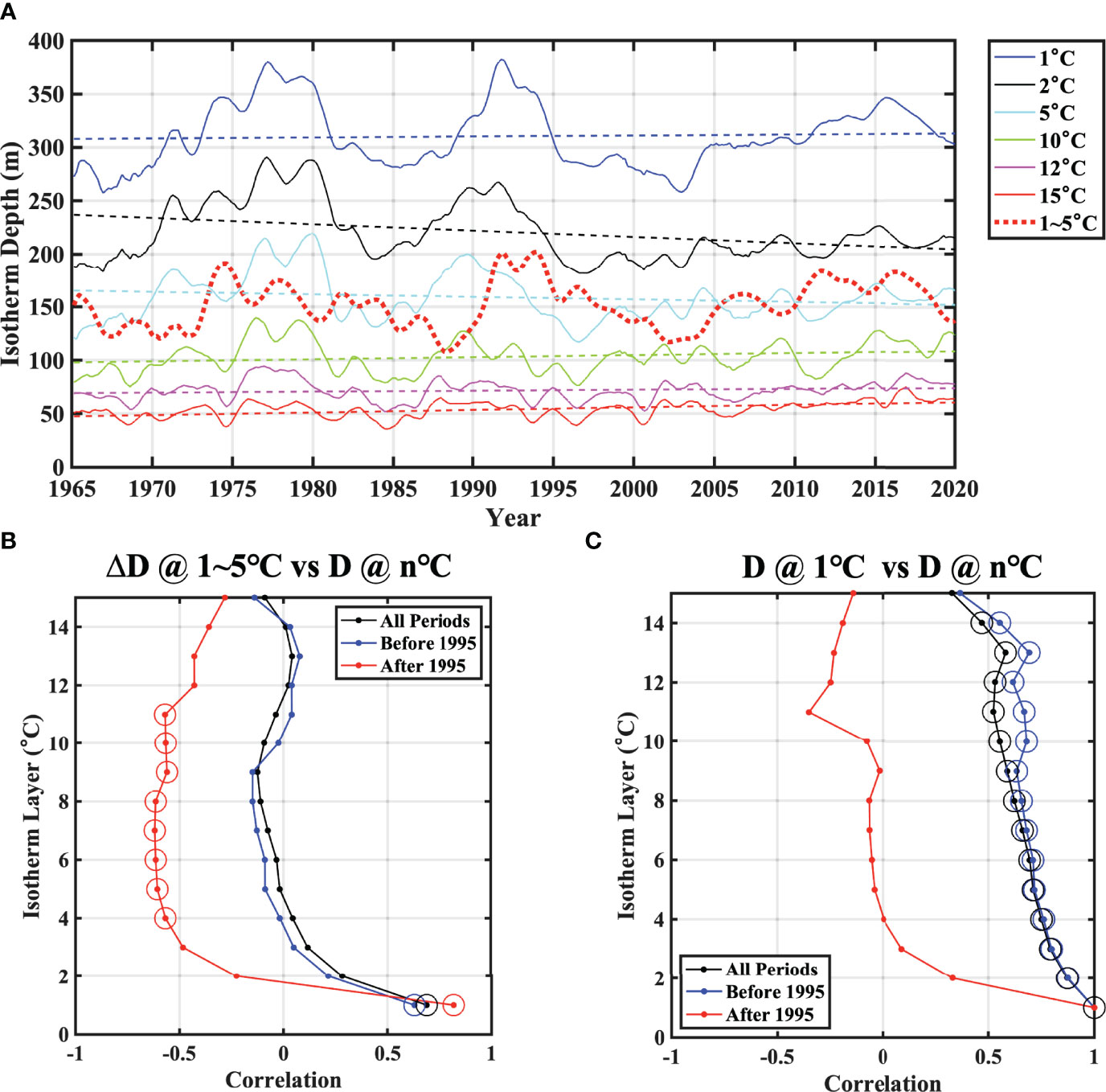
Figure 10 (A) Temporal variability of isotherm depths of 1°C, 2°C, 5°C, 10°C, 12°C, and 15°C and the ESIW thickness computed from the mean temperature profile data shown in Figure 8B. Dotted lines are linear fits of each isotherm depth. (B) Correlation between the ESIW thickness shown in panel (A) and other isotherms (in °C). (C) Correlation between the isotherm depth of 1°C and other isotherms. In panels (B, C), black line is by using the data for the whole time period. Blue line is from 1965 to 1994 (30 years), and red line is from 1995 to 2020 (25 years). Open circles denote where the significances are above 95%.
To analyze the relationship between the ESIW thickness and isotherm depths, the thickness of the isotherms between 1°C and 5°C in Figure 9B is shown as a red dotted line in Figure 10A. The variability of the thickness computed from the basin-averaged temperature (Figure 10A) is comparable to the first mode PC time series in Figure 6B. The correlations between the variation of the ESIW thickness and the corresponding isotherm are presented in Figure 10B. With the data before the year 1995, the ESIW thickness has a significant positive correlation only with the 1°C isotherm, but after 1995, it has negative correlations with the isotherms between 4°C and 11°C, implying that when the ESIW thickness is thick, those isotherms appear shoaling.
The correlations between the 1°C isotherm and other isotherms have significant positive correlations before 1995, but after 1995, the correlation almost disappears, as shown in Figure 10C. It should be noted that any linear trend was removed for estimating each correlation. Before 1995, the 1°C isotherm variability dominates that of the other upper isotherms in the thermocline layer. However, after 1995, the 1°C isotherm does not vary with the upper isotherms anymore.
Based on the above results, one scenario can be considered within the framework of the 1D advection–diffusion model of Munk (1966) in terms of the thermocline formation and maintenance. If the thickness variation of the ESIW before the mid-1990s is predominantly determined by the change in upwelling of the deep water below the intermediate water in the ES, it should be primarily expressed as a variability at the 1°C isotherm depth, and this effect would also be projected onto the upper isotherms. Because there is vertical diffusion that is stronger in the upper thermocline layer with a higher vertical temperature gradient, and the upper ocean temperature is constrained by the atmospheric condition and oceanic inflow, the effect of deep-water upwelling should be weakened while going up. In that case, the correlation between the ESIW thickness of 1°C–5°C and the isotherm depth of 1°C can be positive. Conversely, if the upwelling effect of the deep layer was significantly decreased since the mid-1990s, the ESIW variability itself must primarily control the upper isotherm variabilities, producing shoaling of 5°C isotherm as the ESIW layer thickens. Therefore, this process could explain the results showing a positive correlation between the ESIW thickness and 1°C isotherm and a negative correlation with 5°C isotherm.
3.4 Spatial Basin-Wide Averaged Temperature
If the temporal variabilities of isotherms in the thermocline were mainly due to upwelling of the deep layer before the mid-1990s and the volume change of the ESIW itself after the mid-1990s, there should be some difference manifested in the spatial distribution of the ESIW thickness for the two periods. Firstly, the spatial correlation maps of the ESIW thickness with time lags are presented in Figure 11. Figures 11A, B show the maximum correlations of the ESIW thickness at 37.5°N and 130.5°E (shown in blue diamonds) as a reference point and in the rest of the observation area. Figures 11C, D show the time lags where the maximum correlation coefficients appear. Except for south of 36°N, the results are not sensitive to the point of reference.
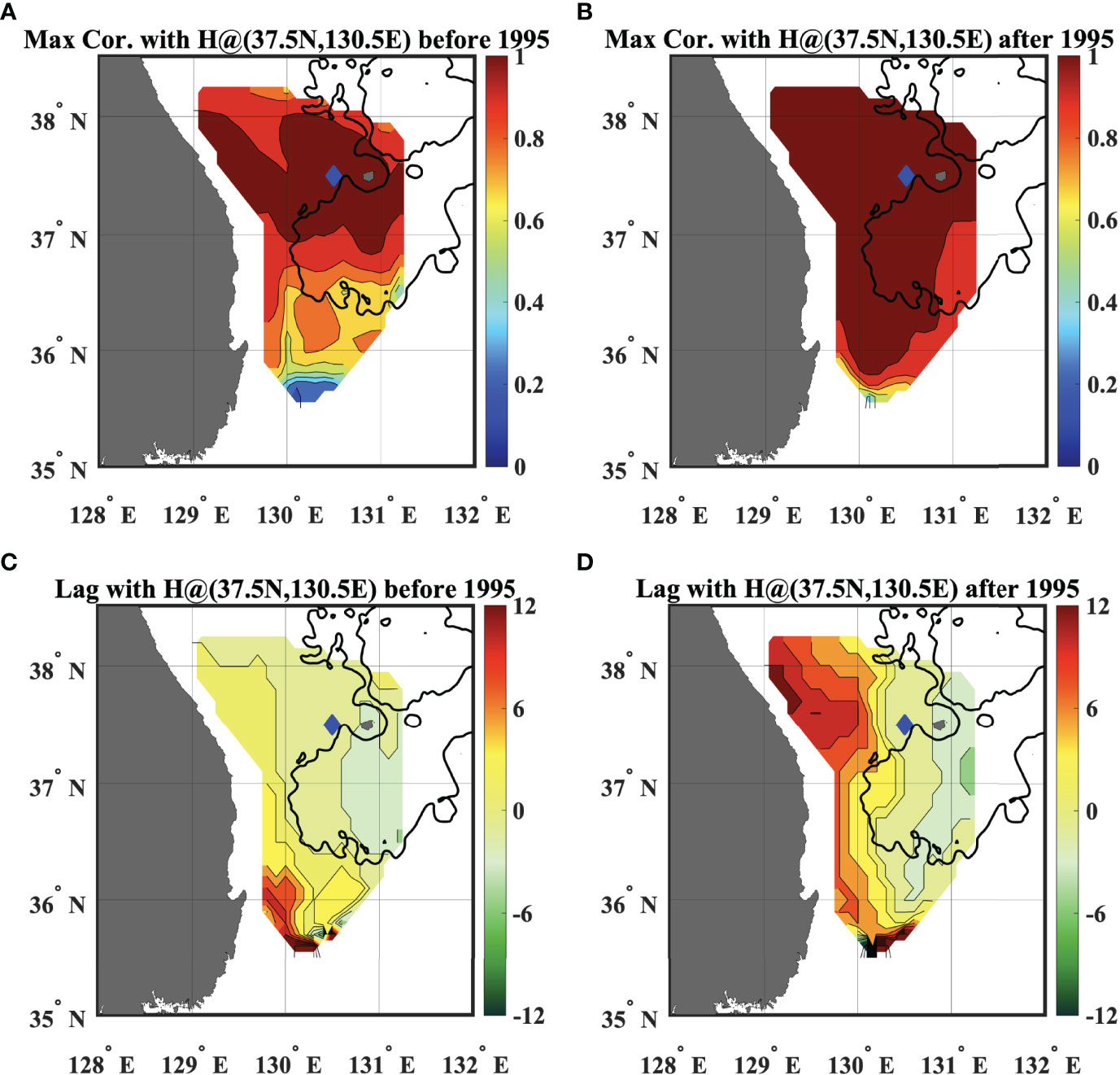
Figure 11 Spatial maximum correlation map of the ESIW thickness with the reference point at 37.5°N 130.5°E (A) from 1965 to 1994 and (B) from 1995 to 2020. Panels (C, D) show the monthly lag where the maximum correlations in (A, B) are, respectively. Blue diamonds denote the reference point. Contour intervals are 0.1 in (A, B) and 2 months in (C, D).
The maximum correlation has a high positive correlation of 0.6 or more in most regions, except for the southern edge before and after 1995. This is consistent with the basin-wide feature of the interannual-interdecadal variability of the ESIW thickness in Figure 6. Interestingly, most regions, except for the southern waters, have time lags of less than 3 months before 1995 (Figure 11C), but a spatially distinct lag difference appears after 1995 (Figure 11D), although the ESIW thickness appears to be basin wide. From Figure 11D, these lags appear more clearly in the zonal direction than in the meridional direction, and the zonal difference of the lags is approximately 12–14 months. A positive lag implies that the thickness variability in the corresponding area leads that at the reference location. The results indicate that the ESIW thickness change emerges quicker along the continental shelf slope, followed by the change in the offshore area or the Ullueng Basin approximately a year later.
Figure 12 presents the meridional and zonal sections of the ESIW thickness based on 37.5°N and 130.5°E. As for the temporal variability of the meridional distribution, the thickness tends to be higher in the north and lower toward the south. However, as shown in Figure 11, the time lag of the variability between 38°N and 36°N is indistinguishably small in the bimonthly dataset. These characteristics, at least for the south of 38°N, are not significantly different from the Argo float data in Figure 2 (direct comparisons in Supplementary Figure S6Aand S6C). Notably, the thickness is larger in the north than the south where it is thicker, but the tendency is not always applicable when it is thinner. After 1995, such a meridional tendency still holds even with the thinner ESIW, but it was not clear before 1995. The temporal change of the zonal section (Figure 12B) remarkably demonstrates the phase difference of the thickness fluctuations in the western and eastern areas, especially after the mid-1990s, while hardly any zonal phase change appears before the mid-1990s. Such leading appearance of the thickness in the coastal area is also evident in the Argo float data (Supplementary Figure S6F, also see the comparable figure from the NIFS data shown in Supplementary Figure S6F). The solid line and dotted line in Figure 12B are the lines connecting crests and troughs in the ESIW thickness variability at 129.4°E and 131.2°E, respectively. The phase difference ranges from 10 to 14 months, which is comparable to the lag correlation, converting into the slopes of 14−20 km/month (0.4−0.6 cm s−1). In spite of the zonal lags, the thickness variabilities in the western and eastern sides are clearly correlated, at least after the mid-1990s. One might think that the ESIW signal in the offshore could be the one expanded from the coast (c.f. Shin et al., 1998). However, the amplitude of the thickness variability increased in both the western and eastern edges of the observation domain, as was clearly observed in Figure 12B from 2005 to 2015. If the ESIW thickness signal solely comes from the coast, its variability would simply become smaller as it goes to the offshore along the solid and broken lines in Figure 12B. Yet, as it goes from 130.5°E to 131.2°E, the peak thicknesses increase (decrease) along the solid lines (the broken lines). This behavior implies that the ESIW thickness in the eastern area does not depend solely on the thickness of the coastal area, despite the offshore signal being followed by the coastal one. Note that the thickness trough in the coastal region becomes thicker as it goes offshore and then becomes thinner as it reaches 131°E.
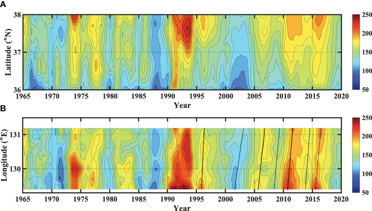
Figure 12 Spatiotemporal variability of the ESIW thickness on (A) latitude-time domain at 130.5°E and (B) longitude-time domain at 37.5°N. Black solid lines connect crests in the ESIW thickness at 129.4°E and 131.2°E. Black dotted lines are the same as the solid line but for troughs
The physical reason of the two-mode structure of the ESIW often found in the zonal hydrographic section (Cho and Kim, 1994) can be explained by the temporal variability of zonal structure of the ESIW thickness. If the NKCW and the ESIW were completely different water masses and were formed under different conditions or processes, their thicknesses should have no or low correlation between the coastal and offshore areas. However, according to the results of this study, the ESIW thickness variabilities near the coast and offshore are linked to each other with a year lag, implying that they are the same water mass but have different arrival times. Only with a snapshot observation data obtained at a specific time would it appear to be different water masses due to this time lag. Furthermore, as shown in Figure 4, the spatiotemporal variability of the ESIW thickness is closely related to that of its salinity property (also see Supplementary Figure S6). Therefore, the results shown in this study indicate that the two-mode structure of the ESIW shown in zonal hydrographic sections should result from the difference of the ESIW propagation path between near the coast and offshore, as previous researchers have suggested (Cho and Kim, 1994; Kim et al., 2006; Shin et al., 2007). It is important to note that even though the two-mode feature in the ESIW property was observed in the early 1980s, the zonal phase difference in the ESIW thickness was clearly visible only after the mid-1990s.
3.5 Correlation With the Arctic Oscillation Index
The AO Index and the ESIW thickness time series (Figure 13A) were observed to fluctuate together with a phase shift of a few years, especially before the 1990s. Therefore, the AO Index delayed by 2 years is redrawn in Figure 13B. Before the mid-1990s, the 2-year shifted AO Index and the ESIW thickness time series appear almost in phase; interestingly, they appear out of phase thereafter. The lag correlations between the AO Index and the ESIW thickness demonstrate a clear positive correlation of 0.8, with a lag of about 2.5 years before 1995 and a statistically significant negative correlation of 0.6 with a lag of about 1.5 years after 1995 (Figure 13C). This result shows that there has been a major change in the relationship with the AO Index since the mid-1990s.
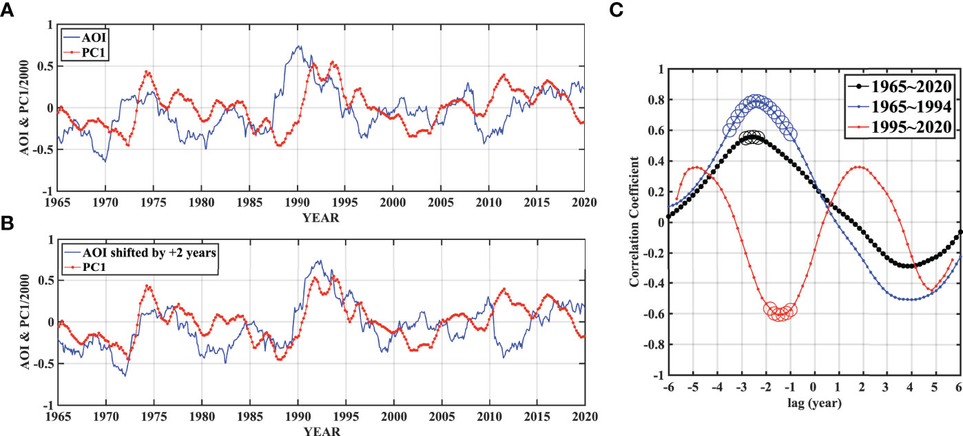
Figure 13 (A) Time series of 3-year moving-averaged AOI (blue) and the EOF first mode PC of the ESIW thickness scaled by 1/2,000 (red). (B) Same as panel (A) but AOI shifted by 2 years and (C) lagged-correlation diagram between AOI and first mode PC of the ESIW thickness. The black line is from the whole data. The blue line is from the data of 1965−1994 and the red one is of 1995−2020. The open circles denote where the correlations are above 95% significance levels.
The spatial correlation between the AO and the ESIW thickness also exhibits consistent features from the above results. Figure 14 shows the maximum absolute correlation and lag between the AO and the ESIW thickness before and after 1995 (Figures 14A, B) and the corresponding time lag (Figures 14C, D). Positive correlations with AO are dominant over the domain before 1995, while negative correlations prevail in a basin-wide manner after 1995.
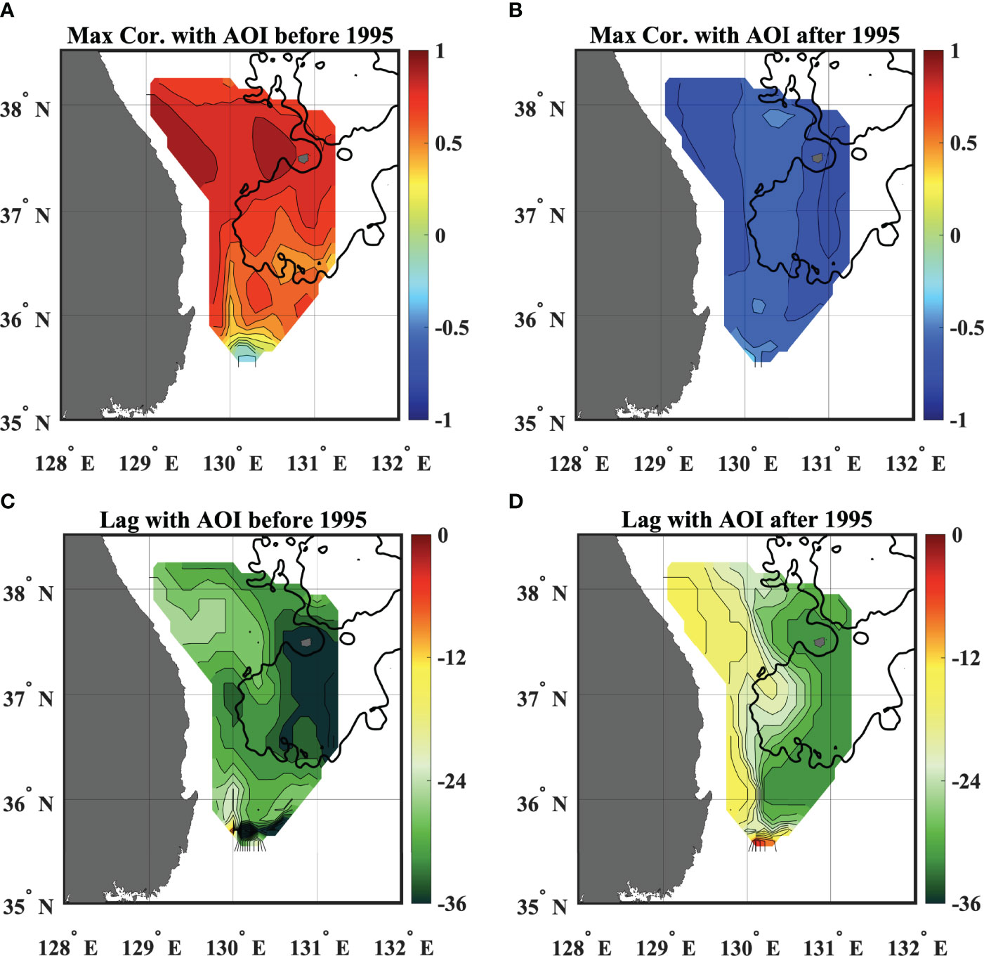
Figure 14 Spatial maximum correlation map of the ESIW thickness with AOI (A) from 1965 to 1994 and (B) from 1995 to 2020. (C, D) Are showing the monthly lag where the maximum correlations in (A, B) are, respectively. Contour intervals are 0.1 in (A, B) and 2 months in (C, D).
The lag time where the maximum absolute correlation appears is important. The overall lags before 1995 are larger than those after 1995 in the corresponding area. Before 1995, the AO fluctuations lead the ESIW thickness with a lag of larger than 20 months near the coastal region and a lag of about 28 months in the offshore area, the Ulleung Basin. However, after 1995, the ESIW thickness responded noticeably quicker to the AO in the vicinity of the ES coast with a lag of about 12 months and slowly in the Ulleung Basin with a lag of about 26 months. The zonal lag difference for the post-1995 period is much more pronounced than the pre-1995 period, reaching 14 months. In addition, these results are also consistent with the spatial correlation map of the ESIW thickness shown in Figure 11.
4 Discussion
To analyze the 55-year-long hydrographic data, the correlation was assumed to hold in the past as well. The main reason that the isotherm-based thickness has a strong correlation in time with the isopycnal-based one is that the effect of salinity on the ESIW density range in the southwestern ES is significantly smaller than that of temperature. In the hydrographic observation in 1969 (Senjyu, 1999), the salinity range of the ESIW salinity minimum layer in the southwestern ES was 34.00–34.02 g kg−1. Additionally, Kim and Chung (1984) showed a range of 34.00–34.05 g kg−1 from the observations in 1981, and Cho and Kim (1994) showed a range of 33.95–34.05 g kg−1 in the 1991 observations. All the salinity ranges of the ESIW in the past years are commonly found in the ESIWs of the 2000s. Therefore, it can be assumed that there was no dramatic salinity change in the past that could have affected the ESIW density.
It was also assumed that the error of temperature data after the quality control should be small enough, and that even if an error existed, it would not have spatiotemporal correlations. The first mode PC time series extracted through the EOF analysis and isothermal surface averaged ESIW thickness fluctuations appear almost similar, which could supposedly minimize the non-correlated error. Also, the spatial patterns of the thickness are consistent with the EOF and the basin-averaged analysis results. Thus, the long-term variability of the ESIW thickness in this study was confirmed to be robust.
The spatiotemporal variability of the ESIW thickness was also found to have a relationship with the ESIW salinity from the Argo data (2001−2014) in Figure 2 (also see Supplementary Figure S6). Based on the non-correlated features of the thickness with the local SSH or local wind stress curl (Supplementary Figure 5), and the thicker ESIW in the northern region close to the formation area, the variability information of the thickness seems relevant to the amount of formation volume, at least, for the Argo observation period. However, the ESIW salinity itself is not a strong factor in determining the formation rate because the salinity has little effect on the density range in the ESIW. Therefore, the ESIW salinity variability alone is not sufficient to explain the ESIW variation directly responding to climate variability. Indeed, as pointed out by Park and Lim (2018), it is consistent with the fact that the ESIW salinity is mainly determined by the amount of inflow of surface low-salinity water into the ESIW formation site by ocean advection rather than air-sea freshwater exchange.
The AO and the ESIW thickness since 1995 have almost the same lag along the ES coast as shown in Figure 14, whereas such alongshore tendency is not clear prior to 1995. The nearly uniform lag along the vicinity of the coast from 36°N to 38°N indicates that the advection or propagation timescale is shorter than 2 months of the hydrographic data intervals. Alternatively, the thickness signal travels along the coast faster than about 2 cm s-1. Also, if the same signal propagation process works for the northern area as the observation area, it can be inferred that it would not take as long as 12 months for the signal to propagate from the 40°N−41°N region where the ESIW is formed (Park and Lim, 2018) to the observation site. However, the time lag between the AO and ESIW thickness in Figure 14D is about 12 months. Similarly, the time lag of 26 months in the Ullueng Basin is too long to be considered as just the advection timescale of the offshore propagation path of the ESIW, suggested to be 6−12 months in previous studies (Yanagimoto and Taira, 2003; Yun et al., 2004; Park and Kim, 2013). Therefore, additional studies are required to explain the time lag between the AO and the water mass variability downstream.
More importantly, even though it has been confirmed that there is a persistent southward flow at the intermediate level along the eastern coast of the Korean Peninsula since the 1960s (Kim and Kim, 1983; Kim et al., 2006), the alongshore uniform lag is only prominent after 1995 and not before. This is a similar argument as the two-mode ESIW property addressed in the section Spatial Basin-Wide Averaged Temperature.
5 Conclusion
5.1 Long-Term Variability of the East Sea Intermediate Water Thickness
This study demonstrated that the long-term ESIW thickness variability has basin-wide features and clear interannual-interdecadal timescales, such as 15−18 years and 3−5 years as shown in the NIFS hydrographic data. The thickness variability increased toward the northern part of the observation area and decreased toward the south. This temporal thickness variation is not closely related to the SSH features, showing that the ESIW thickness variability is not dependent on the upper ocean circulation patterns.
The ESIW thickness variability is mostly determined by the 1°C isotherm fluctuation and is somewhat interacted with the upper layers above it. As for the horizonal structure, within the NIFS observation domain, the ESIW thickness fluctuates almost simultaneously in the meridional direction, while it has a clear zonal phase difference. However, the vertical and horizontal characteristics of the thickness variability are dramatically changed in the mid-1990s. The details are in the following section.
5.2 Regime Shift in the Mid-1990s
The following four distinct changes were observed concerning the long-term variability of the ESIW thickness beginning in the mid-1990s.
Changes in the vertical temperature structure of the upper ESIW layer: The vertical temperature gradient has been shown to increase, as the layer between 5°C and 10°C is significantly reduced since 1995. This appears to be because the 2°C−5°C isotherms are clearly shoaling, despite the deepening of the isotherms for 9°C and higher.
Changes in the correlation between the thermocline isotherms: There are nearly zero correlations between the ESIW thickness and the isotherms in the thermocline layer before 1995 with the exception of the 1°C isotherms but negative correlations with the 4°C−11°C isotherms after 1995. This implies that after 1995, as the ESIW becomes thicker, the upper layer is pushed up and shoaled. However, before 1995, all isotherms vibrated similarly with a slight phase difference, though with different amplitudes (smaller as it goes up). The ESIW thickness for this time period was mainly produced by the phase and amplitude difference between isotherms.
Changes in the spatial distribution of the ESIW thickness: Long-term variability of the ESIW thickness has time lags of several months depending on the locations. The fluctuations tend to occur first in the vicinity of the ES coast and appear later in the offshore, the Ulleung Basin. This zonal lag has become remarkable since 1995 and is related to the unique characteristics of the ESIW property suggested in a previous study where it appears as two modes in the zonal hydrographic section (Cho and Kim, 1994). Consistently, it has been reported that the ESIW flowing southward along the coast extends to the offshore to the Ullueng Basin in the zonal direction (Shin et al., 1998; Shin et al., 2007). Due to these lags, the ESIWs found near the coast and in the basin could be misinterpreted as different water masses because their properties look different from the hydrographic data obtained in a specific year.
Changes in the relationship with the AO representing atmospheric conditions associated with water mass formation: The AO and the ESIW thickness clearly have a positive and negative correlation before and after the mid-1990s, respectively. The lag with the AO is also different, where the lag is longer before the mid-1990s than after. Cui and Senjyu (2010) showed that the AO and Sea Surface Temperature (SST) at the formation site of Japan Sea Proper Water (JSPW) had out-of-phase fluctuations and also pointed out that the DO concentration at 1,000 m had a higher correlation with cold air outbreak (Isobe and Beardsley, 2007). Because the AO Index is closely related to the winter atmospheric condition in the ES, it is relevant to the water mass formation rate and is a type of volume flux. However, the DO concentration in the downstream area is a kind of reservoir property that is basically integrated by fluxes. Considering the advection timescale or ventilation timescale of the water mass, there should be still some lag between the formation rate (relevant to AO) and the reservoir characteristics (relevant to the thickness) depending on the variation timescale. Therefore, a further study will be conducted on why the AOI index and the ESIW thickness have such a high correlation with some time lags.
Based on the observational results, a working hypothesis is suggested to explain the changes of the ESIW thickness variabilities and the discrepancies from the previous studies discussed in the Discussion.
6 Suggestion of Working Hypothesis
6.1 Response of Intermediate Water on Changes of Meridional Overturning Circulation
Intermediate waters are generally found over the world’s oceans and located between the upper ocean water, which is strongly influenced by atmospheric conditions or upper circulation, and the deep water, which is formed in the limited cold region by atmospheric conditions in winter due to local convection or subduction in the MOC perspective. The MOC becomes closed as the deep water mixes with the upper ocean water, with the intermediate water acting as a conduit between the upper and deep water.
Assume that the deep ES consists of a single water mass like JSPW. From the perspective of the Stommel–Arons model (Stommel and Arons, 1960), JSPW will make nearly uniform upwellings as it fills the ES seabed, causing the isotherms to shoal, which will also shoal the ESIW layer. However, above the ESIW, because there is the TWW coming through the Korea Strait, the upper ocean in the southern part of the ES is continuously refreshed by the advected TWW. As a result, the ESIW will be eroded by the TWW in the upper ocean, and one can expect that the ESIW volume would decrease as the deep waters are expanded. Therefore, the ESIW thickness variation basically includes the amount of its own formation and the volume change of deep waters.
Because the ES is a marginal sea with a small area, atmospheric conditions in winter of a certain year will be simultaneously applied on various water masses with different formation processes. The deep-water formation area is known to be in the east of the NKF (Park et al., 2005) off the Peter the Great Bay, Russia, and the ESIW is formed in the west of the NKF (Park and Lim, 2018). The formation regions of the ESIW and deep water are close enough compared to the atmospheric mesoscale, so they seem to be under similar atmospheric conditions in wintertime when formed. Alternatively, if the winters in the ES were colder than normal, it would favor the formation of all water masses: intermediate, deep, or bottom waters. That might be a reason why the ESIW thickness is positively correlated with AO before 1995. This point will be discussed in the next section.
In the past, DO concentration in the deep sea of the ES has been reported to be rapidly decreasing (Gamo, 1999; Kim et al., 2001; Yoon et al., 2018). The DO concentrations at the water depth of 2,000–3,000 m decreased steadily from 1954 to 2015, and at 500–1,500 m, it increased briefly in the mid-1990s, then decreased again in the 2000s. As of 2015, the vertical DO structure below the intermediate layer is almost constant. If the formation of water mass below the intermediate was limited and became insensitive to AO conditions, the ESIW thickness would be inferred to vary purely with the amount of its formation.
6.2 A Possible Scenario of the East Sea Intermediate Water Thickness Change Under Global Warming
The following scenario is proposed to explain the distinct difference in characteristics related to the ESIW thickness variability in the southwestern part of the ES in the mid-1990s (Figure 15). Typically, the water mass formation rate should be determined according to the AO, and there is a time lag of 1–2 years until the effect appears in the observation domain.
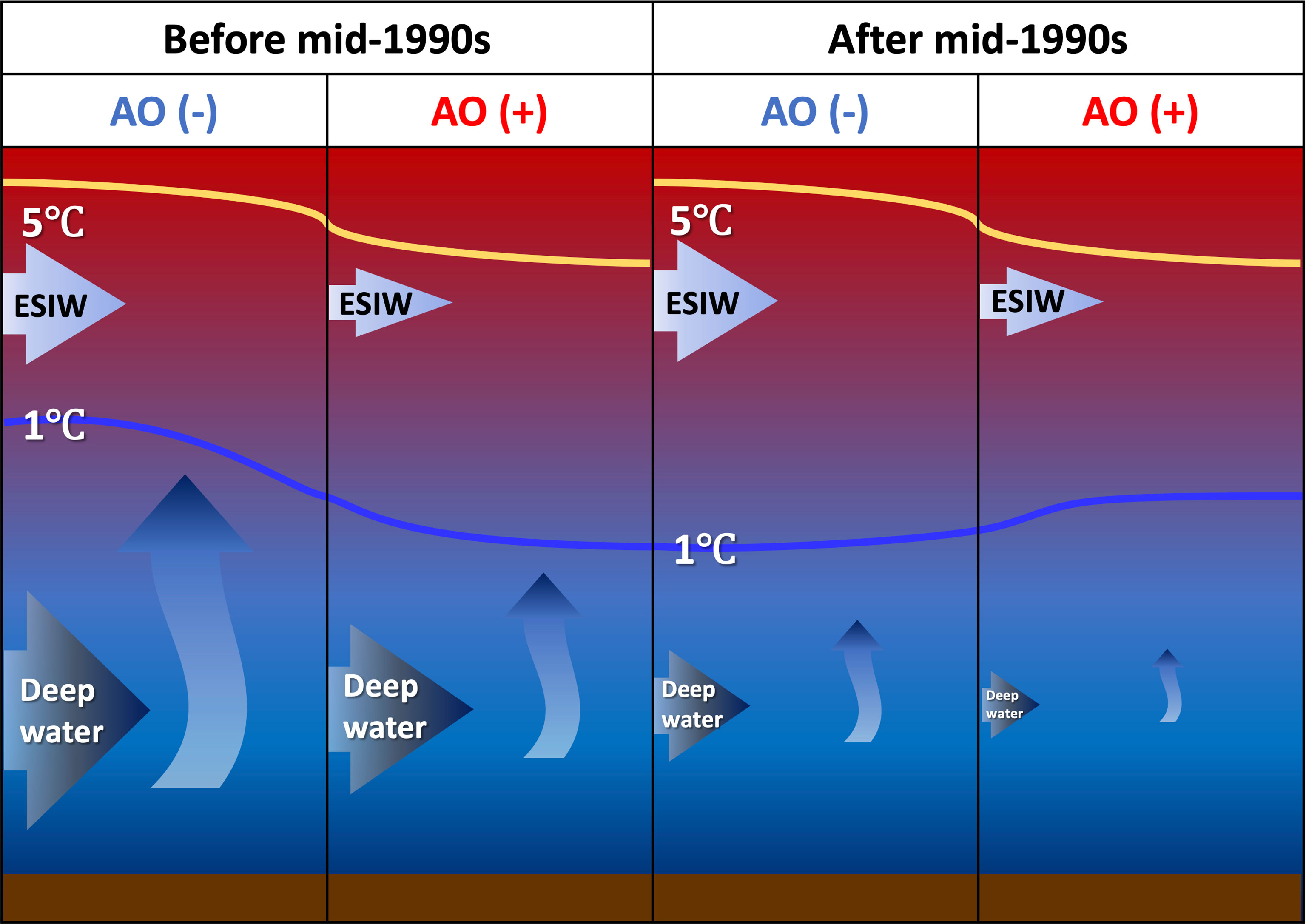
Figure 15 Schematic of the working hypothesis for the ESIW thickness change in the framework of the East Sea Meridional Overturning Circulation system.
As shown in Figure 15, before the mid-1990s, in the AO negative (positive) phase, cold (warm) winter conditions prevailed, and the formation of the ESIW and deep water (JSPW or CW+BW) was strengthened (weakened). Because the volume variability of deep water was much larger than that of the ESIW, it created shoaling (deepening) of overall isotherm surfaces under the thermocline in the southern seas of the ES. Therefore, the ESIW thickness variability can be primarily controlled by the change in the volume of deep water, and it shows in-phase behavior with AO.
However, since the mid-1990s, as the deep-water formation rapidly decreased under the influence of global warming and the AO-associated response was weakened, the overall isotherm surfaces were less affected by the volume change of the deep-water layer. As a result, the ESIW thickness was mainly determined by the ESIW formation itself, so it may be that the isotherm surfaces below and above the ESIW fluctuate in opposite directions.
The lag difference from the mid-1990s shown in the time series of the AO and the ESIW thickness in Figure 13 can also be interpreted consistently with the above scenario, such as the lag of 2.5 years before the mid-1990s and 1.5 years after. After the mid-1990s, the AO signal could be projected directly onto the much shallower and faster-circulating ESIW layer, resulting in the shorter lag, while before the mid-1990s, the ESIW thickness might respond more slowly to the AO because the signal came through the deep water.
Previously, several researchers have reported that the variability of deep-water properties (nitrate, DO, PO4, etc.) within the timescales of about 18 years exists in the ES (Watanabe et al., 2003; Cui and Senjyu, 2010), similar to the 15–18-year timescales shown in the ESIW thickness. Even though the deep-water properties and volumes may not have the variability with the same phase, the existence of such decadal variability in deep-water properties indicates that there should be also a variability in the volume of deep-water formation with a comparable timescale, producing the undulation of the upper isotherms.
The two-mode state of the ESIW salinity structure in the zonal conductivity-temperature-depth section is a distinct feature of ESIW that is not seen in other water masses. The zonal difference in the ESIW salinity has been reported in many previous studies since the 1980s (Kim et al., 1991; Cho and Kim, 1994). However, the zonal phase difference in the ESIW thickness has been shown only since the mid-1990s, which can also be explained by the above scenario. Because the ESIW thickness was mainly controlled by the deep-water volume change before the mid-1990s, such zonal phase difference of the thickness that could emerge due to deep-water layers is faded after the mid-1990s. In other words, the two-mode ESIW property existed before the regime shift appeared, but the fact that the two-mode thickness was seen since the mid-1990s proves that the thickness variation before the mid-1990s does not reflect the volume change of the ESIW itself.
7 Remaining Studies and Implications
To understand how the AO controls the water mass formation, accurate observational data at the formation site are required, but unfortunately, such data are not available. Satellite sea surface temperature data exist only since 1987, and reanalysis data are not suitable for such analysis because their resolution and accuracy are low in the ES. However, model-based studies can reveal a physical process to understand such a clear correlation between the ESIW thickness and AO in the future.
This study demonstrates that the sudden regime shift in the thermocline layer of the ES occurred in the mid-1990s. Clearly, a control process responsible for such rapid change must be understood. Additionally, the process should be reconciled with the ventilation timescale of the ESIW. The ventilation timescale, which is the time taken by the water mass to leave the formation site and arrive at the target area, might be about a few years or less based on the time-lag correlation between the AO and the ESIW thickness. However, the ESIW ventilation ages, estimated using chemical tracers like apparent oxygen utilization and partial pressure of chlorofluorocarbons, have varied over 10–23 years (Min and Warner, 2005; Kim et al., 2010). The large discrepancy in the ventilation timescale from the results in this study may be due to the strong vertical mixing of the ESIW with the TWW above it, which has low DO and chlorofluorocarbon concentration, because diapycnal mixing can greatly bias the chemical tracer-based age (Fine et al., 2017).
Modeling studies also estimated the ventilation time of the ESIW to be 6–10 years from the point of view of particle dispersion (Seung and Kim, 1997; Yoshikawa et al., 1999), and this may be related to the problem in which the low-resolution numerical models of the past underestimated the mean and eddy circulation at mid and deep layers (Park and Kim, 2013). The latest model results suggested that the ESIW arrived at the Ulleung Basin in a relatively short time of 1–2 years (Kim et al., 2021), which is comparable to the results of this study, although there is still a significant difference from the observed results in terms of the ESIW formation area. Because the ESIW ventilation timescale is important information, a study reconciling the chemical tracer-based, numerical model-based, and physical observation-based timescales is required.
Additionally, Yoshikawa et al. (1999) estimated the turnover time of the ESIW to be approximately 26 years by utilizing the ESIW formation rate and reservoir volume estimated by the numerical model. In perspectives of the long-term variability in the ESIW thickness shown in the NIFS data and the salinity variability shown in the Argo float data, the ESIW signal in the western part of the ES seems quickly refreshed within the order of years rather than lasting more than 20 years. Although it can propagate away to other basins in the ES, such as the Yamato Basin, the actual turnover time of the ESIW might be much faster than the previously simulated one. Indeed, Kim et al. (1999) showed that the ESIW property over the ES basins changed in a year-to-year manner, but additional research is required on this topic.
The scenarios discussed above explain the variation in the intermediate layer in terms of EMOC changes in response to AO under global warming. If the ES has been changing according to the scenario, the ESIW has the potential to serve as a good proxy for showing EMOC changes. Because the ES has a small domain size and ventilation timescales significantly shorter than that of the open ocean, the response to interannual-interdecadal atmospheric variability can appear quickly enough to be identified with the modern observations of less than 100 years. In addition, the ES is a unique marginal sea in that while the various water masses were formed under the influence of the same atmospheric conditions, they responded differently to global warming.
Although it is obvious that the water mass formation in winter is limited by global warming, it can be assumed easily that not all water mass formation rates are limited to the same extent. In the case of deep-water formation area in the ES, the mixed layer can be developed up to 1,000–2,000 m, which is favorable to the open ocean deep convection. However, because the vertical temperature gradient below the permanent thermocline in the ES is much smaller than the open ocean, even slight warming in the mixed layer can significantly reduce the mixing depth in winter, resulting in the slow formation rate. Alternatively, the ESIW is mainly formed above the thermocline by subduction due to the flow convergence in the mixed layer. Because the ESIW formation area is strongly stratified even in winter compared to the deep-water formation area, the mixed layer (Lim et al., 2012). depth could be less sensitive to a slight increase in surface temperature due to global warming.
Data Availability Statement
Argo float data were collected and made freely available by the International Argo Program and the National programs that contribute to it (http://www.Argo.ucsd.edu, http://Argo.jcommops.org). Satellite SSH data were processed by SSALTO/DUACS and distributed by AVISO+ (https://www.aviso.altimetry.fr) with support from CNES.
Author Contributions
JP conceptualized the study, performed all data analyses, and entirely contributed to writing the draft.
Funding
This research was a part of the project titled “Development of the core technology and establishment of the operation center for underwater gliders” funded by the Ministry of Oceans and Fisheries, Korea (1525012198). This work was also supported by the National Research Foundation of Korea (NRF) grant funded by the Korea government (MSIT) (NRF-2022R1A2C1004059).
Conflict of Interest
The author declares that the research was conducted in the absence of any commercial or financial relationships that could be construed as a potential conflict of interest.
Publisher’s Note
All claims expressed in this article are solely those of the authors and do not necessarily represent those of their affiliated organizations, or those of the publisher, the editors and the reviewers. Any product that may be evaluated in this article, or claim that may be made by its manufacturer, is not guaranteed or endorsed by the publisher.
Acknowledgments
I would like to thank my students, Bong-Joon Kim, In-Ha Seo, and Joo-Hee Park, who helped complete this article. In addition, I want to thank Dr. Y.-G. Kim, Prof. Y.-H. Kim, and Prof. S.-T. Yoon for their invaluable discussion on the earlier draft.
Supplementary Material
The Supplementary Material for this article can be found online at: https://www.frontiersin.org/articles/10.3389/fmars.2022.923093/full#supplementary-material
References
Choi B.-J., Haidvogel D. B., Cho Y.-K. (2004). Nonseasonal Sea Level Variations in the Japan/East Sea From Satellite Altimeter Data. J. Geophys. Res. 109, C12028. doi: 10.1029/2004JC002387
Cho Y.-K., Kim K. (1994). Two Modes of the Salinity-Minimum Layer Water in the Ulleung Basin. La Mer. 32, 271–278.
Cui Y., Senjyu T. (2010). Interdecadal Oscillations in the Japan Sea Proper Water Related to the Arctic Oscillation. J. Oceanogr. 66, 337–348. doi: 10.1007/s10872-010-0030-z
Fine R. A., Peacock S., Maltrud M. E., Bryan F. O. (2017). A New Look at Ocean Ventilation Time Scales and Their Uncertainties. J. Geophys. Res. Oceans 122, 3771–3798. doi: 10.1002/2016JC012529
Gamo T. (1999). Global Warming May Have Slowed Down the Deep Conveyor Belt of a Marginal Sea of the Northwestern Pacific: Japan Sea. Geophys. Res. Lett. 26, 3137–3140. doi: 10.1029/1999GL002341
Isobe A., Beardsley R. C. (2007). Atmosphere and Marginal-Sea Interaction Leading to an Interannual Variation in Cold-Air Outbreak Activity Over the Japan Sea. J. Clim. 20, 5707–5714. doi: 10.1175/2007JCLI1779.1
Kang D.-J., Kim J.-Y., Lee T., Kim K. R. (2004). Will the East/Japan Sea Become an Anoxic Sea in the Next Century? Mar. Chem. 91, 77–84. doi: 10.1016/j.marchem.2004.03.020
Kang S. K., Seung Y. H., Park J. J., Park J.-H., Lee J. H., Kim E. J., et al. (2016). Seasonal Variability in Mid-Depth Gyral Circulation Patterns in the Central East/Japan Sea as Revealed by Long-Term Argo Data. J. Phys. Oceanogr. 46, 937–946. doi: 10.1175/JPO-D-15-0157.1
Kim K., Chang K.-I., Kang D.-J., Kim Y. H., Lee J.-H. (2008). Review of Recent Findings on the Water Masses and Circulation in the East Sea (Sea of Japan). J. Oceanogr. 64, 721–735. doi: 10.1007/s10872-008-0061-x
Kim K., Chung J. Y. (1984). On the Salinity Minimum and Dissolved Oxygen Maximum Layer in the East Sea (Sea of Japan). Elsevier Oceanogr. Ser. 39, 55–65. doi: 10.1016/S0422-9894(08)70290-3
Kim C. H., Kim K. (1983). Characteristics and Origin of the Cold Water Mass Along in the East Coast of Korea. J. Oceanolog. Soc Kor 18, 73–83.
Kim Y.-G., Kim K. (1999). Intermediate Waters in the East/Japan Sea. J. Oceanogr. 55, 123–132. doi: 10.1023/A:1007877610531
Kim K., Kim Y.-G., Cho Y.-K., Takematsu M., Volkov Y. (1999). Basin-To-Basin and Year-to-Year Variation of Temperature and Salinity Characteristics in the East Sea (Sea of Japan). J. Oceanogr. 55, 103–109. doi: 10.1023/A:1007873525552
Kim Y. H., Kim Y.-B., Kim K., Chang K.-I., Lyu S. J., Cho Y.-K., et al. (2006). Seasonal Variation of the Korea Strait Bottom Cold Water and Its Relation to the Bottom Current. Geophys. Res. Lett. 33, L24604. doi: 10.1029/2006GL027625
Kim K., Kim K.-R., Kim Y. G., Cho Y. K., Kang D.-J., Takematsu M., et al. (2004). Water Mass and Decadal Variability in the East Sea (Sea of Japan). Prog. Oceanogr. 61, 157–174. doi: 10.1016/j.pocean.2004.06.003
Kim K.-R., Kim G., Kim K., Lobanov V., Ponomarev V., Salyuk A. (2002). A Sudden Bottom-Water Formation During the Severe Winter 2000–2001: The Case of the East/Japan Sea. Geophys. Res. Lett. 29, 75–71. doi: 10.1029/2001GL014498
Kim K., Kim K.-R., Min D.-H., Volkov Y., Yoon J.-H., Takematsu M. (2001). Warming and Structural Changes in the East Sea (Japan Sea): A Clue to Future Changes in Global Oceans? Geophys. Res. Lett. 28, 3293–3296. doi: 10.1029/2001GL013078
Kim C. H., Lie H.-J., Chu K. S. (1991). On the Intermediate Water in the Southwestern East Sea (Sea of Japan). Elsevier Oceanogr. Ser. 54, 129–141. doi: 10.1016/S0422-9894(08)70091-6
Kim Y.-H., Min H.-S. (2008). Seasonal and Interannual Variability of the North Korean Cold Current in the East Sea Reanalysis Data. Ocean. Polar. Res. 30, 21–31. doi: 10.4217/OPR.2008.30.1.021
Kim I.-N., Min D.-H., Kim D. H., Lee T. (2010). Investigation of the Physicochemical Features and Mixing of East/Japan Sea Intermediate Water: An Isopycnic Analysis Approach. J. Mar. Res. 68, 799–818. doi: 10.1357/002224010796673849
Kim S.-Y., Park Y.-G., Kim Y. H., Seo S., Jin H., Pak G., et al. (2021). Origin, Variability, and Pathways of East Sea Intermediate Water in a High- Resolution Ocean Reanalysis. J. Geophys. Res. Oceans. 126, e2020. doi: 10.1029/2020JC017158
Kwon Y. O., Kim K., Kim Y. G., Kim K. R. (2004). Diagnosing Long-Term Trends of the Water Mass Properties in the East Sea (Sea of Japan). Geophys. Res. Lett. 31, L20306. doi: 10.1029/2004GL020881
Lim S. H., Jang C. J., Oh I. S., Park J. J. (2012). Climatology of the Mixed Layer Depth in the East/Japan Sea. J. Mar. Syst. 96-97, 1–14. doi: 10.1016/j.jmarsys.2012.01.003
Lozier M. S., McCartney M. S., Owens W. B. (1994). Anomalous Anomalies in Averaged Hydrographic Data. J. Phys. Oceanogr. 24, 2624–2638. doi: 10.1175/1520-0485(1994)024<2624:AAIAHD>2.0.CO;2
McDougall T. J., Krzysik O. A. (2015). Spiciness. J. Mar. Res. 73, 141–152. doi: 10.1357/002224015816665589
Minami H., Kano Y., Ogawa K. (1999). Long-Term Variations of Potential Temperature and Dissolved Oxygen of the Japan Sea Proper Water. J. Oceanogr. 55, 197–205. doi: 10.1023/A:1007889929187
Min H. S., Kim C.-H. (2006). Water Mass Formation Variability in the Intermediate Layer of the East Sea. Ocean Sci. J. 41, 255–260. doi: 10.1007/BF03020629
Min D.-H., Warner M. J. (2005). Basin-Wide Circulation and Ventilation Study in the East Sea (Sea of Japan) Using Chlorofluorocarbon Tracers. Deep-Sea Res. II: Top. Stud. Oceanogr. 52, 1580–1616. doi: 10.1016/j.dsr2.2003.11.003
Munk W. H. (1966). Abyssal Recipes. Deep Sea Res. Part I Oceanogr. Res. Pap. 13, 707–730. doi: 10.1016/0011-7471(66)90602-4
Nam S. H., Yoon S.-T., Park J.-H., Kim Y. H., Chang K.-I. (2016). Distinct Characteristics of the Intermediate Water Observed Off the East Coast of Korea During Two Contrasting Years. J. Geophys. Res. Oceans 121, 5050–5068. doi: 10.1002/2015JC011593
Nurser A.J., Lee M.-M. (2004). Isopycnal Averaging at Constant Height. Part I: The Formulation and a Cast Study. J. Phys. Oceanogr. 34, 2721–2739. doi: 10.1175/JPO2649.1
Park J. J. (2019). First Observational Finding of Submesoscale Intrathermocline Eddy in the East Sea Using Underwater Glider. J. Kor. Soc Oceanogr 24 (2), 332–350. doi: 10.7850/jkso.2019.24.2.332
Park J. J. (2021). Quality Evaluation of Long-Term Shipboard Salinity Data Obtained by NIFS. J. Kor. Soc Oceanogr 26 (1), 49–61. doi: 10.7850/jkso.2021.26.1.049
Park K.-A., Chung J. Y., Kim K., Cornillon P. C. (2005). Wind and Bathymetric Forcing of the Annual Sea Surface Temperature Signal in the East (Japan) Sea. Geophys. Res. Lett. 32, L05610. doi: 10.1029/2004GL022197
Park T.-W., Ho C.-H., Yang S. (2011). Relationship Between the Arctic Oscillation and Cold Surges Over East Asia. J. Clim. 24, 68–83. doi: 10.1175/2010JCLI3529.1
Park J. J., Kim K. (2007). Evaluation of Calibrated Salinity From Profiling Floats With High Resolution Conductivity-Temperature-Depth Data in the East/Japan Sea. J. Geophys. Res. 112, 1–9. doi: 10.1029/2006JC003869
Park J. J., Kim K. (2013). Deep Currents Obtained From Argo Float Trajectories in the Japan/East Sea. Deep-Sea Res. II: Top. Stud. Oceanogr. 85, 169–181. doi: 10.1016/j.dsr2.2012.07.032
Park J. J., Lim B. (2018). A New Perspective on Origin of the East Sea Intermediate Water: Observations of Argo Floats. Prog. Oceanogr. 160, 213–224. doi: 10.1016/j.pocean.2017.10.015
Park J. J., Nam S. H. (2018). Interannual Variability of Winter Precipitation Linked to Upper Ocean Heat Content Off the East Coast of Korea. Int. J. Climatol. 38, e1266–e1273. doi: 10.1002/joc.5354
Park J. J., Park K.-A., Kim Y.-G., Yun J.-Y. (2016). “Water Masses and Their Long-Term Variability,” in Oceanography of the East Sea (Japan Sea). Ed. Chang K.-I. (Germany: Springer International Publishing), 460.
Senjyu T. (1999). The Japan Sea Intermediate Water; Its Characteristics and Circulation. J. Oceanogr. 55, 111–122. doi: 10.1023/A:1007825609622
Seung Y. H., Kim K.-J. (1997). Estimation of the Residence Time for Renewal of the East Sea Intermediate Water Using MICOM. J. Kor. Soc Oceanogr. 32, 17–27.
Shin C.-W., Byun S.-K., Kim C., Lee J. H., Kim B.-C., Hwang S.-C., et al. (2007). General Characteristics of the East Sea Intermediate Water. Ocean Polar Res. 29, 33–42. doi: 10.4217/OPR.2007.29.1.033
Shin C.-W., Byun S.-K., Kim C., Seung Y.-H. (1998). Southward Intrusion of the East Sea Intermediate Water Into the Ulleung Basin: Observations in 1992 and 1993. J. Kor. Soc Oceanogr. 33, 146–156.
Stommel H., Arons A. (1960). On the Abyssal Circulation of the World Ocean. I. Stationary Planetary Flow Patterns on a Sphere and II. An Idealized Model of the Circulation Pattern and Amplitude in Ocean Basins. Deep-Sea Res. 6, 140–154217–218. doi: 10.1016/0146-6313(59)90065-6
Talley L. D., Min D.-H., Lobanov V. B., Luchin V. A., Ponomarev V. I., Salyuk A. N., et al. (2006). Japan/East Sea Water Masses and Their Relation to the Sea’s Circulation. Oceanography 19, 32–49. doi: 10.5670/oceanog.2006.42
Talley L. D., Tishchenko P., Luchin V., Nedashkovskiy A., Sagalaev S., Kang D. J., et al. (2004). Atlas of Japan (East) Sea Hydrographic Properties in Summer 1999. Prog. Oceanogr. 61, 277–348. doi: 10.1016/j.pocean.2004.06.011
Tsunogai S., Kawada K., Watanabe S., Aramaki T. (2003). CFC Indicating Renewal of the Japan Sea Deep Water in Winter 2000–2001. J. Oceanogr. 59, 685–693. doi: 10.1023/B:JOCE.0000009597.33460.d7
Uda M. (1934). The Results of Simultaneous Oceanographical Investigations in the Japan Sea and Its Adjacent Waters in May and June 1932. J. Imp. Fish. Exp. Sta. 5, 57–190.
Watanabe Y. W., Wakita M., Maeda N., Ono T., Gamo T. (2003). Synchronous Bidecadal Periodic Changes of Oxy- Gen, Phosphate and Temperature Between the Japan Sea Deep Water and the North Pacific Intermediate Water. Geophys. Res. Lett. 30, 2273. doi: 10.1029/2003GL018338
Wong A., Keeley R., Carval T. (2014). Argo Quality Control Manual for CTD and Trajectory Data Version 3.2 2019J. doi: 10.13155/33951
Wu B., Su J., D’Arrigo R. (2015). Patterns of Asian Winter Climate Variability and Links to Arctic Sea Ice. J. Clim. 28, 6841–6858. doi: 10.1175/JCLI-D-14-00274.1
Yanagimoto D., Taira K. (2003). Current Measurements of the Japan Sea Proper Water and the Intermediate Water by ALACE Floats. J. Oceanogr. 59, 359–368. doi: 10.1023/A:1025572112019
Yoon S. T., Chang K. I., Nam S., Rho T., Kang D. J., Lee T., et al. (2018). Re-Initiation of Bottom Water Formation in the East Sea (Japan Sea) in a Warming World. Sci. Rep. 8, 1576. doi: 10.1038/s41598-018-19952-4
Yoon J.-H., Kawamura H. (2002). The Formation and Circulation of the Intermediate Water in the Japan Sea. J. Oceanogr. 58, 197–211. doi: 10.1023/A:1015893104998
Yoshikawa Y., Awaji T., Akitomo K. (1999). Formation and Circulation Processes of Intermediate Water in the Japan Sea. J. Phys. Oceanogr. 29, 1701–1722. doi: 10.1175/1520-0485(1999)029<1701:FACPOI>2.0.CO;2
Yun J. Y., Chang K. I., Kim K. Y., Cho Y. K., Park K. A., Magaard L. (2016). ENSO Teleconnection to the Isopycnal Depth Fluctuations of the East/Japan Sea Intermediate Water in the Ulleung Basin During 1968–2002. J. Phys. Oceanogr. 46, 2675–2694. doi: 10.1175/JPO-D-15-0225.1
Keywords: East Sea Intermediate Water, regime shift, thermocline water, thickness variability, Arctic Oscillation, long-term variation, ship-board measurements, Argo float
Citation: Park JJ (2022) Long-Term Variability of the East Sea Intermediate Water Thickness: Regime Shift of Intermediate Layer in the Mid-1990s. Front. Mar. Sci. 9:923093. doi: 10.3389/fmars.2022.923093
Received: 18 April 2022; Accepted: 01 June 2022;
Published: 11 July 2022.
Edited by:
Giovanni Besio, University of Genoa, ItalyReviewed by:
Sebastian Solari, Universidad de la República, UruguayWenli Zhong, Ocean University of China, China
Copyright © 2022 Park. This is an open-access article distributed under the terms of the Creative Commons Attribution License (CC BY). The use, distribution or reproduction in other forums is permitted, provided the original author(s) and the copyright owner(s) are credited and that the original publication in this journal is cited, in accordance with accepted academic practice. No use, distribution or reproduction is permitted which does not comply with these terms.
*Correspondence: JongJin Park, ampwYXJrQGtudS5hYy5rcg==