Impact of climate change on long-term variations of small yellow croaker (Larimichthys polyactis) winter fishing grounds

Small yellow croaker (Larimichthys polyactis) is one of the key demersal species with high economic values and wide distribution in the China Seas. In this study, a Winter Fishing ground Abundance Index (WFAI) was developed by using fisheries survey data in 1971–1982 and used as the response variable to investigate the impacts of environmental variables, including surface current velocity (SCV), sea surface salinity (SSS), sea surface temperature (SST), and depth (DE). A total of 45 combinatorial generalized additive models (GAMs), generalized linear models (GLMs), and random forest models (RFs) were used to select the optimal WFAI prediction. The final WFAI distribution results showed that the winter fishing ground hotspots of small yellow croaker were mainly distributed between 11°C and 16°C isotherms and between 50-m and 100-m isobaths, and the area of winter fishing ground hotspots (WFHA) significantly decreased and the hotspots tended to move northward over the past 50 years. The shape of hotspots was strongly affected by temperature fronts and salinity fronts. Analysis with the climate indices revealed that the Atlantic Multidecadal Oscillation (AMO) might have a large influence on the distribution of small yellow croaker by affecting SST and SSS in the China Seas more than the Pacific Decadal Oscillation (PDO), North Pacific Gyre Oscillation (NPGO), and Arctic Oscillation Index (AOI). The future prediction based on two extreme scenarios (RCP2.6 and RCP8.5) indicated that the hotspots would obviously move northward. These findings will serve effectively the fishery resources monitoring, management, and evaluation of small yellow croaker in the China Seas.

Introduction

Growing evidence has demonstrated that changing climates have shown a large effect on species distribution worldwide, and many species have performed distribution shifts to higher latitudes (Thomas, 2010; Vanderwal et al., 2013). The future climate is expected to be unprecedentedly warmer due to human influence (Masson-Delmotte et al., 2021), which may threaten species to go extinct because of their limited ability to adapt (Thomas et al., 2004). Many researchers have revealed the impact of climate changes on fishery resources through climate indices in recent years. For instance, the landings of small pelagic fishes in the North Pacific performed as regime shifts strongly associated with PDO in the mid-1970s (Chavez et al., 2003). A negative effect was found between juvenile North Pacific albacore distribution and the Pacific Decadal Oscillation (PDO) (Phillips et al., 2014). The survival rates of both coho and chinook salmon along western North America could be explained by the North Pacific Gyre Oscillation (NPGO) (Kilduff et al., 2015). The long-term catch fluctuations of abalone were closely related to the Arctic Oscillation Index (AOI) in Japan (Van Vuuren et al., 2011). A northward expansion of the species distributions was related to the Atlantic Multidecadal Oscillation (AMO) (Drinkwater et al., 2013). The effect of climate change especially long-term change on species is poorly understood in the China Seas, which is a productive system located in the northwest Pacific and probably affected by climate change (Bao and Ren, 2014; Ma et al., 2018).

Small yellow croaker (Larimichthys polyactis) is one of the most commercially important demersal fish species in the China Seas and is mainly exploited by China, South Korea, and Japan (Fishery Bureau of Ministry of Agriculture, 1987). Annual landings of small yellow croaker in Chinese coastal waters, between 1970 and 2019, have ranged from 3,300 tons to 400,000 tons (Bureau of fishery of Ministry of Agriculture of China 1970-2019). The resources of small yellow croaker have suffered three periods, a relatively high yield period before the 1960s (160,000 tons in 1957), a declining period during the 1960s to 1980s (16,000 tons in 1989), and a recovering period after the 1990s (340,000 tons in 2010) (Shui, 2003; Jin et al., 2005; Lin et al., 2008). The recovery could benefit from protective measures such as the summer moratorium (Cheng et al., 2004; Liu et al., 2018b). However, small yellow croaker have shown a younger age structure and a shorter body length in recent years (Lin and Cheng, 2004; Shan et al., 2017). Previous studies of small yellow croaker have focused mostly on resources, growth, diet composition, migration route, and population identification (Xue et al., 2004; Lin et al., 2008; Xu and Chen, 2009; Yan et al., 2014). Few comprehensive studies have explored the distribution variability and environmental conditions within the context of climate change. There is an essential need to understand the changes in the spatial distribution of small yellow croaker resulting from changed population structure and life history characteristics. The species is described as moving to shallow waters to breed and spawn during the warm seasons and moving back to deeper waters in cooler seasons (Xu and Chen, 2009). It is not that easy to track them year-round for migration species while they are relatively concentrated and stable in the overwintering period. The wintering grounds play an important role in the life-history of these long-distance migration species, where they can avoid intolerable conditions and prepare for the following reproduction period (Watanabe, 1970; Grubbs et al., 2007). Understanding the variations in wintering grounds will provide effective information on small yellow croaker stock assessment and management.

Species distribution models (SDMs) have been used to explore the relationship between species distribution and environmental variables (Guisan and Thuiller, 2005; Elith and Leathwick, 2009). Generalized linear models (GLMs) and generalized additive models (GAMs) are traditionally used in earlier SDMs. GLMs are based on a regression approach and can handle presence–absence data and simple additive combinations of linear terms (Guisan et al., 2002). GAMs are similar to GLMs but can handle the nonlinear relationship between distribution and environmental variables by using quadratic, cubic, and other non-linear parametric transforms (Welch et al., 2011). With the advances in technology, machine learning and data mining models have been developed such as artificial neural networks (ANNs) (Katz et al., 1992), random forest models (RFs), support vector machines (SVMs), and multivariate adaptive regression splines (MARSs) (Friedman, 1991). For example, reefs and subtidal rocky habitats were forecasted through ANNs (Watts et al., 2011), and the spatial distribution of the potential yield of Manila clam were predicted in Italy using RFs (Vincenzi et al., 2011). Moreover, new advances in satellite remote sensing and numerical simulation technology provide a wide range and high time-efficiency information for SDMs, which contributes to understanding the relationship between fishery resource variations and marine phenomena (Klemas, 2012; Chiu et al., 2017; Kroodsma et al., 2018). At the same time, Geographic Information Systems (GIS) could provide an excellent convenience in extracting the environmental ranges and mapping the species distribution (Valavanis et al., 2008; Roberts et al., 2010). For instance, the suitable habitat of short-finned squid was modeled including abiotic and biotic parameters based on GIS in the eastern Mediterranean Sea (Valavanis et al., 2004). The temporal and spatial patterns of swordfish catch distribution were analyzed based on GIS and remote sensed data in the central Mediterranean Sea (Perzia et al., 2016). Deriving indices of abundance that reflect the spatial distribution of a species and its dynamics over time is widely used in fisheries stock assessment and management to deal with the high complexity inherent in the survey data in terms of spatial and temporal variation (Kidokoro and Sakurai, 2008; Beale and Lennon, 2012; Smoliński and Radtke, 2016; Potts and Rose, 2018). The habitat suitability index (HSI) was developed to reflect the habitat quality for a particular species or life stage over a range of possible environmental conditions (Brown et al., 2000). Spawning ground indices were developed using remote sensed data and GIS to analyze the variations in potential spawning grounds of Japanese flying squid (Liu et al., 2021) and Pacific saury (Liu et al., 2018a), and wintering ground indices were developed to explore the impacts of wintering ground conditions on chub mackerel abundance (Wang et al., 2021). Few SDM studies have been conducted to investigate long-term variations of small yellow croaker winter fishing grounds in the China Seas within the context of climate change, which limits exploring the resource variability mechanism.

Climate change may have a profound influence on species distribution range expansion or contraction (Thomas, 2010); therefore, future distribution prediction can be important for fishery resource conservation and sustainable exploitation. It has been reported that among 36 target species in the North Sea, nearly two-thirds of species showed responses to climate warming with distribution shifts in mean latitude or depth or both over 25 years (Perry et al., 2005). Many research studies have forecasted the future distribution of species based on different Representative Concentration Pathway scenarios (RCPs). The RCPs are derived from estimated emissions computed by a set of Integrated Assessment Models to define a range of possible future atmospheric composition over the 21st century (Masui et al., 2011; Riahi et al., 2011; Van Vuuren et al., 2011). The RCPs include a high-emission scenario (RCP8.5), two medium-emission scenarios (RCP4.5 and RCP6.0), and a low-emission scenario (RCP2.6) based on different greenhouse gas emissions (Collins et al., 2013; Nurdin et al., 2017; Silva et al., 2018). It is reported that the habitats of 20 marine fishes will move northward based on different RCPs up to the 2050s (Hu et al., 2022). Common halfbeak and ballyhoo halfbeak were predicted to benefit from climate change with potential increase in their occurrence area in coastal regions of the Americas (Guerra et al., 2021). Therefore, future prediction of small yellow croaker winter fishing grounds distribution will serve effectively in fishery resource management and exploration.

The objectives of this research are (1) to develop the optimal model for predicting the abundance index of small yellow croaker in winter fishing grounds, (2) to elucidate the key factors that influence small yellow croaker distribution variabilities in winter fishing grounds and analyze the mechanism of regime shifts in the last 50 years, (3) to predict future distribution of small yellow croaker in winter under different climate scenarios (RCP2.6 and RCP8.0).

Materials and methods

Study area

The present study was conducted in the China Seas (26°N–42°N and 118°E–128°E), which is located at the western edge of the North Pacific Ocean. Small yellow croaker shows large-scale migrations in the China Seas and off the west coast of Korea, which is more concentrated in the northern East China Sea and the southern Yellow Sea during the overwintering period (Figure 1) (Zhu et al., 1963). This region is also considered to be the mainly overwintering site for the South Yellow Sea and the East China Sea stocks (Liu et al., 1990).

FIGURE 1

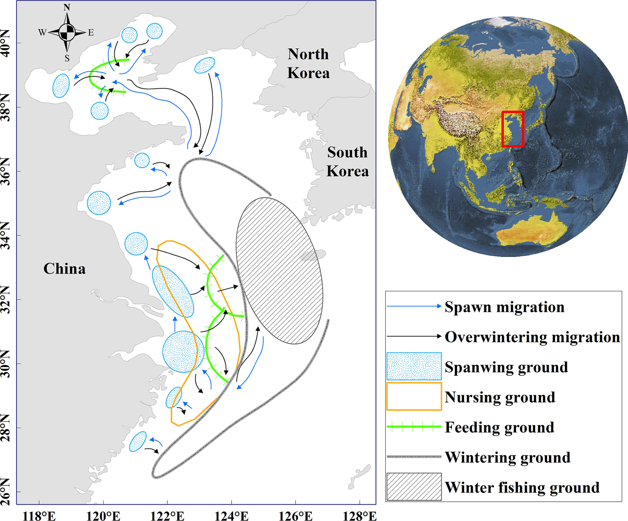
Figure 1 Study area of small yellow croaker. The slash-shaded area indicates the location of potential winter fishing grounds for small yellow croaker.

Fishery data

Monthly catch data are collected by trawling fishery statistics for the period 1971–1982, which comprehensively reflect the small yellow croaker resources in the Bohai Sea, Yellow Sea, and East China sea (hereafter referred to as “the China Seas”). The catch data were recorded by fishing areas with catch and numbers of nets covering a total of 266 fishing areas. Each fishing area consists of 0.5°×0.5° (latitude × longitude); the location of the latitude and longitude of each fishing area was described as the central point.

Winter data (January) were used to explore the distribution of small yellow croaker during the overwintering period, including 554 records in 140 fishing areas with distributions ranging from 26°N–38°N to 120°E–128°E. A total of 505 records in 139 fishing areas from 1971 to 1981 were used to construct the model, and data in 1982 (49 records in 49 fishing areas) were used for model validation.

Generally, CPUE is regarded as an indicator of fish abundance due to its positive correlation with the availability of fishery resources in fishing grounds (Sakurai et al., 2000; Yu et al., 2018; Liu et al., 2020), and in this study, the index associated with CPUE was used to represent the abundance of small yellow croaker. CPUE data for each fishing area was calculated by dividing the total catch by the number of nets, in kg/net.

Environmental data

(1) Environmental variables

Monthly environmental data included surface current velocity (SCV) derived from meridional velocity (V) and zonal velocity (U), sea surface salinity (SSS), and sea surface temperature (SST). SCV is derived from meridional velocity (V) and zonal velocity (U), and the equation of SCV (1) is shown below:

$\begin{array}{ll}SC{V}_{ij}=\sqrt{V_{ij}^2+U_{ij}^2}& (1)\end{array}$

where SCV_ij is the surface current velocity of grid j in year i; V_ij is the meridional velocity of grid j in year i; and U_ij is the zonal velocity of grid j in year i.

The data for 1971–1992 from Simple Ocean Data Assimilation (SODA) v3.3.1 were downloaded from the APDRC data at a spatial resolution of 0.5° ×0.5° (latitude × longitude), and 1993–2020 data were obtained from the Copernicus Marine Service at a spatial resolution of 0.25°×0.25° (latitude × longitude). Submarine elevation data were derived from the ETOPO1 Global Relief Model at a resolution of 1/60° (Table 1). All data were resampled into a 0.1° ×0.1° resolution (latitude × longitude) for consistent spatial resolution.

TABLE 1

Table 1 Environmental data used for research and model construction.

(2) Climate indices

The monthly mean climate indices are from online public datasets and previous literature reports. According to previous literature reports, winter is the most intense period of climate activities, significantly affecting the regional environment. In this study, the PDO, NPGO, AOI, and AMO were used to explore the effects of climate change on fishing ground variations (Table 2).

TABLE 2

Table 2 Climate index used for subsequent analysis.

(3) IPCC-RCP scenarios

The monthly mean environmental conditions in the future (2040–2050 and 2090–2100) were downloaded from a public dataset (https://www.bio-oracle.org). Max depth data from Bio-ORACLE (ocean rasters for analysis of climate and environment), including the temperature, salinity, and surface current velocity of RCP 2.6, RCP4.5, RCP6.0, and RCP8.5, were used to predict the distribution in the future (Lennert et al., 2012; Assis et al., 2018). Rasters were assembled at a resolution of 0.083°×0.083° (latitude × longitude), and were resampled into a 0.1°×0.1° resolution (latitude × longitude) for consistent spatial resolution.

Winter fishing ground indices

To describe the abundance of small yellow croaker under a uniform standard and to observe the winter variation, a Winter Fishing ground Abundance Index (WFAI) was developed to represent the abundance of small yellow croaker qualitatively. The catch and the number of nets in each fishing area were used to calculate the abundance index, and the equation of WFAI (2) is shown below:

$\begin{array}{ll}g\left(WFA{I}_{ij}\right)=\text{ln}\left(CPU{E}_{ij}+1\right)& (2)\end{array}$

The region with WFAI higher than 5 is regarded as winter fishing ground hotspots and could be considered to have a higher occurrence probability of small yellow croaker in winter. The area of winter fishing ground hotspots (WFHA) was calculated as an index to measure the variation of annual dynamic fishing ground in winter. The calculation formula of WFHA (3) is as follows:

$\begin{array}{ll}WFH{A}_i={\displaystyle {\sum }_{j=1}^{N_i}{S}_j}& (3)\end{array}$

where N_i is the grid number of WFAI > 5 in the winter fishing ground in year i; S_j is the size of grid j at 0.1° × 0.1° (latitude × longitude) resolution.

The location of potential winter fishing ground was delineated based on the predicted WFAI distribution. The annual mean values of SST, SSS, and SCV in potential winter fishing ground were calculated separately to represent the environmental condition fluctuations. WFHA and the mean value of WFAI in potential winter fishing ground are used to describe the annual variation of small yellow croaker.

The hotspots center is the center of gravity of hotspots, which is used to indicate the location of winter fishing ground hotspots. In this study, the center of hotspots is obtained by the Mean Center Tool of ArcGIS 10.7.

Develop prediction models for WFAI

A total of 45 combinatorial GLMs, GAMs, and RFs were simulated by incrementally adding variables. The model was constructed with the Marine Geospatial Ecology Tool (MGET) of ArcGIS 10.7, an additional program that applies advanced analytical methods (Roberts et al., 2010). Environmental data [SSS, SST, SCV, and depth (DE)] were used as predictive variables to predict the WFAI distribution of small yellow croaker, and environmental variables were gradually added to the models. The variable inflation factors (VIFs) were examined to determine whether these environmental variables have multi-collinearity, the results show that no variable has a VIF value greater than 5, and the VIF of SSS, SST, SCV, and DE were 2.40, 2.06, 1.80, and 1.80, respectively.

GAMs and GLMs were constructed using the “mgcv” package and “glm” package, respectively. (Wood, 2006). The equations for GAM(4) and GLM(5) are as follows:

$\begin{array}{ll}g\left(Y\right)=\alpha +{\displaystyle {\sum }_{i=1}^n{F}_i\left(X_i\right)+ϵ}& (4)\end{array}$

$\begin{array}{ll}g\left(Y\right)=\alpha +{\displaystyle {\sum }_{i=1}^n\beta \left(X_i\right)+ϵ}& (5)\end{array}$

where g is the link function that constructs the relationship between the response variable and predictor variables, Y is the response variable (WFAI), X_i is the predictor variable (SSS, SST, SCV, and DE), n is the number of variables, F_i is the smoothing function for predictor X_i, α is the intercept, β is the model constant, and ϵ is the random error (Guisan et al., 2002; Wood, 2006).

RF is an ensemble learning method that uses multiple decision trees; usually, a number of trees are trained from the original decision tree (Breiman, 2001). The random forest algorithm is as follows (Liaw and Wiener, 2002): firstly, draw n_tree bootstrap samples from the original data; secondly, for each of the bootstrap samples, grow an unpruned classification or regression tree, with the following modification: at each node, rather than choosing the best split among all predictors, randomly sample m_try of the predictors and choose the best split from among those variables; thirdly, aggregate these trees’ information to predict new data. In this study, n_tree was set to 500 and a “random forest” software package was used to build RF models.

The GLM, GAM, and RF models were developed using monthly raster data from 1971 to 1981 and then predicted the WFAI in 1982; the model performance was evaluated by comparing the predicted and actual values. Increasing variables incrementally caused changes in the explanatory rate and the Akaike information criterion (AIC) in the GAMs and GLMs, and deviance was explained in RFs. Therefore, the highest deviance explained and the lowest AIC (Johnson and Omland, 2004) were used to seek out the best GAM and GLM, and choose RF with the highest deviance explained.

Detection method for regime shift

The Sequential t-test Analysis of Regime Shift (STARS) was applied to detect trends and step changes within the time series data, including WFAI, WFHA, SST, SSS, SCV, and climate indices (Rodionov, 2004). STARS results are determined by significance level (P), cutoff length (L), and the Huber’s weight parameter (H), which controls the magnitude and scale of the regimes and the weights assigned to the outliers. In this study, the STARS cutoff length was set to 10, the Huber’s weight parameter to 2, and the significance level to 0.1, consistently. In addition, the Cumulative sum (CuSum) of the anomalies was used to denote the trend of all exponential time series (Beamish et al., 1999).

Results

Optimal prediction model for WFAI

The best-performing GAM, GLM, and RF models are shown in Table 3. In GAM, the best-performing model has three significant predictor variables (SCV and SST with p < 0.001 and DE with p < 0.01) with the lowest AIC (2010.26) and the highest deviance explained (34.7%). For GLM, the final selected model with three significant predictors (SCV and SST with p < 0.001 and DE with p < 0.01) had the lowest AIC (2,116.40) and a high explained variance (15.80%). In RF, the predictive model containing four variables was selected, with deviance explained at 37.7%. Compared with the three models, the RF model has the highest explanation.

TABLE 3

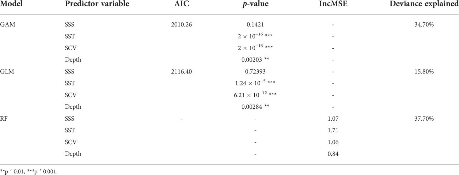
Table 3 GAM, GLM, and RF models included predictor variables, AIC, p-value, IncMSE, and deviance explained.

Figure 2 shows the comparison of actual WFAI and RF, GAM, and GLM model prediction results in 1982. The predicted hotspot distributions of RF, GAM, and GLM are consistent with the actual values, indicating that the prediction performance was reasonable. However, GAM predictions show high values in nearshore waters that are not consistent with reality. Among the validation data, 30.61% were underestimated and 12.24% were overestimated in GLM predictions. Figure 3 shows that RF was the best model by comparing the relationships between the predicted and actual WFAI for each selected model. The RF-based model showed the highest correlation (R² = 0.54, p < 0.01), which was greater than those from GAM (R² = 0.47, p < 0.01) and GLM (R² = 0.29, p < 0.01). Therefore, the RF model was selected as the most suitable model for subsequent prediction.

FIGURE 2

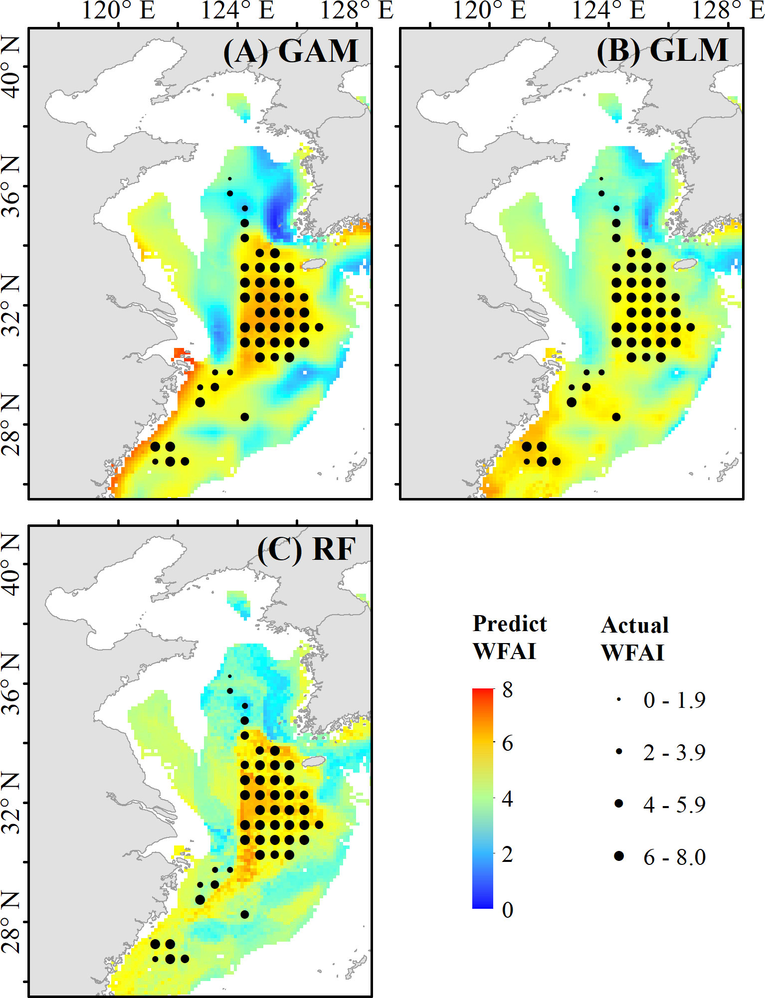
Figure 2 Comparison of the predicted distribution and the actual WFAI values in 1982. Distribution map in (A) is the prediction result of the generalized additive model (GAM), (B) is the prediction result of the generalized linear model (GLM), and (C) is the prediction result of the random forest model (RF).

FIGURE 3

Figure 3 Validation of predicted and actual WFAI values of GAM (A), GLM (B), and RF (C) in 1982.

Spatial distribution of WFAI

The final predicted WFAI of small yellow croaker from 1971 to 2020 (Figure 4) was produced by using the RF model; spatial variation showed that in the past 50 years, WFHA has gradually decreased, and the WFHA in 2020 is significantly lower than in 1971. It was shown that winter fishing ground hotspots mainly concentrated in 30°N–35°N, 123°E–127°E with annual variations; these regions may become a potential winter fishing ground for small yellow croaker. In the Yellow Sea, the range of hotspots gradually decreased, with the most extensive distribution in the 1970s. The smallest range of hotspots occurred in 1985, followed by 1992. After the 1990s, the northern boundary of the hotspots barely exceeded 35°N. In the East China Sea, the hotspot range was also widely distributed in the 1970s, decreasing from the 1980s to the 1990s and increasing after the 2000s. While the smallest area appeared in 1972, the largest area appeared in 1989. In addition, the hotspots in the Yellow Sea and the East China Sea were contiguous in the 1970s and 1980s, and from the 1990s, the winter fishing ground tended to divide into two parts. There are also only a few years with hotspots distributed in the eastern part of Jeju island, which are 1971–1975, 1981, and 1991.

FIGURE 4

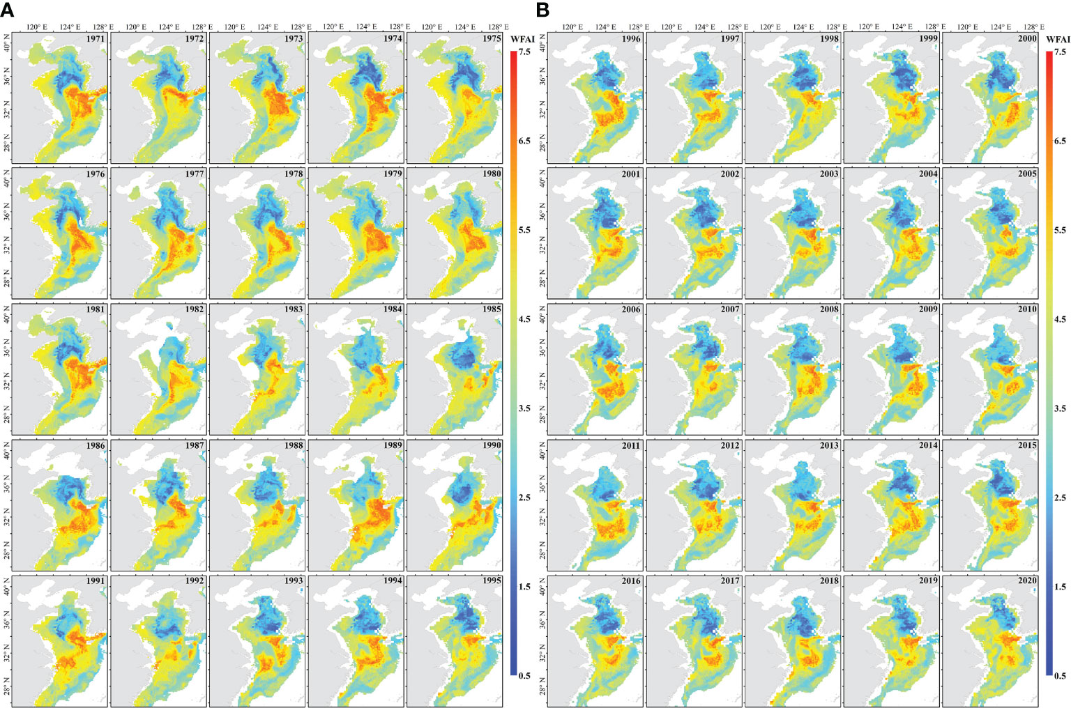
Figure 4 The annual WFAI distribution map of small yellow croaker in the China Seas during 1971–1995 (A) and 1996–2020 (B).

Temporal variations in winter fishing grounds

Winter fishing grounds of small yellow croaker were defined as shown in Figure 1, which are distributed in the offshore area between 29°N and 35°N according to the average distribution of WFAI from 1971 to 2020.

The mean values of WFAI, WFHA, SSS, SST, and SCV of winter fishing grounds were calculated annually. WFAI and WFHA displayed a decreasing trend in fluctuation, while SSS, SST, and SCV had a dynamic increase (Figures 5, 6). The dynamic trends of WFAI and WFHA are almost identical, with a sudden drop in 1985 and then rise again, followed by another dip in 1992 and then fluctuating changes. Maximum and minimum values occurred in 1973 (5.39 for WFAI; 123,328 km² for WFHA) and 1985 (4.24 for WFAI; 50,896 km² for WFHA), respectively (Figures 5A, B).

FIGURE 5

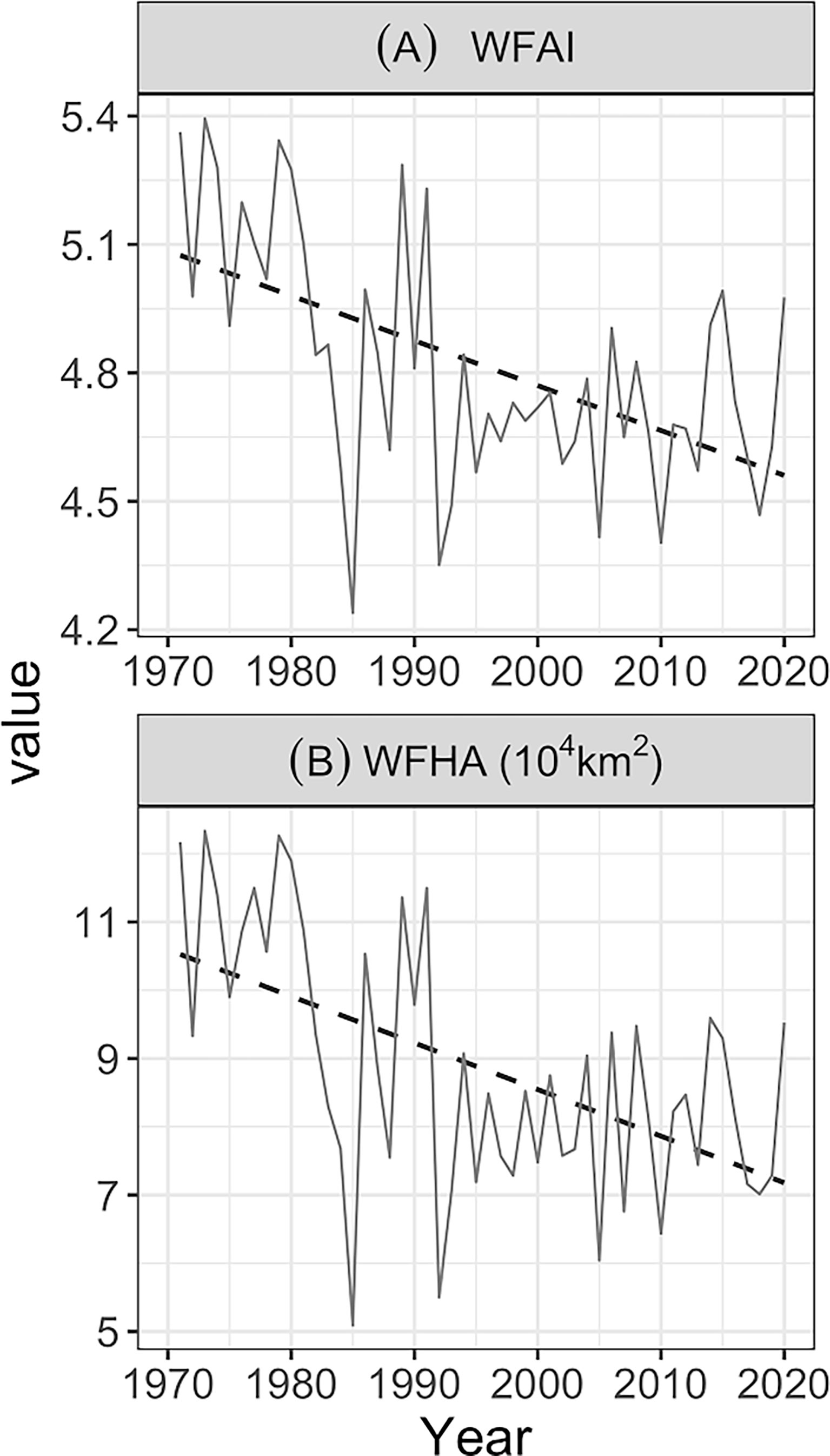
Figure 5 Annual variations (solid lines) of WFAI (A) and WFHA (B) from 1971 to 2020. The black dashed lines represent linear trends.

FIGURE 6

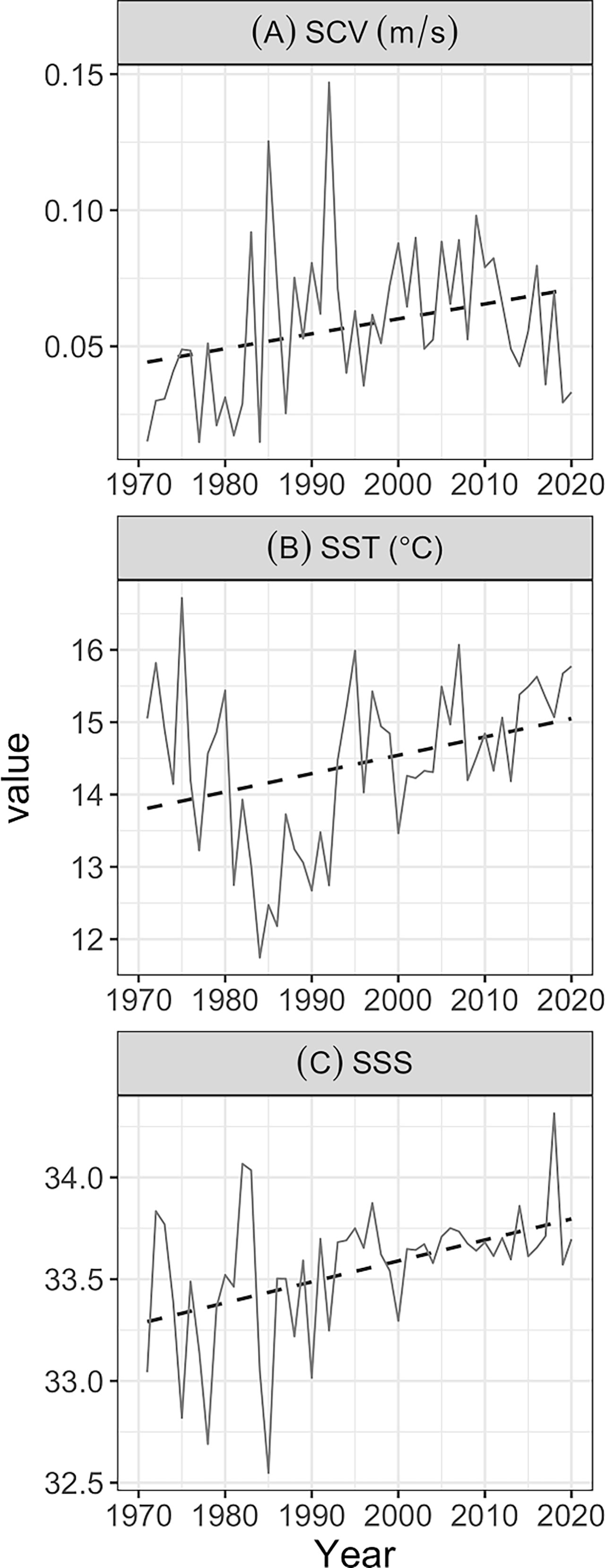
Figure 6 Annual variations (solid lines) of SCV (A), SST (B), and SSS (C) in winter fishing grounds from 1971 to 2020. The black dashed lines represent linear trends.

Surface current velocity shows the opposite trend, which was extremely high in 1985 and 1992 and decreased in the middle years (Figure 6A). A correlation analysis revealed that WFAI (r = 0.61, p < 0.01) and WFHA (r = 0.62, p < 0.01) were negatively correlated with SCV. SST and SSS remained low during this period, with a minimum value in 1985 (Figures 6B, C).

Climate-induced variations in WFAI

STARS analysis results show that the mean values of WFAI highlighted regime shifts with significant decreasing trends during 1981/1982 and 1991/1992, so was WFHA, which displayed the same regime shift trends in 1981/1982 and 1991/1992 (Figures 7A, B). SSS shows regime shifts with increasing trends in 1992/1993 and SCV in 1984/1985 separately (Figures 7C, E). SST highlighted that regime shifts decreased in 1980/1981 and increased in 1992/1993 (Figure 7D). The climatic indices showed evident decadal variability from 1971 to 2020 with regime shifts in 1976/1977 and 1988/1989 for PDO (Figure 7F), increasing shift in 1997/1998 and decreasing in 2013/2014 for NPGO (Figure 7G), and only one increased regime shift in 1988/1989 for AOI, and 1994/1995 for AMO (Figures 7H, I).

FIGURE 7

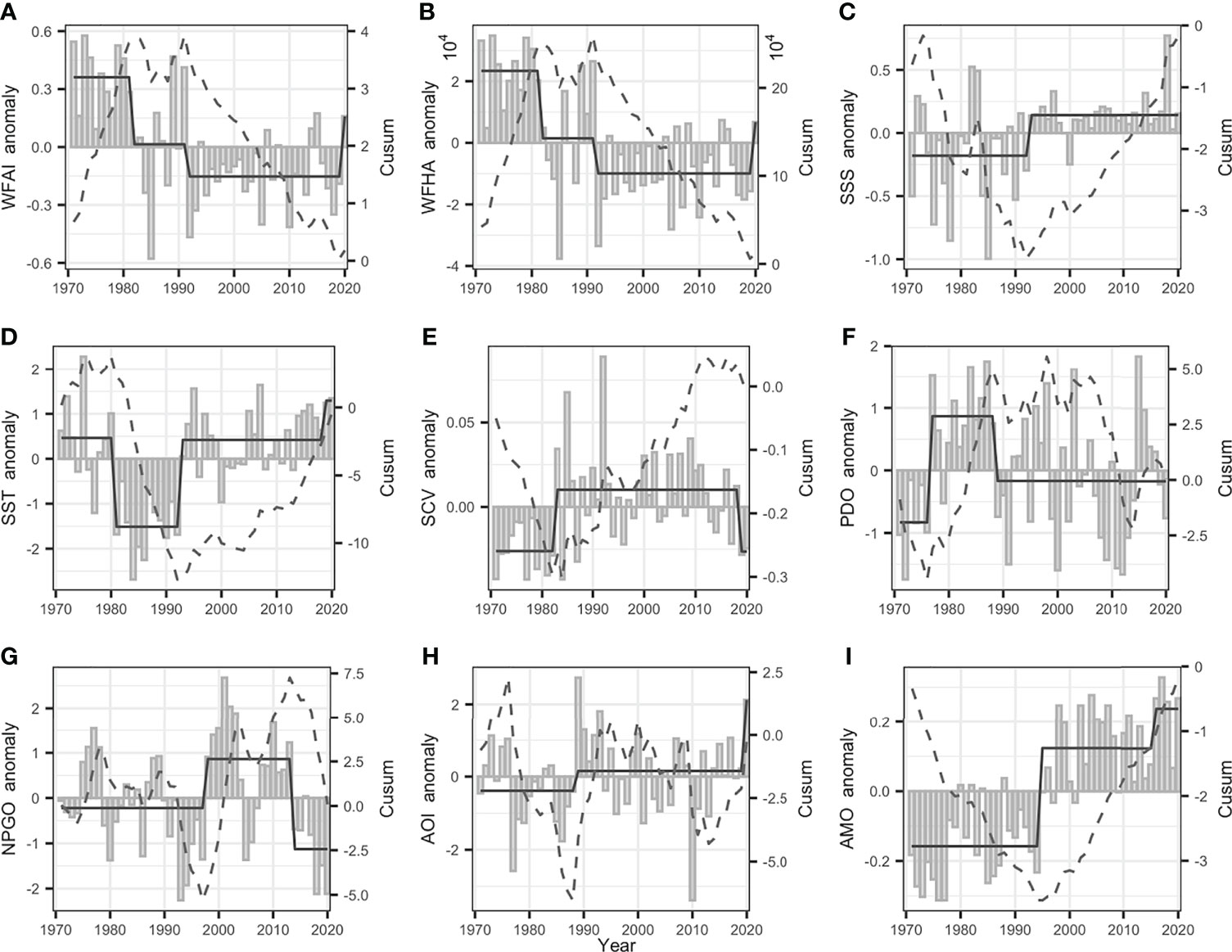
Figure 7 The gray bars represent annual anomalies of WHAI (A), WFHA (B), SSS (C), SST (D), SCV (E), PDO (F), NPGO (G), AOI (H), AMO (I), and the solid and dashed lines represent the cumulative sum of SRSD-detected anomalies and regime shifts (CuSum).

Future prediction of WFAI

Based on different greenhouse gas emissions in 2040–2050 and 2090–2100, WFAI distribution of small yellow croaker in the mid- and late 21st century under the RCP2.6 and RCP8.5 scenarios with the highest and lowest gas emissions is shown in Figure 8.

FIGURE 8

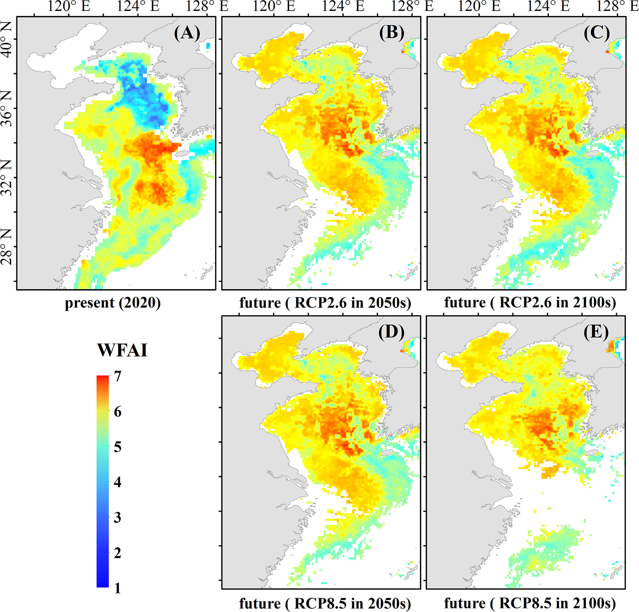
Figure 8 Present and two scenarios based on future predicted WFAI of small yellow croaker. (A) Present distribution in 2020, (B) future distribution in RCP2.6 (2050s), (C) future distribution in RCP2.6 (2100s), (D) future distribution in RCP8.5 (2050s), and (E) future distribution in RCP8.5 (2100s).

The RCP2.6 scenario prediction (Figures 8B, C) shows that the hotspot area shifted significantly northward in the mid-to-late 21st century compared to 2020 (Figure 8A), with the southern boundary moving from 30°N to 33°N, the western edge moving from 123°E to 121°E, the hotspot region moving from the East China Sea to the Yellow Sea, and the WFHA increasing significantly from 2020. At the end of the 21st century, the northern boundary of hotspots shifts southward and becomes more concentrated than in the middle of the century.

In the RCP8.5 scenario predictions (Figures 8D, E), the hotspots of winter fishing grounds also shifted northward in the mid-to-late 21st century. The dynamics in the 2050s are similar to RCP2.6, with the hotspots in the East China Sea moving to the Yellow Sea, and with the southern boundary near 35°N. At the end of the 21st century, hotspots became smaller and more concentrated, mainly between 122°E–124°E and 34°N–36°N in the Yellow Sea, with fewer hotspots appearing at 125°E–126°E.

Discussion

Model performance

In this research, a series of SDMs (GLMs, GAMs, and RFs) were simulated based on WFAI and environmental variables. The RF model was selected to be the optimal prediction model for small yellow croaker in the overwintering period with the highest deviance explained at 37.70%. GAMs were suboptimal compared with GLMs, which had the lowest deviance explained at 15.80%. We also compared the prediction performance of three model types. The results showed that the RF model had the highest correlation between predicted and actual WFAI, slightly higher than GAM and nearly two times higher than GLM. Moreover, GAM predictions showed unexpectedly high values in nearshore waters where there were overestimated and GLM predictions underestimated approximately 30% of the whole area of hotspots compared with RF. GLMs are based on linear multiple regression and can deal with presence–absence data. GAMs are similar to GLMs and can handle nonlinear responses using quadratic, cubic, or other smoothers. Generally, the relationship between species distribution and environmental variables could be nonlinear. Our results also indicated that GAMs had better performance than GLMs. Several studies have demonstrated that machine learning approaches (e.g., RFs, SVMs, and ANNs) could outperform traditional regression approaches (e.g., GLMs and GAMs) (De Clercq et al., 2015; Luan et al., 2018; Catucci and Scardi, 2020). Among the six candidate methods (GLMs, GAMs, RTs, RFs, ANNs, and SVMs) applied to Japanese Spanish mackerel, the higher predictive quality of four machine learning models (RTs, ANNs, RFs, and SVMs) has also been expressed over GLMs and GAMs (Li et al., 2015). Machine learning models have advantages in handling non-linear relationships and could avoid overfitting the training data (Luan et al., 2020). Machine learning approaches can provide well-controlled variable selection and coefficient estimation; hence, their prediction performance may exceed conventional regression models. It would see machine learning approaches becoming more and more popular in SDMs because of their advantages in prediction.

Impact of environmental variables on the WFAI of small yellow croaker

The 50-year average distribution map of small yellow croaker in winter was generated combined with an isoline map of SST and DE (Figure 9). The results showed that the hotspots of small yellow croaker winter fishing grounds were mainly distributed between 11°C and 16°C isotherms and between 50-m and 100-m isobaths, similar to previous studies which described a suitable temperature range between 8°C and 18°C and a depth between 50 m and 80 m (Lin, 1987; Liu et al., 2020b). It has been reported that small yellow croaker had a higher occurrence probability of between 11.5°C and 16.2°C and a higher abundance of between 15.1°C and 16.7°C in winter (Liu and Cheng, 2018). These indicated that small yellow croaker could tolerate lower temperatures under 11°C, but more concentrated on suitable winter fishing grounds. The suitable depth range in our study was between 50 m and 100 m, a little larger than previous studies. This may be related to the benefit from remote sensed data that provide a broader range of environmental data.

FIGURE 9

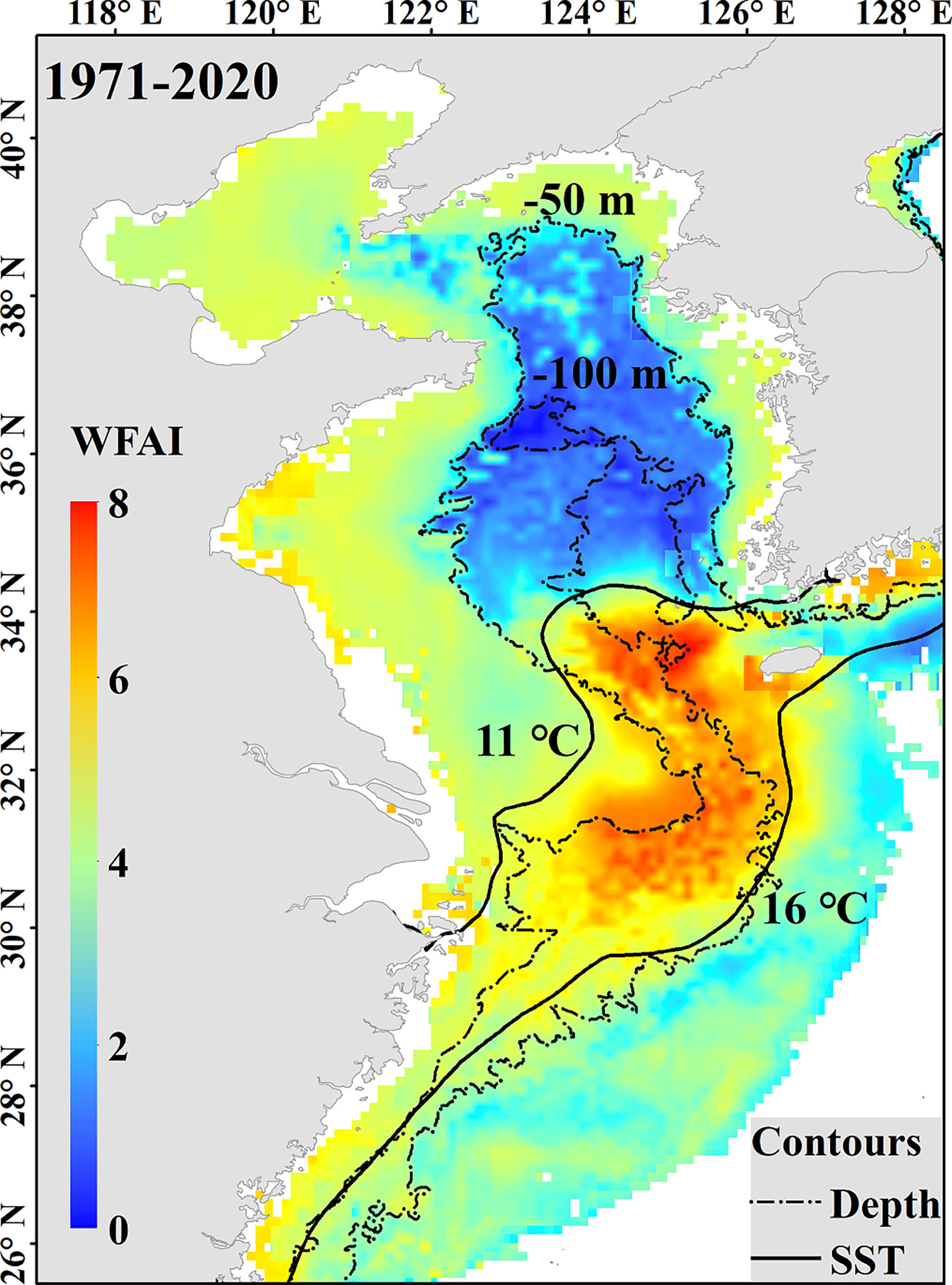
Figure 9 The 50-year average WFAI distribution map of small yellow croaker with environmental conditions (the dashed lines represent isobaths, and the solid lines represent isotherms).

The decadal distribution map emphasized the impact of environmental variables on winter fishing grounds. It has shown that temperature and salinity front jointly determine the boundary of hotspots of WFAI (Figure 10). The potential winter fishing grounds of small yellow croaker are affected by the Yellow Sea Warm Current (YSWC) and the coastal currents. The YSWC is believed to be the only mean flow that brings warm and saline water into the interior of the Yellow Sea and forms warm and saline tongue structures in winter (Ma et al., 2006). Furthermore, freshwater discharge from the Yangtze River also affects the salinity of the East China Sea (Delcroix and Murtugudde, 2002). This complex current system generated temperature and salinity fronts, which limited the boundary of winter fishing ground of small yellow croaker. The distribution of WFAI showed a strong relationship with fronts, with a clear boundary that was hardly north than 35°N. The shape of the small yellow croaker winter fishing ground hotspots is also strongly associated with temperature fronts and salinity fronts.

FIGURE 10

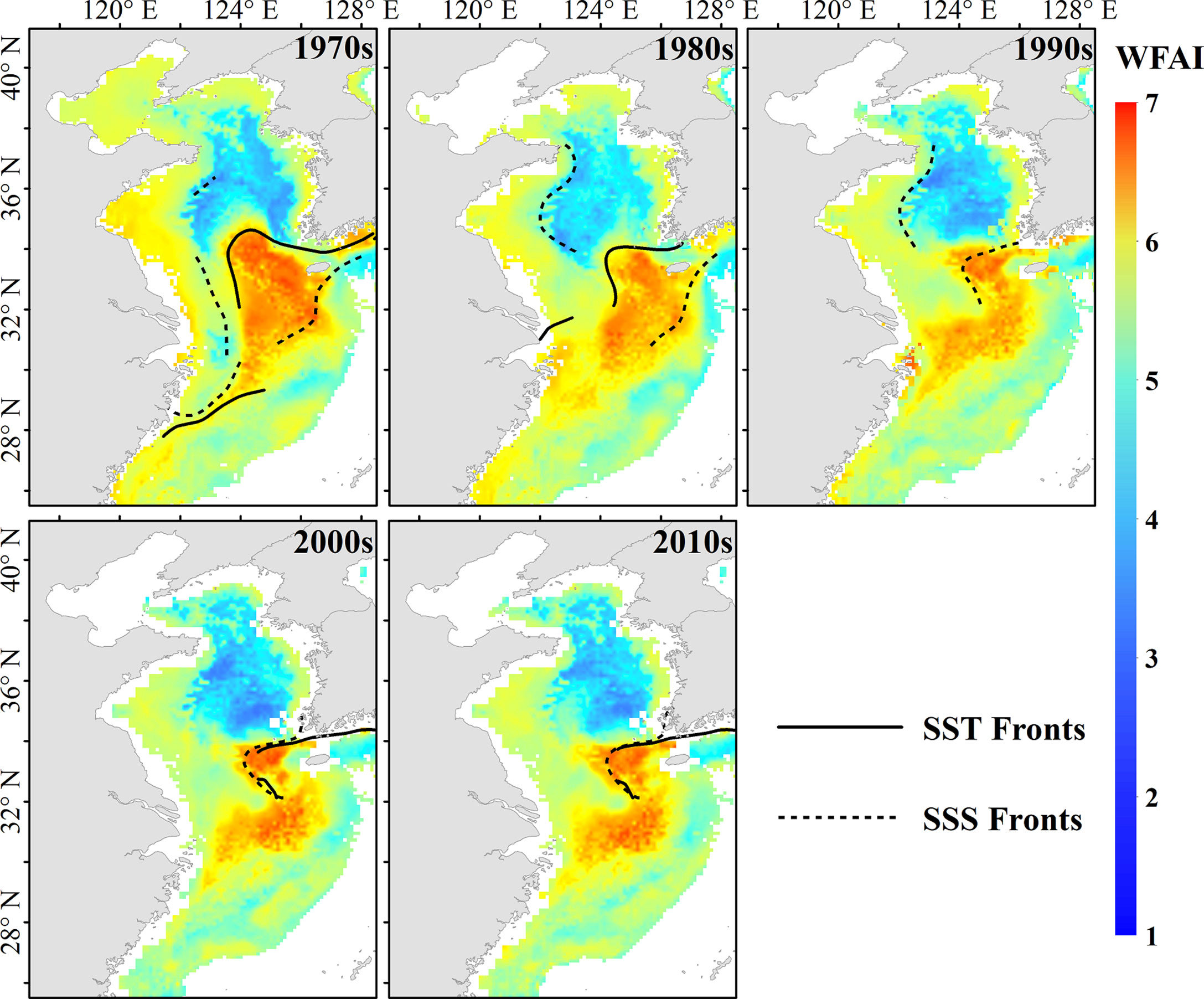
Figure 10 The decadal average WFAI distribution map of small yellow croaker with environmental variable in front (the black solid line is the front of decadal average temperature, and the dashed line is the front of decadal average salinity).

The long-term change of mean WFAI showed a decreasing trend in the last 50 years, similar to the WFHA (Figure 6). Similar results were described in the work of Han et al. (2020), which found that the biomass of small yellow croaker in the winter period showed a marked decline, but the study was only conducted between 2001 and 2017, while the long-term changes of environmental variables showed an increasing trend (Figure 6), indicating that the environmental changes may have a negative effect on the WFAI and the WFHA of small yellow croaker. The STARS analyses for mean values of WFAI and WFHA in winter fishing grounds suggested that regime shifts took place in 1981/1982 and 1991/1992. SST showed regime shifts in 1980/1981 and 1992/1993, while SSS showed regime shifts in 1992/1993 and SCV in 1984/1985. The almost synchronous regime shifts also indicated that the potential winter fishing grounds of small yellow croaker were directly affected by environmental variables. The decadal average anomaly map manifested that the current velocity in the potential winter fishing ground of small yellow croaker was relatively smaller than in other regions (excluding the Kuroshio region) (Figure 11). This may indicate that small yellow croaker prefers gentle areas during winter, which could be related to a lower feeding rate and energy conserved. The small yellow croaker mainly preys on Japanese anchovy, Kammal thryssa, Kishi velvet shrimp, and Mitre squid (Xiao et al., 2019). Due to the limited data, the influence of prey conditions was not involved in this research.

FIGURE 11

Figure 11 Decadal average anomaly map of surface current velocity in 1971–2020.

Effect of climate change on small yellow croaker

The correlation analyses between the annual mean WFAI and environmental variables are detected in Figure 12. WFAI showed a weak relationship with SST and SSS, but a strong negative relationship with SCV (r = −0.61, p < 0.001). The WFAI and WFHA highlighted a significant positive correlation (r = 0.97, p < 0.001); hence, WFHA also showed a strong negative correlation with SCV (r = −0.62, p < 0.001). As for climate indices, PDO highlighted regime shifts in 1976/1977 and 1988/1989, NPGO showed regime shifts in 1997/1998 and 2013/2014, AOI showed a regime shift only in 1988/1989, and AMO showed a regime shift only in 1994/1995. The correlation tests indicated that WFAI and WFHA highlighted a strong negative correlation with AMO (WFAI: r = −0.44, p < 0.01; WFHA: r = −0.46, p < 0.01) and a relatively weak correlation with AOI, NPGO, and PDO (Figure 12). This may imply that AMO had a closer relationship with WFAI and WFHA than AOI, NPGO, and PDO. Previous studies have attributed the decadal variability in the North Pacific to PDO, but recent studies have illustrated that the AMO instead controlled it using long records of observations (Wu et al., 2020). They found that PDO had little relationship with the North Pacific subtropical mode water when the data were extended back to the 1940s, and only after 1978 did the negative correlation appear, which reflected the fact that the warming trend of the mode water coincided with a phase transition of the PDO index from a positive to a negative phase, rather than a robust relationship. Our results also supported this view with a strong correlation between WFAI and AMO and a lower correlation with PDO. Among environmental variables and climate indices, SST and SSS showed relatively strong positive correlations with AMO (r = 0.33, p < 0.05 for SST; r = 0.39, p < 0.05 for SSS), and SCV showed a weak correlation with AMO (r = 0.17, p < 0.1). SST had a positive correlation with SSS (r = 0.34, p < 0.05). This could be related because the salinity and temperature were related to the ocean current in the China Seas (Chen, 2009). From these observations, we proposed a potential process to explain the variations of small yellow croaker in the overwintering period. AMO-based climate regimes led to changes in the Kuroshio Current region through ocean–atmosphere interactions. The Kuroshio Current entered the China Seas, which were located on the western edge of the North Pacific and were affected by the Kuroshio Current and its branches. The potential winter fishing grounds of small yellow croaker were directly affected by the coastal currents and the Yellow Sea Warm Current (YSWC), which was the branch of the Kuroshio Current (Bian et al., 2013). The YSWC brings warm and saline water into the interior of the Yellow Sea (Ma et al., 2006). The abundance of small yellow croaker was directly influenced by the environmental conditions (SST, SSS, and SCV) in winter fishing grounds. Therefore, the long-term changes of WFAI and WFHA were more likely associated with AMO than other climate indices.

FIGURE 12

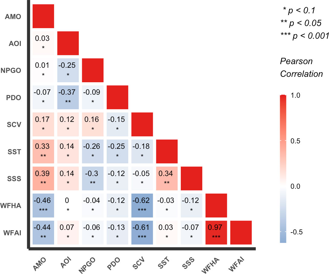
Figure 12 The correlation analyses between the annual mean WFAI, WFHA, mean values of environmental variables, and climate indices.

Future prediction of winter fishing ground change

Based on the optimal prediction model, the decadal distribution maps of hotspots were generated to investigate variations in winter fishing grounds (Figure 10). The decadal distribution maps indicated that the spatial range and area of hotspots tended to be shrinking. Moreover, the winter fishing grounds tended to be divided into two parts, and this trend became more distinct after the 1990s. The boundary of hotspot distribution also changed with time. The north boundary of hotspots moved southward to 34°N after the 1970s, which was also reported by Han et al. (2020). The south boundary of hotspots tended to move northward near 30°N after the 1970s. The east boundary of the north parts of the winter fishing grounds extended eastward to 127°E and the west boundary of the south parts tended to move westward to 123°E. Moreover, the hotspot distribution showed a more concentrated trend though the area became smaller. Our results indicated that the spatial distribution changes in the winter fishing ground of  small yellow croaker were likely to be embodied in the boundary.

We conducted future distribution maps based on two extreme scenarios (RCP2.6 and RCP8.0). The results showed that the distribution of small yellow croaker will move obviously northward and the WFHA will become broader (Figure 8), and the southernmost overwintering districts might become less important to the stock under future climate change. The north boundary of WFHA can reach 40°N, and the south boundary can reach 30°N. The west boundary moves to 118°E, and the east boundary moves to 127°E. The center of the winter fishing ground was also generated to investigate the long-term changes with a focus on hotspots (Figure 13). Results showed that the center of winter fishing ground would distinctly move northward in the 2050s and the 2100s than in 1970–2020 related to 16°C isotherms. Distribution movement driven by climate change has been found in a large number of species (Perry et al., 2005; Last et al., 2011). Thirteen fish species have been newly recorded in the Taiwan Strait beyond their historic range in the South China Sea (Du et al., 2013). The hotspot distribution of hairtail in the East China Sea was found to move north eastward from 1991 to 2011 (Yuan et al., 2017). Many species have been simulated to move poleward under different scenario predictions of climate change (Jones and Cheung, 2015; Morley et al., 2018). These shifts were projected to lead to increases in mid- and high-latitude oceans and decreases in tropical regions (Cheung et al., 2009). All these changes call for the improvement of resource management and conservation.

FIGURE 13

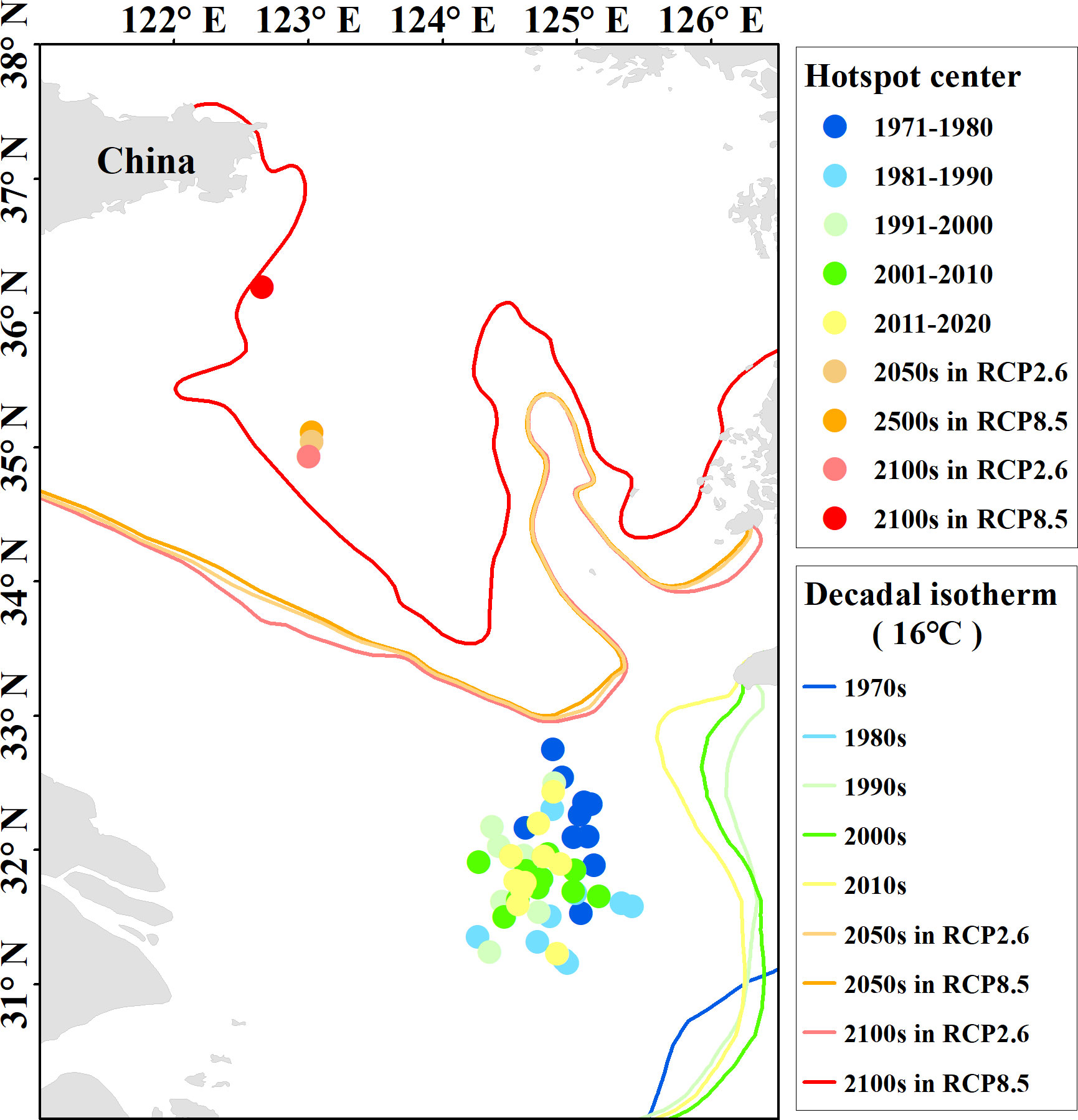
Figure 13 The hotspot center and decadal isotherm from 1971 to 2020 and the future prediction in two RCP scenarios.

Conclusion

Three types of SDMs (GLMs, GAMs, and RFs) of small yellow croaker were developed using WFAI as the response variable and environmental variables as explanatory variables. A comparison of the models revealed that the RF model was the optimal prediction model. Results showed that the WFAI distribution was related to SST, SSS, SCV, and DE, and the winter fishing ground hotspots were mainly distributed between 11°C and 16°C isotherms and between 50-m and 100-m isobaths. The shape of hotspots was strongly affected by temperature fronts and salinity fronts. A long-time scale analysis revealed a decreasing trend in the winter fishing ground hotspots—the northern boundary shifts southward, the southern border shifts northward, and there was a tendency to divide into two parts, gradually. The WFHA has significantly decreased over the past 50 years. WFAI and WFHA highlighted similar regime shift trends, and the distribution of small yellow croaker might be more closely related to AMO than PDO, AOI, and NPGO in winter fishing grounds. Future predictions based on two extreme climate scenarios (RCP2.6 and RCP8.0) indicated that the winter fishing ground hotspots of small yellow croaker would move obviously northward by the end of this century under climate warming. Climate and environmental changes could have far-reaching effects on changes in small yellow croaker fisheries.

Data availability statement

The raw data supporting the conclusions of this article will be made available by the authors, without undue reservation.

Author contributions

RZ performed data analyses, model construct, and wrote the paper. YL conceived the idea for the study, analyses, and edited the manuscript. HT edited part of the figures. SL and XX extracted part of environmental data. KZ edited the manuscript. All authors listed have made a direct and substantial contribution to this work. All authors read and approved the final manuscript.

Acknowledgments

This study was supported by the National Key R&D Program of China (2018YFD0900902). The study benefited from statistics on fishing vessels from the Yellow Sea Fisheries Research Institute and the East China Sea Fisheries Research Institute for the period 1971–1982. We are particularly grateful to the Yellow Sea Fisheries Research Institute and the East China Sea Fisheries Research Institute of the Chinese Academy of Fishery Sciences for their support.

Conflict of interest

The authors declare that the research was conducted in the absence of any commercial or financial relationships that could be construed as a potential conflict of interest.

Publisher’s note

All claims expressed in this article are solely those of the authors and do not necessarily represent those of their affiliated organizations, or those of the publisher, the editors and the reviewers. Any product that may be evaluated in this article, or claim that may be made by its manufacturer, is not guaranteed or endorsed by the publisher.

References

Assis J., Tyberghein L., Bosch S., Verbruggen H., Serrão E. A., De Clerck O. (2018). Bio-ORACLE v2.0: Extending marine data layers for bioclimatic modelling. Glob. Ecol. Biogeogr. 27, 277–284. doi: 10.1111/geb.12693

CrossRef Full Text | Google Scholar

Bao B., Ren G. (2014). Climatological characteristics and long-term change of SST over the marginal seas of China. Cont. Shelf. Res. 77, 96–106. doi: 10.1016/j.csr.2014.01.013

CrossRef Full Text | Google Scholar

Beale C., Lennon J. (2012). Incorporating uncertainty in predictive species distribution modelling. Philos. Trans. R. Soc Lond. B. Biol. Sci. 367, 247–258. doi: 10.1098/rstb.2011.0178

CrossRef Full Text | Google Scholar

Beamish R. J., Noakes D. J., McFarlane G. A., Klyashtorin L., Ivanov V. V., Kurashov V. (1999). The regime concept and natural trends in the production of pacific salmon. Can. J. Fish. Aquat. Sci. 56, 516–526. doi: 10.1139/f98-200

CrossRef Full Text | Google Scholar

Bian C., Jiang W., Greatbatch R. J. (2013). An exploratory model study of sediment transport sources and deposits in the bohai Sea, yellow Sea, and East China Sea. J. Geophys. Res. Ocean. 118, 5908–5923. doi: 10.1002/2013JC009116

CrossRef Full Text | Google Scholar

Breiman L. (2001). Random forests. Mach. Learn. 45, 5–32. doi: 10.1023/A:1010933404324

CrossRef Full Text | Google Scholar

Brown S. K., Buja K. R., Jury S. H., Monaco M. E., Banner A. (2000). Habitat suitability index models for eight fish and invertebrate species in casco and sheepscot bays, Maine. North Am. J. Fish. Manage. 20, 408–435. doi: 10.1577/1548-8675(2000)020<0408:HSIMFE>2.3.CO;2

CrossRef Full Text | Google Scholar

Bureau of fishery of Ministry of Agriculture of China.China Fishery statistical yearbook. (1970-2019) (Beijing: China Agriculture Press).

Google Scholar

Catucci E., Scardi M. (2020). A machine learning approach to the assessment of the vulnerability of posidonia oceanica meadows. Ecol. Indic. 108, 105744. doi: 10.1016/j.ecolind.2019.105744

CrossRef Full Text | Google Scholar

Chavez F., Ryan J., Lluch-Cota S., Niquen M. (2003). From anchovies to sardines and back: multidecadal CHANGE in the pacific ocean. Science 299, 217–221. doi: 10.1126/science.1075880

CrossRef Full Text | Google Scholar

Chen C. T. A. (2009). Chemical and physical fronts in the bohai, yellow and East China seas. J. Mar. Syst. 78, 394–410. doi: 10.1016/j.jmarsys.2008.11.016

CrossRef Full Text | Google Scholar

Cheng J., Lin L., Jiang Y., Yuan X., Li J., Gao T. (2004). Effects of summer close season and rational utilization on redlip croaker (Larimichthys polyactis beeker)resources in the East China Sea region. J. Fish. China 11, 554–560. doi: 10.3321/j.issn:1005-8737.2004.06.012

CrossRef Full Text | Google Scholar

Cheung W. W. L., Lam V. W. Y., Sarmiento J. L., Kearney K., Watson R., Pauly D. (2009). Projecting global marine biodiversity impacts under climate change scenarios. Fish. Fish. 10, 235–251. doi: 10.1111/j.1467-2979.2008.00315.x

CrossRef Full Text | Google Scholar

Chiu T.-Y., Chiu T.-S., Chen C.-S. (2017). Movement patterns determine the availability of Argentine shortfin squid illex argentinus to fisheries. Fish. Res. 193, 71–80. doi: 10.1016/j.fishres.2017.03.023

CrossRef Full Text | Google Scholar

Collins M., Knutti R., Arblaster J., Jean-Louis Dufresne T. F., Pierre Friedlingstein X. G., William J., Gutowski T. J. Jr, et al (2013). Long-term Climate Change: Projections, Commitments and Irreversibility. In: Climate Change 2013: The Physical Science Basis. Contribution of Working Group I to the Fifth Assessment Report of the Intergovernmental Panel on Climate Change. [Stocker, T.F., D. Cambridge, United Kingdom and New York, NY, USA.: Cambridge University Press.

Google Scholar

De Clercq E. M., Leta S., Estrada-Peña A., Madder M., Adehan S., Vanwambeke S. O. (2015). Species distribution modelling for Rhipicephalus microplus (Acari: Ixodidae) in Benin, West Africa: Comparing datasets and modelling algorithms. Prev. Vet. Med. 118, 8–21. doi: 10.1016/j.prevetmed.2014.10.015

CrossRef Full Text | Google Scholar

Delcroix T., Murtugudde R. (2002). Sea Surface salinity changes in the East China Sea during 1997–2001: Influence of the Yangtze river. J. Geophys. Res. Ocean. 107, SRF 9–1-SRF 9-11. doi: 10.1029/2001JC000893

CrossRef Full Text | Google Scholar

Drinkwater K. F., Miles M. W., Medhaug I., Otterå O. H., Kristiansen T., Sundby S., et al. (2013). The Atlantic multidecadal oscillation: Its manifestations and impacts with special emphasis on the Atlantic region north of 60°N. J. Mar. Syst. 133. doi: 10.1016/j.jmarsys.2013.11.001

CrossRef Full Text | Google Scholar

Du J., William W. L. C., Chen B., Qiulin Z., Shengyun Y., Guanqiong Y. (2013). Progress and prospect of climate change and marine biodiversity. Biodivers. Sci. 20, 745–754. doi: 10.3724/SP.J.1003.2012.10051

CrossRef Full Text | Google Scholar

Elith J., Leathwick J. R. (2009). Species distribution models: Ecological explanation and prediction across space and time. Annu. Rev. Ecol. Evol. Syst. 40, 677–697. doi: 10.1146/annurev.ecolsys.110308.120159

CrossRef Full Text | Google Scholar

Fishery Bureau of Ministry of Agriculture (1987). The fisheries resources survey and divisions in the East China Sea region (Shanghai: East China Normal University Press).

Google Scholar

Friedman J. H. (1991). Multivariate adaptive regression splines. Ann. Stat. 19, 1–67. doi: 10.1214/aos/1176347963

CrossRef Full Text | Google Scholar

Grubbs R. D., Musick J. A., Conrath C. L., Romine J. G. (2007). Long-term movements, migration, and temporal delineation of a summer nursery for juvenile sandbar sharks in the Chesapeake bay region. Am. Fish. Soc Symp. Ser. 50, 87–107.

Google Scholar

Guerra T. P., Santos J. M. F. F., Pennino M. G., Lopes P. F. M. (2021). Damage or benefit? how future scenarios of climate change may affect the distribution of small pelagic fishes in the coastal seas of the americas. Fish. Res. 234. doi: 10.1016/j.fishres.2020.105815

CrossRef Full Text | Google Scholar

Guisan A., Edwards T. C., Hastie T. (2002). Generalized linear and generalized additive models in studies of species distributions: setting the scene. Ecol. Modell. 157, 89–100. doi: 10.1016/S0304-3800(02)00204-1

CrossRef Full Text | Google Scholar

Guisan A., Thuiller W. (2005). Predicting species distribution: Offering more than simple habitat models. Ecol. Lett. 8, 993–1009. doi: 10.1111/j.1461-0248.2005.00792.x

CrossRef Full Text | Google Scholar

Han Q., Grüss A., Shan X., Jin X., Thorson J. (2020). Understanding patterns of distribution shifts and range expansion/contraction for small yellow croaker (Larimichthys polyactis) in the yellow Sea. Fish. Oceanogr. 30. doi: 10.1111/fog.12503

CrossRef Full Text | Google Scholar

Hu W., Du J., Su S., Tan H., Yang W., Ding L., et al. (2022). Effects of climate change in the seas of China: Predicted changes in the distribution of fish species and diversity. Ecol. Indic. 134, 108489. doi: 10.1016/j.ecolind.2021.108489

CrossRef Full Text | Google Scholar

Jin X., Zhao X., Meng T. (2005). Biological resource and habitation environment of the bohai and yellow Sea (Beijing, China: Science Press).

Google Scholar

Johnson J. B., Omland K. S. (2004). Model selection in ecology and evolution. Trends Ecol. Evol. 19, 101–108. doi: 10.1016/j.tree.2003.10.013

CrossRef Full Text | Google Scholar

Jones M. C., Cheung W. W. L. (2015). Multi-model ensemble projections of climate change effects on global marine biodiversity. ICES. J. Mar. Sci. 72, 741–752. doi: 10.1093/icesjms/fsu172

CrossRef Full Text | Google Scholar

Katz W. T., Snell J. W., Merickel M. B. (1992). Artificial neural networks. Methods Enzymol. 210, 610–636. doi: 10.1016/0076-6879(92)10031-8

CrossRef Full Text | Google Scholar

Kidokoro H., Sakurai Y. (2008). Effect of water temperature on gonadal development and emaciation of Japanese common squid todarodes pacificus (Ommastrephidae). Fish. Sci. 74, 553–561. doi: 10.1111/j.1444-2906.2008.01558.x

CrossRef Full Text | Google Scholar

Kilduff D. P., DiLorenzo E., Botsford L. W., Teo S. L. H. (2015). Changing central pacific El niños reduce stability of north American salmon survival rates. Proc. Natl. Acad. Sci. U. S. A. 112, 10962–10966. doi: 10.1073/pnas.1503190112

CrossRef Full Text | Google Scholar

Klemas V. (2012). Remote sensing of environmental indicators of potential fish aggregation:An overview. Baltica 25, 99–112. doi: 10.5200/baltica.2012.25.10

CrossRef Full Text | Google Scholar

Kroodsma D. A., Mayorga J. S., Hochberg T., Miller N. A., Boerder K., F erretti F., et al. (2018). Tracking the global footprint of fisheries. Sci. (80-. ). 359, 904–908. doi: 10.1126/science.aao5646

CrossRef Full Text | Google Scholar

Last P. R., White W. T., Gledhill D. C., Hobday A. J., Brown R., Edgar G. J., et al. (2011). Long-term shifts in abundance and distribution of a temperate fish fauna: a response to climate change and fishing practices. Glob. Ecol. Biogeogr. 20, 58–72. doi: 10.1111/j.1466-8238.2010.00575.x

CrossRef Full Text | Google Scholar

Liaw A., Wiener M. (2002). Classification and regression by randomForest. R. News 2, 18–22.

Google Scholar

Lin X. (1987). Biological characteristics and resources status of three main commercial fishes in offshore waters of China. J. Fish. China 11. doi: 10.3321/j.issn:1000-0933.2008.08.001

CrossRef Full Text | Google Scholar

Lin L., Cheng J. (2004). An analysis of the current situation of fishery biology of small yellow croaker in the East China Sea. J. Fish. Sci. China 11. doi: 10.3969/j.issn.1672-5174.2004.04.008

CrossRef Full Text | Google Scholar

Lin L., Cheng J., Jiang Y., Yuan X., Li J., Gao T. (2008). Spatial distribution and environmental characteristics of the spawning grounds of small yellow croaker in the southern yellow Sea and the East China Sea. Acta Ecol. Sin. 28, 3485–3494. doi: 10.3321/j.issn:1000-0933.2008.08.001

CrossRef Full Text | Google Scholar

Liu Y., Cheng J. (2018). Bottom-temperature distribution characteristics of small yellow croaker (Larimichthys polyactis) in the East China Sea and comparison of analysis methods. J. Fish. Sci. China 25, 423–435. doi: 10.3724/SP.J.1118.2018.17216

CrossRef Full Text | Google Scholar

Liu S., Liu Y., Fu C., Yan L., Xu Y., Wan R., et al. (2018a). Using novel spawning ground indices to analyze the effects of climate change on pacific saury abundance. J. Mar. Syst. 191. doi: 10.1016/j.jmarsys.2018.12.007

CrossRef Full Text | Google Scholar

Liu Z., Chen C., Yuan X., Yang L., Yan L., Jin Y., et al. (2018b). Evaluation of temporal changes of small yellow croaker stock status in East China Sea using trawl survey indices. J. Fish. Sci. China 25, 632–641. doi: 10.3724/SP.J.1118.2018.17274

CrossRef Full Text | Google Scholar

Liu X., Wu J., Han G. (1990). Fishery resources investigation and regionalization district in the bohai Sea and the yellow Sea (Beijing, China: China Ocean Press).

Google Scholar

Liu Y., Xia X., Tian Y., Alabia I., Ma S., Sun P., et al. (2021). Influence of spawning ground dynamics on the long-term abundance of Japanese flying squid (Todarodes pacificus) winter cohort. Front. Mar. Sci. 8. doi: 10.3389/fmars.2021.659816

CrossRef Full Text | Google Scholar

Liu S., Liu Y., Alabia I. D., Tian Y., Ye Z., Yu H, et al (2020a). Impact of Climate Change on Wintering Ground of Japanese Anchovy (Engraulis japonicus) Using Marine Geospatial Statistics. Front. Mar. Sci. 7, 1–15. doi: 10.3389/fmars.2020.00604

CrossRef Full Text | Google Scholar

Liu Z., Yang L., Yuan X. (2020b). Overwintering distribution and its environmental determinants of small yellow croaker based on ensemble habitat suitability modeling. Chin. J. Appl. Ecol. 31, 2076–2086.

Google Scholar

Li Z., Ye Z., Wan R., Zhang C. (2015). Model selection between traditional and popular methods for standardizing catch rates of target species: A case study of Japanese Spanish mackerel in the gillnet fishery. Fish. Res. 161, 312–319. doi: 10.1016/j.fishres.2014.08.021

CrossRef Full Text | Google Scholar

Luan J., Zhang C., Xu B., Xue Y., Ren Y. (2018). Modelling the spatial distribution of three portunidae crabs in haizhou bay, China. PloS One 13. doi: 10.1371/journal.pone.0207457

CrossRef Full Text | Google Scholar

Luan J., Zhang C., Xu B., Xue Y., Ren Y. (2020). The predictive performances of random forest models with limited sample size and different species traits. Fish. Res. 227, 105534. doi: 10.1016/j.fishres.2020.105534

CrossRef Full Text | Google Scholar

Ma S., Cheng J., Li J., Liu Y., Wan R., Tian Y. (2018). Interannual to decadal variability in the catches of small pelagic fishes from China seas and its responses to climatic regime shifts. Deep. Sea. Res. Part II. Top. Stud. Oceanogr. 159, 112–129. doi: 10.1016/j.dsr2.2018.10.005

CrossRef Full Text | Google Scholar

Ma J., Qiao F., Xia C., Kim C. S. (2006). Effects of the yellow Sea warm current on the winter temperature distribution in a numerical model. J. Geophys. Res. Ocean. 111, 2–13. doi: 10.1029/2005JC003171

CrossRef Full Text | Google Scholar

Masson-Delmotte V., Zhai P., Pirani A., Connors S. L., Péan C., Berger S., et al. (2021). “IPCC 2021: Climate change 2021: The physical science basis,” in Contribution of working group I to the sixth assessment report of the intergovernmental panel on climate change. doi: 10.3724/sp.j.7103161536

CrossRef Full Text | Google Scholar

Masui T., Matsumoto K., Hijioka Y., Kinoshita T., Nozawa T., Ishiwatari S., et al. (2011). An emission pathway for stabilization at 6 wm–2 radiative forcing. Clim. Change 109, 59. doi: 10.1007/s10584-011-0150-5

CrossRef Full Text | Google Scholar

Morley J. W., Selden R. L., Latour R. J., Frölicher T. L., Seagraves R. J., Pinsky M. L. (2018). Projecting shifts in thermal habitat for 686 species on the north American continental shelf. PloS One 13, 1–28. doi: 10.1371/journal.pone.0196127

CrossRef Full Text | Google Scholar

Nurdin S., Mustapha M. A., Lihan T., Zainuddin M. (2017). Applicability of remote sensing oceanographic data in the detection of potential fishing grounds of rastrelliger kanagurta in the archipelagic waters of spermonde, Indonesia. Fish. Res. 196, 1–12. doi: 10.1016/j.fishres.2017.07.029

CrossRef Full Text | Google Scholar

Perry A., Low L., Paula J., et al. (2005). Climate change and distribution shifts in marine fishes. Sci. (80-. ). 308, 1912–1915. doi: 10.1126/science.1111322

CrossRef Full Text | Google Scholar

Perzia P., Battaglia P., Consoli P., Andaloro F., Romeo T. (2016). Swordfish monitoring by a GIS-based spatial and temporal distribution analysis on harpoon fishery data: A case of study in the central Mediterranean Sea. Fish. Res. 183, 424–434. doi: 10.1016/j.fishres.2016.07.006

CrossRef Full Text | Google Scholar

Phillips A. J., Ciannelli L., Brodeur R. D., Pearcy W. G., Childers J. (2014). Spatio-temporal associations of albacore CPUEs in the northeastern pacific with regional SST and climate environmental variables. Ices. J. Mar. Sci. J. Du. Cons. 71, 1717–1727. doi: 10.1093/icesjms/fst238

CrossRef Full Text | Google Scholar

Potts S. E., Rose K. A. (2018). Evaluation of GLM and GAM for estimating population indices from fishery independent surveys. Fish. Res. 208, 167–178. doi: 10.1016/j.fishres.2018.07.016

CrossRef Full Text | Google Scholar

Riahi K., Rao S., Krey V., Cho C., Chirkov V., Fischer G., et al. (2011). RCP 8.5–a scenario of comparatively high greenhouse gas emissions. Clim. Change 109, 33. doi: 10.1007/s10584-011-0149-y

CrossRef Full Text | Google Scholar

Roberts J. J., Best B. D., Dunn D. C., Treml E. A., Halpin P. N. (2010). Marine geospatial ecology tools: An integrated framework for ecological geoprocessing with ArcGIS, Python, r, MATLAB, and c++. Environ. Model. Software 25, 1197–1207. doi: 10.1016/j.envsoft.2010.03.029

CrossRef Full Text | Google Scholar

Rodionov S. N. (2004). A sequential algorithm for testing climate regime shifts. Geophys. Res. Lett. 31, 2–5. doi: 10.1029/2004GL019448

CrossRef Full Text | Google Scholar

Sakurai Y., Kiyofuji H., Saitoh S., Goto T., Hiyama Y. (2000). Changes in inferred spawning areas of todarodes pacificus (Cephalopoda : Ommastrephidae) due to changing environmental conditions. ICES. J. Mar. Sci. 57, 24–30. doi: 10.1006/jmsc.2000.0667

CrossRef Full Text | Google Scholar

Shan X., Li X., Yang T., Sharifuzzaman S. M., Zhang G., Jin X., et al. (2017). Biological responses of small yellow croaker (Larimichthys polyactis) to multiple stressors: a case study in the yellow Sea, China. Acta Oceanol. Sin. 36, 39–47. doi: 10.1007/s13131-017-1091-2

CrossRef Full Text | Google Scholar

Shui B. (2003). Study on the age and growth of pseudosciaena polyacti s in the south of the yellow Sea and the north of the East China Sea. J. Zhejiang. Ocean. Univ. 29, 80–83. doi: 10.3969/j.issn.1008-830X.2003.01.004

CrossRef Full Text | Google Scholar

Silva C., Leiva F., Lastra J. A. (2018). Predicting the current and future suitable habitat distributions of the anchovy (Engraulis ringens) using the maxent model in the coastal areas off central-northern Chile. Fish. Oceanogr. 28. doi: 10.1111/fog.12400

CrossRef Full Text | Google Scholar

Smoliński S., Radtke K. (2016). Spatial prediction of demersal fish diversity in the Baltic Sea: Comparison of machine learning and regression-based techniques. ICES. J. Mar. Sci. 74. doi: 10.1093/icesjms/fsw136

CrossRef Full Text | Google Scholar

Thomas C. D. (2010). Climate, climate change and range boundaries. Divers. Distrib. 16, 488–495. doi: 10.1111/j.1472-4642.2010.00642.x

CrossRef Full Text | Google Scholar

Thomas C. D., Cameron A., Green R. E., Bakkenes M., Beaumont L. J., Collingham Y. C., et al. (2004). Extinction risk from climate change. Nature 427, 145–148. doi: 10.1038/nature02121

CrossRef Full Text | Google Scholar

Valavanis V. D., Georgakarakos S., Kapantagakis A., Palialexis A., Katara I. (2004). A GIS environmental modelling approach to essential fish habitat designation. Ecol. Modell. 178, 417–427. doi: 10.1016/j.ecolmodel.2004.02.015

CrossRef Full Text | Google Scholar

Valavanis V. D., Pierce G. J., Zuur A. F., Palialexis A., Saveliev A., Katara I., et al. (2008). Modelling of essential fish habitat based on remote sensing, spatial analysis and GIS. Hydrobiologia 612, 5–20. doi: 10.1007/s10750-008-9493-y

CrossRef Full Text | Google Scholar

Vanderwal J., Murphy H. T., Kutt A. S., Perkins G. C., Bateman B. L., Perry J. J., et al. (2013). Focus on poleward shifts in species’ distribution underestimates the fingerprint of climate change. Nat. Clim. Change 3, 239–243. doi: 10.1038/nclimate1688

CrossRef Full Text | Google Scholar

Van Vuuren D. P., Edmonds J., Kainuma M., Riahi K., Thomson A., Hibbard K., et al. (2011). The representative concentration pathways: an overview. climatic change. this issue. Clim. Change 109, 5–31. doi: 10.1007/s10584-011-0148-z

CrossRef Full Text | Google Scholar

Vincenzi S., Zucchetta M., Franzoi P., Pellizzato M., Pranovi F., De Leo G., et al. (2011). Application of a random forest algorithm to predict spatial distribution of the potential yield of ruditapes philippinarum in the Venice lagoon, Italy. Ecol. Modell. 222, 1471–1478. doi: 10.1016/j.ecolmodel.2011.02.007

CrossRef Full Text | Google Scholar

Wang L., Ma S., Liu Y., Li J., Liu S., Lin L., et al. (2021). Fluctuations in the abundance of chub mackerel in relation to climatic/oceanic regime shifts in the northwest pacific ocean since the 1970s. J. Mar. Syst. 218, 103541. doi: 10.1016/j.jmarsys.2021.103541

CrossRef Full Text | Google Scholar

Watanabe T. (1970). Morphology and ecology of early stages of life in Japanese common mackerel, scomber japonicus houttuyn, with special reference to fluctuation of population. Bull.tokai. Reg.fish.res.lab. 62.

Google Scholar

Watts M. J., Li Y., Russell B. D., Mellin C., Connell S. D., Fordham D. A. (2011). A novel method for mapping reefs and subtidal rocky habitats using artificial neural networks. Ecol. Modell. 222, 2606–2614. doi: 10.1016/j.ecolmodel.2011.04.024

CrossRef Full Text | Google Scholar

Welch D. W., Chigirinsky A. I., Ishida Y. (2011). Upper thermal limits on the oceanic distribution of pacific salmon (Oncorhynchus spp.) in the spring. Can. J. Fish. Aquat. Sci. 52, 489–503. doi: 10.1139/f95-050

CrossRef Full Text | Google Scholar

Wood S. N. (2006). Generalized additive models: an introduction with r (Boca Raton: Chapman and Hall/CRC Press). doi: 10.1201/9781315370279

CrossRef Full Text | Google Scholar

Wu B., Lin X., Yu L. (2020). North pacific subtropical mode water is controlled by the Atlantic multidecadal variability. Nat. Clim. Change 10, 238–243. doi: 10.1038/s41558-020-0692-5

CrossRef Full Text | Google Scholar

Xiao Z., Wu J., Xu B., Zhang C., Ren Y., Xue Y. (2019). Uniqueness measure based on the weighted trophic field overlap of species in the food web. Ecol. Indic. 101, 640–646. doi: 10.1016/j.ecolind.2019.01.042

CrossRef Full Text | Google Scholar

Xu Z., Chen J. (2009). Analysis on migratory routine of larimichthy polyactis. J. Fish. Sci. China 16, 931–940. doi: 10.3321/j.issn:1005-8737.2009.06.014

CrossRef Full Text | Google Scholar

Xue Y., Jin X., Zhang B., Liang Z. (2004). Ontogenetic and diel variation in feeding habits of small yellow croaker pseudosci- aena polyactis bleeker in the central part of yellow Sea. J. Fish. Sci. China 11. doi: 10.3321/j.issn:1005-8737.2004.05.007

CrossRef Full Text | Google Scholar

Yan L., Liu Z., Zhang H., Ling J., Yuan X., Li S. (2014). On the evolution of biological characteristics and resources of small yellow croaker. Mar. Fish. 36, 481–488. doi: 10.3969/j.issn.1004-2490.2014.06.001

CrossRef Full Text | Google Scholar

Yuan X., Liu Z., Jin Y., CUI X., Zhou W., Cheng J. (2017). Inter-decadal variation of spatial aggregation of trichiurus japonicus in East China Sea based on spatial autocorrelation analysis. Chin. J. Appl. Ecol. 28, 3409–3416. doi: 10.13287/j.1001-9332.201710.040

CrossRef Full Text | Google Scholar

Yu W., Zhang Y., Chen X., Yi Q., Qian W. (2018). Response ofwinter cohort abundance of Japanese common squid todarodes pacificus to the ENSO events. Acta Oceanol. Sin. 37, 61–71. doi: 10.1007/s13131-018-1186-4

CrossRef Full Text | Google Scholar

Zhu Y., Luo Y., Zhu Y. (1963). Study on the classification of sciaenid fishes in China and description of new genus and species (Shanghai: Shanghai Scientific and Technical Publishers).

Google Scholar