Light and freshwater discharge drive the biogeochemistry and microbial ecology in a sub-Arctic fjord over the Polar night

The polar night has recently received increased attention as a surprisingly active biological season. Yet, polar night microbial ecology is a vastly understudied field. To identify the physical and biogeochemical parameters driving microbial activity over the dark season, we studied a sub-Arctic fjord system in northern Norway from autumn to early spring with detailed monthly sampling. We focused on the impact of mixing, terrestrial organic matter input and light on microbial ecosystem dynamics. Our study highlights strong differences in the key drivers between spring, autumn, and winter. The spring bloom started in March in a fully mixed water column, opposing the traditional critical depth hypothesis. Incident solar radiation was the key driver maximum Chlorophyll was reached in April. The onset of the autumn phytoplankton bloom was controlled by vertical mixing, causing nutrient upwelling and dilution of zooplankton grazers, which had their highest biomass during this time. According to the dilution-recoupling hypothesis grazer dilution reduced grazing stress and allowed the fall bloom formation. Mixing at that time was initiated by strong winds and reduced stratification as a consequence of freezing temperatures and lower freshwater runoff. During the light-limited polar night, the primary production was extremely low but bacteria continued growing on decaying algae, their exudates and also allochthonous organic matter. A melting event in January could have increased input of organic matter from land, supporting a mid-winter bacterial bloom. In conclusion, polar night biogeochemistry and microbial ecology was not only driven by light availability, but strongly affected by variability in reshwater discharge and allochthonous carbon input. With climate change freshwater discharge will increase in the Arctic, which will likely increase importance of the dynamics described in this study.

1 Introduction

High latitude fjords are areas of strong land-ocean interactions and at times biological productivity hotspots. Environmental properties show significant seasonality including irradiance and freshwater input (Matthews and Heimdal, 1980; Cottier et al., 2010). During the polar night, light is limiting for primary production and deep mixing resupplies nutrients to the surface, allowing for strong and immediate phytoplankton growth once the light returns (Cottier et al., 2010). Primary productivity is often highest during the spring bloom and typically dominated by chain-forming diatoms and the haptophyte Phaeocystis pouchetii (Degerlund and Eilertsen, 2010). Alternative concepts have been suggested to explain the principal mechanisms determining the timing of such phytoplankton spring blooms. The critical depth hypothesis suggests the start of the phytoplankton spring bloom to coincide with the mixed layer depth being shallower than the critical depth at which integrated algal photosynthesis equals integrated respiration (Sverdrup, 1953). In spring, stratification depth is decreasing due to increasing temperatures, and/or freshwater input (snowmelt or melting sea ice) while irradiance increases. However, this concept does not apply to all cases as spring blooms can start earlier even in still deeply mixed water columns (e.g. Eilertsen and Taasen, 1984; Eilertsen, 1993). At high latitudes, incident solar radiation can be more important as control of algal bloom phenology than water column stratification (e.g. Eilertsen and Taasen, 1984; Eilertsen et al., 1989; Eilertsen, 1993). Two alternative models have been suggested explaining algal blooms under non-stratified conditions. Huisman et al. (1999) developed the critical turbulence model, where phytoplankton blooms form under combinations of low turbulence and high algal growth rates., while the dilution–recoupling hypothesis (Behrenfeld, 2010) focuses on the balance between algal growth and grazing. Stronger grazing pressure may inhibit phytoplankton biomass accumulation in a shallow mixed layer suggesting maximum of algal biomass accumulation prior to maximum stratification, while algae are more diluted. Consequently, studies on primary production seasonality should consider all three different suggested bloom controlling scenarios and evaluate the role of nutrient and light availability, water column stratification and grazing pressure.

Following the spring bloom, microbial loop dynamics play an important role in nutrient dynamics. The initial phytoplankton spring blooms, based on new nutrients like nitrate are typically accompanied and followed by a bloom of heterotrophic bacteria (Larsen et al., 2004; Teeling et al., 2016) that recycle nutrients and allow regenerated primary production based on ammonia (e.g. Teeling et al., 2016; Vonnahme et al., 2021a) as part of the microbial loop. The initial phytoplankton spring bloom with high biomass ends with nutrient exhaustion (Larsen et al., 2004) followed by a low biomass community, often dominated by flagellates (Degerlund and Eilertsen, 2010). The strongly salinity-stratified water column in the summer fjord systems limit nutrient resupply from depth. Here, bacteria may recycle locally produced or allochthonous organic matter within the microbial loop (e.g. Delpech et al., 2021). This inflow of organic matter from land impacts coastal bacterial community structures (e.g. Bourgeois et al., 2016; Müller et al., 2018; Delpech et al., 2021) and may also lead to reduced light for photosynthesis by coastal water column brownification (Aksnes et al., 2009).

In autumn, freshwater runoff decreases and the surface water cools down leading combined to deeper vertical mixing and resupply of nutrients to the euphotic zone (Cottier et al., 2010). These fresh nutrients can support an autumn algal bloom often dominated by diatoms (Eilertsen et al., 1981; Eilertsen et al., 1989; Degerlund and Eilertsen, 2010). In some years, the algal biomass during the autumn bloom can exceed values of the spring bloom (e.g. Eilertsen and Frantzen, 2007). Deeper mixing will also lead to reduced grazing pressure according to the dilution-recoupling hypothesis (Behrenfeld, 2010).

After the autumn bloom, sunlight becomes limiting, or absent at high latitudes, leading to low or no primary production and reduced phytoplankton biomass (Eilertsen et al., 1989). Thus, the polar night has traditionally been considered as a biologically inactive season and has thus been sparsely studied. Heterotrophic bacteria and archaea can initially consume organic matter originating from the remaining algae after the autumn bloom, but autochthonous organic matter becomes used up over the polar night and may limit bacterial production (e.g. Iversen and Seuthe, 2011). However, recently the polar night has been described as a season of high zooplankton abundances and activities (e.g. Berge et al., 2015a; Berge et al., 2015b; Coguiec et al., 2021). Yet, the main factors supporting these high abundances and activities in a light-limited system are still poorly understood. Although low in abundance, phytoplankton has been shown to be viable (e.g. Zhang et al., 1998; Kvernvik et al., 2018) and active (Randelhoff et al., 2020) during the polar night, but cannot produce new organic matter through photosynthesis. Therefore, light limitation and the low primary production have been typically considered the main constrains for the marine biogeochemical and microbial dynamics in the polar night, in addition to potential top down-controls by herbivores (Berge et al., 2015a; Berge et al., 2015b). During the polar night, microbial communities are typically dominated by heterotrophic or mixotrophic protists (e.g. Marquardt et al., 2016; Wietz et al., 2021) but also chemoautotrophic bacteria and archaea (Nitrifiers, Christman et al., 2011; Wietz et al., 2021). While chemoautotrophic bacteria and archaea may resupply some additional autochthonous organic matter to the food web, their contribution is likely low. However, allochthonous organic matter may enter the fjord via terrestrial runoff even in winter, or via sediment resuspension events, potentially providing organic carbon sources to heterotrophic protists and bacteria. Yet, a systematic study considering not only light, but also allochthonous organic matter sources is lacking.

We suggest in our study, that the freshwater input through snowmelt and river inflow in sub-Arctic fjords with the associated allochthonous organic matter input can provide key carbon sources for polar night microbial communities. We focused on the time period from autumn to early spring to evaluate the role of not only light, stratification and mixing, but also allochthonous organic matter inputs for controlling biological processes. We hypothesize that i) incident solar radiation is the main driver determining the initiation of the phytoplankton spring bloom, rather than water column stratification; ii) autumn mixing is crucial for an autumn phytoplankton bloom and their associated bacteria via nutrient upwelling and dilution of grazers, and iii) allochthonous organic matter inputs from land support an active polar-night microbial community.

2 Materials and methods

2.1 Field work

Field work was conducted in the sub-Arctic fjord Ramfjorden in northern Norway (69.52°N, 19.01°E, Figure 1) from September 2018 to April 2019. This period covered the entire polar night period as the sun stays at that latitude below the horizon from end of November to end of January. We took monthly samples at three stations (Figure 1; Table S1) using the UiT research vessel Hyas. The three stations were located at 69.53°N-19.04°E (station 3, st 3), 69.55N°-19.10°E (station 2, st 2) and 69.54°N-19.2°E (station 1, st 1, Figure 1). The fjord is influenced by Atlantic water inflows, especially at its opening to Balsfjorden at station 3 while st 1 is most isolated from Atlantic water inflows via a shallow (ca 20 m water depth, information retrieved from www.kartverket.no, in 2020) sill. Two rivers provide terrestrial freshwater into Ramfjorden.

FIGURE 1

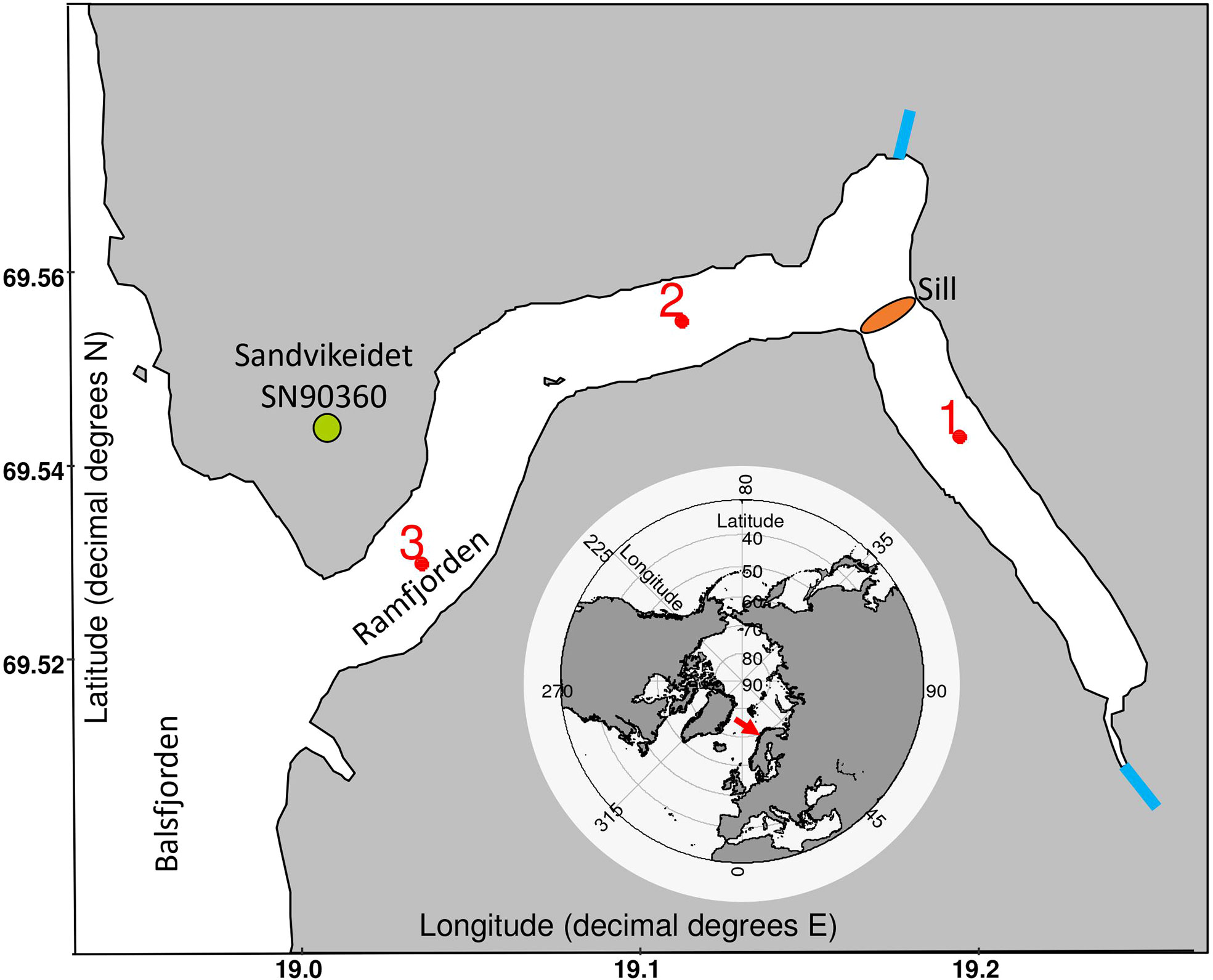
Figure 1 Sampling locations in Ramfjorden. The red numbers and dots show the location of the sampling stations, and the blue lines indicate the two major river inputs. The position of Ramfjorden is indicated by the red arrow on the pan-Arctic map. The shape files were retrieved from www.kartverket.no (2020). The sill in Ramfjorden is indicated by the brown ellipse, the meteorological station at Sandvikeidet as a green circle. The meteorological station in Tromsø is ca 14 km northwest of station 3.

The innermost station (st 1) is typically ice-covered from late winter to spring (late January to May in 2019; see O’Sadnick et al., 2020 for details). During periods of ice cover, water samples were taken through a hole in the ice starting in February. At all stations, water samples were taken at 5 m and 30 m water depth and near the sea floor (ca. 55 m at st1, 110 m at st2, 125 m at st3), using a 5 L Niskin bottle (Seatronics, Åkrehamn Norway). The depths represent three water layers including salinity-stratified surface water (5 m), the depth below the pycnocline but within the euphotic zone (30 m), and bottom water. Due to possible drag of the Niskin bottles we expect an uncertainty in the depth estimation of ±2 m, which is still within the water layer that we aimed to sample. Water samples were collected for determination of phytopigments (Chlorophyll a (Chl), phaeophytin), particulate organic carbon and nitrogen (POC/PON) concentrations and isotopic ratios (δ¹³C, δ¹⁵N), and inorganic nutrients (Phosphate, Nitrate, Nitrite). Samples collected at 5 m and 30 m water depths were analyzed for protist community composition and algal abundances (light microscopy), bacterial abundances (epifluorescence microscopy), molecular microbial (18S and 16S ribosomal RNA (rRNA) sequencing) diversity, and metabolomics profiling (fatty acids, polar compounds). Bacterial and primary production were measured in-situ via isotope probing experiments with ¹³C and ¹⁴C tracer incubations. In addition, vertical phytoplankton net hauls from 35 m to the surface (10 µm mesh size, KC Denmark), CTD casts with irradiance (photosynthetic active radiation: PAR) and Chl fluorescence sensors, and Secchi depth measurements were taken. Due to logistical challenges, not all sampling could be carried out at all depths, stations, or months (Table S1).

2.2 Physical parameters

A CastAway™ (SonTek/Xylem, San Diego, CA, USA) CTD was deployed at all sampling events and a Seabird™ SBE 19plus (Seatronics, Åkrehamnm, Norway) CTD with a planar photosynthetic active radiation (PAR) and a Chl fluorescence sensor from November on. Surface irradiance was measured on land at Olavsvern near station 3 using a Li-Cor planar PAR sensor (Li-Cor Inc., Nebraska, US). Secchi depths (SD, m) were estimated around local solar noon with a weighted white disc. PAR in the water column for September and October were calculated after Esteves (1998) using an SD x k (attenuation coefficient m^-1) value of 1.7 and measured surface PAR levels and Secchi depths. A full-scale meteorological observatory is operated by the Norwegian meteorological office in Tromsø (www.yr.no, station ID: SN90450; variables: temperature, precipitation, snow, wind), ca. 14 km away from Ramfjorden. Air temperatures were also retrieved from a meterological station at Sandvikeidet (station ID: SN90360, temperature), ca. 2 km away from st 3. Additional information about the stations, based on their station ID can be obtained from the Norwegian climate service centre (Norsk Klimaservicecenter, https://seklima.met.no/).

Plus degree days (+dd) were calculated as the number of days with average temperatures above 0°C (at Sandvikeidet) over a period of four weeks prior to the sampling point. We considered +dd as an indicator for potential freshwater runoff and/or snowmelt affecting our individual sampling. We chose four weeks as it represents roughly the time between our sampling events. While freshwater can enter the fjord via direct atmospheric deposition and runoff, we expect terrestrial runoff to be the main source since the fjord area (14 km²) is only about 9% of the total catchment area (159 km², based on topographic maps by kartverket). We used the salinity at 5 m depth as proxy for stratification and freshwater inputs. We also calculated the stratification index based on density differences of the upper 5 m and a maximum depth of 50 m, and pycnocline depths based on the steepest density gradient using the stratif and clined functions of the castr package in R (https://github.com/jiho/castr). +dd and salinity at 5 m were significantly negatively correlated (linear model - lm, p < 2 x10^-16, t=269.6), showing that +dd are indeed a good proxy for potential freshwater runoff from snowmelt. CTD data were interpolated using the mba.surf function of the MBA package in R (Finley et al., 2017) based on the algorithm by Lee et al. (1997). The interpolated data were plotted using the image function of the autoimage package in R (French, 2017).

Time series data for sea surface temperature and salinity were based on remote sensing and modelling products. Temperature data were retrieved via the NAUPLIUS application for the entrance of Ramfjorden at (st.nmfs.noaa.gov/nauplius). Sea surface temperatures (SST) were estimated after the NOAA 1/4° daily optimum interpolation sea surface temperature (OISST) method including data from satellites and in situ measurements since 1982 (Huang et al., 2020). Surface salinity was estimated after the Hadley EN4 subsurface salinity objective analyses and retrieved from Met Office Hadley Centre observations datasets with data since 1950 (Good et al., 2013).

2.3 Biogeochemical variables

Nutrient samples were taken from each depth in triplicates, sterile filtered (0.2 µm pore size Whatmann™ syringe filters, Polyethersulfone membrane) and stored at -20°C until processing. Nitrate and Nitrite were measured on a nutrient autoanalyzer (The San++ continuous Flow Analyser) following protocols by Grasshoff et al. (2009). Orthophosphate was measured manually after Grasshoff et al. (2009). In brief, 2.5 ml of the samples were incubated with 50 μl 2 M H₂SO₄ for about 12 h at 4°C, before adding 200 μl reaction mixture containing 5.2 mmol L^-1 (NH₄)₆Mo₇O₂₄ x4H₂O and 0.5 mmol L^-1 K(SbO)C₄H₄O₆ in 4 M H₂SO₄ (Grasshoff et al., 2009), incubating for 20 min at room temperature and measurement on a spectrophotometer (Hitachi Ratio Beam Spectrophotometer U-1900).

Phytopigment samples (150-300 ml) were filtered onto GF/F filters and stored dark at -20°C until processing. Phytopigments (Chlorophyll a, Phaeophytin a) were measured fluorometrically after Jespersen and Christoffersen (1987). Briefly, phytopigments were extracted in 8 ml 96% Ethanol for about 12 h in the dark at 4°C, before removal of the filter and centrifugation (3000 rpm, 5 min). The remaining extract was measured on a Turner Trilogy AU-10 fluorometer (Turner Designs, 2006) before and after acidification with a drop of 10% HCl. 96% Ethanol was used as a blank and a Chl standard (Sigma S6144) was used for calibration. Fluorescence profiles of the CTD were calibrated with the discrete Chl measurements to obtain a higher vertical resolution and to calculate integrated Chl biomass.

For POC/PON, samples (ca 500ml) were filtered onto pre-weighed precombusted GF/F filters and stored at -20°C until processing. The samples were dried (75°C for ca 12h) and acidified (ca. 12h, in an exicator with HCL fumes), before weighing and measuring on an isotopic ratio mass spectrometer (IRMS) coupled to an Organic Elemental Analyzer (Thermo Scientific FLASH 2000 HT Elemental Analyzer for Isotope Ratio MS) providing both POC/N concentrations and δ¹³C ratios. Those were used to assess the potential influence of terrestrial POC in the fjord system (Kumar et al., 2016).

2.4 Metabolic activities

Primary production was measured in-situ at the Chl maximum at 30 m at the innermost station (st 1) using trace amount additions of ¹³C labelled DIC (Sodiumbicarbonate, Perkin Elmer) (final concentration of addition: 110 µmol L^-1, ca 5% of background concentration) incubations in discrete samples for about 24 h in 10 L carboys (November, December, February). Net primary production was calculated after López-Sandoval et al. (2018), using a reference with identical addition of unlabeled DIC (dark sample in López-Sandoval et al., 2018). We used a mean DIC concentration of 2022+-78 µmol kg^-1 (unpublished data from Ramfjorden by Melissa Chierici, Institute of Marine Research, Tromsø) as estimate for the natural DIC concentration and typical natural δ¹³C DIC values of 0.8‰ (Cheng et al., 2019). Bacterial activities were estimated via ¹³C labelled Glycine (Perkin Elmer) incubations (10 µmol L^-1, ca 10% of estimated dissolved organic carbon background concentration). Either the 1^st (C1, carboxyl group) or 2^nd (C2, organic group) carbon (C) atom was labelled to study the relative role of anabolic and catabolic processes. Anabolic processes (e.g. biosynthesis of proteins or other amino acids), would lead to incorporation of both C groups, while catabolic processes (via NAD+ reduction, Kume et al., 1991) would release the C1 via decarboxylation and lead to incorporation of C2 labeled substrate. The difference between C1 and C2 uptake shows catabolic processes. Controls were incubated with the same amounts of added unlabeled DIC or glycine substrates. Glycine uptake data are given as atomic excess of ¹³C of the labelled vs unlabeled incubations due to a lack of data for natural substrate concentrations and δ¹³C values of Glycine in the fjord. For comparison, we also show atomic excess of ¹³C of the labelled vs unlabeled incubations of the ¹³C-DIC incubations. The samples were filtered onto precombusted GF/F (Whatman) filters and stored at -20°C before drying and acidification as described for POC samples and measurement. The samples were measured on a Thermo Flash EA 1112 elemental analyzer (EA) coupled to an isotopic ratio mass spectrometer (IRMS, Thermo Delta Plus XP, ThermoFisher Scientific, Waltham, MA, USA) as described by Großkopf et al. (2012). Caffeine standards were used for isotope corrections and CN quantification with an accuracy an order of magnitude below the variability between samples.

Between February and April, in-situ primary production was measured via ¹⁴C-DIC (Perkin Elmer) incubations (1 µCi ml^-1) at 5 m (Chl maximum after March) and 30 m (Chl maximum in February) depth below the sea ice. The incubations ran for about 24h in 2-3 light (representing in-situ conditions) and 1 dark bottle (control) incubations with 500 mL seawater per bottle. The samples were filtered onto precombusted GF/F filters and excess DIC removed via HCl acidification in 20 ml Scintillation vials. The incorporated activity was then measured in Ultima Gold™ Scintillation cocktail on a liquid scintillation counter (Perkin Elmer™, Tri-Carb 2900TR) and primary production was calculated after Parsons et al. (1984). Since ¹⁴C-DIC based estimates of primary production are typically 1.3 times lower than ¹³C-DIC based estimated (Regaudie-de-Gioux et al., 2014) we divided the ¹³C-DIC based estimates by 1.3 for comparability.

2.5 Metabolomics

From the in-situ incubations, samples were also filtered onto pre-combusted GF/F filters for metabolomics profiling of fatty acids (FA), and polar compounds (PC, e.g. sugars, amino acids). Lipids were extracted by placing the filters into 3.75 ml CHCL₃:CH₃OH (chloroform and methanol 1:2), and 1 ml PBS (phosphate buffer standard solution). The material on the filter was removed by vortexing and sonication (45 min sonication bath), followed by 15 min vortexing. The filters were then removed, and the remaining material left for extraction at room temperature. After 12 h, 1.25 ml chloroform and 1.25 ml PBS were added and the samples vortexed. The lipid fraction on the bottom of the vials was transferred with a syringe and dried under constant N₂ flow. The upper polar compounds were transferred separately with a pre-combusted glass pipette and dried under a constant N₂ flow and centrifugation under vacuum at 45°C (SpeedVac™, ThermoFisher, Waltham, US). Base saponification of the lipid fraction was achieved via incubation in 2 ml of 6% methanolic KOH for 4 h at 80°C. The samples were diluted in 2 ml of 0.05 mol L^-1 KCl after saponication and neutral lipids extracted after 3 times washing in 2 ml n-Hexane. The remaining fatty acid solution was acidified with 25% HCl to a pH close to 1 and extracted 3 times with 2 ml n-Hexane. The lipids were then dried under a constant N₂ flow and centrifugation under vacuum at 45°C. Before derivatization the extract was dried in a vacuum concentrator for 30 min.

2.5.1 FAME derivatization

Due to the difficulties of detecting free fatty acids on a GC, derivatization to fatty acid methyl esters (FAME) is required (reviewed by Shantha and Napolitano, 1992). Derivatization was performed by adding 1 mL of 14% borontrifluorid (BF3) in methanol onto the dry fatty acid fraction and incubating at 70°C for 1 h. Following the addition of 1 mL of water, the derivatized fatty acids were extracted by three hexane washing (1 mL x 3). The hexane fractions were dried down, the extract resuspended in 100 µL of hexane and transferred to a GC-MS vial for GC-MS data acquisition.

2.5.2 Polar compound derivatization

For polar compounds to be sufficiently volatile for GC analyses, derivatization is necessary (see Orata, 2012). This was performed by adding 80 µL of methoxyamine hydrochloride dissolved in pyridine (20 mg mL^-1) to the extract and incubating the mix at 37°C for 90 min using a thermal rotating incubator under constant rotation at 1350 rpm. Following the addition of 100 µL of N,O-bis(trimethylsilyl)trifluoroacetamide, each extract was vortexed and incubated for another 30 min at 37°C with constant stirring (1350 rpm). The derivatized extract (100 µL) was then transferred to a GC-MS vial for GC-MS data acquisition.

2.5.3 GC-MS data acquisition

The derivatized polar compounds and the FAMEs were analyzed on an Agilent 7890B GC coupled to an Agilent 5977A single quadrupole mass selective detector. An Agilent 7693 autosampler injected 1 µL of sample in spitless mode though a GC inlet liner (ultra-inert, splitless, single taper, glass wool, Agilent) onto a DB-5MS column (30 m x 0.22 mm, film thickness 0.25 µm; including 10 m DuraGuard column, Agilent). Metabolite separation on the column was achieved with an initial oven temperature of 60°C. Then, the temperature was steadily increased (20°C min^-1) until it reached 325°C, when temperature stayed constant for 2 min. Helium was used as a carrier gas at a constant flow rate of 1 mL min^-1. Mass spectra were acquired in electron ionization mode at 70 eV across the mass range of 50 to 600 m z^-1 and a scan rate of 2 scans s^-1. The retention time was locked using standard mixture of fatty acid methyl esters (Sigma Aldrich).

2.5.4 Data analyses

Raw GC-MS data were imported into R as converted mzXML files (msConvert) and processed using XCMS. Individual peaks were picked using the CentWave algorithm with the default parameter recommended for GCMS data by XCMSonline. Resulting peaks were grouped, retention times corrected and regrouped using the density (bandwidth parameter set to 2) and obiwarp methods. Following peak filling, the CAMERA package was used to place m/z peaks into pseudo-spectra by grouping similar peaks with the groupFWHM function. Samples with a low internal standard signal (<5e4) were excluded from the analysis.

A single m/z value was selected to represent each CAMERA group using the following criteria: 1) m/z value > 150, 2) occurs across samples with the highest frequency and, if two or more ions are tied in terms of number of samples detected, 3) has the highest mean intensity. Ions with very low mean intensities (< 0.001) were considered noise and removed from the analysis.

Following data processing, the resulting ion abundances from individual peaks were normalized to the ribitol internal standard. Multivariate analyses were done in R using the vegan package. The NMDS plots are based on Bray-Curtis dissimilarities. The script used for the analysis is available on github (https://github.com/Tobivnnhm/Ramfjord_Polar_night).

2.6 Communities and biomass

Phytoplankton net and/or water samples were fixed in 2% neutral Lugol and stored in brown borosilicate bottles in the dark. The samples were investigated via light microscopy using the Utermöhl (1958) method (50 ml settling chambers, for 24 h) for quantitative estimates (water samples), or in 2 ml well plates for qualitative estimates (phytoplankton net). Protists were counted and identified under an inverted light microscope (Zeiss Primovert, Carl Zeiss AG, Germany) under 10x40 magnification. Taxa were identified using identification literature by Hasle et al. (1996), Tomas (1997) and Throndsen et al. (2007). Due to generally low cell numbers in the polar night, taxa were pooled into higher taxonomic levels to assure at least 15 counts per group per sample.

DNA samples were filtered immediately after sampling onto sterivex™ filters using a peristaltic pump for 30 minutes (2-5L). Filters were stored at -20°C until extraction. The filter was cut out from the cartridge using sterile scalpels and DNA was extracted using the DNeasy^® PowerSoil^® kit with some modifications, described by Vonnahme et al. (2021b). For bacterial community composition analysis, the V4 region of a ca. 292 bp fragment of the 16S rRNA gene using the primers (515F, GTGCCAGCMGCCGCGGTAA and 806R, GGACTACHVGGGTWTCTAAT, assessed by Parada et al., 2016) was amplified. For eukaryotic communities the v7 region of the 18S rRNA gene (100-110 bp inserts) was amplified using the primers (Forward 5’-TTTGTCTGSTTAATTSCG-3’ and Reverse 5’-GCAATAACAGGTCTGTG-3’, Guardiola et al., 2015). The Illumina MiSeq paired-end library was prepared after Wangensteen et al. (2018).

Bacteria were counted after DAPI (4,6-diamidino-2-phenylindole) staining as described by Porter and Feig (1980). 25 ml of the water sample was fixed in 2% formaldehyde for at least 12 h and filtered onto 0.2 µm pore size polycarbonate filters and washed with sterile filtered seawater and 96% ethanol before drying. The filter were then incubated in 30 µl DAPI (1 µg ml^-1) for 5 min in the dark before washing with MQ and 96% ethanol and embedding in Citifluor™:Vectashield™ (4:1) onto a microscopic slide. Bacteria were counted under UV light at 10x100 magnification in at least 10 grids or 200 cells, using an epifluorescence microscope (Leica DM LB2, Leica Microsystems, Germany).

2.7 Bioinformatics and statistics

Amplicon sequences were analyzed using a pipeline modified after Atienza et al. (2020) based on OBITools v1.01.22 (Boyer et al., 2016). The raw reads were demultiplexed and trimmed to a median phred quality score minimum of 40 and sequence lengths between 215 bp and 299 bp for 16S amplicons and between 80 bp and 190 bp for 18S amplicons and merged. Chimaeras were removed using uchime with a minimum score of 0.9. The remaining merged sequences were clustered using swarm (Mahé et al., 2014). 16S swarms were classified using the RDP classifier (Wang et al., 2007). 18S swarms were classified using the silva database as described by Atienza et al. (2020). Multivariate analyses were done in R using the vegan package. The NMDS plots were based on Bray-Curtis dissimilarities. The main drivers of changes in protist communities were identified using the adonis function (permutational multivariate analysis of variance based on Bray-Curtis dissimilarity matrices), using sample type, month, and station as explanatory variables. To consider mixed effects, sample type and month constrained the permutations via the strata argument. The different stations were assumed to be similar to each other and not included in the strata argument. Correlation analyses between paired samples were done in R using Pearson’s product moment correlation coefficient. The hypothesis of surface temperature, stratification and light as main drivers of the biogeochemical properties was tested via redundancy analyses (rda function of the vegan packagae in R) followed by an ANOVA (aov function in R). PAR, +dd and Salinity at 5 m depth were the explanatory variables and the biogeochemical data (Nutrients, Chl, Phaeophytin, PN, POC, C:N, δ¹³C-POC, δ¹⁵N-PN) were the explained variables. We did not rarefy the dataset as we only studied Bray-Curtis based dissimilarity structures where the most abundant taxa play the largest role (Roden et al., 2018).

3 Results

3.1 Physical environment

Air temperatures (Figure 2A) at Sandvikeidet and Tromsø decreased from October to February. They started to be below 0°C in November and stayed mostly below 0°C in the period December to March (-17.6°C to 8.7°C). Short melting events occurred in January and February. Interestingly, air temperatures near Ramfjorden at Sandvikeidet were generally lower than in Tromsø. Precipitation lacked a clear seasonal pattern throughout the sampling period. Low precipitation as rain occurred from October to the beginning of November. Snow accumulated at a higher rate from the end of December, leading to the accumulation of an over 1 m thick snow cover on the sea ice by April. Wind speed showed no clear seasonal pattern over the sampling period but had strong variations with frequent stronger wind events above 6 m s^-1 average and 8 m s^-1 maximum. The average daily surface irradiance showed strong seasonal variations with PAR values below 1 µE m^-2 s^-1 at the surface and in the ocean below 1 µE m^-2 s^-1 from the end of November to mid-January, with increases starting in February after the end of the polar night (Figure 2D).

FIGURE 2

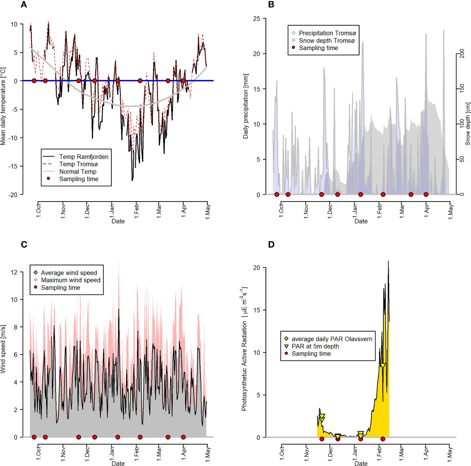
Figure 2 Meteorological data in Tromsø and Ramfjorden. Sampling events are marked with a red circle. (A) Daily average temperatures in Tromsø (red line) and Sandvikeidet/Ramfjord (black line) in relation to average temperatures averaged over the past decades (grey line). (B) Daily average (blue area) precipitation and snow depth (greay area) for Tromsø. (C) Daily average (grey area) and daily maximum (red area) wind speeds for Tromsø. (D) Irradiance data (PAR) measured at Olavsvern north of st3 (daily average as yellow area), and at 5 m depth during the sampling (yellow triangles).

CTD profiles (Figure 3) revealed a strongly salinity-stratified water column at all three stations from end of September to October (Stratification index = 0.9 - 2.7 kg m^-3) with pycnoclines below 3.1 m depths coinciding with air temperatures above 0°C. Later, temperatures fell below 0°C leading to a mixed water column (pycnocline below 33 m) and increasing surface salinity (Stratification index = 0.2 - 0.5 kg m^-3, Table S2). At station 1 and 3 the water column re-stratified briefly in January (Pycnocline at 0.9 - 2.5 m, Table S2) following heavy precipitation, strong wind, and a melting event (Figures 2A-C). Ocean temperature exhibited weak vertical gradients, but a seasonal decrease (Figures 3D-F; Table S2). The remote sensing data revealed significantly increasing sea surface temperatures over the time period 1982 to 2020 (Seasonally Adjusted Mann Kendall test, tau=0.096, p<0.00) (Figure S2A) but no trend in surface salinity for 1950 to 2020 (Seasonally Adjusted Mann Kendall test, tau= -0.037, p<0.11) (Figure S2B).

FIGURE 3

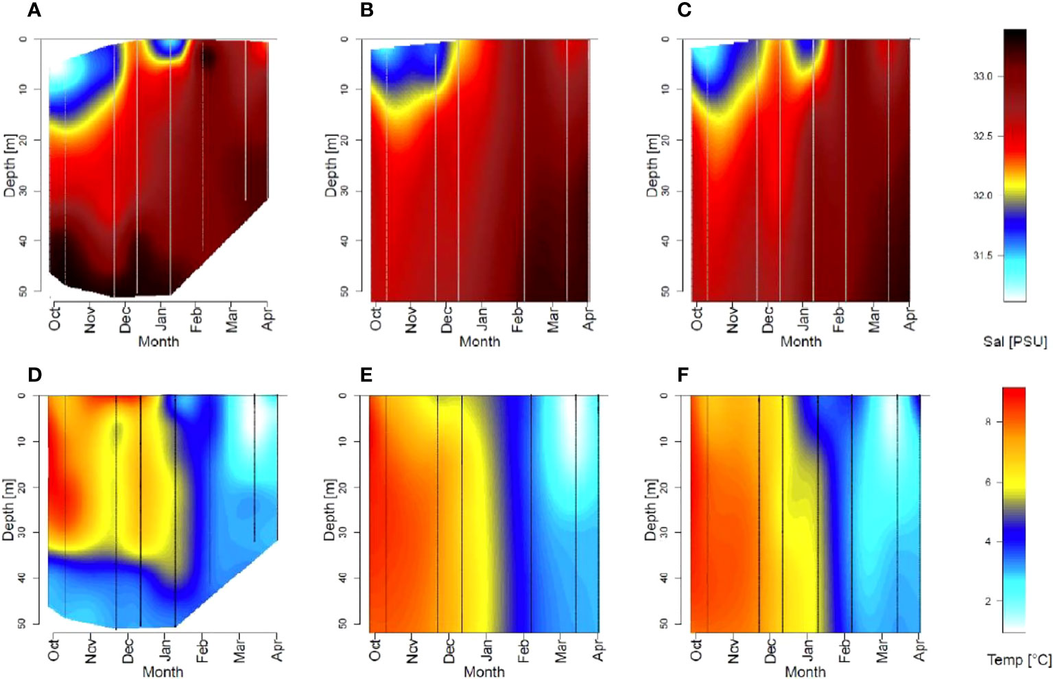
Figure 3 Seasonal changes of salinity (> 31 PSU, A–C) and temperature (D–F) in Ramfjorden for stations 1 (A, D), 2 (B, E) and 3 (C, F) for the upper 50m of the water column. Vertical lines indicate the time and depth of measurements.

3.2 Biogeochemistry

Nutrient concentrations of phosphate, nitrate, nitrite, and ammonium showed similar changes over time (Figures 4, S1). We focused on NO_X (nitrate + nitrite) concentrations as key nutrient (Figures 4A, D), as it is typically limiting in the Arctic, for phytoplankton productivity. In September and October NO_X concentrations were lowest (< 0.5 µmol L^-1) at the surface and slightly higher at 30m depth. While C:N ratios were consistently above Redfield (6.6) they were relatively low (approx. 15 at 5m depth) at this time. δ¹³C-POC were higher compared to the polar night values. In November, coinciding with the vertical mixing of the water column, NO_X concentrations increased to about 4 µmol L^-1, while C:N ratios at 5 m increased to about 25 and δ¹³C-POC values decreased slightly at 5 m but increased at 30 m depth. NO_X concentrations and C:N ratios stayed high until March, when NO_X concentrations and C:N ratios dropped at 5 m depth. The decreasing C:N ratios in April corresponded to strongly increasing Chl concentrations (Figures 4, 5). δ¹³C-POC values already started increasing in February, when PAR at 5 m reached values above 1 µE m^-2 s^-1, while Chl concentrations were still low and air temperatures below 0°C.

FIGURE 4

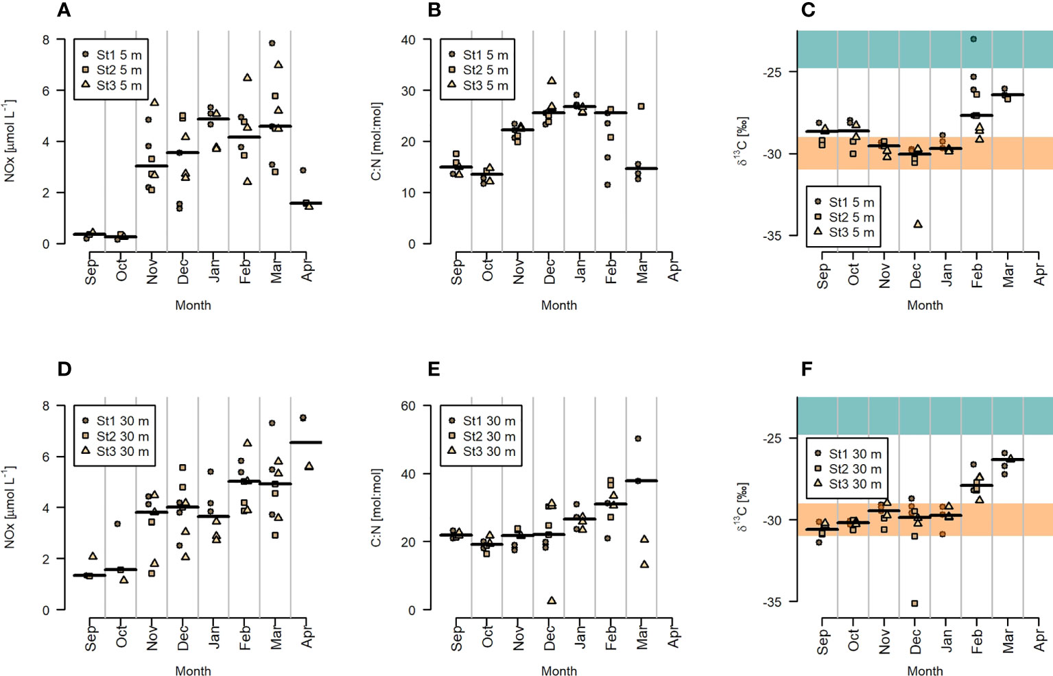
Figure 4 Biogeochemical indicators with dissolved inorganic NO_X (A, D) and molar C:N ratios (B, E) as proxies for the nutritional state and δ¹³C-POC (C, F) as proxy for the origin of organic particulate matter. Plots (A–C) show data for 5 m depth and plots (D–F) data for 30 m depth. Horizontal black lines show the median of all data of the month, and different symbols indicate the individual data for the three stations. Terrestrial δ¹³C-POC values reported by Simenstad and Wissmar (1985) are marked in orange, coastal phytoplankton δ¹³C-POC values reported by Simenstad and Wissmar (1985) are marked in green.

FIGURE 5

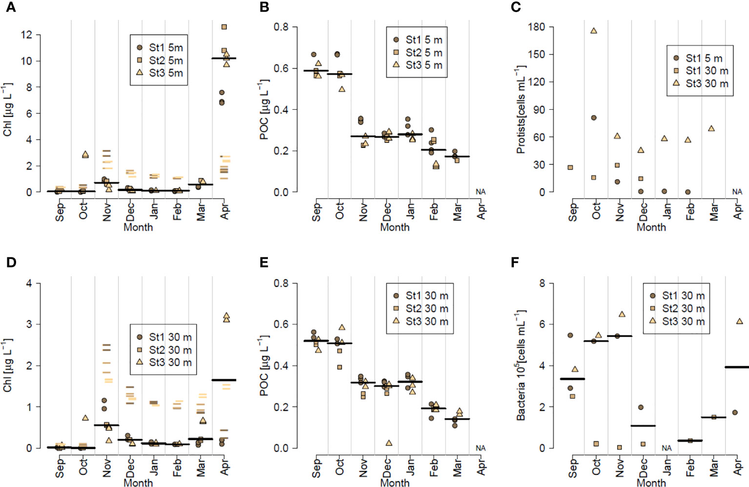
Figure 5 Biomass indicators for phytoplankton (Chlorophyll a (Chl); A, D and Phaeophytin a, as -), particulate organic matter (POC; B, E), bacteria (abundance, F), and protists abundance (C). Plots a-b show data at 5 m depth. Plot C data at 5 m and 30 m depth, and plots (D–F) data at 30 m depth. Note the different scales used for a and d. Horizontal black lines represent the median of all data (excluding Phaeophytin a) of the month, and different symbols show the individual data for the three stations. Missing data for April are marked with NA.

Chl concentrations (Figure 5) slightly increased from low September and October values (median at 5 m= 0.05 µg L^-1) to higher November concentrations at 5 m and 30 m depths (median = 0.7 and 0.6 µg L^-1). This was strongest at station 1, with the shallowest water depth and strongest connection to land. Chl concentrations stayed low after November, until concentrations started increasing in March. A very high peak occurred in April (median at 5 m=10.2 µg L^-1), with higher and deeper reaching concentrations in the outermost ice-free stations (st2, st3). Phaeophytin concentrations followed the Chl trend but were about 5 – 10 times higher than Chl during the polar night (Nov-Mar) and lower or equal to Chl during autumn and spring. POC values were decreasing from October to lowest values in March (median=0.15 µg L^-1) – no measurements were available for April for the phytoplankton bloom. Protist abundances were consistently highest at station 3, with a maximum in October (1.75x 10⁵ cells L^-1 at 30 m, 8.1 x 10⁴ cells L^-1 at 5 m) – no data were available for April. The seasonal changes in the bacterial abundances generally corresponded to POC and/or Chl concentration changes with lowest values during the polar night period (December-February) and highest values in November and April.

3.3 Physical drivers of biogeochemical changes

Multivariate redundancy analyses (Figure 6) revealed that potential freshwater runoff (+dd), potential stratification (salinity at 5 m) and PAR significantly (p=0.002, F=3.15, ANOVA) explained 49% of the variation of biogeochemical variables at 5 m depth with Salinity and +dd as the most important explanatory variables (approx. 36% combined). As described above, October was characterized by high light, high potential runoff and high stratification. Irradiances decreased towards the polar night and increased towards March (Figure S3 and Table S2). Decreasing potential surface runoff and stratification were observed until April, when the proxies for both drivers reversed. High potential runoff was related to high particulate organic matter (POM) and nitrite concentrations, while low runoff was related to higher phosphate and nitrate concentrations. High light levels were related to high δ¹³C ratios and low Phaeophytin concentrations. Chl was only weakly related to a less stratified water column and higher irradiance levels.

FIGURE 6

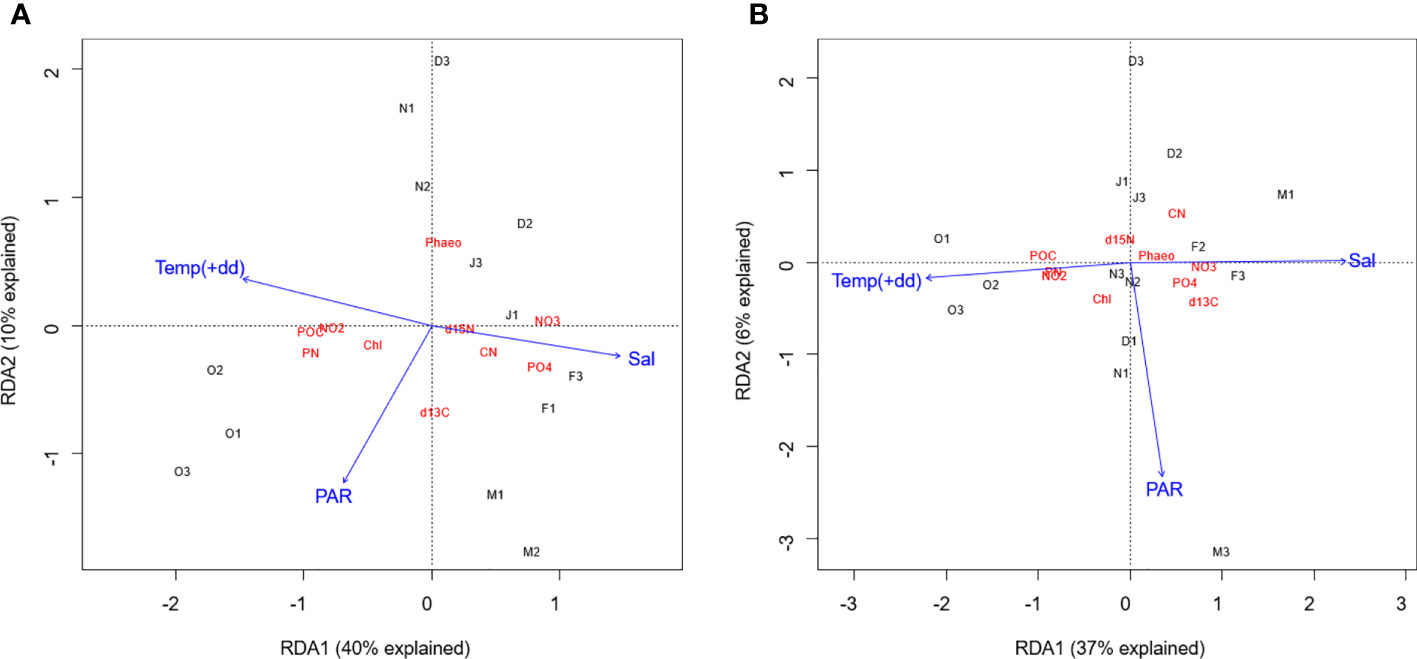
Figure 6 Redundancy analyses at (A) 5 m depth and (B) 30 m depth (RDA function in the vegan package in R) with three main physical drivers (blue). With PAR as proxy for light availability, Temperature in +-degree-days (days with mean air temperatures above 0°C, 4 weeks before the sampling) as proxy for potential freshwater runoff, and Salinity at 5 m depth as proxy for stratification (Based on the assumption that salinity being the main driver of density variability). Explained variables (red) were the z-standardized (sd=1, mean=0) biogeochemical parameters. Samples (black) are indicated by the first letter of their sampling month and station number.

3.4 Metabolic activities

Activity measurements were available starting November at 30 m depth and starting February also for 5 m depth using ¹³C and ¹⁴C DIC tracer incubations (Figure 7). Net primary productivity (NPP, ¹³C incorporation) was detectable at very low levels throughout the polar night (<0.08 mgC m^-3 d^-1, November-February). In March, NPP increased at 5 m and reached a peak of 1.6-4.1 mgC m^-3 d^-1 in April. Glycine incorporation had a maximum in November for both C1-glycine (carboxyl group) and C2-glycine (organic group) incorporation with little difference between C1 and C2 (mostly anabolic uptake). In December, the organic C2 group of glycine was taken up preferably with almost no incorporation of the labeled C1 carboxyl group (mostly catabolic processes). In February, both the organic and carboxyl C groups of glycine were incorporated into biomass with a slightly higher uptake of C1 (anabolic process and cross-feeding; CO₂ cleavage and uptake by phototrophs). Consequently, the carboxyl C1 group labeled glycine was only taken up when light was present.

FIGURE 7

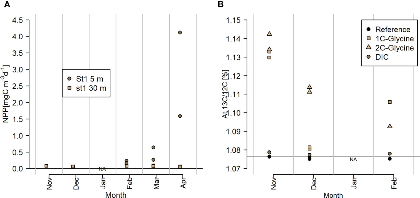
Figure 7 (A) Net primary productivity estimates based on isotope enrichment experiments after 24 h in situ incubations with ¹³C-DIC (30m Nov-Feb) and ¹⁴C-DIC (rest), (B) Atomic 13C/12C ratio (%) as proxy for uptake of ¹³C₁-glycine (carboxyl C group), ¹³C₂-glycine (organic C group) and ¹³C-DIC (Nov to Feb only).

3.5 Bacterial and Archaeal communities

The dominant bacteria and archaea taxa were very similar throughout the study period (Figure 8). While October and November communities appeared slightly separated from the rest based on the NMDS plot, a low stress value on OTU level is indicative of very low variability between samples. The most dominant classes had very similar community structures over the sampling period with Alphaprotoebacteria (24-32% SAR11 clade, Pelagibacter) and Gammaproteobacteria (Methylosphaera 23-32%) contributing about 50% to the 16S based communities. The nitrifying archaeal group Nitrosopumilales was the most abundant archaea group throughout the study period. However, seasonal patterns appeared for some less abundant bacteria and archaea classes. Flavobacteria, Actinobacteria, and Planctomycetia were relatively abundant groups with seasonal changes in their community structures. Flavobacteria were dominated by Aquibacter in October (57%), which gradually decreased until April, while Owenweeksia appeared as dominant taxa in February (29%) with a following decrease. Actinobacteria were dominated by Euzebyaceae in October (69%), which got gradually replaced by Acidimicrobineae towards April (47%). Deltaproteobacteria and Thermoplasmata were also abundant classes. 99.9% of Thermoplasmata were related to Methanomassiliicoccales. Deltaproteobacteria showed a distinct seasonal pattern of Deferrisoma spp. being dominant in October (37%) and gradually decreasing towards April, Labilitrichaceae being most dominant during the polar night (11-13%) and Desulfatitalea becoming gradually more abundant towards April (38%).

FIGURE 8

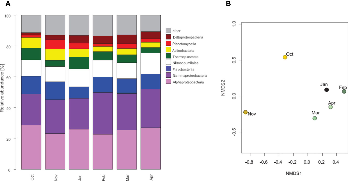
Figure 8 Bacterial and archaea community structures. (A) Most abundant classes of bacteria and archaea (3 most abundant classes in at least 1 month) at 30 m depth at station 1. (B) NMDS plot of the communities (stress = 0).

3.6 Protist community composition

Protist communities were significantly varying with time (Permutational Multivariate Analysis of Variance: adonis, p=0.001) but were similar in their dominant groups of diatoms (Bacillariophyceae and Coscinodiscophyceae) and dinophytes (Dinophyceae; Figures S4, 9). Diatoms were most dominant in autumn (October-November) communities, while the polar night (December-February) communities were dominated by Dinophyceae and other flagellates.

FIGURE 9

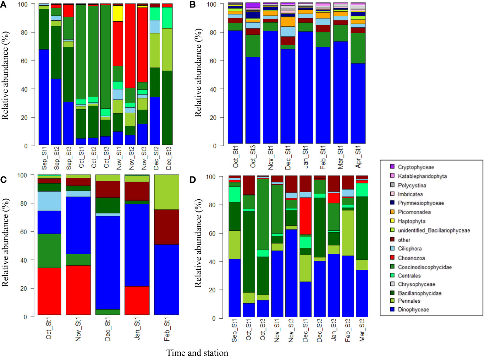
Figure 9 Protist community structures. Most abundant taxa (primarily in classes) in (A) phytoplankton net samples (Net), (B) 18S sequencing samples, (C) water samples at 5 m, and (D) water samples at 30 m. The sample origins are indicated at the bottom label. Months are indicated by the first three letters of their names.

The community structures were also highly variable between different sampling methods (18S sequencing, phytoplankton net, water samples, adonis, p=0.001). In particular, dinoflagellates were significantly more abundant based on the18S sequences compared to the microscopy counts. In addition to method, water depth was another important explanatory factor with the largest variation during the autumn bloom (October/November, Figure S4b). The polar night communities were generally more similar between the different depths.

An autumn algal bloom, as indicated by high abundances, was most pronounced at st 3 in October (Figure 4). The October bloom at st 3 was dominated by Skeletonema sp. followed by Pseudo-nitzschia sp. and ciliates in the phytoplankton net hauls. 18S sequences showed a similar structure, but higher contributions of dinoflagellates and lower contributions of Pseudo-nitzschia sp. Light microscopy revealed a large number of dinoflagellate resting spores within the autumn community (1.28 x 10³ spores L^-1, 18.6% of total dinoflagellates). At the other stations an even later bloom occurred at 30 m in November (Figure 4). Pseudo-nitzschia sp. and choanoflagellates became more abundant in the surface layer whereas the contribution of Skeletonema sp. decreased. In the deep (30 m) Chl maximum, Skeletonema sp. was still abundant, but dinoflagellates became dominant, contributing up to 75% to the microscopy-based protist communities of the water samples.

During the polar night, protist abundances dropped to a minimum of 4.1 x 10² cells L^-1 in February in water samples. As the polar night progressed, dinoflagellates were concentrated further up in the water column and gradually increased their relative contribution in the surface layer (5 m) from 25% in November to 71% in February. Besides Dinophyceae, choanoflagellates and pennate diatoms were most abundant during the polar night. 18S sequences provided further details about the protist taxonomic diversity during the polar night. The dominating polar night dinoflagellate taxa were Prorocentrum minimum, Amoebophrya sp., Gyrodinium helveticum and other Gyrodinium sp, Stramenopiles sp., and Karlodinium veneficum. Gymnodiniaceae were most abundant from October to January and the relative contribution decreased when the light returned in February. In addition the picomonad Picomonas judraskeda and Stramenopiles occurred frequently. The most abundant diatoms during the polar night were Skeletonema sp., Chaetoceros sp. and Pseudo-Nitzschia sp. The parasitic dinoflagellate genus Amoebophryra spp. was present throughout the study period. Amoebophrya spp. were positively correlated to Gyrodinium spp. (R² = 0.78), Gymnodinium spp. (R² = 0.59), Karlodinium spp. (R² = 0.47), and Prorocentrum spp. (R² = 0.44). Other dominant taxa identified during the polar night were other heterotrophic protists, such as Polycystina. Chaetoceros gelidus became the most dominant species in the following April spring bloom as evident from 18S sequences and the phytoplankton net data.

3.7 Metabolomics

Metabolomics (polar compounds (PC) and fatty (FA) acid composition of POM) analyses of st 1 at 30 m revealed two to three potential temporal clusters (Figure S5). PC profiles revealed three potential temporal clusters of 1) September and November, and 2) October, December, and 3) January. January metabolomics composition was most different compared to any other month which was not the case for the biogeochemical data. FA profiles were generally more homogenous and revealed two clusters separating 1) the polar night (December, January, February) from 2) autumn samples (September, October, November).

4 Discussion

4.1 Seasonal drivers of protist diversity, production, and biomass

4.1.1 Initiation of the spring phytoplankton bloom

According to our first hypothesis, incident solar radiation is the main driver of the initiation of the spring bloom. Already in 1976 and 1978, Eilertsen and Taasen (1984) identified incident solar radiation as the main cause for allowing for a March phytoplankton spring bloom in Balsfjorden (fjord that branches into Ramfjorden) in a fully mixed water column. In both studies polar night conditions limited algal growth until the end February and a spring bloom starting in March was evidenced by increasing NPP, increasing Chl, and high cell numbers of bloom forming diatom species dominated by the chain-forming diatom Chaetoceros gelidus (formally named C. socialis) with reaching its peak in April. However, Fragilariopsis oceanica, which was dominant in the 1970s was rather rare in 2019 potentially caused by regional differences between Balsfjorden and Ramfjorden, interannual variabilities, or a changing climate.

Our 18S metabarcoding allowed a more analysis of protist community changes compared to the 1970s. Based on metabarcoding the protist community structure already shifted to more phototrophic diatoms and less heterotrophic protists in February at very low light levels (< 10 μE m^-2 s^-1 at 5 m), which was not detectible in the microscopic data from neither the 2019 nor the 1970s Thus, we suggest a combined molecular and microscopic approach to detect novel spring bloom dynamics. This would allow to identify trends and changes in biological properties and relate those with environmental drivers in long term time series.

Although barcoding indicated increased photosynthetic activity in February, algal biomass remained low in March, which we attribute to a combination of vertical export rate and a high mixing exceeding euphotic layer production until April (critical turbulence hypothesis, Huisman et al., 1999). At this time, the net heat loss to the atmosphere with limited freshwater input caused deep convection, and algal production remained rather low. In April the reversed heat flux allowed the build-up of algal biomass in a less intensively but still fully mixed column (Huisman et al., 1999; Hegseth et al., 2019). The low zooplankton biomass during this time (Coguiec et al., 2021) indicates a minor control of algal growth by grazing. Therefore, we suggest that spring bloom dynamics was mainly explained by the critical turbulence hypothesis and not the dilution-recoupling hypothesis (Behrenfeld, 2010). Nevertheless incident solar radiation (our 3^rd hypothesis) was a key driver of spring production.

The presence of a seasonal fast ice cover is an additional factor delaying the spring bloom formation at st1 due to its high albedo and light attenuation. While sea ice algae blooms can play an additional role in stimulating phytoplankton algal growth after ice melt, only very low sea ice algae biomass was observed in Ramfjorden mainly due to limited brine volume fractions (Persson, 2020). In April, the light reduction by the sea ice cover likely limited algal growth to only the surface layer (5m) at st1, while the ice free st 3 experienced already a deep Chl maximum and surface NO_X depletion with C. gelidus dominating at both sites. Potentially, the high biomass at st 1 could have been advected from st 3 as suggested earlier (Eilertsen and Taasen, 1984). Light limitation also explains why the NPP at st 1 under the ice was orders of magnitude lower (peak of 1.6-4.1 mgC m^-3 d^-1 in April at 5 m) than data from in the ice-free Balsfjorden in the 1970s (ca 120 mgC m^-3 d^-1 in April at 5 m).

Sea surface temperature and salinity had changed little in Ramfjorden since the 1970s. However, sea surface temperature is projected to increase and sea surface salinity to decrease in the future (IPCC, 2022), and the resulting earlier water column stabilization may supporting earlier onset of the spring bloom based on the critical depth hypothesis (Sverdrup, 1953). However, our results do indicate currently a phenology control by vertical mixing, therefore potentially limiting climate change effects due to temperature and salinity. Increased river runoff could cause increased brownification (brown DOM) and sediment inputs in coastal areas (Aksnes et al., 2009; Opdal et al., 2019), delaying algal bloom formation by reducing light availability (Opdal et al., 2019). The differences between st 1 and st 3 indicate that future loss or earlier melt of sea ice could lead to earlier phytoplankton blooms and higher NPP in currently ice-covered fjords, similar to high Arctic observations (Ardyna and Arrigo, 2020). Detecting such changes on bloom timing and community composition will require continuous long-term time series.

4.1.2 Grazing and mixing are key drivers for the autumn phytoplankton bloom

Our second hypothesis suggested that strong vertical mixing can initiate an autumn phytoplankton bloom through both nutrient upwelling and dilution of grazers. Irradiance did not control autumn bloom formation, as Chl concentrations in September were as low as during the polar night. Also our redundancy analyses showed that potential freshwater runoff (+dd) and stratification (salinity at 5 m) are more important drivers for biogeochemical variables than light in autumn.

Indications for an autumn bloom after September are the occurrences of deep Chl maxima and high diatom abundances in November. We suggest that a deep mixing event in October/November had caused upwelling of nutrients into the surface layers, which we missed due to our course temporal resolution. The cold-water masses at st 1 from depth up to 5 m could also have been created by that upwelling event. While upwelling can cause resuspension of bottom sediments and associated algae (specifically at the relative shallow site st1), the high number of intact diatom cells (cells with chloroplasts) suggests an earlier bloom as the more likely source.

The change in algal biomass during a bloom always depends on the balance between growth and loss terms. During algal spring blooms, zooplankton (meso- and microzooplankton) grazing can suppress phytoplankton biomass accumulation even when primary production is high (Sherr et al., 2009; Behrenfeld, 2010). This general observation was used to develop the dilution–recoupling hypothesis that states that deep mixing and dilution of zooplankton and thereby grazing pressure is at times more important for control of phytoplankton biomass accumulation than a favorable light climate in a stratified water column (Sverdrup, 1953; Behrenfeld, 2010; Saiz et al., 2013). To our knowledge, this hypothesis has not yet been applied to autumn conditions for sub-Arctic fjords, where nutrient resupply via deep mixing is usually considered to be the key driver (Eilertsen and Taasen, 1984; Wihsgott et al., 2019). We argue that this hypothesis also needs to be considered for autumn studies. A recent study in Ramfjorden found high abundances of herbivorous/omnivorous zooplankton (> 4 x 10⁵ individuals m^-2; mostly Oithona similis and Pseudocalanus spp.) from September to November, with zooplankton abundances and biomass in November even exceeding those during the rest of the year (Coguiec et al., 2021). In addition, microzooplankton grazers can consume a large fraction of primary production in a range of Arctic and sub-Arctic fjords (e.g., Verity and Vernet, 1992; Yang et al., 2015). While we did not measure grazing rates directly, smaller microzooplankton was highly abundant in our study (choanoflagellates, dinoflagellates, ciliates) exceeding the abundances of diatoms in November (1.4 x 10⁴ cells L^-1 at 30 m). These observations show that, in autumn, grazing by micro- and mesozooplankton may indeed be a key control of phytoplankton biomass accumulation. However, during this period nutrient concentrations were low. To fully identify the relative importance of grazing pressure and nutrient limitation, direct and combined measurements of primary production as well as grazing activities by zooplankton are needed. The earlier study by Eilertsen and Taasen (1984) found an apparent lack of correlation between algae biomass and nutrients in autumn, indicating that grazing pressure may be a more important driver than nutrients. After restratification, the phytoplankton biomass in the stratified surface layer declined and settled out to deeper depths (including 30 m) likely due to a combination of nutrient depletion and increased grazing pressure. Eventually, the bloom terminates due to the onset of the polar night in November.

Future studies are needed to detect these short-lived mixing event-driven autumn blooms via more frequent sampling, remote sensing or event-based sampling in response to meteorological changes. Considering the increasing temperatures and precipitation with climate change (IPCC, 2022) these weather windows allowing mixing and causing autumn blooms may be delayed potentially into periods when light limitation could cause a loss of autumn blooms in high latitudes. However, in a seasonal ice zone like the inner parts of Ramfjorden, delayed formation or absence of sea ice may lead to increased wind mixing and prolonged light availability in autumn, which may facilitate autumn blooms in these areas (Ardyna and Arrigo, 2020).

4.1.3 Light limitation and survival strategies for phototrophs during the polar night

Due to the absence of light, the polar night has long been considered as a biologically inactive season. However, recently more attention was given to biological processes at low light intensities, revealing that even low irradiance (PAR values of 0.5 μE m^-2 s^-1) is sufficient for photosynthesis of low-light adapted Arctic microalgae during the polar night (Berge et al., 2015a; Berge et al., 2015b; Kvernvik et al., 2018; Johnsen et al., 2020). Hence, we selected 0.5 μE m^-2 s^-1 irradiance at 5 m depth as a threshold under which we assumed photosynthetic growth to be absent. The PAR values at 5 m water depth were only slightly lower than surface PAR values due to the low concentrations of light-absorbing organic particles (POC, Chl) in the water column. Thus, we used the continuous record of surface PAR data to define polar night conditions and discuss light limitation for phytoplankton. Accordingly, true Polar Night conditions at our sampling site lasted from late November to late January. During this time, algal biomass and abundances were low (Chl, relative 18S based abundance, cell counts), Phaeophytin to Chl ratios were high, and δ¹³C-POC values low. NPP was measurable due to the large incubation volume (0.5 L) and long incubation time (24h) but had been very low (0.01 mgC m^-3 d^-1).

The decreasing δ¹³C-POC values during the polar night can be related to decreasing marine primary production or increasing relative importance of terrestrial C (autochthonous C source, Simenstad and Wissmar, 1985). Polar night δ¹³C-POC values at 5 m around -29.5‰ (IQ=-29.7‰ to -29.3‰) were in fact close to values of terrestrial POC (range of -29‰ to -31‰; Simenstad and Wissmar, 1985), while the autumn bloom values around -28.1‰ (IQ=-28.1‰ to -28.0‰) and spring values around -26.1‰ (IQ=-26.4‰ to -25.7‰) are more similar to coastal phytoplankton values (-22.7‰ ± (sd) 2.1‰; Simenstad and Wissmar, 1985). However, the autumn values are very close to the polar night values with only 1‰ difference. For the spring bloom, a combination of increased marine NPP and decreased river runoff contributes likely both to the increasing δ¹³C-POC.

Irradiance was clearly limiting photosynthesis during the polar night. However, algae have developed a multitude of strategies for growth and/or survival under these conditions including parasitism, mixotrophy, reduced activity, dormancy or spore formation, usage of storage compounds, (Zhang et al., 1998; Cleary and Durbin, 2016; Johnsen et al., 2020). Overall, the polar night protist community became more dominated by heterotrophic, or mixotrophic taxa, including their parasites. The dominance of known mixotrophic dinoflagellates during the dark period of our study indicates that mixotrophy is an important survival strategy. With the dominance of dinoflagellates, also their parasites, namely the parasitic dinoflagellate Amoebophyra spp. became abundant and diverse (238 OTUs) with a wide range of potential hosts (Dinophysis, Alexandrium, Gonyaulix, Karlodinium, Prorocentrum, and Scripsiella). Also typical heterotrophic phagotrophic protists (e.g. Monier et al., 2013) such as choanoflagellates, Polycystina, and ciliates became relatively more dominant during the polar night. High latitude phytoplankton may also survive using intracellular storage compounds such as carbohydrates and lipids (Zhang et al., 1998).

Temperature with reduced metabolic rates is a crucial factor determining the length of dark-survival (Smayda and Mitchell-Innes, 1974). The common genus Skeletonema has previously been described as the only diatom taxon to thrive during the polar night in our study area (Eilertsen and Degerlund, 2010). Skeletonema sp. can survive up to 24 weeks of darkness at 2°C, which is well beyond the polar night period of our study (Smayda and Mitchell-Innes, 1974). Efficient dark inorganic nitrogen uptake is one proposed mechanism for their dark survival (Stenow et al., 2020). At higher temperatures, heterotrophic activities increase, and the survival period decreases (Smayda and Mitchell-Innes, 1974), indicating their vulnerability to a warming climate.

4.2 Seasonal drivers of bacteria and archaea communities, activities, and biomass

4.2.1 Allochthonous vs autochthonous C sources for prokaryotes in autumn/winter

While growth of phytoplankton is primarily controlled by light, nutrient availability, and grazing, heterotrophic prokaryotes are dependent on organic matter (OM) as carbon source. In coastal areas, OM may originate from marine primary production or terrestrial inputs (Figueroa et al., 2016). Especially in systems with low primary production (such as the polar night), allochthonous DOM may be the main C source for bacterial growth (Figueroa et al., 2016). Yet, the importance of allochthonous carbon for bacteria in coastal Arctic systems has only recently been considered (Sipler et al., 2017a; Sipler et al., 2017b; Delpech et al., 2021). According to our 3^rd hypothesis allochthonous organic matter inputs from land can feed an active polar night microbial community.

We found overall evidence of both locally produced and allochthonous carbon sources being important for bacteria biomass but having only limited effects on prokaryotic community structures. In September/early October bacteria abundances were high despite low Chl concentrations and high abundances of potential bacterivorous organisms (e.g. microzooplankton, choanoflagellates). High amount of freshwater inputs (salinity-stratified surface) potentially provided terrestrial OM as main carbon source during this time as also evidenced by low δ¹³C-POC, high δ¹⁵N-PON, and high POC/Chl ratios.

While our proxies for surface runoff (surface salinity, +dd) and terrestrial OM inputs have their limitations, we argue that they are adequate in a system where the main freshwater input in winter comes from snowmelt. The first limitation is that we only measured POM, while prokaryotes are mainly feeding on DOM. However, earlier studies found that the highest seasonality is found in POM, while DOM shows only minor seasonality (Davis and Benner, 2005). The second limitation is that freshwater runoff may not be directly proportional to terrestrial OM runoff. OM concentrations and lability in runoff can have strong seasonal variability and ideally measurements of OM concentrations in the tributaries are needed to relate freshwater and OM inputs (Kaiser et al., 2017; McGovern et al., 2020). However, earlier Arctic fjord studies showed that snowmelt-based runoff with shallow flow paths is rich in bioavailable DOM (Kaiser et al., 2017; McGovern et al., 2020) with DOM concentrations overall proportional to the freshwater inputs (Kaiser et al., 2017). Thus, we suggest that freshwater runoff can be an adequate proxy during a time with snowmelt as main freshwater source if supportive data are present (e.g. δ¹³C-POC). Thirdly, we did not measure the bioavailability of the terrestrial OM. Recent studies show that terrestrial OM in the Arctic can be highly bioavailable (e.g. 7% of DOC in the Chuckchi Sea; Sipler et al., 2017b), especially if it originates from snowmelt (Kaiser et al., 2017). However, terrestrial OM is typically poor in N, and its use for bacterial growth requires additional DIN from the water column (Sipler et al., 2017a). While competition for DIN with phototrophic protists certainly plays a role in spring (Sipler et al., 2017a), DIN should not be limiting in the polar night making N-poor terrestrial OM more readily available for bacterial growth.

Once air temperatures fell below 0°C in November, terrestrial runoff was reduced. As indicated by the sharp decline of POC, this likely also affected the terrestrial OM supply for marine bacterial production. However, we still observed high bacteria biomass and production (¹³C-2Gly uptake) most likely fueled by remaining DOC from the previous autumn phytoplankton bloom formation as described above. While algae biomass was already declining at that time (export by sedimentation, grazing), their DOM exudates can still be concentrated at the surface (export by diffusion and advection). Rather high phaeophytin concentrations support the hypothesis of degrading algae cells as DOM source. Surprisingly, the bacterial community structure in contrast to the protist communities did hardly change during the polar night. However, since both terrestrial inputs and autochthonous carbon supply were limited, bacteria biomass and production were low.

The composition of polar compounds was very different in January compared to any other months apart of a few samples in September and October. Considering the melt event just before the sampling, the difference may be related to a spike of terrestrial particulate and dissolved OM input. Bottom water and bottom sediments may also be a source of unusual polar compound signatures, especially at the rather shallow (55 m) st. 1, but are unlikely considering the melt event and increased stratification index compared to December and February. Differences in samples in September/October from January may also indicate different terrestrial input sources in autumn and winter. Slightly increased POC and NO_X concentrations and the salinity-stratified surface layer support this hypothesis, but the lack of bacteria data (abundances and production) in January prevents us from discussing the importance of this terrestrial OM spikes on prokaryotes. Based on the evidence of a strong effect of terrestrial OM in early autumn in the absence of high algae biomass, we suggest that this terrestrial OM spike led to a mid-polar night (January) bacteria bloom. Also earlier studies found high OM concentrations and bioavailability in snowmelt-based runoff using different methods focusing in more detail on DOM concentrations and composition in the marine and freshwater endmembers (e.g. Kaiser et al., 2017; McGovern et al., 2020).

4.2.2 Bacterial and archaea communities as environmental indicators

In addition to the co-occurrence of increasing bacterial activities and biomass with either terrestrial runoff (precipitation, air temperature, stratification) or Chl concentrations, the 16S community structure may give indications on the source of OM and the source of bacteria and archaea. Some bacteria groups are solely found in either marine pelagic, marine sediment, or terrestrial systems, allowing us to make careful spatial inferences. However, many groups are found in both systems (e.g. Acidimicrobineae; Alonso-Sáez et al., 2015). Overall, we found both pelagic marine (e.g. Pelagibacter, Owenweeksia, Nitrosopumilus, Aquibacter; Morris et al., 2002; Lau et al., 2005; Walker et al., 2010; Hameed et al., 2014) and sediment related taxa (e.g. Desulfatitalea, Deferrisoma; Higashioka et al., 2013; Wunder et al., 2021) to be most abundant throughout the study period. The presence of soil associated bacterium Labilitrichaceae (Yamamoto et al., 2014) in the polar night indicate terrestrial inputs, while the increasing dominance of the marine sediment associated Deltaproteobacterium Desulfatitalea (Higashioka et al., 2013) towards April gives an indication of a mixing water column and potential sediment resuspension. This mixing indicated by the presence of Desulfatitalea could also add phytoplankton spores as inoculum for the spring bloom (Hegseth et al., 2019). Considering the rather shallow depth of st 1 (55 m), sediment resuspension is indeed a likely source. The high abundance of the common marine archaea Nitrosopumilus suggests that nitrification may be a dominant autotrophic process during the polar night. Earlier studies in other light-limited marine systems (e.g. under sea ice) found Nitrosopumilus to be abundant and active (Yergeau et al., 2017). While abundance alone does not show if nitrification is happening, earlier studies during the polar night found increased nitrification rates and gene expression, when nitrifier abundances were high (Christman et al., 2011). Christman et al. (2011) suggest that limited competition with algae due to light limitation and decreased light inhibition of ammonia oxidase may be the key factors facilitating nitrification in the polar night.

4.2.3 Changes in OM sources drive prokaryotes during spring

With the onset of light, primary production and algal biomass increased, but bacterial production stayed low with their biomass not increasing before the Chl accumulation in April. During this time, influx of land runoff was still limited, especially at the depth where bacteria were studied (30 m), suggesting mainly autochthonous OM as carbon source. In addition, terrestrial OM is typically poor in N and prokaryotic degradation of terrestrial OM requires high DIN concentrations as N source (Sipler et al., 2017a). With the onset of the algal spring bloom, prokaryotes start competing for DIN and are likely less efficient in using the terrestrial OM (Sipler et al., 2017a). We suggest that the prokaryotic community is mainly driven by both the changes in the dominant carbon source and increased competition with algae for DIN. In spring bacteria were closely linked to the controls of algal growth because autochthonous carbon production was likely the dominant source. The increasing abundance of marine sediment-associated taxa such as Desulfatitalea towards April can be caused by sediment upwelling. We suggest, however, that these taxa are not active in the oxygenated water column due to their dependence on potentially anoxic and eutrophic marine sediments and a reduced electron source. Once land runoff is occurring in spring, terrestrial OM becomes an additional C source, potentially uncoupling the dependency of planktonic prokaryotes on phytoplankton production. However, due to the high DIN demand for degrading terrestrial OM, we suggest that this process is limited to depths below the euphotic zone. In a changing climate with an increased melting season, this uncoupling may become more important, potentially leading to increased heterotrophic production, also during the polar night.

4.3 Summary and Outlook

Our time series study in Ramfjorden provided unique insights into the growth dynamics in the pelagic system of a sub-Arctic fjord. We suggest that the interplay of three different so far separately discussed hypotheses can explain the observed transitions in the functioning and diversity of the lower trophic level systems, with periods governed by critical depth, critical turbulence, and dilution-decoupling hypotheses (Figure 10).

FIGURE 10

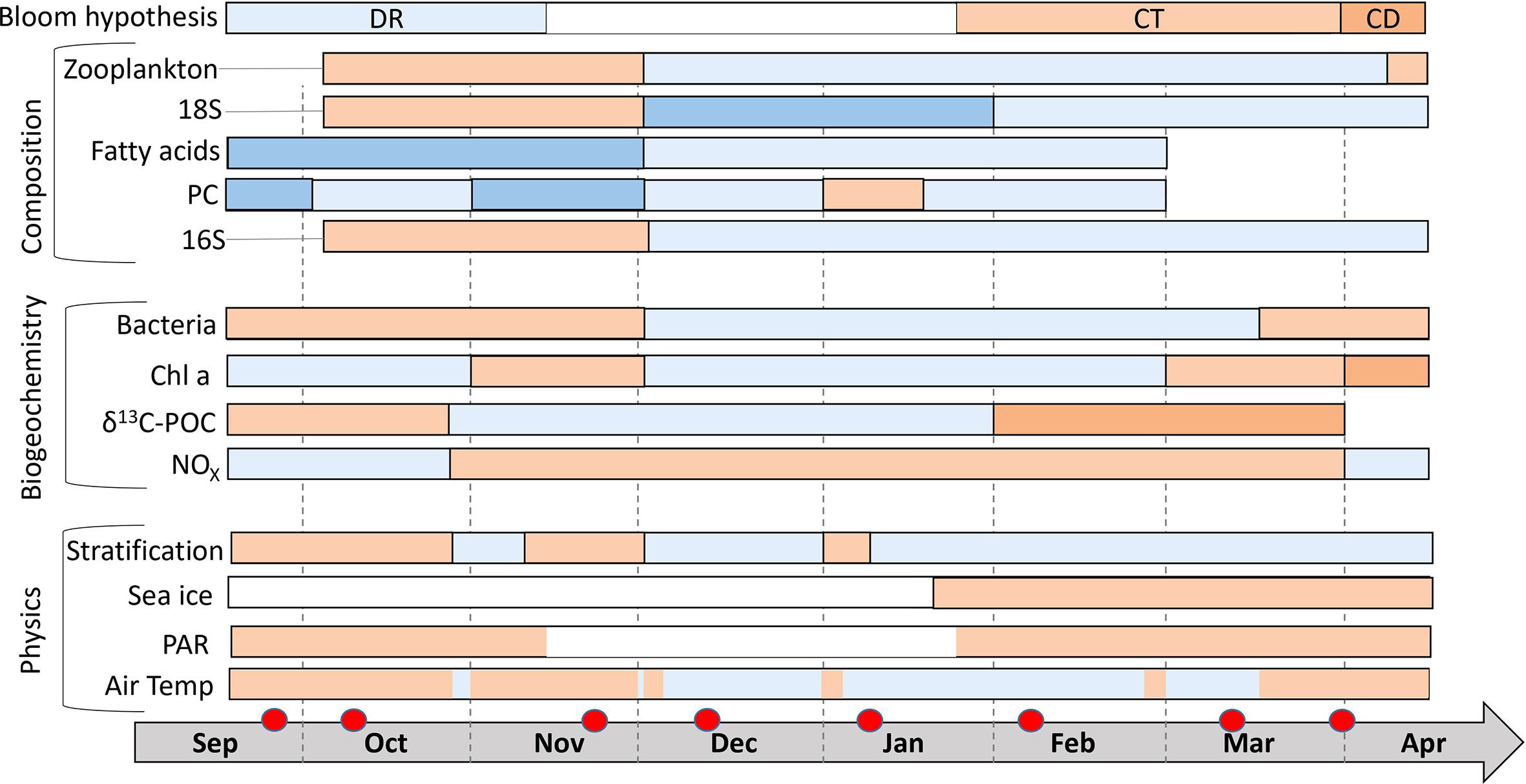
Figure 10 Schematic summary linking selected physical and biogeochemical variables and clustering (composition) of the 16S and 18S communities and Metabolomics data. Air temperatures >0°C are marked in orange and below 0°C in blue. Irradiance (as PAR) is marked in orange if the average daily intensity was >0.5 µE m^-2 s^-2. Sea ice presence at st 1 is marked in orange. Suggested existence of a stratified water column is marked in orange. NO_X concentrations > 4 µmol L^-1 and δ¹³C-POC ratios >-29 ‰ and bacteria abundances above 2 10⁵ cells ml^-1 are marked in orange. Chl concentrations >0.5 mg m^-3 are marked in orange and Chl values > 5 mg m^-3 in dark orange. The composition patterns are indicated based on the NMDS clusters using two to three different colors for the different clusters/compositions. Typical monthly zooplankton biovolumes (Coguiec et al., 2021) above 1 g dw m^-3 are marked in orange and lower values in blue. Red circles indicate the sampling times. Dashed black lines separate months. The bloom hypothesis bar indicates which hypothesis is driving the phytoplankton dynamics leading to autumn and spring blooms (DR: Dilution-recoupling hypothesis, CT: Critical turbulence hypothesis, CD: Critical depth hypothesis, black: light limited).

The main physical drivers were irradiance (photosynthetic active radiation: PAR) and air temperature (+dd). Air temperature was an important factor controlling terrestrial freshwater runoff in autumn and winter (at temperatures above 0°C), which strengthened the land-fjord coupling. During the polar night (PAR <0.5 µE m^-2 s^-2) primary production was light limited, but we found evidence for allochthonous carbon inputs available for bacteria growth. Other drivers such as stratification in the fjord and sea ice cover had a strong local impact especially at st 1. Protist biomass and primary production were also related to nutrient availability and grazing pressure (zooplankton abundances). Autumn had characteristic bacterial and archaeal communities, while the polar night and spring had distinct eukaryotic communities. Fatty acid patterns changed in the same way as the plankton community compositions (DNA-based) which indicates that the fatty acids were mostly originating from the living plankton communities (DNA of dead cells would degrade quickly). In fact, fatty acids are often used as biomarkers for different microalgae groups (Sahu et al., 2014). Polar compound patterns appeared more directly related to meteorological drivers and events than to the biogeochemical parameters or plankton communities. Land-ocean interactions and runoff during rain and melt events functioned as the main source of these compounds. An overview of the data is provided in Figure 10. As discussed above, we suggest different bloom formation hypotheses for the autumn and spring bloom. Our study showed that during the autumn bloom the dilution-recoupling hypothesis (Behrenfeld, 2010) was most important, whereas the spring bloom was controlled by incident solar radiation and to some extend by the critical turbulence (Huisman et al., 1999) and critical depth (Sverdrup, 1953) hypotheses for accumulation of biomass.

The strong environmental changes occurring in coastal systems as shown and predicted by IPCC (2022) suggests major impacts on the coastal marine system. Our results suggest possible change in the timing of the algal autumn bloom, potential failure in currently successful overwintering strategies (due to warming) and stronger decoupling between procaryotic and eukaryotic production dynamics due to stronger land-ocean interactions. Also mid-winter melt events may become more frequent (IPCC, 2022), increasing the overall heterotrophic production during the polar night due to higher terrestrial OM supply. At the same time, higher water temperatures will increase heterotrophic enzymatic activities. Only continued long-term time series studies as done here for Ramfjorden will be able to resolve how the marine system will cope with the multistressor impacts caused by climate change.

Data availability statement

The datasets presented in this study can be found in online repositories. The names of the repository/repositories and accession number(s) can be found below: https://www.ebi.ac.uk/ena, PRJEB40294 https://www.ebi.ac.uk/metabolights/, MTBLS4089 https://dataverse.no/dataset.xhtml?persistentId=doi:10.18710/WG4Y4J, doi.org/10.18710/WG4Y4J.

Author contributions

TV designed the sampling design. TV developed the hypotheses with input from RG, LK and RB. Samples were taken by TV, LK, RB and UD. Algae and bacteria cell counts were done by LK, RB, and TV. Nutrients, phytopigments and POC/PON were measured by RB. Physical data were analysed by TV. DNA extractions were done by TV and UD. TV did the bioinformatics and statistical analyses of the 18S and 16S sequences. RB did the isotopic tracer incubations with support from TV. ¹³C incubations were analysed by GL. Metabolites were extracted by TV and RMB and measured and analysed by DM. The manuscript was prepared by TV and LK with contributions from all co-authors. All authors contributed to the article and approved the submitted version.

Funding

The fieldwork was financed by UiT - The Arctic University of Norway. Other funding was obtained by the ArcticSIZE project - A research group on the productive Marginal Ice Zone at UiT (grant no. 01vm/h15). Additional funding comes from the project FACE-IT (The Future of Arctic Coastal Ecosystems – Identifying Transitions in Fjord Systems and Adjacent Coastal Areas). FACE-IT has received funding from the European Union’s Horizon 2020 research and innovation programme under grant agreement No 869154. Metabolomics lab work and measurement of enriched ¹³C-POC samples was financed by the MPI in Bremen. POM and nutrient analyses were partly financed by the Nordcee group of the Southern Denmark University in Odense.

Acknowledgments

We want to thank the crew of RV Hyas for their invaluable support. We particularly want to thank Frode Gerhardsen, Kunuk Lennart, Ivan Tatone, and Evald Nordli for their skills and company in the field. Lab work was supported by various technicians and colleagues. We specifically want to thank Paul Dubourg, Kristoffer Caspersen, and Ronnie Glud. This work contributes to the Arctic Science Partnership (www.asp-net.org) and the ARCTOS research network (arctos.uit.no). Part of the work has been published as Master thesis of RMB and Bachelor thesis of LK.

Conflict of interest

The authors declare that the research was conducted in the absence of any commercial or financial relationships that could be construed as a potential conflict of interest.

Publisher’s note

All claims expressed in this article are solely those of the authors and do not necessarily represent those of their affiliated organizations, or those of the publisher, the editors and the reviewers. Any product that may be evaluated in this article, or claim that may be made by its manufacturer, is not guaranteed or endorsed by the publisher.

Supplementary material

The Supplementary Material for this article can be found online at: https://www.frontiersin.org/articles/10.3389/fmars.2022.915192/full#supplementary-material

References

Aksnes D. L., Dupont N., Staby A., Fiksen Ø., Kaartvedt S., Aure J. (2009). Coastal water darkening and implications for mesopelagic regime shifts in Norwegian fjords. Mar. Ecol. Prog. Ser. 387, 39–49. doi: 10.3354/meps08120

CrossRef Full Text | Google Scholar

Alonso-Sáez L., Díaz-Pérez L., Morán X. A. G. (2015). The hidden seasonality of the rare biosphere in coastal marine bacterioplankton. Environ. Microbiol. 17 (10), 3766–3780. doi: 10.1111/1462-2920.12801

PubMed Abstract | CrossRef Full Text | Google Scholar

Ardyna M., Arrigo K. R. (2020). Phytoplankton dynamics in a changing Arctic ocean. Nat. Clim. Change. 10, 892–903. doi: 10.1038/s41558-020-0905-y

CrossRef Full Text | Google Scholar

Atienza S., Guardiola M., Præbel K., Antich A., Turon X., Wangensteen O. (2020). DNA Metabarcoding of deep-Sea sediment communities using COI: Community assessment, spatio-temporal patterns and comparison with 18S rDNA. S. Diversity 12 (4), 123. doi: 10.3390/d12040123

CrossRef Full Text | Google Scholar

Behrenfeld M. J. (2010). Abandoning sverdrup's critical depth hypothesis on phytoplankton blooms. Ecology 91 (4), 977–989. doi: 10.1890/09-1207.1

PubMed Abstract | CrossRef Full Text | Google Scholar

Berge J., Daase M., Renaud P. E., Ambrose W. G. Jr., Darnis G., Last K. S., et al. (2015b). Unexpected levels of biological activity during the polar night offer new perspectives on a warming Arctic. Curr. Biol. 25 (19), 2555–2561. doi: 10.1016/j.cub.2015.08.024

PubMed Abstract | CrossRef Full Text | Google Scholar

Berge J., Renaud P. E., Darnis G., Cottier F., Last K., Gabrielsen T. M., et al. (2015a). In the dark: a review of ecosystem processes during the Arctic polar night. Prog. Oceanogr. 139, 258–271. doi: 10.1016/j.pocean.2015.08.005

CrossRef Full Text | Google Scholar

Bourgeois S., Kerhervé P., Calleja M. L., Many G., Morata N. (2016). Glacier inputs influence organic matter composition and prokaryotic distribution in a high Arctic fjord (Kongsfjorden, Svalbard). J. Mar. Syst. 164, 112–127. doi: 10.1016/j.jmarsys.2016.08.009

CrossRef Full Text | Google Scholar

Boyer F., Mercier C., Bonin A., Le Bras Y., Taberlet P., Coissac E. (2016). Obitools: A unix-inspired software package for DNA metabarcoding. Mol. Ecol. Resour. 16 (1), 176–182. doi: 10.1111/1755-0998.12428

PubMed Abstract | CrossRef Full Text | Google Scholar

Cheng L., Normandeau C., Bowden R., Doucett R., Gallagher B., Gillikin D. P., et al. (2019). An international intercomparison of stable carbon isotope composition measurements of dissolved inorganic carbon in seawater. Limnol. Oceanogr. Meth. 17 (3), 200–209. doi: 10.1002/lom3.10300

CrossRef Full Text | Google Scholar

Christman G. D., Cottrell M. T., Popp B. N., Gier E., Kirchman D. (2011). Abundance, diversity, and activity of ammonia-oxidizing prokaryotes in the coastal Arctic ocean in summer and winter. L. Appl. Environ. Microbiol. 77 (6), 2026–2034. doi: 10.1128/AEM.01907-10

CrossRef Full Text | Google Scholar

Cleary A. C., Durbin E. G. (2016). Unexpected prevalence of parasite 18S rDNA sequences in winter among Antarctic marine protists. J. Plankton Res. 38 (3), 401–417. doi: 10.1093/plankt/fbw005

CrossRef Full Text | Google Scholar

Coguiec E., Daase M., Ershova E. A., Vonnahme T., Wangensteen O. S., Gradinger R., et al. (2021). Seasonal variability in the zooplankton community structure in a sub-Arctic fjord as revealed by morphological and molecular approaches. Front. Mar. Sci. 1049. doi: 10.3389/fmars.2021.705042

CrossRef Full Text | Google Scholar

Cottier F. R., Nilsen F., Skogseth R., Tverberg V., Skarðhamar J., Svendsen H. (2010). Arctic Fjords: a review of the oceanographic environment and dominant physical processes. Geological Society London Special Publications 344 (1), 35–50. doi: 10.1144/SP344.4

CrossRef Full Text | Google Scholar

Davis J., Benner R. (2005). Seasonal trends in the abundance, composition and bioavailability of particulate and dissolved organic matter in the Chukchi/Beaufort seas and western Canada basin. Deep Sea Res. Part II Top. Stud. Oceanogr. 52 (24-26), 3396–3410. doi: 10.1016/j.dsr2.2005.09.006

CrossRef Full Text | Google Scholar

Degerlund M., Eilertsen H. C. (2010). Main species characteristics of phytoplankton spring blooms in NE Atlantic and Arctic waters (68–80 n). Estuaries coasts. 33 (2), 242–269. doi: 10.1007/s12237-009-9167-7

CrossRef Full Text | Google Scholar

Delpech L. M., Vonnahme T. R., McGovern M., Gradinger R., Præbel K., Poste A. E. (2021). Terrestrial inputs shape coastal bacterial and archaeal communities in a high Arctic fjord (Isfjorden, Svalbard). Front. Microbiol. 12, 295. doi: 10.3389/fmicb.2021.614634

CrossRef Full Text | Google Scholar

Eilertsen H. C., Taasen J. P. (1984). Investigations on the plankton community of Balsfjorden, Northern. Norway The phytoplankton 1976–1978. Environmental factors, dynamics of growth, and primary production. Sarsia 69, 1–15. doi: 10.1080/00364827.1984.10420584

CrossRef Full Text | Google Scholar

Eilertsen H. C. (1993). Spring blooms and stratification. Nature 363 (6424), 24–24. doi: 10.1038/363024a0

PubMed Abstract | CrossRef Full Text | Google Scholar

Eilertsen H. C., Degerlund M. (2010). Phytoplankton and light during the northern high-latitude winter. J. Plankton Res. 32 (6), 899–912. doi: 10.1093/plankt/fbq017

CrossRef Full Text | Google Scholar

Eilertsen H. C., Frantzen S. (2007). Phytoplankton from two sub-Arctic fjords in northern Norway 2002–2004: I. seasonal variations in chlorophyll a and bloom dynamics. Mar. Biol. Res. 3 (5), 319–332. doi: 10.1080/17451000701632877

CrossRef Full Text | Google Scholar

Eilertsen H. C., Schei B., Taasen J. P. (1981). Investigations on the plankton community of bals-fjorden, northern Norway: The phytoplankton 1976–1978. abundance, species composition, and succession. Sarsia 66 (2), 129–141. doi: 10.1080/00364827.1984.10420584

CrossRef Full Text | Google Scholar

Eilertsen H. C., Taasen J. P., WesIawski J. M. (1989). Phytoplankton studies in the fjords of West spitzbergen: physical environment and production in spring and summer. J. Plankton Res. 11 (6), 1245–1260. doi: 10.1093/plankt/11.6.1245

CrossRef Full Text | Google Scholar

Esteves F. A. (1998). Foundations of limnology (in Portuguese) (Rio de Janeiro: Intercieˆncia).

Google Scholar

Figueroa D., Rowe O. F., Paczkowska J., Legrand C., Andersson A. (2016). Allochthonous carbon–a major driver of bacterioplankton production in the subarctic northern Baltic Sea. Microb. Ecol. 71 (4), 789–801. doi: 10.1007/s00248-015-0714-4

PubMed Abstract | CrossRef Full Text | Google Scholar

Finley A., Banerjee S., Hjelle Ø, Bivand R. (2017). Package ‘MBA’ v0.0-9, multilevel b-spline approximation, CRAN repository. Available at: https://CRAN.R-project.org/package=MBA. 07-04-2022.

Google Scholar

French J. (2017). Autoimage: Multiple heat maps for projected coordinates. R J. 9, 284–297. doi: 10.32614/RJ-2017-025

PubMed Abstract | CrossRef Full Text | Google Scholar

Good S. A., Martin M. J., Rayner N. A. (2013). EN4: quality controlled ocean temperature and salinity profiles and monthly objective analyses with uncertainty estimates. J. Geophys. Res. Oceans. 118, 6704–6716. doi: 10.1002/2013JC009067

CrossRef Full Text | Google Scholar

Grasshoff K., Kremling K., Ehrhardt M. (2009). Methods of seawater analysis (Weinheim; New York; Chiestr; Brisbane; Singapore; Toronto: John Wiley and Sons).

Google Scholar

Großkopf T., Mohr W., Baustian T., Schunck H., Gill D., Kuypers M. M., et al. (2012). Doubling of marine dinitrogen-fixation rates based on direct measurements. Nature 488 (7411), 361–364. doi: 10.1038/nature11338

PubMed Abstract | CrossRef Full Text | Google Scholar

Guardiola M., Uriz M. J., Taberlet P., Coissac E., Wangensteen O. S. (2015). And turon, x.: Deep-sea, deep-sequencing: metabarcoding extracellular DNA from sediments of marine canyons. PloS One 10 (10), e0139633. doi: 10.3390/d12040123

PubMed Abstract | CrossRef Full Text | Google Scholar

Hameed A., Shahina M., Lin S. Y., Lai W. A., Hsu Y. H., Liu Y. C., et al. (2014). Aquibacter zeaxanthinifaciens gen. nov., sp. nov., a zeaxanthin-producing bacterium of the family flavobacteriaceae isolated from surface seawater, and emended descriptions of the genera Aestuariibaculum and Gaetbulibacter. Int. J. Syst. 64, 138–145. doi: 10.1099/ijs.0.052621-0

CrossRef Full Text | Google Scholar

Hasle G. R., Syvertsen E. E., Steidinger K. A., Tangen K., Tomas C. R. (1996). Identifying marine diatoms and dinoflagellates (San Diego, New York, Boston, London, Sydney, Tokyo, Toronto: Elsevier).

Google Scholar

Hegseth E. N., Assmy P., Wiktor J. M., Wiktor J., Kristiansen S., Leu E., et al. (2019). Phytoplankton seasonal dynamics in kongsfjorden, Svalbard and the adjacent shelf. In Ecosystem Kongsfjorden Svalbard (Cham) 2, 173–227. doi: 10.1007/978-3-319-46425-1_6

CrossRef Full Text | Google Scholar

Higashioka Y., Kojima H., Watanabe M., Fukui M. (2013). Desulfatitalea tepidiphila gen. nov., sp. nov., a sulfate-reducing bacterium isolated from tidal flat sediment. Int. J. Syst. 63 (Pt_2), 761–765. doi: 10.1099/ijs.0.043356-0

CrossRef Full Text | Google Scholar

Huang B. C., Banzon V., Freeman E., Graham G., Hankins B., Smith T., et al. (2020). Improvements of the daily optimum interpolation Sea surface temperature (DOISST) version 2.1. J. Clim. 34, 2923–2939. doi: 10.1175/JCLI-D-20-0166.1

CrossRef Full Text | Google Scholar

Huisman J., van Oostveen P., Weissing F. J. (1999). Critical depth and critical turbulence: Two different mechanisms for the development of phytoplankton blooms. Limnol. Oceanogr. 44(7), 1781–1787. doi: 10.4319/lo.1999.44.7.1781

CrossRef Full Text | Google Scholar

IPCC (2022). "Climate change 2022: Impacts, adaptation and vulnerability". in Contribution of working group II to the sixth assessment report of the Intergovernmental Panel on Climate Change". Eds.Pörtner H.-O., Roberts D.C., Tignor M., Poloczanska E.S., Mintenbeck K., Alegría A., et al (Cambridge, UK and New York, NY, USA:Cambridge University Press), 3056.

Google Scholar

Iversen K. R., Seuthe L. (2011). Seasonal microbial processes in a high-latitude fjord (Kongsfjorden, svalbard): I. heterotrophic bacteria, picoplankton and nanoflagellates. Polar Biol. 34 (5), 731–749. doi: 10.1007/s00300-010-0929-2

CrossRef Full Text | Google Scholar

Jespersen A. M., Christoffersen K. (1987). Measurements of chlorophyll―a from phytoplankton using ethanol as extraction solvent. Archiv für Hydrobiol. 109 (3), 445–454.

Google Scholar

Johnsen G., Leu E., Gradinger R. (2020). Marine micro-and macroalgae in the polar night. in polar night marine ecology (Cham: Springer), 67–112.

Google Scholar

Kaiser K., Canedo-Oropeza M., McMahon R., Amon R. M. (2017). Origins and transformations of dissolved organic matter in large Arctic rivers. Sci. Rep. 7 (1), 1–11. doi: 10.1038/s41598-017-12729-1

PubMed Abstract | CrossRef Full Text | Google Scholar

Kartverket. Available at: https://kartkatalog.geonorge.no/metadata/kartverket/dybdedata/2751aacf-5472-4850-a208-3532a51c529a (Accessed 10 August 2020).

Google Scholar

Kumar V., Tiwari M., Nagoji S., Tripathi S. (2016). Evidence of anomalously low δ13C of marine organic matter in an Arctic fjord. Sci. Rep. 6 (1), 1–9. doi: 10.1038/srep36192

PubMed Abstract | CrossRef Full Text | Google Scholar

Kume A., Koyata H., Sakakibara T., Ishiguro Y., Kure S., Hiraga K. (1991). The glycine cleavage system. molecular cloning of the chicken and human glycine decarboxylase cDNAs and some characteristics involved in the deduced protein structures. JBC 266 (5), 3323–3329. doi: 10.1016/S0021-9258(18)49991-7

CrossRef Full Text | Google Scholar

Kvernvik A. C., Hoppe C. J. M., Lawrenz E., Prášil O., Greenacre M., Wiktor J. M., et al. (2018). Fast reactivation of photosynthesis in arctic phytoplankton during the polar night. J. Phycol. 54 (4), 461–470. doi: 10.1111/jpy.12750

PubMed Abstract | CrossRef Full Text | Google Scholar

Larsen A., Flaten G. A. F., Sandaa R. A., Castberg T., Thyrhaug R., Erga S. R., et al. (2004). Spring phytoplankton bloom dynamics in Norwegian coastal waters: microbial community succession and diversity. Limnol. Oceanogr. 49 (1), 180–190. doi: 10.4319/lo.2004.49.1.0180

CrossRef Full Text | Google Scholar

Lau K. W., Ng C. Y., Ren J., Lau S. C., Qian P. Y., Wong P. K., et al. (2005). Owenweeksia hongkongensis gen. nov., sp. nov., a novel marine bacterium of the phylum ‘Bacteroidetes’. Int. J. Syst. 55 (3), 1051–1057. doi: 10.1099/ijs.0.63155-0

CrossRef Full Text | Google Scholar

Lee S., Wolberg G., Shin S. Y. (1997). Scattered data interpolation with multilevel b-splines, IEE transactions on visualization and computer graphics. IEEE 3 (3), 229–224. doi: 10.1109/2945.620490

CrossRef Full Text | Google Scholar

López-Sandoval D. C., Delgado-Huertas A., Agustí S. (2018). The 13C method as a robust alternative to 14C-based measurements of primary productivity in the Mediterranean Sea. J. Plankton Res. 40 (5), 544–554. doi: 10.1093/plankt/fby031

PubMed Abstract | CrossRef Full Text | Google Scholar

Mahé F., Rognes T., Quince C., de Vargas C., Dunthorn M. (2014). Swarm: robust and fast clustering method for amplicon-based studies. PeerJ 2, e593. doi: 10.7717/peerj.593

PubMed Abstract | CrossRef Full Text | Google Scholar

Marquardt M., Vader A., St¨ubner E. I., Reigstad M., Gabrielsen T. M. (2016). Strong seasonality of marine microbial eukaryotes in a high-arctic fjord (Isfjorden, in West spitsbergen, Norway). Appl. Environ. Microbiol. 82 (6), 1868–1880. doi: 10.1128/AEM.03208-15

PubMed Abstract | CrossRef Full Text | Google Scholar

Matthews J. B. L., Heimdal B. R. (1980). “Pelagic productivity and food chains in fjord systems,” in Fjord oceanography (Boston, MA: Springer), (pp. 377–398).

Google Scholar

McGovern M., Pavlov A. K., Deininger A., Granskog M. A., Leu E., Søreide J. E., et al. (2020). Terrestrial Inputs Drive Seasonality in Organic Matter and Nutrient Biogeochemistry in a High Arctic Fjord System (Isfjorden, Svalbard). Front. Mar. Sci. 7, 542563. doi: 10.3389/fmars.2020.542563

CrossRef Full Text | Google Scholar

Monier A., Terrado R., Thaler M., Comeau A., Medrinal E., Lovejoy C. (2013). Upper Arctic ocean water masses harbor distinct communities of heterotrophic flagellates. Biogeosciences 10 (6), 4273–4286. doi: 10.5194/bg-10-4273-2013

CrossRef Full Text | Google Scholar

Morris R. M., Rappé M. S., Connon S. A., Vergin K. L., Siebold W. A., Carlson C. A., et al. (2002). SAR11 clade dominates ocean surface bacterioplankton communities. Nature 420 (6917), 806–810. doi: 10.1038/nature01240

PubMed Abstract | CrossRef Full Text | Google Scholar

Müller O., Seuthe L., Bratbak G., Paulsen M. L. (2018). Bacterial response to permafrost derived organic matter input in an Arctic fjord. Front. Mar. Sci. 5, 263. doi: 10.3389/fmars.2018.00263

CrossRef Full Text | Google Scholar

Norsk Klimaservicesenter. Available at: https://seklima.met.no/ (Accessed 31st of August 2022).

Google Scholar

Opdal A. F., Lindemann C., Aksnes D. L. (2019). : Centennial decline in north Sea water clarity causes strong delay in phytoplankton bloom timing. Glob 25 (11), 3946–3953. doi: 10.1111/gcb.14810

CrossRef Full Text | Google Scholar

Orata F. (2012). Derivatization reactions and reagents for gas chromatography analysis. advanced gas chromatography-progress in agricultural, biomedical and industrial applications. J. Mar. Syst. 91, 122–127. doi: 10.5772/33098

CrossRef Full Text | Google Scholar

O’Sadnick M., Petrich C., Brekke C., Skarðhamar J. (2020). Ice extent insub-arctic fjords and coastal areas from 2001to 2019 analyzed from MODIS imagery. Ann. Glaciol. 61 (82), 1–17. doi: 10.1017/aog.2020.34

CrossRef Full Text | Google Scholar

Parada A. E., Needham D. M., Fuhrman J. A. (2016). Every base matters: assessing small subunit rRNA primers for marine microbiomes with mock communities, time series and global field samples. Environ. Microbiol. 18 (5), 1403–1414. doi: 10.1111/1462-2920.13023

PubMed Abstract | CrossRef Full Text | Google Scholar

Parsons T. R., Maita Y., Lalli C. M. (Eds.) (1984). Manual of chemical and biological methods for seawater analysis (Toronto: Pergamon Press).

Google Scholar

Persson E. (2020). Spring sea ice algal development in the sub-Arctic ramfjorden (northern Norway: Master's thesis, UiT Norges arktiske universitet).

Google Scholar

Porter K. G., Feig Y. S. (1980). The use of DAPI for identifying and counting aquatic microflora. Limnol. Oceanogr. 25, 943–885.948. doi: 10.4319/lo.1980.25.5.0943

CrossRef Full Text | Google Scholar

Randelhoff A., Holding J., Janout M., Sejr M. K., Babin M., Tremblay J-É., et al. (2020). Pan-arctic ocean primary production constrained by turbulent nitrate fluxes. Front. Mar. Sci. 7, 150. doi: 10.3389/fmars.2020.00150

CrossRef Full Text | Google Scholar

Regaudie-de-Gioux A., Lasternas S., Agustí S., Duarte C. M. (2014). Comparing marine primary production estimates through different methods and development of conversion equations. Front. Mar. Sci. 1, 19. doi: 10.3389/fmars.2014.00019

CrossRef Full Text | Google Scholar

Roden V. J., Kocsis Á. T., Zuschin M., Kiessling W. (2018). Reliable estimates of beta diversity with incomplete sampling. Ecology 99 (5), 1051–1062. doi: 10.1002/ecy.2201

PubMed Abstract | CrossRef Full Text | Google Scholar

Sahu A., Pancha I., Jain D., Paliwal C., Ghosh T., Patidar S., et al. (2014). Fatty acids as biomarkers of microalgae. Phytochemistry 89, 53–58. doi: 10.1016/j.phytochem.2013.02.001

CrossRef Full Text | Google Scholar

Saiz E., Calbet A., Isari S., Anto M., Velasco E. M., Almeda R., et al. (2013). Zooplankton distribution and feeding in the Arctic ocean during a phaeocystis pouchetii bloom. Deep Sea Res. Part I Oceanogr. Res. 72, 17–33. doi: 10.1016/j.dsr.2012.10.003

CrossRef Full Text | Google Scholar

Shantha N. C., Napolitano G. E. (1992). Gas chromatography of fatty acids. J. Chromatogr. A 624 (1-2), 37–51. doi: 10.1016/0021-9673(92)85673-H

CrossRef Full Text | Google Scholar

Sherr E. B., Sherr B. F., Hartz A. J. (2009). Microzooplankton grazing impact in the Western Arctic ocean. Deep Sea Res. Part II Top. Stud. Oceanogr. 56 (17), 1264–1273. doi: 10.1016/j.dsr2.2008.10.036

CrossRef Full Text | Google Scholar

Simenstad C. A., Wissmar R. C. (1985). d13C evidence of the origins and fates of organic carbon in estuarine and nearshore food webs. Mar. Ecol. Prog. Ser. 22, 141–152. doi: 10.3354/meps022141

CrossRef Full Text | Google Scholar

Sipler R. E., Baer S. E., Connelly T. L., Frischer M. E., Roberts Q. N., Yager P. L., et al. (2017a). Chemical and photophysiological impact of terrestrially-derived dissolved organic matter on nitrate uptake in the coastal western Arctic. Limnol. Oceanogr. 62 (5), 1881–1894. doi: 10.1002/lno.10541

CrossRef Full Text | Google Scholar

Sipler R. E., Kellogg C. T., Connelly T. L., Roberts Q. N., Yager P. L., Bronk D. A. (2017b). Microbial community response to terrestrially derived dissolved organic matter in the coastal arctic. Front. Microbiol. 8, 1018. doi: 10.3389/fmicb.2017.01018

PubMed Abstract | CrossRef Full Text | Google Scholar

Smayda T. J., Mitchell-Innes B. (1974). Dark survival of autotrophic, planktonic marine diatoms. Mar. Biol. 25 (3), 195–202. doi: 10.1007/BF00394965

CrossRef Full Text | Google Scholar

Stenow R., Olofsson M., Robertson E. K., Kourtchenko O., Whitehouse M. J., Ploug H., et al. (2020). Resting stages of skeletonema marinoi assimilate nitrogen from the ambient environment under dark, anoxic conditions. J. Phycol. 56 (3), 699–708. doi: 10.1111/jpy.12975

PubMed Abstract | CrossRef Full Text | Google Scholar

Sverdrup H. U. (1953). On conditions for the vernal blooming of phytoplankton. Cons. Perm. Int. Expl. Mer. 18, 287–295. doi: 10.1093/icesjms/18.3.287

CrossRef Full Text | Google Scholar

Teeling H., Fuchs B. M., Bennke C. M., Krueger K., Chafee M., Kappelmann L., et al. (2016). Recurring patterns in bacterioplankton dynamics during coastal spring algae blooms. elife 5, e11888. doi: 10.7554/eLife.11888

PubMed Abstract | CrossRef Full Text | Google Scholar

Throndsen J., Hasle G. R., Tangen K. (Eds.) (2007). Phytoplankton of Norwegian coastal waters (Oslo, Norway: Almater Forlag AS).

Google Scholar

Tomas C. R. (Ed.) (1997). Identifying marine phytoplankton (San Diego: Elsevier).

Google Scholar

Turner Designs (2006). Trilogy laboratory fluorometer user’s manual version 1.7. 1–41.

Google Scholar

Utermöhl H. (1958). Methods of collecting plankton for various purposes are discussed. SIL Commun. 1953 1996. 9, 1–38. doi: 10.1080/05384680.1958.11904091

CrossRef Full Text | Google Scholar

Verity P. G., Vernet M. (1992). Microzooplankton grazing, pigments, and composition of plankton communities during late spring in two Norwegian fjords. Sarsia 77 (3-4), 263–274. doi: 10.1080/00364827.1992.10413511

CrossRef Full Text | Google Scholar

Vonnahme T. R., Leroy M., Thoms S., van Oevelen D., Harvey H. R., Kristiansen S., et al. (2021a). Modeling silicate–nitrate–ammonium co-limitation of algal growth and the importance of bacterial remineralization based on an experimental Arctic coastal spring bloom culture study. Biogeosciences 18 (5), 1719–1747. doi: 10.5194/bg-18-1719-2021

CrossRef Full Text | Google Scholar

Vonnahme T. R., Persson E., Dietrich U., Hejdukova E., Dybwad C., Elster, et al. (2021b). Early spring subglacial discharge plumes fuel under-ice primary production at a Svalbard tidewater glacier. TC 15 (4), 2083–2107. doi: 10.5194/tc-15-2083-2021

CrossRef Full Text | Google Scholar

Walker C. B., de la Torre J. R., Klotz M. G., Urakawa H., Pinel N., Arp D. J., et al. (2010). Nitrosopumilus maritimus genome reveals unique mechanisms for nitrification and autotrophy in globally distributed marine crenarchaea. Proc. Natl. Acad. Sci. 107 (19), 8818–8823. doi: 10.1073/pnas.0913533107

CrossRef Full Text | Google Scholar

Wangensteen O. S., Palacín C., Guardiola M., Turon X. (2018). DNA Metabarcoding of littoral hard-bottom communities: high diversity and database gaps revealed by two molecular markers. PeerJ 6, e4705. doi: 10.7717/peerj.4705

PubMed Abstract | CrossRef Full Text | Google Scholar

Wang Q., Garrity G. M., Tiedje J. M., Cole J. R. (2007). Naive Bayesian classifier for rapid assignment of rRNA sequences into the new bacterial taxonomy. Appl. Environ. Microbiol. 73 (16), 5261–5267. doi: 10.1128/AEM.00062-07

PubMed Abstract | CrossRef Full Text | Google Scholar

Wietz M., Bienhold C., Metfies K., Torres-Valdés S., von Appen W. J., Salter I., et al. (2021). The polar night shift: Seasonal dynamics and drivers of Arctic Ocean microbiomes revealed by autonomous sampling. ISME Commun. 1 (1), 1–12. doi: 10.1038/s43705-021-00074-4

CrossRef Full Text | Google Scholar

Wihsgott J. U., Sharples J., Hopkins J. E., Woodward E. M. S., Hull T., Greenwood N., et al. (2019). Observations of vertical mixing in autumn and its effect on the autumn phytoplankton bloom. Prog. Oceanogr. 177, 102059. doi: 10.1016/j.pocean.2019.01.001

CrossRef Full Text | Google Scholar

Wunder L. C., Aromokeye D. A., Yin X., Richter-Heitmann T., Willis-Poratti G., Schnakenberg A., et al. (2021). Iron and sulfate reduction structure microbial communities in (sub-) Antarctic sediments. ISME J. 15, 1–18. doi: 10.1038/s41396-021-01014-9

PubMed Abstract | CrossRef Full Text | Google Scholar

Yamamoto E., Muramatsu H., Nagai K. (2014). Vulgatibacter incomptus gen. nov., sp. nov. and labilithrix luteola gen. nov., sp. nov., two myxobacteria isolated from soil in yakushima island, and the description of vulgatibacteraceae fam. nov., labilitrichaceae fam. nov. and anaeromyxobacteraceae fam. nov. Int. J. Syst. Evol. 64 (Pt_10), 3360–3368. doi: 10.1099/ijs.0.063198-0

CrossRef Full Text | Google Scholar

Yang E. J., Ha H. K., Kang S. H. (2015). Microzooplankton community structure and grazing impact on major phytoplankton in the chukchi sea and the western Canada basin. Arctic ocean. Deep Sea Res. Part II Top. Stud. Oceanogr. 120, 91–102. doi: 10.1016/j.dsr2.2014.05.020

CrossRef Full Text | Google Scholar

Yergeau E., Michel C., Tremblay J., Niemi A., King T. L., Wyglinski J., et al. (2017). Metagenomic survey of the taxonomic and functional microbial communities of seawater and sea ice from the Canadian Arctic. Sci. Rep. 7, 42242. doi: 10.1038/srep42242

PubMed Abstract | CrossRef Full Text | Google Scholar

Yr.no, Tromsø Verværslinga. Available at: https://www.yr.no/nb/historikk/graf/5-90450/Norge/Troms%20og%20Finnmark/Troms%C3%B8/Troms%C3%B8%20(Vervarslinga) (Accessed 08.12.2020).

Google Scholar

Zhang Q., Gradinger R., Spindler M. (1998). Dark survival of marine microalgae in the high Arctic (Greenland Sea). Polarforschung 65 (3), 111–116.

Google Scholar