Application of multi-regression machine learning algorithms to solve ocean water mass mixing in the Atlantic Ocean

The distribution of any non-conservative variable in the deep open ocean results from the circulation and mixing of water masses (WMs) of contrasting origin and from the initial preformed composition, modified during ongoing simultaneous biological and/or geochemical processes. Estimating the contribution of the WMs composing a sample is useful to trace the distribution of each water mass and to quantitatively separate the physical (mixing) and biogeochemical components of the variability of any, non- conservative variable (e.g., dissolved organic carbon, prokaryote biomass) in the ocean. Other than potential temperature and salinity, additional semi-conservative and non-conservative variables have been used to solve the mixing of more than three water masses using Optimum Multi-Parameter (OMP) approaches. Successful application of an OMP analysis requires knowledge of the characteristics of the water masses in their source regions as well as their circulation and mixing patterns. Here, we propose the application of multi-regression machine learning models to solve ocean water mass mixing. The models tested were trained using the solutions from OMP analyses previously applied to samples from cruises in the Atlantic Ocean. Extremely Randomized Trees algorithm yielded the highest score (R^{2 =} 0.9931; mse = 0.000227). Our model allows solving the mixing of water masses in the Atlantic Ocean using potential temperature, salinity, latitude, longitude and depth. Therefore, basic hydrographic data collected during typical research cruises or autonomous systems can be used as input variables and provide results in real time. The model can be fed with new solutions from compatible OMP analyses as well as with new water masses not previously considered in it. Our tool will provide knowledge on water mass composition and distribution to a broader community of marine scientists not specialized in OMP analysis and/or in the oceanography of the studied area. This will allow a quantitative analysis of the effect of water mass mixing on the variables or processes under study.

Introduction

Determining the contribution of the water masses composing a water sample is useful to trace the basin-wide distribution of each water mass, to define its core-of flow identifying the depth of maximum water mass contribution or the depth-range where the water mass is dominant contributing > 50% (e.g. Álvarez et al., 2014). Ocean biogeochemists and microbiologists can also benefit from this knowledge to obtain water mass weighted average concentrations of the studied variables or basin-wide trends along cores-of-flow. Even more interesting is the possibility of estimating the impact of water mass mixing on the variability of any chemical (e.g. inorganic nutrients and dissolved organic carbon; Álvarez-Salgado et al., 2014 and Romera-Castillo et al., 2019, respectively) or biological (e.g. prokaryotic heterotrophic abundance and production; Reinthaler et al., 2013) property. In this regard the distribution of any non-conservative variable N in the deep open ocean results from the circulation and mixing of water masses of contrasting origin and initial preformed composition, modified during ongoing simultaneous biological and/or geochemical processes, which add or remove that particular property. Therefore, to isolate the, usually small, variability due to biogeochemical processes (ΔN), the influence of water mass mixing (usually dominant) is needed to be removed:

$$N_i={\displaystyle \sum _j{a}_j·x_{ij}}+\Delta N_i$$

Where N_i and ΔN_i are the measured and residual (mixing removed) concentration of N in sample i; x_ij is the proportion of water mass j in sample i; and a_j s the coefficient of the multiple linear correlation of N_i with x_ij. Therefore, we need to know the contribution of each water mass to each sample. This is not an easy task and requires expertise on the origin, circulation and mixing patterns of the water masses present in the study area. The most commonly used methodology is the Optimum Multi-Parameter (OMP) analysis that was first applied by Tomczak (1981). This methodology resolves a system of n linear mass balance equations with n+1 unknowns and two constraints: i) the sum of all the water mass proportions must be equal to 1 ( ∑_jx_ij=1 ), and ii) all the water mass proportions must be positive. The OMP can be run in conservative mode, which includes mass balance equations ( C_i=Σ_j C_j·x_ij ) for potential temperature, salinity, conservative (e.g. ‘NO’ and ‘PO’) and semi-conservative chemical parameters (e.g. silicate, Álvarez et al., 2014). It can also be run in non-conservative mode, extended OMP, including potential temperature, salinity, dissolved oxygen, nitrate and phosphate (e.g. Poole and Tomczak, 1999; Pardo et al., 2012). In this case, fixed stoichiometric ratios relating dissolved oxygen and inorganic nutrients are imposed and an extra unknown, dissolved oxygen consumption (ΔO₂) has to be added to the set of linear mass balance equations. In any case, the mixing of a maximum of six water masses could be solved with these equations using temperature, salinity and non-conservative tracers (nitrate, phosphate and oxygen) when, for instance, the deep Atlantic Ocean is a mosaic of more than 15 water masses (Romera-Castillo et al., 2019). Therefore, additional oceanographic criteria based on the density and proximity of water masses have to be applied to define mixing clusters and solve the mixing for each cluster. In summary, an OMP analysis demands availability of a large set of quality-controlled chemical variables together with a deep knowledge of the oceanography of the studied area. Moreover, those chemical variables are not always available or do not have the required quality by contrast to potential temperature and salinity that are high standard core variables in any cruise or database. Therefore, resolving the water mass mixing with an OMP analysis usually takes a large fraction of the time needed to answer a biogeochemical question.

Moreover, for the study of water masses formation, mixing, mineralization and transport, it is necessary to combine water column high quality ship-based thermohaline and discrete essential biogeochemical (BGC) data. These essential BGC data are considered level 1 priority in traditional hydrographic cruises (https://www.go-ship.org/DatReq.html) and require an inversion in equipment, analytical reagents (including reference materials) and data processing time by highly trained technical personnel. Discrete BGC data are also useful to calibrate sensor-based data from autonomous BGC platforms, offering a much wider temporal and spatial coverage in the upper 2000 meters. The more extensive use of these platforms leads to new capabilities and challenges regarding biogeochemical processes and ecosystem dynamics in the ocean (Claustre and Johnson, 2016).

Within this context of new challenges to be solved in oceanography, Machine learning (ML) is being increasingly used in a variety of applications including ocean weather and climate predictions, coastal water monitoring, habitat modelling and distribution, species identification, marine resources management, detection of oil spill and pollution and wave modelling (Ahmad, 2019). ML has been also applied in some biogeochemical studies. For instance, it has identified a link between warming and a reduction in primary production in the North Atlantic Gyre (D’Alelio et al., 2020). Also, the use of neural networks has been applied to estimate open ocean CO₂ and inorganic nutrient concentrations (Bittig et al., 2018). The main advantage of ML techniques applied to oceanography is that they can help oceanographers in those processes that involve taking decisions or making predictions based on data. Nowadays, there is an increasing set of big, diverse, curated oceanographic databases, and additionally, multiple ML approaches to several problems have provided a profusion of techniques that can be adapted to very different fields.

The aim of this work is to apply a supervised ML approach to solve water mass mixing, evaluating several algorithms that are applicable in this situation. To do so, we have used a database compiling several cruises in the Atlantic Ocean including the water mass composition of every sample obtained with an OMP analysis. Besides, we added samples from areas where the water masses were formed (100% proportion) from the GLODAPv2.2020 database (Olsen et al., 2020). Using only potential temperature and salinity, we have validated our ML algorithm against the results from the OMP analysis with a low error, showing the usefulness of the ML approach. We also provide the algorithm so any user can download it and easily apply it to determine the water mass composition of any sample in the Atlantic Ocean.

Material and methods

Data selection

In order to train and test our models, we needed a database of labeled data, i.e. a collection of water samples such that we know the contribution of each water mass for every sample. For that, we used a database previously analysed in Romera-Castillo et al. (2019). Briefly, the database, consisting of 11,245 samples, was composed of U.S. Global Ocean Carbon and Repeat Hydrography cruises, covering the whole Atlantic Ocean (Figure 1) and identified with the following alias and expocode numbers (in brackets): A13.5 (33RO20100308), A22 (33AT20120324, excluding data from the Caribbean Sea), A20 (33AT20120419), A16N (33RO20130803), A16S (33RO20131223) and A10 (33RO20110926). An OMP analysis was applied to those cruise data below 250m and potential temperature lower than 14°C. Both the database and the results of the OMP analysis can be found in PANGAEA (https://doi.pangaea.de/10.1594/PANGAEA.904326). Three additional data transect not included in the OMP analysis were used to test the model: A9.5 (740H20180228), A25 (35TH20080610) and A03 (74AB20050501). In our ML approach, other than the contribution of each water mass, we used location (Latitude, Longitude and depth), potential temperature and salinity, for each sample.

FIGURE 1

Figure 1 Location of the sections included in the PANGAEA database (A16, A20, A22, A10 and A13.5, in blue) and three extra sections (A9.5, A25 and A03, in red) used in this study to test the model. Figure plotted with the Ocean Data View software (Schlitzer, 2015).

We also used a set of 2,920 samples (Table 1) from the GLODAPv2 database (Olsen et al., 2020) which had a 100% contribution of each water mass (pure water masses database), i.e., they were located where the water mass was formed according to the characteristic potential temperature and salinity ranges described in Romera-Castillo et al. (2019) as well as latitude, longitude and depth from previous works (Romera-Castillo et al., 2019; Liu and Tanhua, 2021). This set of samples, hereinafter pure water masses dataset (pure WMs), gave robustness to the algorithm since they coincide with the characteristics of the water masses in their formation areas (source water types) used to run the OMP analysis (Romera-Castillo et al., 2019) and, in some cases, they are not contained in the hydrographic sections composing the OMP database.

TABLE 1

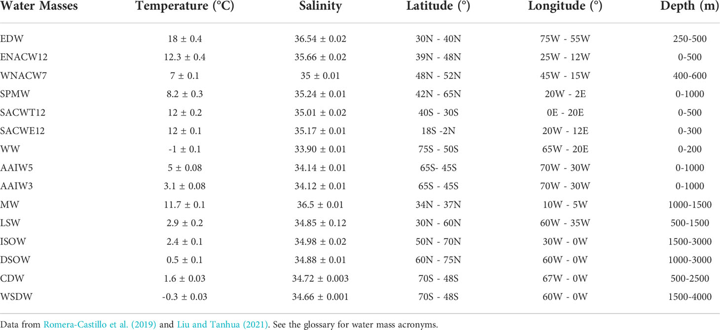
Table 1 Characteristics of the water masses used in this analysis in their respective formation areas, where they are considered to be pure (xij = 1).

Model analysis

In order to find good ML models for the water mass mixing problem, we trained ten multi-regression algorithms using the scikit-learn library (Pedregosa et al, 2011); namely, we studied the regression versions of K-Nearest Neighbors (K-NN) and decision trees, four variants of linear regression (classical, i.e. least squares linear regression; Lasso, i.e. linear regression trained with L1 prior as regularizer; ElasticNet, that is linear regression with combined L1 and L2 priors [AS1] [C2] [AS3] as regularizer; and Ridge regression), and four ensemble algorithms (extremely randomized trees, gradient boosting, random forest, and AdaBoost).

Due to the nature of our data, in particular to the fact that there are samples in the same location at different depths, and also due to the sort of models considered, we conducted a previous exhaustive analysis in order to avoid overfitting and data leakage.

Model selection, over-fitting and data leakage

Over-fitting is a frequent problem in regression models (Harrell, 2001) and it is usually due to bad quality of the data labeling, bias in the data collection or model characteristics. This issue arises when a model works properly with the training data, but it does not generalize to new data; fortunately, it can be detected by means of k-fold cross validation (Stone, 1974). This technique splits the dataset into k independent groups; and each of these groups is used to evaluate a model trained using the remaining groups. It is instrumental that the k groups are independent to assess the actual performance of the models. Another common problem that might arise with regression models is “data leakage” (Kaufman et al., 2012).

The original OMP database described in the previous section was split using 80% for training (9,011 samples, subset called train0) and 20% for testing (2,234 samples, subset called test0). To avoid data leakage, the split was performed taking into account that samples from the same location, even if they have been collected at different depths, can only belong to either the training or the testing set. In this way, the testing set is completely independent from the training set.

An additional split was necessary since we were interested in determining whether there is data leakage when both the training set and the testing set contain samples from the same location, but at different depths, and if this leads to over-fitting. To this aim, from train0 and test0, which do not share locations, we built two training sets (train1 and train2), and two testing sets (test1 and test2), see Figure 2. Train 1 is the same as train0, and test0 is divided into test1’ and test1. Therefore, the subsets train1 and test1 do not share instances with the same location. Now, test1’ is divided into test1’a and test1’b which do have samples with the same location. Train2 is then composed by joining train1 and train1’a and test2 is composed by test1’b and test1. Using these mixture sets, we achieve that train2 and test2 have samples with the same location (those shared by test1’a and test1’b). In addition, neither the pairs train1-test2 or train2-test1 share instances with the same locations. If data leakage is produced, the models trained using train2 would produce much better results when evaluated on test2 than when they are evaluated on test1.

FIGURE 2

Figure 2 Diagram of the strategy to obtain the training and testing sets to test over-fitting and data leakage.

Each training subset was employed to train several multi-regression algorithms with the scikit-learn library (Table 2). The algorithms were trained using the by-default hyper-parameters provided by the implementation of the scikit-learn library. A k-fold cross-validation (k=10) was used to select the model with each training subset and algorithm, and to detect over-fitting. Each fold of the cross-validation process was evaluated with R², being 1 the best possible score. The results were statistically analysed using a Friedman test to compare the R² means of each model since the parametricity conditions were not fulfilled. The algorithm that achieved the best performance was the extremely Randomized Trees Regression model (mean R²: 0.972991 and 0.963679 for train1 and train2, respectively), closely followed by the Random Forest Model (mean R²: 0.962375 and 0.940631 for train1 and train2, respectively). The rest of the models were far from such a performance (see Table 2). It is worth noting that the linear models failed to capture the relationship between the explanatory variables (features) and the percentages of water masses. The analysis of the Holm-Bonferroni method (Sheskin, 2011) gives that the Extremely Randomized Trees model is significantly different from all the other models except for K-NN, AdaBoost, and Random Forest Regressor. These results confirm that the best algorithm is Extremely Randomized Trees.

TABLE 2

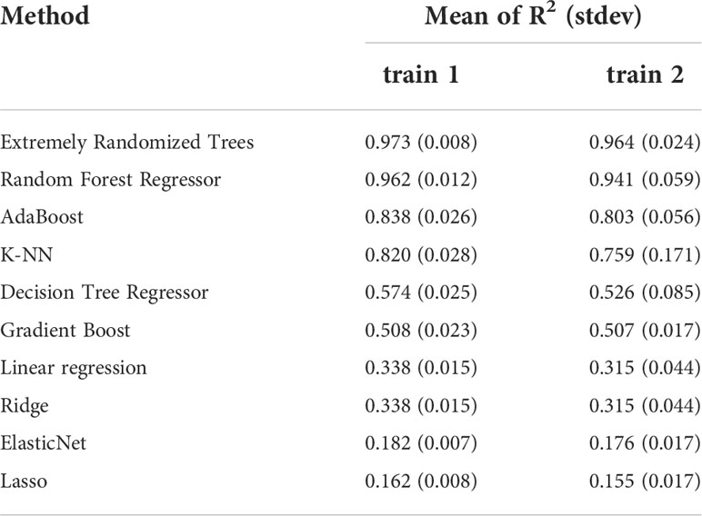
Table 2 Mean and standard deviation (in brackets) of R² score obtained from k-cross validation for each model and each dataset (train1 and train2) sorted in descending order.

For this model, we performed a further exploration of several combinations of their parameters and found that the best performance was obtained by using the default implementation of the scikit-learn library. Once the model with the best performance was selected, we checked whether there was over-fitting, since non-linear models, in particular decision trees, are known to be subject to over-fitting (Mitchell, 1997). To this aim, we built a model using the Extremely Randomized Trees algorithm for each training subset (train1 and train2). In order to detect and avoid over-fitting, each model was evaluated for each testing dataset obtaining the R² score summarized in Table 3.

TABLE 3

Table 3 R² score obtained from the trained models with both subsets of training and evaluated with both testing subset.

Please, note that in the ML models, water masses are not treated equally, without any weighting on their influence, but this difference is hidden in the training process and is due to the original OMP it is based on. Therefore, the different magnitudes of the contribution of each of the water masses are captured by the OMP and implicitly wired into the ML model during the training process.

From the obtained results, we can extract two lessons. First, there is no over-fitting nor data leakage in the model since the R² of the model train2-test2 (with repeated locations in both subsets) is lower than train2-test1 (without them). Second, without repeated locations in the training and testing datasets, the model generalizes slightly better.

All the experiments were conducted in an Intel(R) Core(TM) i7-4810MQ CPU at 2.80GHz, 16GB RAM.

Results

Features and results of the selected extremely randomized trees model

Once the best algorithm was selected (Extremely Randomized Trees), the model was built with the total training dataset (train0) and evaluated with the total testing dataset (test0). In this case, with no locations repeated in any dataset, the R² score obtained is 0.986902. Therefore, in the rest of this section we consider samples in the same location to be either in the training or testing data sets.

The relevance of each explanatory variable (feature) was also analysed using the Gini importance measure (Breiman, 2001) for the Extremely Randomized Trees regression model (Figure 3). This importance score provides a relative ranking of the employed features. In this model, the most relevant features were potential temperature and depth; whereas, longitude is the least relevant one.

FIGURE 3

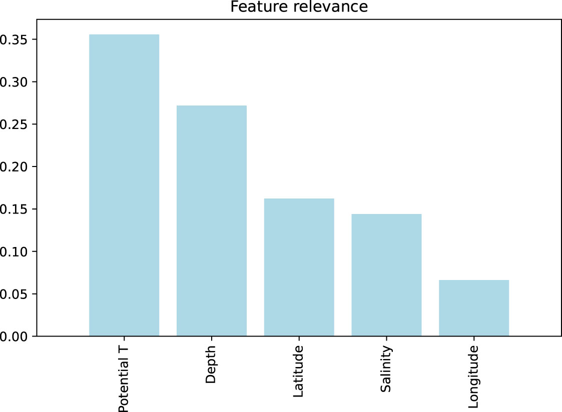
Figure 3 Feature relevance for the Extremely Randomized Trees regression model.

Addition of a pure water masses dataset to the existing model

In order to reinforce the model, we considered the impact of including the pure water masses dataset. First of all, the pure water masses dataset (2,920 data) was split using 60% for training and 40% for testing (again taking into account that samples from the same location only belong to either the training or the testing set), and the capacity of our model to be generalized to this dataset was analysed (Table 4). The performance of the model considerably decayed when evaluated in the new testing set (R² = 0.8482) formed only by samples from the pure water masses. This issue was handled by retraining the model with the new training data, i.e. adding samples from the pure water dataset to both the previous train and test OMP datasets. This approach solved the problem with the new data, improving the R² score to 0.9978 in the pure water masses dataset, and having a minimum impact in the OMP testing dataset (R² score only decayed by 0.0004). The R² score using the combined testing dataset was 0.9931. Therefore, even if the trained algorithm may fail when modeling out-of-distribution data, it can easily incorporate such data in a continual learning process (Liu, 2020). Observe that this is also an argument to discard over-fitting in our model.

TABLE 4

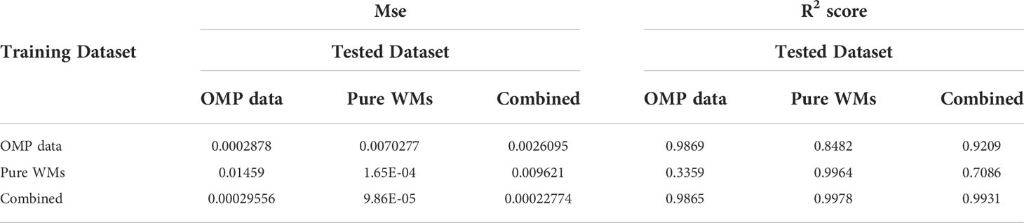
Table 4 Minimum square error (mse) and R² score of the Extremely Randomized Trees models when evaluated in the three testing sets: OMP dataset, pure WMs dataset, and combined OMP and pure WMs dataset for each of the trained dataset.

Addition of a new water mass to the existing model

Finally, we further analysed the robustness of the method by including a water mass that was not considered in the OMP used to initially train and test our model nor in the Pure Water Masses dataset. In our case we used the SAIW water mass whose characteristics are given in Table 5 according to Liu and Tanhua (2021). We collected the data from the GLODAPv2 database matching these characteristics and included them in the Pure Water Masses dataset.

TABLE 5

Table 5 Characteristics of the SAIW water mass.

Following the same methodology as in the previous analysis, we re-trained the Extremely Randomized Trees with the new dataset including samples from the SAIW water mass. As expected, the R² score decreased when the testing dataset is formed only by data from the OMP, since the SAIW water mass was not considered in that dataset; while the R² score improved for the Pure WMs test set and, more importantly, for the combined test data set (R²= 0.9945, Table 6). Notice that the R² in the model trained and tested with the OMP data is not exactly the one in Table 4, since we added a new water mass, which implies a new column in the OMP database with all values set to zero. This changed the model and the R² decreased from 0.9869 to 0.9727. This effect is much bigger when testing the Pure WMs set using a model trained with the OMP training set (and vice-versa), due to the presence of the nonzero values in the SAIW water mass columns of the Pure WMs datasets. The model trained combining both datasets does not, however, suffer this effect and maintains its good performance, showing the robustness of the method.

TABLE 6

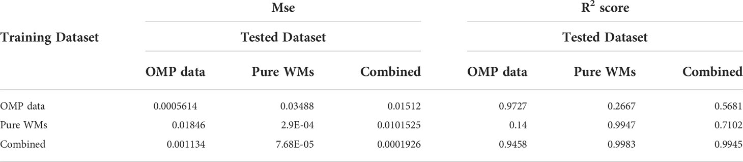
Table 6 Minimum square error (mse) and R² score of the Extremely Randomized Trees models when evaluated in the three testing sets including the SAIW water mass in the pure WMs dataset.

Finally, the feature relevance for the new model including the SAIW was analysed, obtaining similar results to those of the previous model (Figure 4).

FIGURE 4

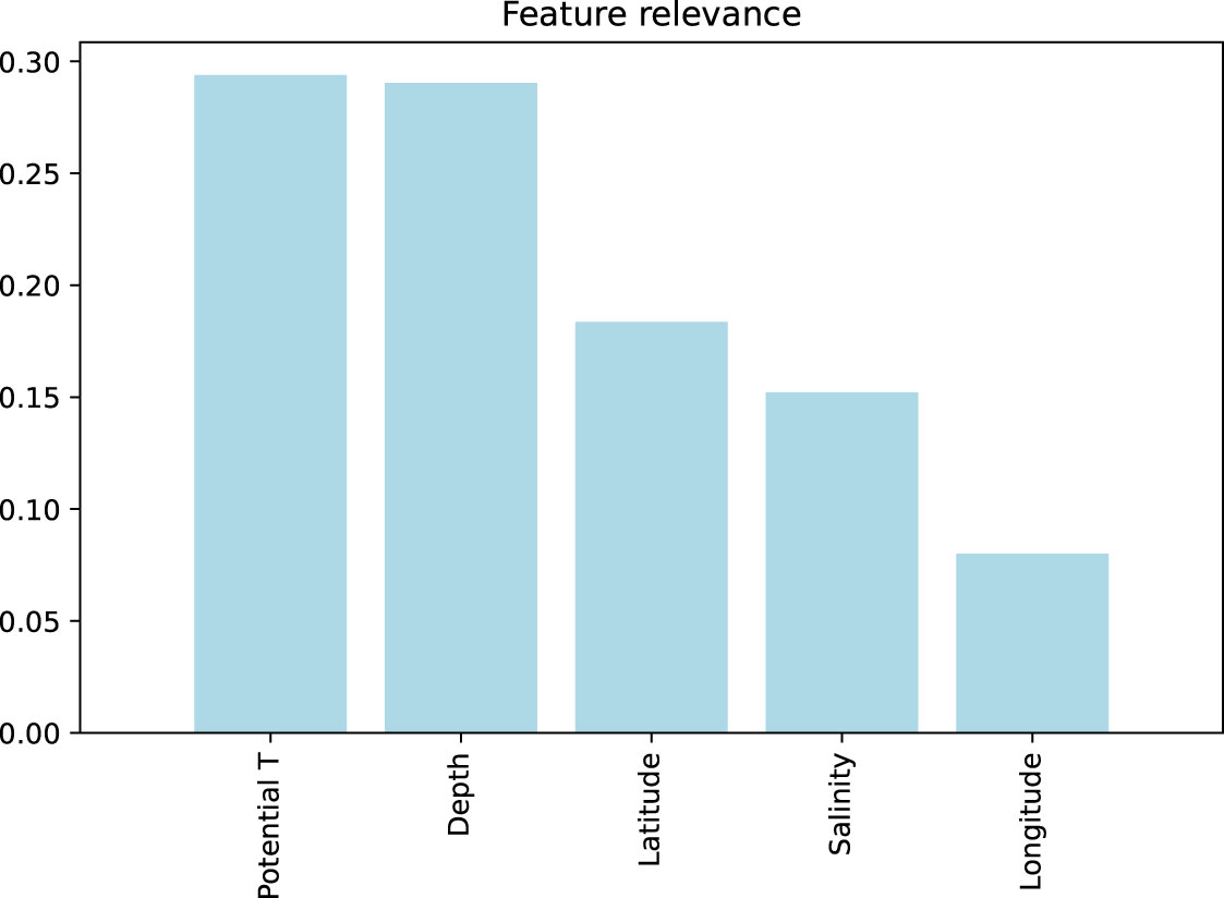
Figure 4 Feature relevance for the Extremely Randomized Trees regression model with the additional water mass SAIW.

Our validated model and the code can be downloaded from the Supplemental Information. The different models applied here and the data for developing our selected model are found in the folder "WaterMassMixing_models". Furthermore, we provide several scripts with different options to use our model on your own data. They are located in the folder "WaterMasses_inference". This material is also available online at the repositories github.com/joheras/WaterMassMixing and github.com/joheras/water-masses-inference.

Visualization of the extremely randomized trees model results

The water masses contribution to each sample obtained with our algorithm was plotted for two transects included in the OMP training dataset: A16 (Figure 5) and A22 (Figure 6), as well as for another three ones not included: A9.5 (Figure 7), A25 (Figure 8) and A03 (Figure 9). As expected, according to the low mse and high R² between the results of the algorithm and those from the OMP analysis, the distribution of the water masses agrees with that obtained with the OMP analysis for the A16 section (Romera-Castillo et al., 2019). Also, the water masses in the rest of the sections agree with previous works (e.g., Liu and Tanhua, 2021; Talley et al., 2011) including the sections not used in the OMP training dataset (A9.5, A25 and A03). Central water masses (ENACW₁₂, SACWT₁₂, EDW) covered the upper water column from 250m until 800 m for ENACW₁₂, 600 m for SACWT₁₂ and 400 m for EDW close to the Caribbean and to 700 m in the Sargasso Sea. At intermediate levels, AAIW was centered at 800 m while LSW core flow ranged between 1500 and 2000 m. SPMW descended in depth along the A25 section from < 250 m near Greenland to around 1000 m near the Iberian Peninsula. It is also visible in the A03 section from 45°W to the east, centered at 1000 m. MW was centered at 1000 m and its fraction did not exceed the 50% in any of the sections. SAIW, which was not included in the OMP dataset and was obtained from the model, was very low represented in the A03 section with less than 0.02% of contribution in the middle of the section from surface to 2000 m, while it was more abundant in the A25 section, close to Greenland, and decreased to the southeast (Figure 10). Bashmachnikov et al. (2015) showed a contribution of up to 50% of the SAIW along the 40°N, located north than ours. The difference between their results and ours, in which we found a lower contribution than them, is likely due to the difference source water type characteristics that they considered for the SAIW.

FIGURE 5

Figure 5 A16 section for the contribution of the water masses (A) AAIW5, (B) ENACW12, (C) AAIW3, (D) MW, (E) LSW, (F) ISOW, (G) CDW and (H) WSDW. Figure with the Ocean Data View software (Schlitzer, 2015).

FIGURE 6

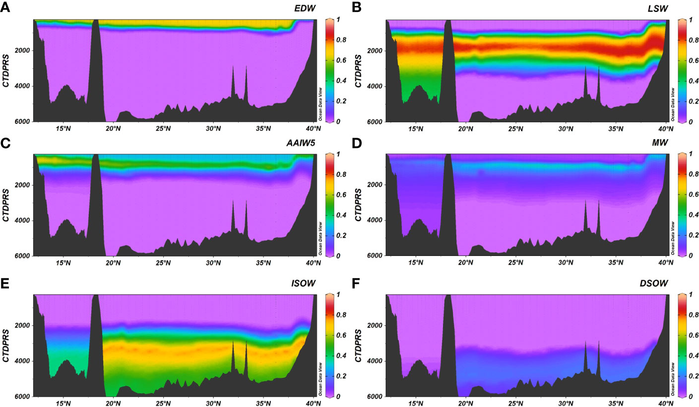
Figure 6 A22 section for the contribution of the water masses (A) EDW, (B) LSW, (C) AAIW5, (D) MW, (E) ISOW, (F) DSOW. Figure with the Ocean Data View software (Schlitzer, 2015).

FIGURE 7

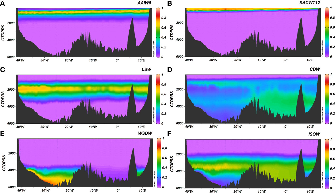
Figure 7 A9.5 section for the contribution of the water masses (A) AAIW5, (B) SACWT12, (C) LSW, (D) CDW, (E) WSDW, (F) ISOW. Figure with the Ocean Data View software (Schlitzer, 2015).

FIGURE 8

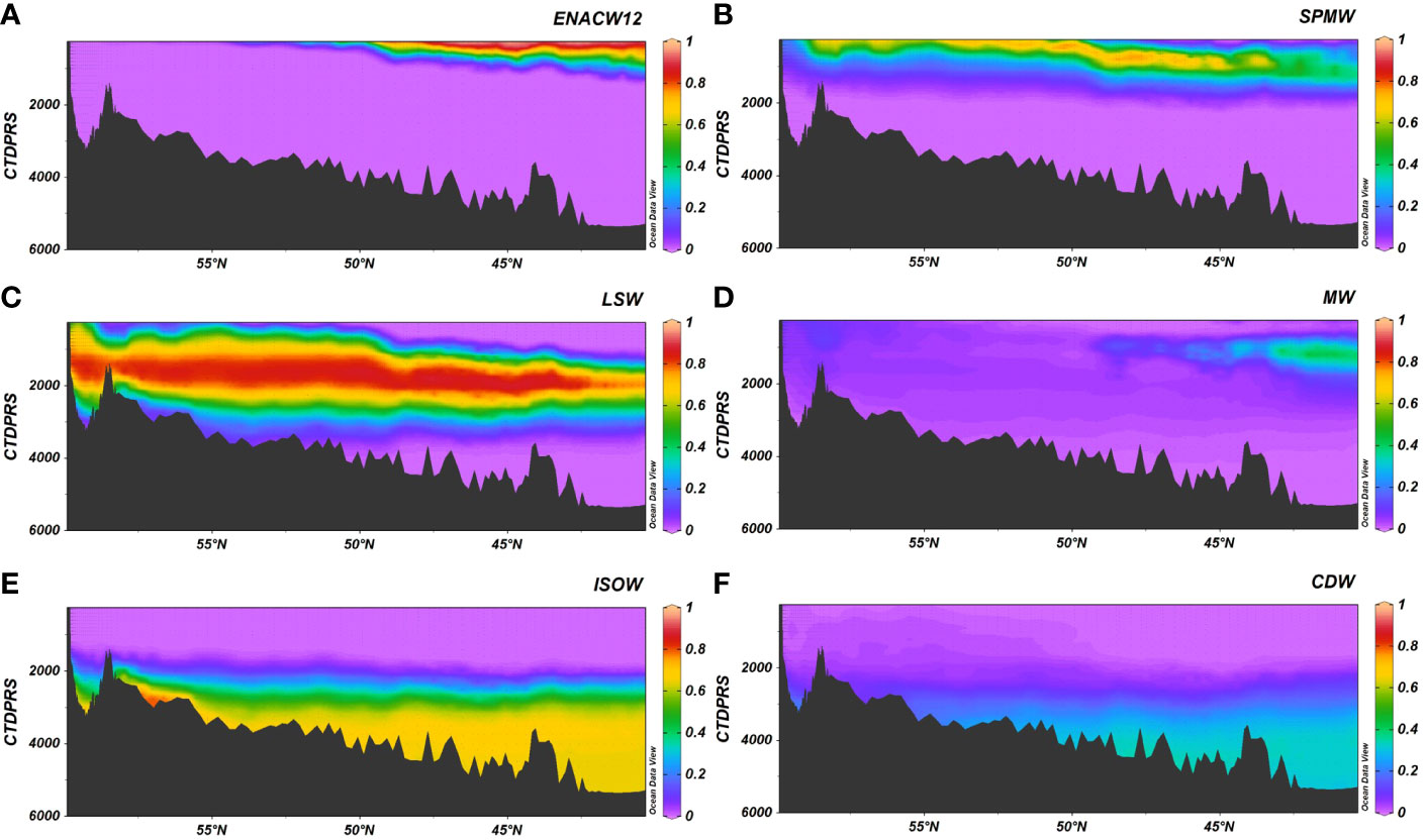
Figure 8 A25 section for the contribution of the water masses (A) ENACW12, (B) SPMW, (C) LSW, (D) MW, (E) ISOW, (F) CDW. Figure with the Ocean Data View software (Schlitzer, 2015).

FIGURE 9

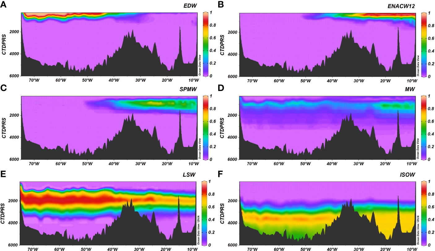
Figure 9 A03 section for the contribution of the water masses (A) EDW, (B) ENACW12, (C) SPMW, (D) MW, (E) LSW, (F) ISOW. Figure with the Ocean Data View software (Schlitzer, 2015).

FIGURE 10

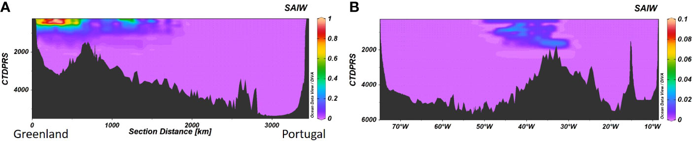
Figure 10 SAIW contribution for the (A) A25 and (B) A03 sections. Note the different scale in Figure 2B.

Deep waters occupied the bottom part of the water column with ISOW spreading below 3000 m up to 30°S and WSDW covering the South Atlantic up to the Equator. DSOW was present below 3000 m in very low proportion (< 1%) from close to Massachusetts coast to 19°N along A22 section. CDW sunk in the South Atlantic Ocean and split in two branches on its way to the north along the A16 section, being detected in the water column from 1000 to the bottom. It arrived to the 24°S (A9.5 section) with a fraction lower than 50% (Figure 7) and it is still recognizable until 54°N below 3500 m with a contribution of 30% (Figure 5). Note that North Atlantic Deep Water (NADW) typically encountered in the Eastern North Atlantic is decomposed into ISOW, DSOW, CDW and WSDW.

Discussion

We have proven that Machine Learning techniques provide tools for the study of water mass mixing in the ocean based on potential temperature, salinity, position and depth of the water samples. We have performed an analysis of samples in several cruises using different algorithms. Among these, we found that the Extremely Randomized Trees (Geurts et al., 2006) is the most suitable. The Extremely Randomized Trees is a supervised machine learning algorithm that can be used for both regression and classification tasks, and that has been widely applied to tackle different problems. It consists of an ensemble of decision trees and it is related to other similar algorithms such as bootstrap aggregation and random forests, widely used in ML. This algorithm creates a large set of decision trees from the training dataset and, in the case of the regression version, which is the one used here, acts by averaging the prediction of the decision trees. It is a method that features both accuracy and computational efficiency. In engineering, the Extremely Randomized Trees algorithm has been used to predict the energy consumption of buildings (Gong et al., 2020), performance for bioenergy crop modeling (Huntington et al, 2020), or to estimate wind farm power production based on atmospheric turbulences (Optis and Perr-Sauer, 2019). This algorithm has been also applied in Earth sciences, in Geology, to estimate pre‐eruptive temperatures and storage depths on volcanoes (Petrelli et al., 2020) or to explore the link between microseisms and sea ice (Cannata et al., 2019). In the aquatic sciences context, this algorithm has been employed to automatically map mangroves (Bunting et al., 2018), to classify plankton on images (Ellen et al., 2019) or to model daily lake surface water temperature from air temperature (Heddam et al., 2020). However, the potential of this algorithm had not been yet exploited in Oceanography, being their applications reduced to a few marine science problems such as the determination of bathymetry, bottom type, and water column optical properties from hyperspectral imagery (Nock et al., 2019) or to classify seamounts derived from bathymetry data (Lawson et al., 2017).

Furthermore, the application of ML algorithms does not assume any particular form of mathematical relation between the variables. OMP methods assume linear dependence between the variables and impose a limitation on the number of water masses contributing to a given sample, due to the limitation in the number of variables (Tomczak, 1981). On the other side, nonlinear methods applied in the literature, such as in De La Fuente et al. (2017), do not give the proportions of the water masses, which is one of the objectives sought here. Even if the method in De La Fuente et al. (2017) assumes polynomial dependence among the variables and does not have a limitation on the number of water masses involved, it has, however, the limitations inherent to any regression model, in particular, its accuracy depends on the number of available samples, and one needs to decide on a priori relationship between the variables involved (e.g. a particular quadratic or cubical polynomial).

Advantages and applications of our approach

The application of our ML approach to ocean water masses identification and quantification has three main advantages regarding previous methodologies. The first one is that our method, other than position and depth, only needs two characteristic variables, namely potential temperature and salinity, which are the core conservative variables more commonly collected and curated in oceanography both from oceanographic cruises and autonomous vehicles (Boyer et al., 2018; Olsen et al., 2020; ARGO). Our ML avoids the need of using less commonly measured chemical variables and which require longer and time consuming analyses of both the water samples and the data.

A second advantage is that previously used methods also require an extensive knowledge of the oceanography of the studied area, the Atlantic Ocean in our case. But our approach will bring a wider range of marine scientists, non-particularly expert in hydrography, to the resolution of water mass mixing. This will allow marine scientists to go further in the understanding of the biogeochemical processes affecting the variation of chemical and biological variables.

Finally, a third advantage of this approach is the possibility to coherently integrate data from different studies. The proposed methodology can take advantage of previous knowledge about water mass mixing in the ocean and can analyse new data using earlier work. For instance, the data used in Section 2 applied the OMP analysis from Romera-Castillo et al. (2019) and added information about pure water masses from different geographical zones, thus covering particular areas of the Atlantic Ocean. As we observed, the newly introduced data did not significantly affect the accuracy of the model on the original data set while, at the same time, the accuracy of the predictions improved significantly on the new data. Additional OMP databases obtained using the same source water type characteristics than used here could be added to further train the model by coherently incorporating their results. We have also proven that the model can be fed with a new water mass but the accuracy is higher if it is included in the training model from the beginning. Also, note that if other source water types want to be defined, then a new model should be trained with the new pure WMs database and the corresponding OMP obtained with them. Otherwise, the analysis of new samples using our model will be assuming the source water types characteristics given here. Note that using the trained model, the number of new samples to be analysed is no longer important, even a single sample could be analysed and the precision would be that of the full model. Our model can be downloaded and the user can easily introduce the required variables (latitude, longitude, depth, temperature and salinity) of the chosen Atlantic samples and obtain the WM proportion of each one in a fast and easy way. Actually, it would allow the user to obtain this information in real time during a cruise. Therefore, this will be a useful tool for anyone interested on the subject.

In summary, using the proposed methodology, researchers can take advantage of previous knowledge validated by the community to solve the problem of water masses composition in the Atlantic Ocean for any number of samples by just considering the location, depth, potential temperature and salinity of such samples. New research using other methods like OMP and its variants can be incorporated to the existing model increasing its accuracy and prediction capacity.

Data availability statement

The original contributions presented in the study are included in the article/Supplementary Materials. Further inquiries can be directed to the corresponding author.

Author contributions

CR-C and ES-d-C had the original idea, designed the research and coordinated the group. JH, GM and ES-d-C implemented and run the algorithms. All the authors contributed to the interpretation of the data and the discussion of the results presented in the manuscript. CR-C wrote the first draft of the manuscript and all the authors made comments and amendments, and approved the final version.

Funding

CR-C was funded by grant PID2019-109889RJ-I00 / AEI / 10.13039/501100011033 (Ministerio de Ciencia e Innovación and Agencia Estatal de Investigación, Spain). GM and JH were partially supported by Ministerio de Ciencia e Innovación [PID2020-115225RB-I00 / AEI / 10.13039/501100011033]. ES-d-C was partially supported by Ministerio de Ciencia e Innovación [PID2020-116641GB-100 / AEI / 10.13039/501100011033]. XA–S was partially funded by grant number PID2019-109084RB-C22 (Ministerio de Ciencia e Innovación, Spain). MA was funded by RADPROF and RADIALES IEO-CSIC projects.

Acknowledgments

We acknowledge the “Severo Ochoa Centre of Excellence” accreditation (CEX2019-000928-S).

Conflict of interest

The authors declare that the research was conducted in the absence of any commercial or financial relationships that could be construed as a potential conflict of interest.

Publisher’s note

All claims expressed in this article are solely those of the authors and do not necessarily represent those of their affiliated organizations, or those of the publisher, the editors and the reviewers. Any product that may be evaluated in this article, or claim that may be made by its manufacturer, is not guaranteed or endorsed by the publisher.

Supplementary material

The Supplementary Material for this article can be found online at: https://www.frontiersin.org/articles/10.3389/fmars.2022.904492/full#supplementary-material

Abbreviations

DOC, dissolved organic carbon; K-NN, K-Nearest Neighbours; ML, machine learning; OMP, optimum multiparametric analysis; EDW, Eighteen Degrees Water; ENACW, Eastern North Atlantic Central Water of 12°C; WNACW, Western North Atlantic Central Water of 7°C; SPMW, Subpolar Mode Water; SACW-T₁₂, Subtropical South Atlantic Central Water of 12°C; SACW-E, Equatorial South Atlantic Central Water of 12° C; SAIW, Subarctic Intermediate Water; WW, Winter Water; AAIW, Antarctic Intermediate Water of 5°C (Subantarctic Mode Water); AAIW, Antarctic Intermediate Water of 3°C; MW, Mediterranean Water; LSW, Labrador Sea Water; ISOW, Iceland-Scotland Overflow Water; DSOW, Denmark Strait Overflow Water; CDW, Circumpolar Deep Water; WSDW, Weddell Sea Deep Water; WM, Water Mass.

References

Ahmad H. (2019). Machine learning applications in oceanography. Aquat. Res. 2 (3), 161–169. doi: 10.3153/AR19014

CrossRef Full Text | Google Scholar

Álvarez M., Brea S., Mercier H., Álvarez-Salgado X. A. (2014). Mineralization of biogenic materials in the water masses of the south Atlantic ocean. I: Assessment and results of an optimum multiparameter analysis. Prog. Oceanogr. 123 (0), 1–23. doi: 10.1016/j.pocean.2013.12.007

CrossRef Full Text | Google Scholar

Álvarez-Salgado X. A., Álvarez M., Brea S., Mèmery L., Messias M. J. (2014). Mineralization of biogenic materials in the water masses of the south Atlantic ocean. II: Stoichiometric ratios and mineralization rates. Prog. Oceanogr. 123 (0), 24–37. doi: 10.1016/j.pocean.2013.12.009

CrossRef Full Text | Google Scholar

ARGO. Available at: https://argo.ucsd.eduhttps://www.ocean-ops.org.

Google Scholar

Bashmachnikov I., Nascimento Â., Neves F., Menezes T. (2015). Distribution of intermediate water masses in the subtropical northeast Atlantic. Ocean Sci. Discuss 12, 769–822. doi: 10.5194/osd-12-769-2015

CrossRef Full Text | Google Scholar

Bittig H. C., Steinhoff T., Claustre H., Fiedler B., Williams N. L., Sauzède R., et al. (2018). An alternative to static climatologies: Robust estimation of open ocean CO2 variables and nutrient concentrations from T, s, and O2 data using Bayesian neural networks. Front. Mar. Sci. 5 (328). doi: 10.3389/fmars.2018.00328

CrossRef Full Text | Google Scholar

Boyer T. P., Baranova O. K., Coleman C., Garcia H. E., Grodsky A., Locarnini R. A., et al. (2018). World ocean database 2018 Vol. 87. Ed. Mishonov A. V. (NOAA Atlas NESDIS). Silver Spring, MD. Available at: https://www.ncei.noaa.gov/sites/default/files/2020-04/wod_intro_0.pdf.

Google Scholar

Breiman L. (2001). Random forests. Mach. Learn. 45, 5–32. doi: 10.1023/A:1010933404324

CrossRef Full Text | Google Scholar

Bunting P., Rosenqvist A., Lucas R. M., Rebelo L.-M., Hilarides L., Thomas N., et al. (2018). The global mangrove watch–a new 2010 global baseline of mangrove extent. Remote Sens. 10, 1669. doi: 10.3390/rs10101669

CrossRef Full Text | Google Scholar

Cannata A., Cannavò F., Moschella S., Gresta S., Spina L. (2019). Exploring the link between microseism and sea ice in Antarctica by using machine learning. Sci. Rep. 9 (1), 13050. doi: 10.1038/s41598-019-49586-z

PubMed Abstract | CrossRef Full Text | Google Scholar

Claustre H., Johnsson K., Biogeochemical-Argo Planning Group (2016). The scientific rationale, design and implementation plan for a biogeochemical-argo float array. doi: 10.13155/46601

PubMed Abstract | CrossRef Full Text | Google Scholar

D’Alelio D., Rampone S., Cusano L. M., Morfino V., Russo L., Sanseverino N., et al. (2020). Machine learning identifies a strong association between warming and reduced primary productivity in an oligotrophic ocean gyre. Sci. Rep. 10, 3287. doi: 10.1038/s41598-020-59989-y

PubMed Abstract | CrossRef Full Text | Google Scholar

De la Fuente P., Pelegrí J. L., Canepa A., Gasser M., Domínguez F., Marrasé C., et al. (2017). And end-Member-Free approach for obtaining ocean remineralization patterns. J. Atmos. Oceanic Technol. 34, 2443–2455. doi: 10.1175/JTECH-D-17-0090.1

CrossRef Full Text | Google Scholar

Ellen J. S., Graff C. A., Ohman M. D. (2019). Improving plankton image classification using context metadata. Limnol Oceanogr. Methods 17, 439–461. doi: 10.1002/lom3.10324

CrossRef Full Text | Google Scholar

Geurts P., Ernst D., Wehenkel L. (2006). Extremely randomized trees. Mach. Learn 63, 3–42. doi: 10.1007/s10994-006-6226-1

CrossRef Full Text | Google Scholar

Gong M., Wang J., Bai Y., Li B., Zhang L. (2020). Heat load prediction of residential buildings based on discrete wavelet transform and tree-based ensemble learning. J. Build. Eng. 32, 101455. doi: 10.1016/j.jobe.2020.101455

CrossRef Full Text | Google Scholar

Harrell F. E. Jr. (2001). Regression modeling strategies (London: Springer).

Google Scholar

Heddam S., Ptak M., Zhu S. (2020). Modelling of daily lake surface water temperature from air temperature: Extremely randomized trees (ERT) versus Air2Water, MARS, M5Tree, RF and MLPNN. J. Hidrology 588, 125130. doi: 10.1016/j.jhydrol.2020.125130

CrossRef Full Text | Google Scholar

Huntington T., Cui X., Mishra U., Scown C. D. (2020). Machine learning to predict biomass sorghum yields under future climate scenarios. Biofuels Bioproducts Bior. 14 (3), 566–577. doi: 10.1002/bbb.2087

CrossRef Full Text | Google Scholar

Kaufman S., Rosset S., Perlich C. (2012). Leakage in data mining: Formulation, detection, and avoidance. ACM Trans. Knowl. Discovery Data 6 (4), 1–21. doi: 10.1145/2382577.2382579

CrossRef Full Text | Google Scholar

Lawson E., Smith D., Sofge D., Elmore P., Petry F. (2017). Decision forests for machine learning classification of large, noisy seafloor feature sets. Comput. Geosciences 99, 116–124. doi: 10.1016/j.cageo.2016.10.013

CrossRef Full Text | Google Scholar

Liu B. (2020). Learning on the job: Online lifelong and continual learning. Proc. AAAI Conf. Artif. Intell. 34 (09), 13544–13549. doi: 10.1609/aaai.v34i09.7079

CrossRef Full Text | Google Scholar

Liu M., Tanhua T. (2021). Water masses in the Atlantic ocean: characteristics and distributions. Ocean Sci. 17, 463–486. doi: 10.5194/os-17-463-2021

CrossRef Full Text | Google Scholar

Mitchell T. M. (1997). Machine learning (New York, NY, USA: McGraw-Hill).

Google Scholar

Nock K., Gilmour E., Elmore P., Leadbetter E., Sweeney N., Petry F. (2019). Deep learning on hyperspectral data to obtain water properties and bottom depths. Signal Process Sensor/Information Fusion Target Recognit. XXVIII 11018, 110180Y. doi: 10.1117/12.2519881

CrossRef Full Text | Google Scholar

Olsen A., Lange N., Key R. M., Tanhua T., Bittig H. C., Kozyr A., et al. (2020). An updated version of the global interior ocean biogeochemical data product, GLODAPv2.2020, earth syst. Sci. Data 12, 3653–3678. doi: 10.5194/essd-12-3653-2020

CrossRef Full Text | Google Scholar

Optis M., Perr-Sauer J. (2019). The importance of atmospheric turbulence and stability in machine-learning models of wind farm power production. Renewable Sustain. Energy Rev. 112, 27–41. doi: 10.1016/j.rser.2019.05.031

CrossRef Full Text | Google Scholar

Pardo P. C., Pérez F. F., Velo A., Gilcoto M. (2012). Water masses distribution in the southern ocean: Improvement of an extended OMP (eOMP) analysis. Prog. In Oceanogr. 103 (0), 92–105. doi: 10.1016/j.pocean.2012.06.002

CrossRef Full Text | Google Scholar

Pedregosa F., Varoquaux G., Gramfort A., Michel V., Thirion B., Grisel O., et al. (2011). Scikit-learn: Machine learning in Python. JMLR 12, 2825–2830. doi: 10.5555/1953048.2078195

CrossRef Full Text | Google Scholar

Petrelli M., Caricchi L., Perugini D. (2020). Machine learning thermo-barometry: Application to clinopyroxene-bearing magmas. JGR Solid Earth 125, e2020JB020130. doi: 10.1029/2020JB020130

CrossRef Full Text | Google Scholar

Poole R., Tomczak M. (1999). Optimum multiparameter analysis of the water mass structure in the Atlantic ocean thermocline, deep Sea research part I. Oceanogr. Res. Papers 46, 1895–1921. doi: 10.1016/S0967-0637(99)00025-4

CrossRef Full Text | Google Scholar

Reinthaler T., Álvarez-Salgado X. A., Álvarez M., van Aken H. M., Herndl G. J. (2013). Impact of water mass mixing on mineralization and biogeochemistry in the north Atlantic deep water. Global Biogeochem. Cycles 27, 1151–1162. doi: 10.1002/2013GB004634

PubMed Abstract | CrossRef Full Text | Google Scholar

Romera-Castillo C., Álvarez M., Pelegrí J. L., Hansell D. A., Álvarez-Salgado X. A. (2019). Net additions of recalcitrant dissolved organic carbon in the deep Atlantic ocean. Global Biogeochem. Cycles 33, 1162–1173. doi: 10.1029/2018GB006162

CrossRef Full Text | Google Scholar

Schlitzer R. (2015) Ocean data view. Available at: https://odv.awi.de (Accessed 2017).

Google Scholar

Sheskin D. (2011). Handbook of parametric and nonparametric statistical procedures (London: CRC Press).

Google Scholar

Stone M. (1974). Cross-validatory choice and assessment of statistical predictions. J. R. Stat. Society. Ser. B (Methodological) 36 (2), 111–147. doi: 10.1111/j.2517-6161.1974.tb00994.x

CrossRef Full Text | Google Scholar

Talley L. D., Pickard G. L., Emery W. J., Swift J. H. (2011). Descriptive physical oceanography. Sixth Edition (Londong: Academic Press), 245–301.

Google Scholar

Tomczak M. (1981). A multi-parameter extension of temperature/salinity diagram techniques for the analysis of non-isopycnal mixing. Prog. Oceanogr. 10, 147–171. doi: 10.1016/0079-6611(81)90010-0

CrossRef Full Text | Google Scholar