
94% of researchers rate our articles as excellent or good
Learn more about the work of our research integrity team to safeguard the quality of each article we publish.
Find out more
ORIGINAL RESEARCH article
Front. Mar. Sci. , 22 August 2022
Sec. Marine Fisheries, Aquaculture and Living Resources
Volume 9 - 2022 | https://doi.org/10.3389/fmars.2022.903035
 Fiona Bairstow1
 Sven Gastauer2,3
 Simon Wotherspoon4
 C. Tom A. Brown1
 So Kawaguchi4
 Tom Edwards1
 Martin J. Cox4*
Krill are the subject of growing commercial fisheries and therefore fisheries management is necessary to ensure long-term sustainability. Krill catch limits, set by Commission for the Conservation of Antarctic Marine Living Resources, are based on absolute krill biomass, estimated from acoustic-trawl surveys. In this work, we develop a method for determining an error budget for acoustic-trawl surveys of krill which includes sampling and measurement variability. We use our error budget method to examine the sensitivity of biomass estimates to parameters in acoustic target strength (TS) models, length frequency distribution and length to wetmass relationships derived from net data. We determined that the average coefficient of variation (CV) of estimated biomass was 17.7% and the average CV due from scaling acoustic observations to biomass density was 5.3%. We found that a large proportion of the variability of biomass estimates is due to the krill orientation distribution, a parameter in the TS model. Orientation distributions with narrow standard deviations were found to emphasise the results of nulls in the TS to length relationship, which has to potential to lead to biologically implausible results.
Antarctic krill (Euphausia superba) are an intrinsic component of the Antarctic ecosystem, through which a large proportion of energy and nutrients of the antarctic system flow (Mauchline and Fisher, 1969; Everson, 1977; Kock, 1985; Howard, 1989). Krill are relied upon as a food source for a variety of Antarctic wildlife including seals, penguins, whales and sea birds (Kock, 1985; Trathan and Hill, 2016; Nicol, 2018). Commercial fisheries also target krill, which can be sold as fish food for aquariums and aquaculture (Kawaguchi and Nicol, 2020). The long-term sustainability of these fishing practices is managed through precautionary catch limits set by the Commission for the Conservation of Antarctic Marine Living Resources (CCAMLR). Krill biomass is a key parameter used to calculate krill catch limits (Constable and De la Mare, 1996). In this work we have used Antarctic krill as an example to assess the accuracy and sensitivity of biomass estimates arising from acoustic-trawl surveys.
Biomass estimates of marine resources are essential for fisheries management, the monitoring of environmental impact, and to improve our understanding of ecology. Due to their wide geographical distribution, the biomass of pelagic species that aggregate, e.g. herring and krill, are commonly estimated from acoustic-trawl surveys. Here, we develop an error budget for krill biomass surveys that brings together recent work in krill target strength (Bairstow et al., 2021) and geostatistical techniques [e.g. Maravelias et al. (1996); Woillez et al. (2009)] to provide biomass estimates that include sampling and measurement errors (stochastic error).
The acoustic component of the survey is carried out to map the marine resource using calibrated echosounders (Demer et al., 2015) that are typically vessel mounted (e.g. Reiss et al., 2008). Compared to net data, acoustic data is sampled rapidly along transects and to depths of several 100 metres (250 metres for krill). Acoustics, however, have an important limitation: it is not currently possible to transform acoustic echoes arising from the species of interest, in this case krill, directly to biomass density without additional biological information, which is typically obtained by net sampling.
Without samples from nets, or cameras, we cannot determine if an echo observed in a given volume, measured as volume backscattering coefficient (sv; units: m -1) arises from, in extreme cases, a few large animals, or a tightly packed group of many small animals. The acoustic density attributed to krill echos sA (Nautical Area Scattering Coefficient; units: m2nmi-2) is the integral of sv over a range interval multiplied by a constant (MacLennan et al., 2002). The scaling of sA to biomass density is carried out using the backscattering cross section (σbs; units: m2), the linear form of the acoustic target strength (TS; units: dB re 1 m2). TS depends on a variety of factors including: acoustic frequency, target size, shape, material properties and orientation (Calise and Skaret, 2011; Bairstow et al., 2021). The echosounder frequency must be carefully selected to maximise range in sea water while maintaining sensitivity to the species of interest.
Net samples are used to estimate the krill length to wetmass relationship and distributions of length and shape, e.g. radius, (Figure 1). The length and shape distributions are then used to model survey-specific krill TS. Following Hewitt and Demer (2000) both krill wetmass and krill TS relationships are typically parameterised with respect to length (W(l) and TS(l) respectively.) Acoustic observations (sA) are scaled to areal animal biomass density (gm-2) using the survey-specific krill TS and wetmass relationships (see section 2.3).
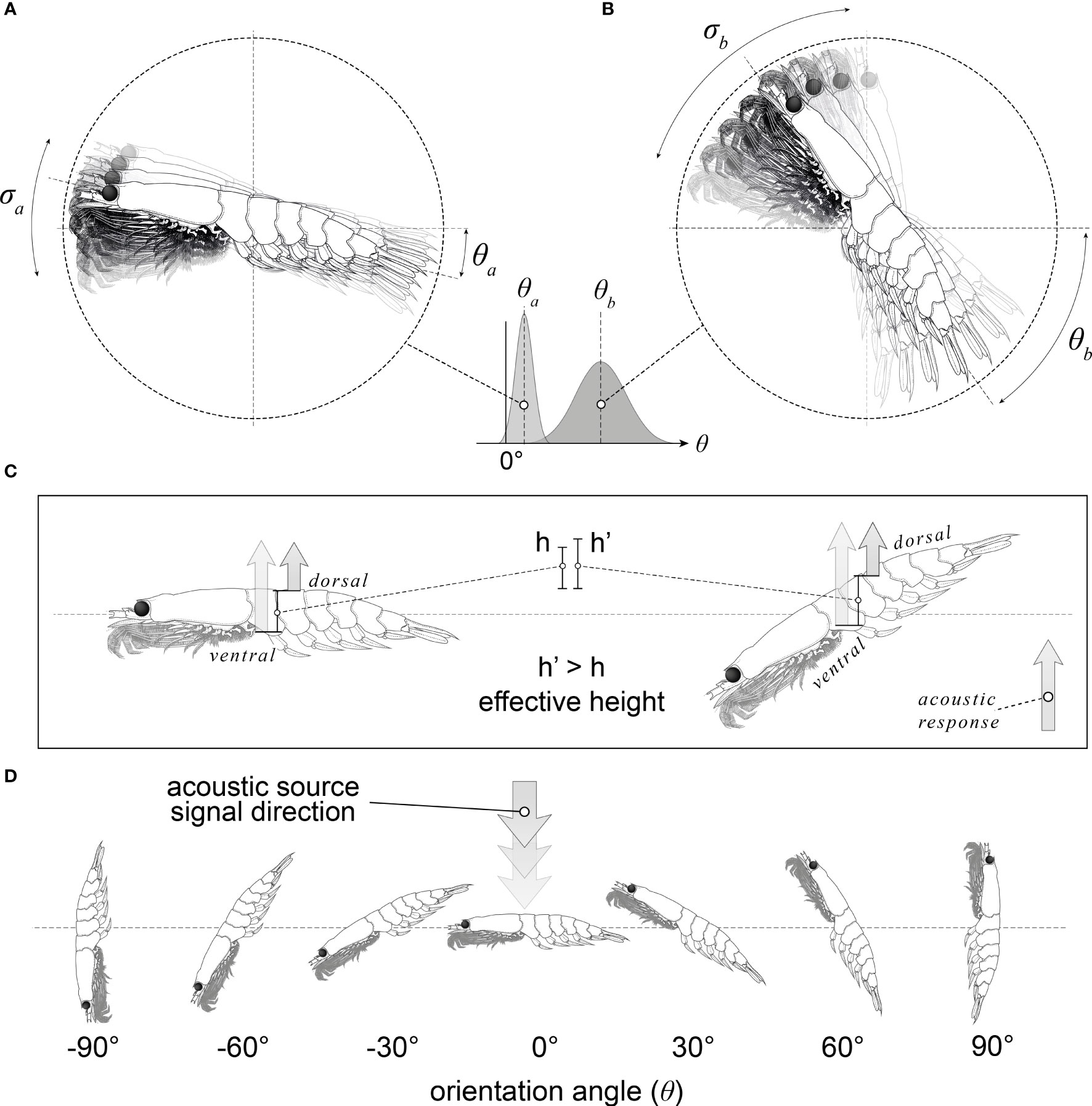
Figure 1 An illustration of krill orientation with respect to the incident acoustic beam. Panels (A, B) illustrate the range of krill orientations present within a swarm of krill; a: low mean orientation (ϴa) and small standard deviation (aa), b: high mean orientation (ϴb) and large standard deviation (σa). A krill orientation distribution is approximated as a Gaussian distribution with a mean orientation angle and a standard deviation. Panel (C) depicts how the orientation of the krill changes the effective height (the distance between the dorsal and ventral surfaces in the direction of the incident acoustic wave). Panel (D) depicts a range of krill orientations where to orientation angle is the angle between the incident acoustic beam and a normal to the midline of the krill.
Another component of TS estimation is orientation angle distribution, which cannot be directly observed from nets or conventional continuous wave acoustic observations for krill. Orientation angle is defined as the angle between the incident acoustic beam and a normal to the mid-line of the target as depicted in Figure 1. In situ observations of orientation are complex to observe (Kubilius et al., 2015), and in the case of Antarctic krill, there is currently no agreed upon method for doing so alongside acoustic-trawl surveys.
Measurements of acoustic density attributed to krill echoes sA across a survey domain are spatially dependent. Therefore, to model sA at all locations within a survey domain requires careful consideration of this spatial dependence (Petitgas, 1993). The use of geostatistics (Matheron, 1971) is widely regarded as an appropriate method for estimating the abundance and sampling errors of fish populations from acoustic-trawl surveys (Petitgas, 2001).
Geostatistical Conditional Simulations (GCS) are particularly powerful when it comes to combining data from a range of sources and representing the spatial variability of a given variable (Woillez et al., 2009; Gastauer et al., 2017). GCS have previously been used to calculate the distribution, density and relative abundances of krill or other pelagic species (Simard et al., 2003; Woillez et al., 2009). This method allows us to produce multiple simulations of the population structure while honouring the data. Coefficients of variation (CV) representing the sampling error are then calculated.
Beyond sampling variability, krill biomass estimates do not typically include an error budget [but see Demer (2004)]. The components of biomass estimation, such as the relationship between length and wetmass, and length and TS are neglected when calculating biomass errors. In this study, we develop a total error budget of a krill biomass estimate by combining spatial variation (sampling variability) and observational errors.
The overall objective of this work is to develop a method to calculate an error budget for biomass estimates of pelagic species that can be sampled using acoustics and nets. We use data from ship-based acoustic-trawl surveys of krill to illustrate a simulation based approach for estimating biomass error budgets. This approach can also be applied to surveys of other pelagic species and extended to include additional data sets should they be available.
Biomass estimation requires the systematic or random sampling of a species of interest within a finite domain or survey area, Asurvey.
The following sections describe the acoustic data and catch data collected during acoustic trawl surveys. These sections are followed by an explanation of the use of this data to estimate biomass.
We considered active acoustic data and catch data i.e. TS, length, ratio of length to radius, and wetmass. Additional shape data, described in Bairstow et al. (2021), was also considered. As the purpose of this research is to develop and illustrate methods for biomass estimation, we used data collected during three voyages:
At the time of writing, we did not have access to a complete set of krill survey data which could be used to investigate sampling and measurement variability. By using different data-types collected during three surveys we did, however, have sufficient data for our investigation. Using a combination of data from three different surveys of krill is a reasonable approach since the purpose of our research was not to estimate a krill biomass per se, rather we are developing methods that can be used to estimate krill density.
The first source of data was the Euphausiids and Nutrient Recycling In Cetacean Hotspots, ENRICH, voyage in the East Antarctic (55° to 80°E) during February and March 2019 aboard RV Investigator. During ENRICH krill distribution and density was sampled using active acoustics and the length frequency distribution of krill was sampled using scientific nets that described the overall survey level krill length frequency. All sampling took place in open-ocean, rather than a coastal environment.
The second source of data was the TEMPO voyage, again carried out in the East Antarctic (146° to 153°E) during February and March 2021 aboard RV Investigator where krill lengths were sampled by scientific nets and a subset of the samples were weighed.
Finally, the third source data was collected during the BROKE-West voyage (Nicol et al., 2010a) in the East Antarctic (30° to 80°E) during January and February of 2006 aboard RSV Aurora Australis where the krill sampled by scientific nets and morphology recorded. The krill morphology measurements were used to calculate and investigate variation in krill acoustic TS [see Bairstow et al. (2021)].
The acoustic survey followed six transects (length range: 150 km to 270 km) with a 100 km spacing in a survey domain, with area Asurvey. The transects are assumed to be spatially dependent. The acoustic data were collected using a calibrated (Demer et al., 2015) Simrad EK60 system, operated at 120 kHz with a 3 dB beam width of 7 degrees, an input power of 250 W and, a pulse duration of 1.024 ms. The acoustic data were processed following the methods of (Krafft et al., 2021) which describes the methods used to process the ‘raw’ acoustic data to a linear measure of acoustic density, which is attributed to krill echoes, herein sA (MacLennan et al., 2002).
The survey domain, Asurvey, is shown in Figure 2 as the grey region. The black lines around the survey domain indicate the survey boundary, which is defined by a convex hull of the acoustic sampling locations with an expansion buffer at the east and west survey boundary equal to half the inter-transect distance.
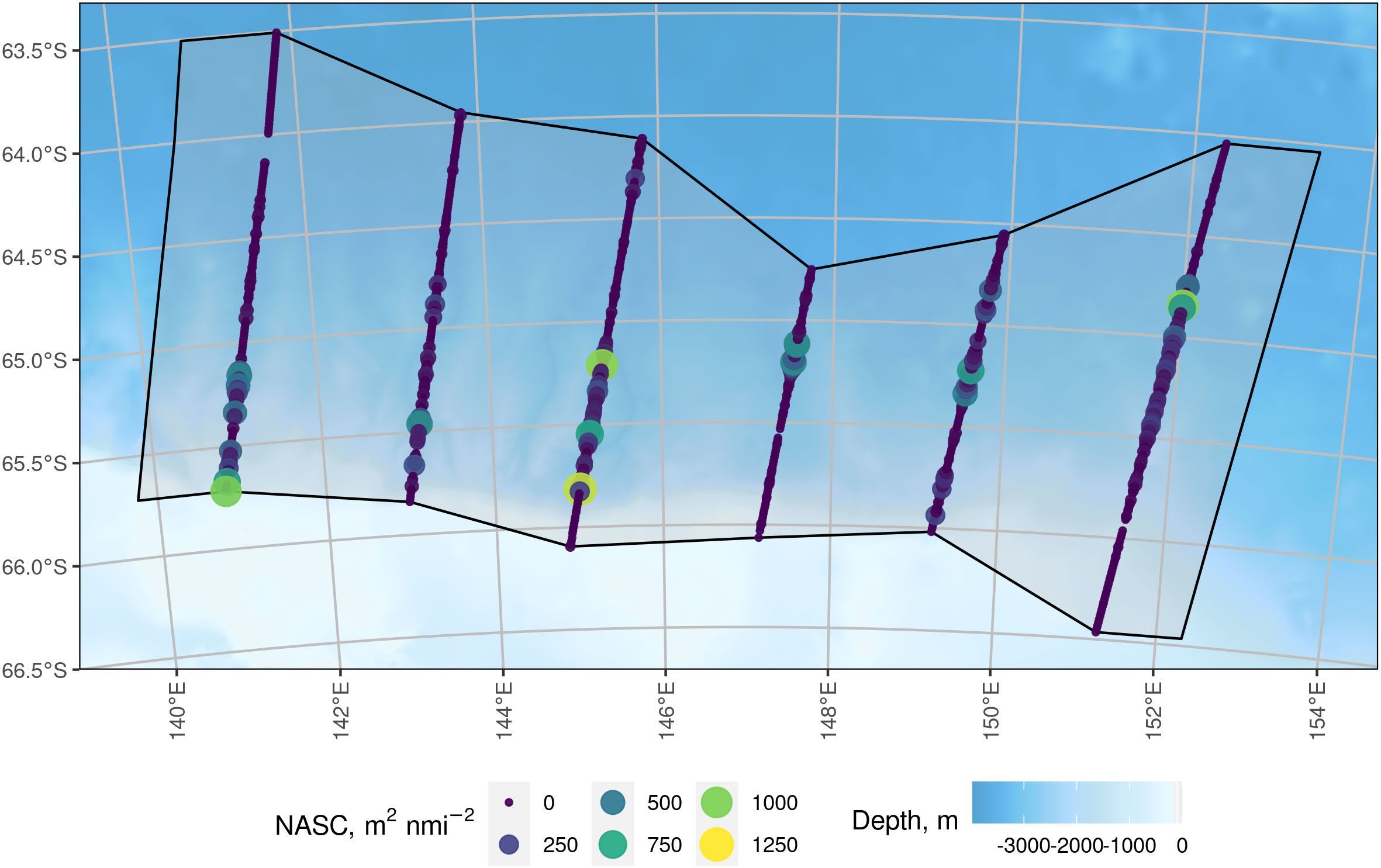
Figure 2 Six parallel transects of acoustic data (coloured circles) within the survey domain (grey shaded with the polygon bounded by a solid black line). The transects ranged in length from 150 km to 270 km. Each circle represents the centre of one nautical mile of 120 kHz acoustic data of krill and the size of the acoustic observation circle is proportional to its Nautical Area Scattering Coefficient value. The survey boundary joins the northern and southern points of each transect and is expanded by half the inter-transect distance (50 km) to the east and west. Background bathymetry is from the General Bathymetric Chart of the Oceans (GEBCO; The GEBCO_2014 Grid, version 20150318, http://www.gebco.net).
The coordinates of both the survey boundary and the acoustic data were projected from geographical coordinates (latitude and longitude) to grid coordinates (Universal Transverse Mercator; UTM). The UTM coordinate system has units of metres which enables sA to be divided into an equally spaced grid. The chosen grid resolution was 1,852 m (1 nautical mile), equal to the echo integration resolution of sA, and was selected to minimise model overfitting whilst maximising the resolution of the spatial model predictions.
Net samples provided measurements of krill length distributions at discrete locations within the survey area and were collected using a rectangular mid-water trawl [RMT 8 + 1; Everson and Bone (1986)] with an 8m2 mouth opening and mesh size of 4.5 mm A total of nL = 4069 lengths (Standard length 1 see Morris et al., 1988) were recorded at 33 locations during the ENRICH voyage and 16 locations during the TEMPO voyage.
Since no krill wetmass data were recorded during the ENRICH voyage, krill length and krill wetmass data from the 2021 TEMPO voyage, were used. The non-linear relationship between krill length, L (measured from the anterior edge of the eye to tip of telson, AT see Morris et al. (1988) their Figure 1, units: mm), and wetmass, (units: g) was estimated using a single model fit W(l) to the 503 recorded values of krill length and wetmass from 16 W(l) locations. Equation 1 was used to model this relationship (Hewitt et al., 2004):
The model parameters, a and b, were estimated by non-linear least squares.
The backscattering cross-sectional area, σbs(l) can be understood as the linear amount of acoustic energy scattered by an individual target. This is a parameter required to scale sA to numerical density. σbs(l) is given by the linear form of the target strength to length relationship at 120 kHz TS =10log10(σbs),calculated using the R package ZooScatR v 0.4, (Gastauer et al., 2019). ZooScatR employs the distorted wave born approximation (DWBA) to calculate TS of weakly scattering organisms, such as krill, (Chu and Ye, 1999). The TS was computed at 120 kHz for lengths between 10 and 70 mm in intervals of 1 mm.
ZooScatR also allows for orientation, material properties, and shape parameterisation of the DWBA through the use of a shape profile that is scalable in length and radius.
A population of krill with varying shape has been shown to produce a more strongly varied TS response than an equivalent shape constant population (Bairstow et al., 2021). We have used the catalogue of shapes described in Bairstow et al. (2021) to assess the influence of shape on biomass estimates.
The mean Procrustes configuration, known as a consensus configuration, of the shape catalogue was again used in this work as a generic, scalable shape (Adams et al., 2004). The results from this generic shape provided a comparison to the results obtained using the shape catalogue to explore the influence of shape on biomass.
The orientation of krill, Figure 1, is known to have a sizeable effect on TS (Calise and Skaret, 2011). Therefore, we have considered the range of reported orientation distributions outlined in Table 1, when calculating the TS to length relationship to assess the influence of orientation on biomass estimates. Of these distributions, only those reported by Lawson et al. (2006) and Kubilius et al. (2015) were measured in situ.
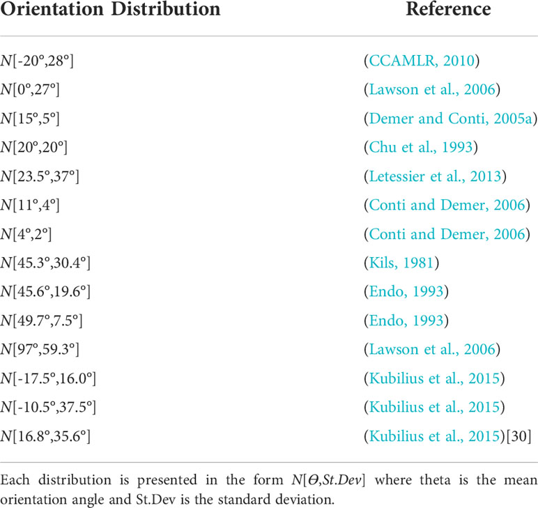
Table 1 Gaussian distributions of krill orientation angle reported in the literature.
The sampling uncertainty arising from the acoustic survey was evaluated by Geostatistical Conditional Simulations [GCS; (Renard et al., 2014)] using the R package RGeostats v12.0.1.
Here, the GCS used a classical Gaussian simulation and this requires the simulated variable, in this case sA to be derived from a Gaussian field. The krill backscatter density data (sA) was heavily zero-inflated. Due to the patchy spatial distribution of many pelagic animals, this is a commonly observed challenge in acoustic data. Before fitting the variogram, the zero-inflated sA data were transformed into a Gaussian distribution using an empirical anamorphosis model [for a detailed explanation see Rivoirard et al. (2008)]. Gaussian values can be estimated directly by GCS for the case of values > 0. A Gibbs sampler was used to iteratively simulate a Gaussian value at each point where sA was equal to 0, conditional on it being lower than a given cut off value and based on the modelled variogram of the data (Woillez et al., 2009; Gastauer et al., 2017).
A total of nsim= 999 GCS of acoustic density simulations across the survey region were performed, i.e. nsim maps of sA were calculated using GCS. Based on nsim, summary statistics (mean, standard deviation and CV) were calculated globally, i.e. across all simulations, and presented here as the CV of sA or locally by simulation results within a given spatial cell. Local simulation results for all spatial cells within the survey area were presented as maps of the mean and standard deviation of sA.
It is important to note that the estimated error from GCS is the sampling error of sA, and should not be confused with the measurement’s stochastic error that can be obtained through Monte Carlo simulations. We used Monte Carlo simulations to calculate the stochastic error of the length and wetmass distributions (see Section 2.7). The same number of simulations were used for the Monte Carlo measurement error as for the GCS which enabled us to combine, on a simulation-by-simulation basis, the GCS simulations of sA with the Monte Carlo simulations to calculate the CV of krill biomass.
The areal biomass density of krill, ρ (units: g m-2), within Asurvey, was calculated by scaling sA (units: m2nmi-2) by a conversion factor, C (units: g nmi2 m-4), Eq. 2.
The conversion factor, C, Eq. 3, is a function of the length distribution (where fi is the relative frequency of occurrence, i.e. the number of krill in the ith length class li), the linear TS to length relationship (σsp(li)) and length to wetmass relationship, W(li). Therefore, C incorporates all variability and uncertainty in biomass of density not associated with sA and Asurvey.
where, σsp is the spherical scattering cross-section [σsp = 4π ×10TS/10, see MacLennan et al. (2002)].
Equation 4 describes how mean density of krill, ρ, was scaled to biomass (units: Mtonnes) using Asurvey.
Net sample data was deemed to be spatially independent. nsim simulations of krill length distributions were produced from the net data by drawing random samples from thew observed lengths with replacement, with net haul as the sampling unit (i.e. a non-parametric bootstrap). To investigate variability in the krill length to wetmass relationship, this sampling procedure was repeated for the nets (n=16) that had krill length and wetmass samples and Eq. 1 refit for each simulated sample.
TS simulations were performed for the in situ measured orientation distributions presented in Table 1 using both the generic shape and the shape catalogue. In the case of the shape catalogue, for each of the nsim simulations, random samples of 61 shapes (one shape per length) were chosen with replacement. Each of the nsim shape simulations were used to compute a TS to length relationship where the shape list gives the shape to be scaled to each length in the relationship. All shapes in the catalogue were assumed to be scalable to any reasonable length. The ratio of length to radius used in the TS calculations was determined by natural ratio of length to radius of the shape in use. In the cases of the generic shape, the ratio of length to radius is given by the average of the shape catalogue.
Simulations of length, wetmass and TS were combined to produce simulations of the conversion factor, C. Areal biomass density, ρ was simulated by combining nsim simulations of C with nsim simulations of the spatially dependent acoustic density,sA. A mean krill density for the survey domain, , was computed by averaging ρ over nsim simulations, Eq. 5.
Simulations of biomass were computed by scaling each of the nsim simulations of areal biomass density . The total biomass was then calculated as the average of biomass estimates over nsim simulations using:
Therefore, the result was nsim values of krill biomass for each combination of shape method (generic or shape catalogue) and orientation distribution.
The acoustic data were collected along six parallel transects with sA values ranging 0 to 1256 m2nmi-2 (Figure 2).
The length frequency distributions for each net haul location had Gaussian distributions with similar means, Figure 3. Therefore, no underlying, spatially dependent structure of the catch data was revealed. In our simulations, the spatial dependence of the catch data was assumed to be negligible and simulations of the length distribution were sampled from the overall measured krill length distribution.
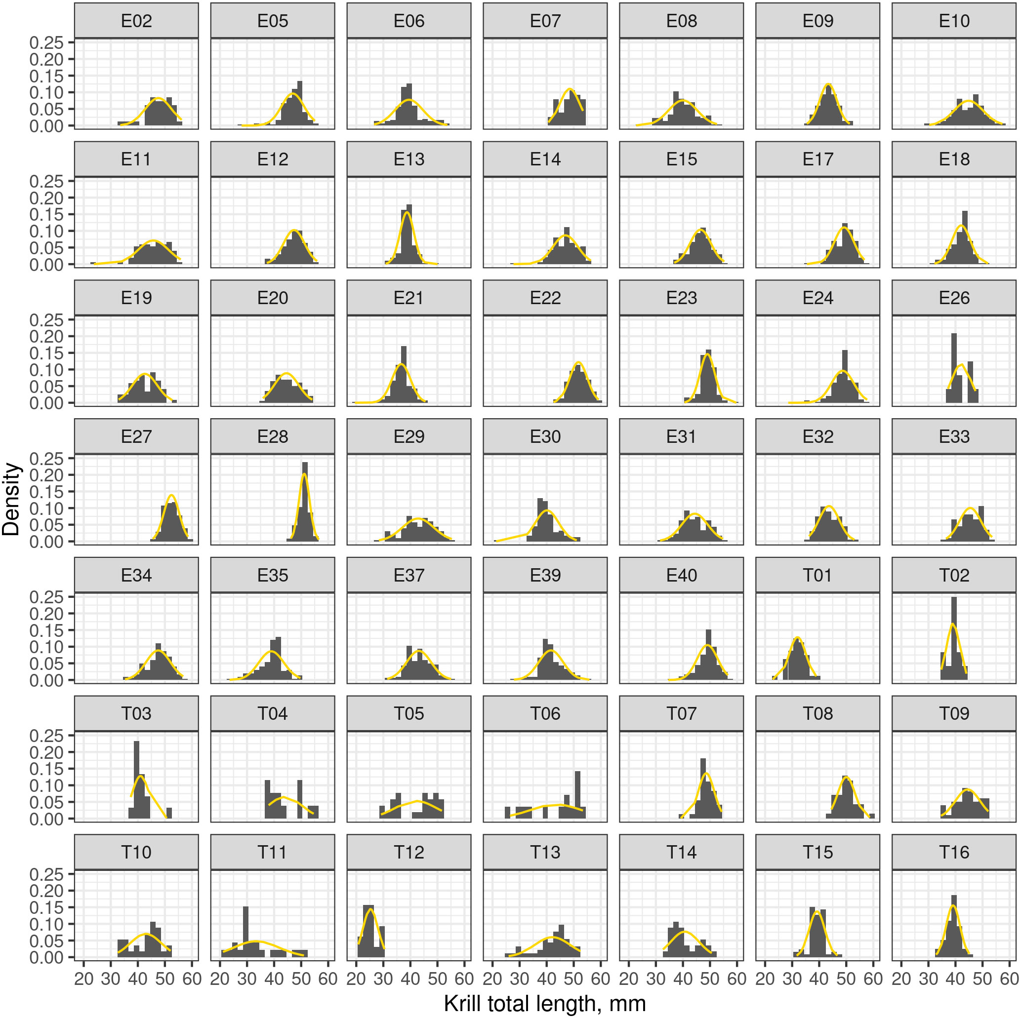
Figure 3 Frequency density plots of krill length recorded from multiple nets. Plots labelled with the prefix “E” indicate catch data from the ENRICH survey and the prefix “T” indicates data from the TEMPO voyage. The dashed orange line is a Gaussian distribution fitted to the length distribution of each for each net.
Figure 4, illustrates the morphological and orientation dependence of krill TS at 120 kHz. In Figure 4 the heatmap represents the TS response of the shape catalogue, which can be compared to the generic shape, the solid orange line. We observe only minimal cross-over between the shape catalogue and the generic shape across a variety of orientation distribution.
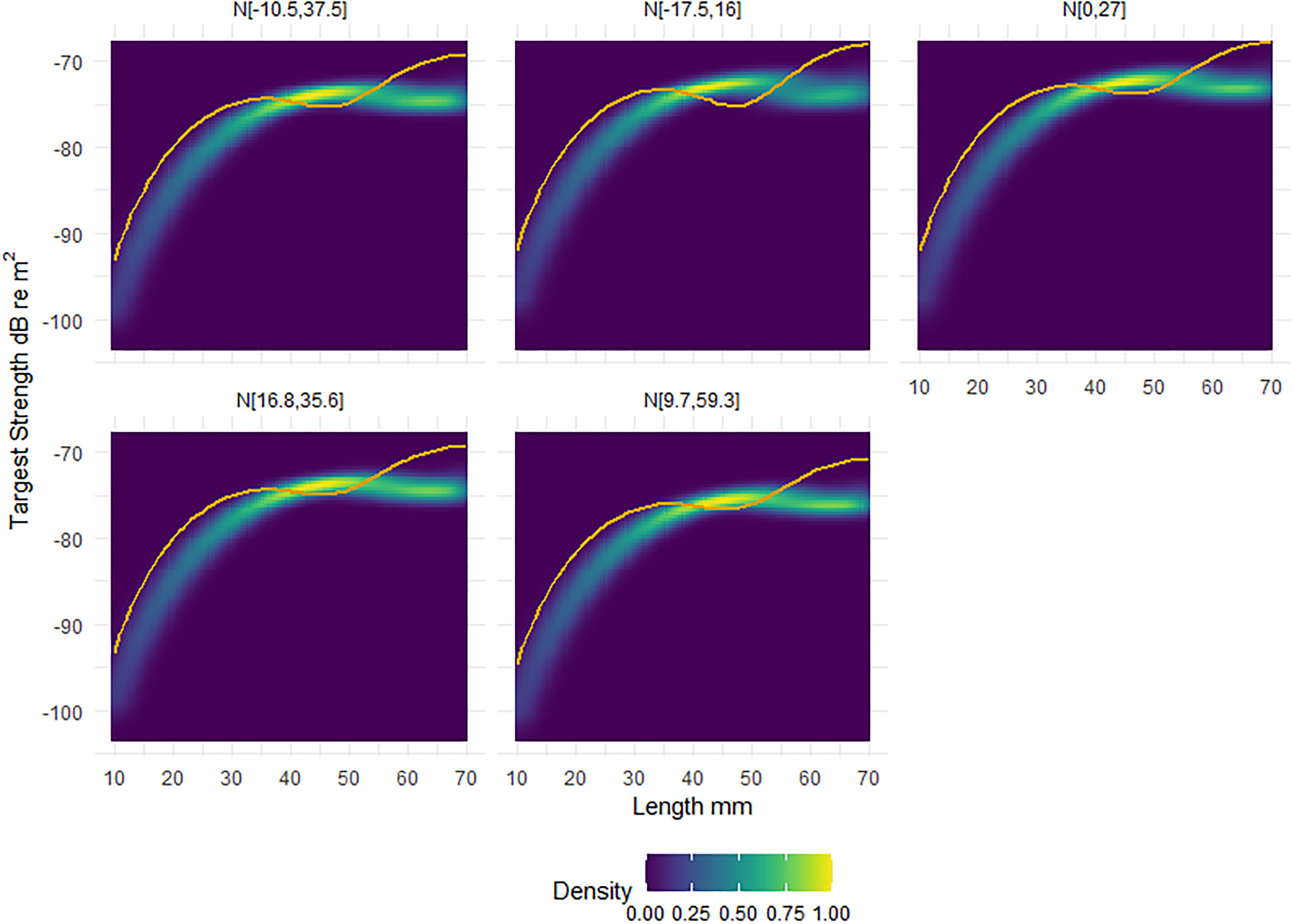
Figure 4 Heatmaps of the standardised relative density, scaled to one, of target strength (TS) responses of the shape catalogue as a function of length. Five orientation distributions, from in situ measurements, were considered: N[-10.5°,37.5rc], N[-17.5°,16°], N[0°,27°], N[16.8°,35.6°], N[9.7°,59.3°]. Overlaid on each panel is the corresponding TS response of the generic shape (orange line). The x axis of length ranges from 10 to 70 mm, with TS calculated each 1 mm interval.
TS was highly dependent on the orientation distribution, Figure 5. For example, the generic krill shape with a length of 30 mm produced TS responses ranging from -106 to -65 dB re m2 over 360° of rotation. Figure 5 displays an example of the interaction between orientation distribution and the relationship between TS and orientation angle. The average TS response over an orientation distribution was highly dependent on where the orientation distribution falls along the TS and orientation angle relationship.
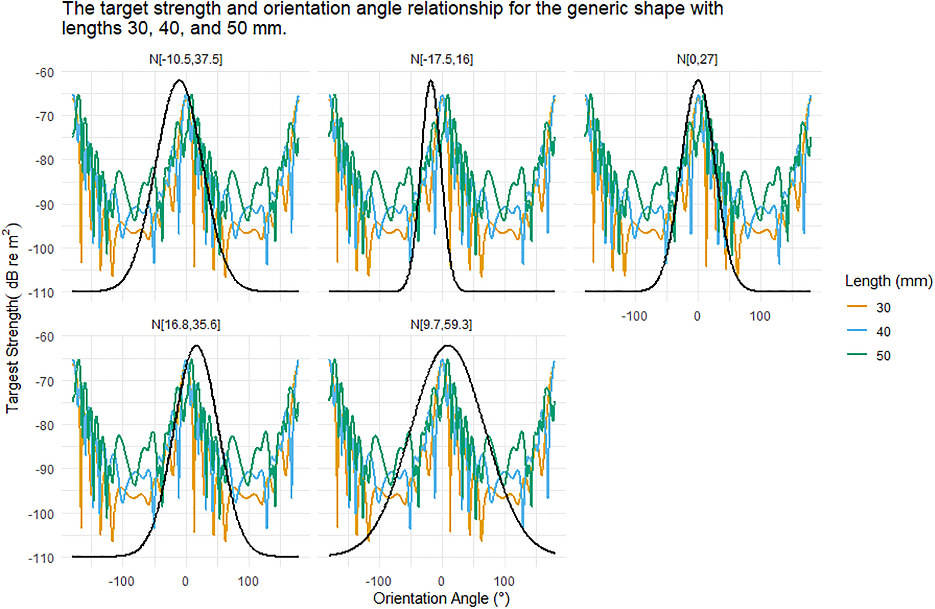
Figure 5 The relationship between target strength (TS) and orientation angle for the generic shape for krill of length 30, 40, and 50 mm is shown in each panel for reference. Each panel displays a different Gaussian orientation distribution N[theta,St.Dev] where theta is the mean orientation angle and St.Dev is the standard deviation. These orientation distributions are centred on or close to 0 degrees. The standard deviations range from 16 to 59.3 degrees. As the standard deviations increase the range of TS responses encompassed also increases, especially as nulls are included.
The orientation distribution N[-17.5°,16°] had the smallest standard deviation of the in situ orientation distributions. This distribution also had the largest magnitude mean orientation angle, despite which the distribution did not encompass the deepest TS nulls, Figure 5. In contrast, the orientation distribution N[-9.7°,59.3°], had the largest standard deviation and encompassed the full range of simulated TS responses, including deep nulls, leading to a lower overall TS response, Figure 5.
Figure 6 displays boxplots of the conversion factor simulations for the shape catalogue and the generic shape for the orientation distributions used in Figure 5. A heatmap of the length to wetmass relationship simulation results, used to calculate the conversion factor, is displayed in Figure 7.
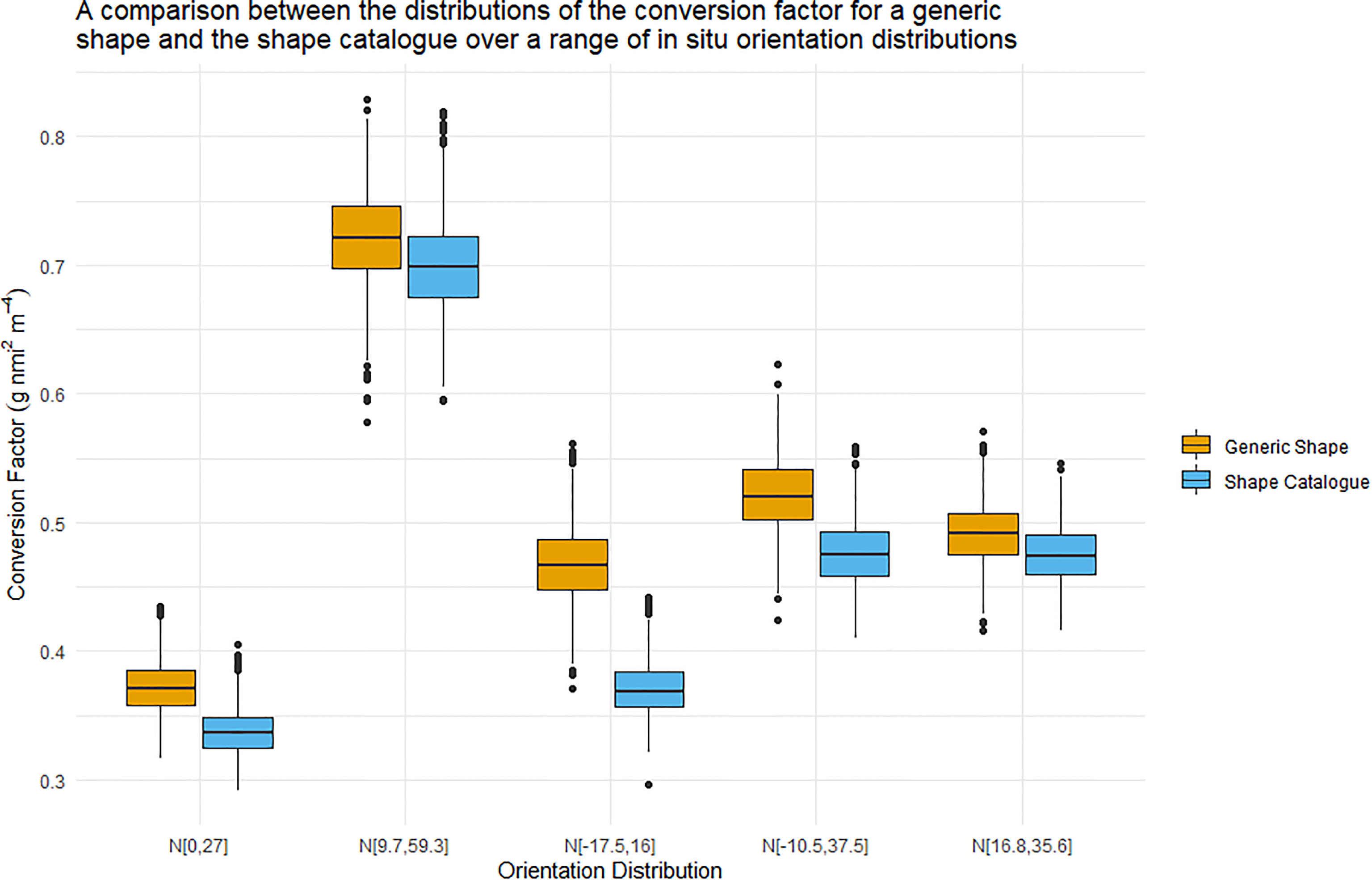
Figure 6 Boxplots illustrating the distribution of the conversion factor for both the generic shape (orange) and the shape catalogue (blue). The five orientation distributions considered here were measured in situ. The central line of each boxplots indicated the median conversion factor value. The boxplot whiskers illustrate the 95th percentile and values outwith this range are indicated by data points.
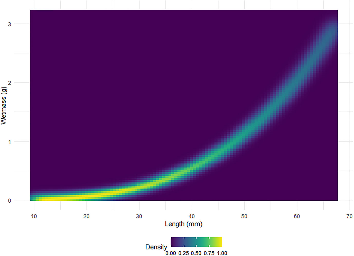
Figure 7 A heatmap of the standardised relative density, scaled to one, of krill wetmass as a function of length. A total of 999 simulations of wetmass are shown.
The interquartile range of the conversion factors produced by the shape catalogue was on average 3.6 times that of the generic shape (standard deviation: 0.3). The median conversion factor value of the generic shape was on average 10% higher than of the shape catalogue, with a maximum difference of 26%.
Due to the highly skewed nature of acoustic data (48% of sA values were zero), prior to kriging, a transformation was required to transform the data into a Gaussian distribution, Figure 8. A variogram was fitted with an iterative least squares method to the transformed acoustic data with a nugget effect (sill: 0.326) and an exponential model (range: 73.6 km, theoretical range: 303 km, sill: 0.701; Figure 9).
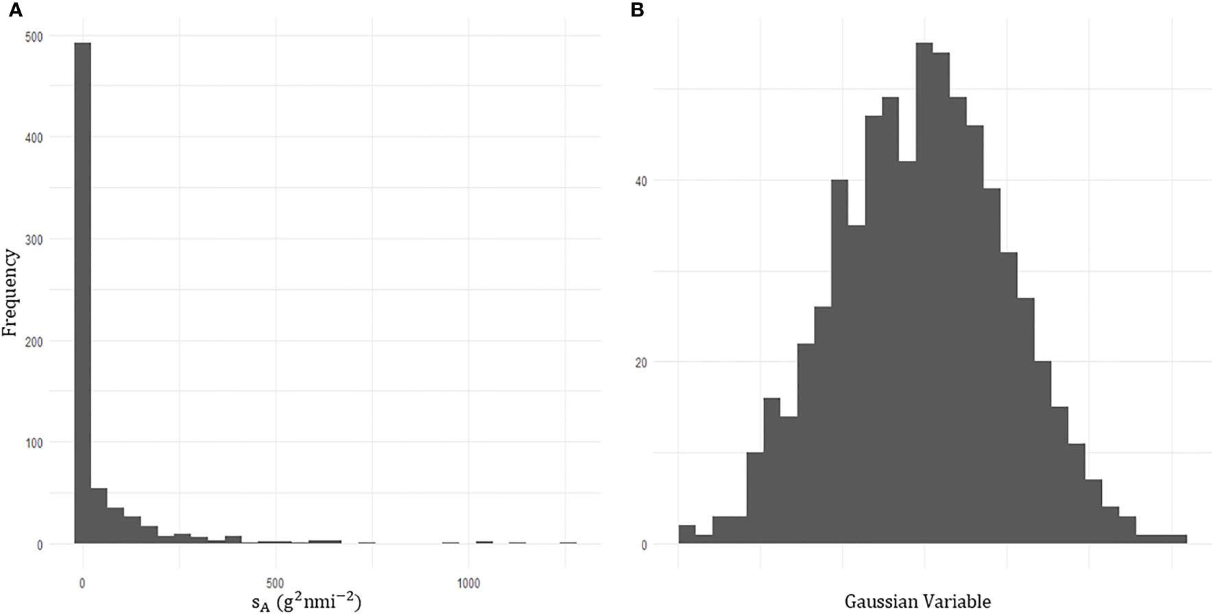
Figure 8 Histograms of the acoustic density attributed to krill echos,sA. (A) The zero inflated acoustic density prior to transformation. (B) Transformed acoustic density data which follows a gaussian distribution.
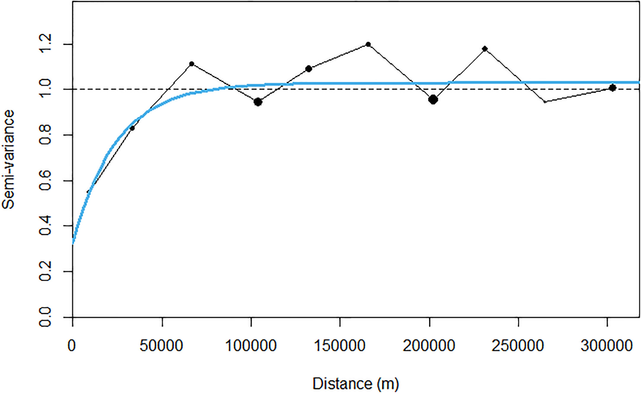
Figure 9 Experimental back transformed (black dots) and modelled (solid blue line) variogram of sA for krill.
The results of the sA simulations are presented in Figure 10. The spatial distribution of sA within the survey area are displayed alongside the corresponding spatial distribution of the standard deviation. The regions of high standard deviation typically correspond to regions of high sA in Figure 10. The sampling variability, i.e. the CV of sA throughout the survey region, calculated by GCS was 16.8%.
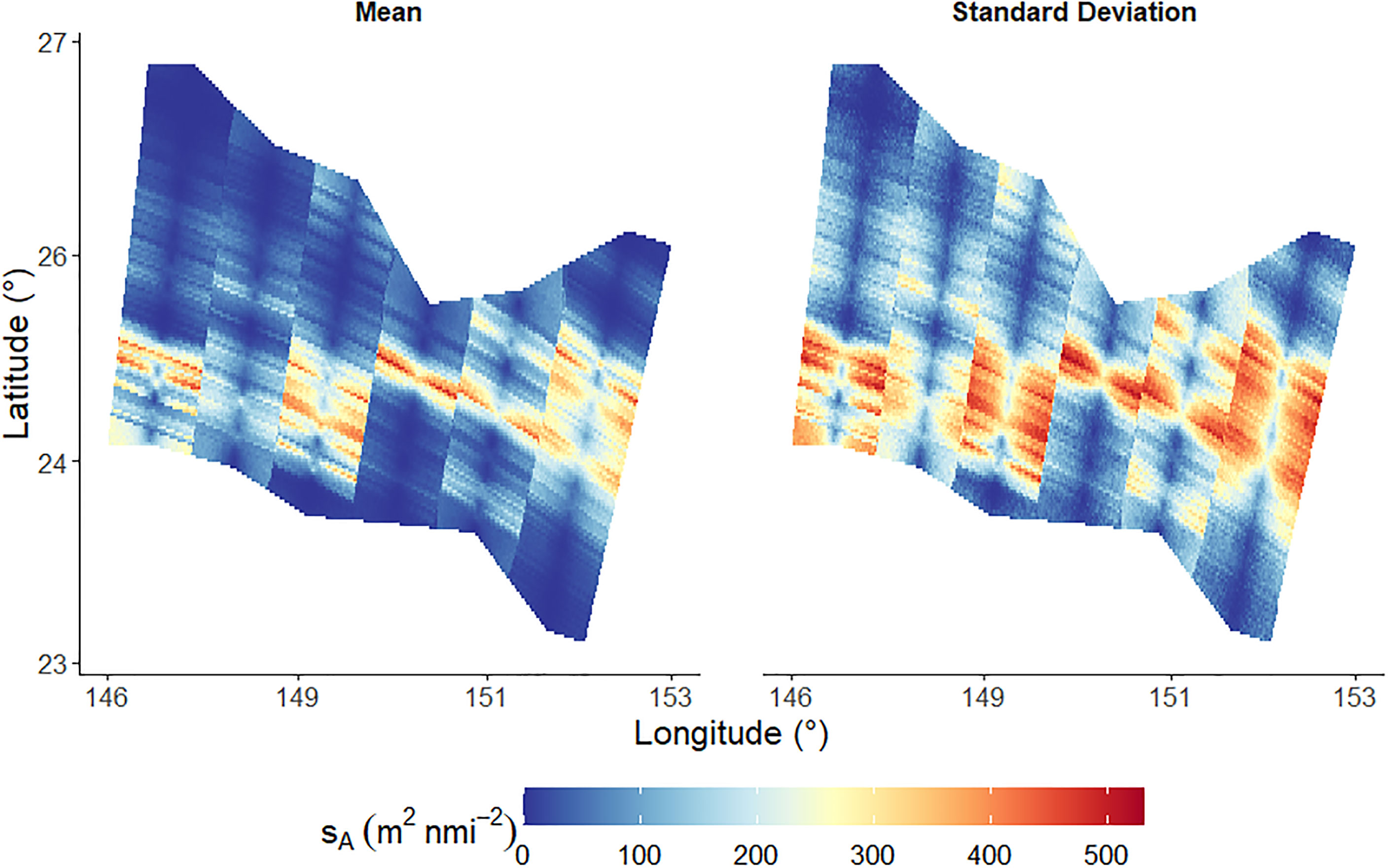
Figure 10 Mean of nsim simulations of Nautical area scattering coefficient, sA. The left plot indicates the mean sA at all locations within the survey domain and the right plot indicates the corresponding mean standard deviations.
The parallel lines observed in Figure 10 divide the survey area into six regions where the centre of each region is an acoustic data transect. These parallel lines are a result of the simulation resolution and the areas of influence of each data point.
Estimates of density and biomass were calculated for the in situ measured orientation distributions using the generic shape and the shape catalogue. Figure 11 illustrates the distributions of the density and biomass estimates. Figure 11 corresponds well to Figure 6 where the orientation distribution N[0°,27°] produced the lowest conversion factors and the lowest density and biomass estimates. Figure 11 is not simply a scaled version of Figure 6 because the variability acoustic data sA is much higher than the variability of the conversion factor, Table 2.
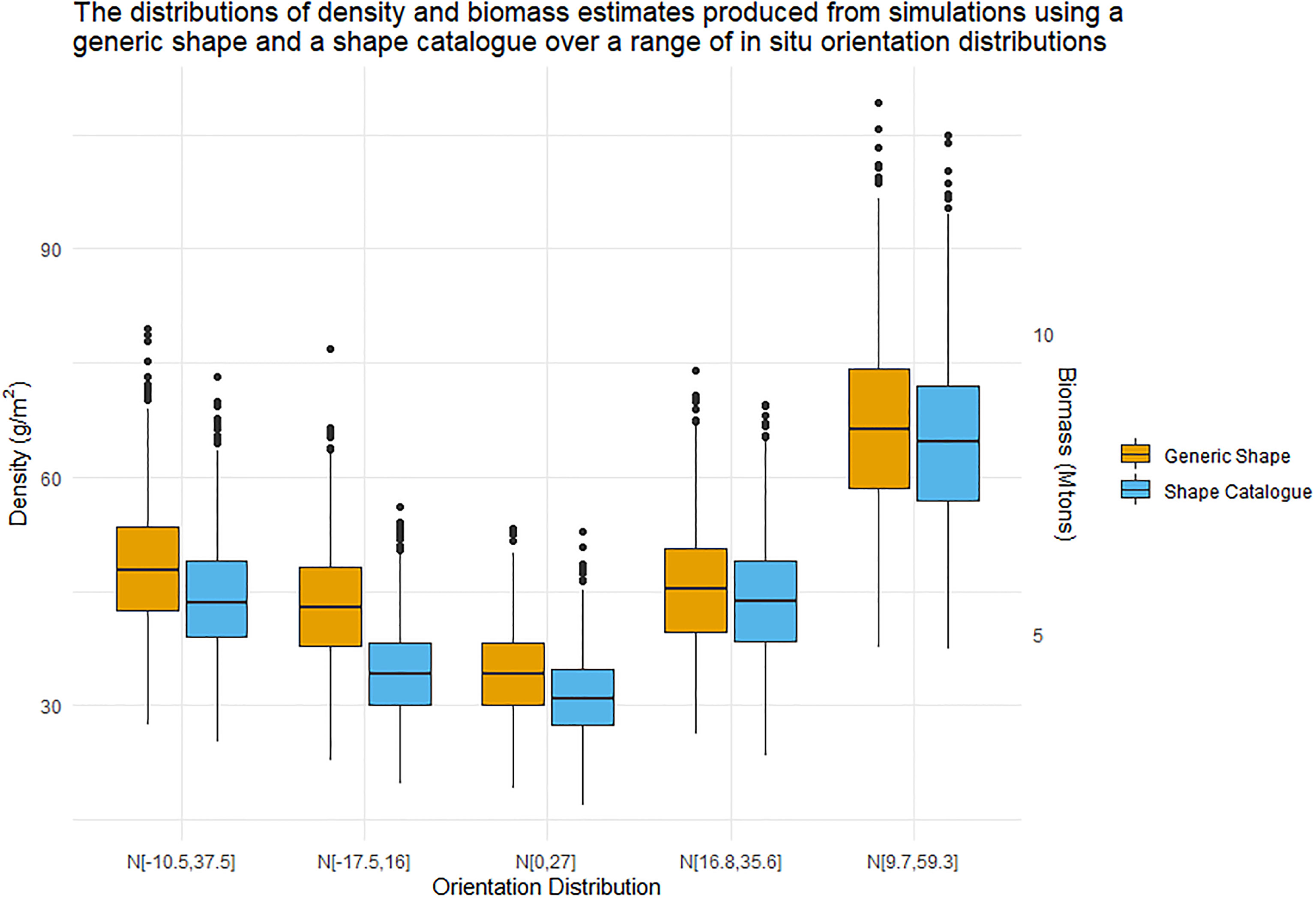
Figure 11 Boxplot distributions of krill density (left Y axis) and biomass (right Y axis) estimates produced by nsim simulations. The central line represents the median density or biomass estimate. These estimates were produced using both the generic shape (orange) and shape catalogue (blue) and five in situ orientation distribution.
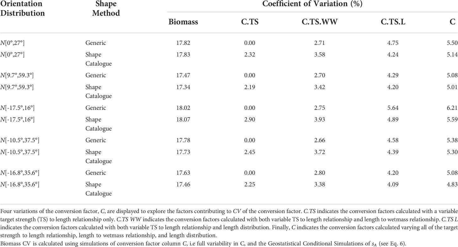
Table 2 Coefficients of variation (CV) for krill biomass and the conversion factor.
Table 2 presents the coefficients of variation (CV) of biomass estimates for each of the five in situ orientation distributions and the generic shape and shape catalogue. The CV of the biomass has two components: the spatial variability of sA due to sampling, and the variability due to the conversion factor. The CV of the conversion factor, which contributes to the CV of biomass, is also included in Table 2. The CV of the conversion factor, can also be further divided into several components: variation due to shape, the krill length to wetmass relationship and the krill length frequency distribution. To explore the contribution of each of these components to the conversion factor variance, the CV conversion factor was presented for three additional cases: (i) where the conversion factor was calculated with a variable TS to length relationship only; (ii) a variable TS to length and length to wetmass relationship, and (ii) a variable TS to length and length distribution. When using the generic shape, only one TS to length relationship is considered, therefore CV of the conversion factor is zero when the length to wetmass relationship and length distribution are constant, CV.TS in Table 2.
The method described in this paper is a quantification of the impact of morphological and behavioural patterns - orientation distribution - on acoustically derived biomass estimates of krill. However, given that hypothetical data (in situ data from three voyages) was used in this work, the presented biomass estimates are not directly actionable in terms of propagation to krill catch limits.
The spatial distribution of krill estimated GCS shows no obvious spatial patterns, such as gradients in krill density, which is expected as the ENRICH survey took place in an oceanic region. Previous acoustic studies of krill in the East Antarctic [e.g. Jarvis et al. (2010) their Figure 4] have shown little spatial structure in krill distribution in oceanic regions.
It is important to recognise that the example data sets used here do not cover the entire range of biologically plausible values of krill that could be observed during a krill survey. For example, juvenile krill are shorter and have a lower mass than adult krill (Morris et al., 1988). Juvenile krill have been observed entering a survey area as a pulse in the krill length frequency distribution [e.g. Hewitt et al. (2003) their Figure 3] leading to a bimodal length distribution. Under such bimodal krill length frequency distributions, we would expect different density and biomass estimates than those given here. This does not represent a failing of the study: our methods are flexible enough to accommodate all biologically plausible krill length frequency distributions. Indeed, a strength of our method is that it will enable exploration of the effect of a variety of krill length frequency (or other krill measurements e.g. orientation distribution Figure 11) on krill density and biomass estimates.
The TS varies considerably with orientation angle (Demer and Conti, 2005; Bairstow et al., 2021). This relationship is a result of the variation in the interference between acoustic waves reflected by the target. At an orientation angle of 0° (broadside incidence) the surface area of the target, perpendicular to the acoustic beam, is at a maximum resulting in a peak in the TS response. At this orientation, the TS response is primarily dependent on the interference between the acoustic waves reflected by the dorsal and ventral interfaces of the krill, Figure 1. Typical acoustic source have frequencies of 38, 70, 120, and 200 kHz resulting in wavelengths in seawater of 39, 21 12 and 8 mm respectively (with a speed of sound in seawater of 1500 ms-1), that are much longer than the krill radius (or effective height due to the orientation, Figure 1). Therefore, the TS response at 0° is mostly the result of constructive interference. As the orientation angle of the target moves away from 0° the TS generally decreases over 90° of rotation. Deep nulls in the TS and orientation angle relationship are typically seen in the intervals -10° to -50° and 13° to 64°. The minimum TS of these nulls depends on the model resolution and the phase of the model. However, experimental measurements are restricted by the instrument noise floor. At these orientations a large proportion of the targets are effectively invisible to the acoustic instrument.
Orientation distributions that encompass deep TS nulls (here as low as -110 dB re 1 m2) result in lower expected TS responses. When propagated to a conversion factor and a density or biomass estimate, these orientation distributions result in higher values than for orientation distributions that avoid these nulls. While an orientation distribution with a large standard deviation is more likely to encompass a TS null, the overall effect of the null is reduced since the weighting of the TS will be more widely distributed.
In Figure 5 the orientation distributions N[9.7°,59.3°] and N[0°,27°] are centred on, or relatively close to 0 ,°however there is a 32.3° difference in standard deviation. While we see that both of these orientation distributions encompass TS nulls, the median biomass produced by these distributions is 8.39 Mtonnes and 4.33 Mtonnes respectively, when using a generic shape. Hence, the range of orientation values or the width of the orientation distribution has a considerable impact on the calculated biomass.
It has been previously reported that TS is highly dependent on shape (Bairstow et al., 2021). A generic shape was unable to sufficiently capture the variability of TS responses produced by a shape-varying population. Figures 4, 6 and 11 illustrate the effect of this same shape catalogue on the TS to length relationship, conversion factors, and density and biomass estimates.
The conversion factor, density and biomass estimates resulting from the generic shape are consistently higher than those produced with the shape catalogue across a number of orientation distributions. This is a result of the natural variation in the ratio of length to radius within the shape catalogue in comparison to the consistent ratio of length to radius used when scaling the generic shape. The original length of the generic shape, 38.35 mm, is small compared length frequency distribution used here. Therefore, by holding the ratio of length to radius constant for the generic shape, TS may be underestimated as the length to radius relationship is non-linear in actual animal populations (Amakasu et al., 2011). The natural variability of ratio of length to radius of the shape catalogue also increases the likelihood of TS nulls at any particular orientation. The constant ratio of length to radius of the generic shape also results in a higher CV for the conversion factor when only the variability of TS and length are considered, Table 2.
The variability of the length, shape, and ratio of length to radius of the shape catalogue results in greater variability of the position of TS nulls compared to the generic shape where only length variability is present. Where an orientation distribution has a narrow standard deviation any nulls are likely to be heavily weighted. Therefore, where the generic shape is used, the conversion factor estimates are artificially inflated, compared to the lower conversion factor estimates when using the shape catalogue due to the more variable null locations. This effect can be seen in Figure 6 for the orientation distribution N[17.5°,16°] where the median conversion factor produced by the generic shape is 26% higher than the median conversion factor produced by the shape catalogue. Conversely, the wider standard deviation of the orientation distribution N[16.8°,35.6°] reduces this effect despite the mean orientation angle falling in a similar region with deep nulls along the TS and orientation angle relationship. For the orientation distribution N[16.8°,35.6°] the median conversion factor produced by the two shape methods differ by only 4%.
Here we have used a single krill length frequency distribution to represent the entire survey area. Over larger survey areas, e.g. BROKE-West (A= 1.5 million km2; Nicol et al. 2010a), that are also well sampled by nets, it is reasonable to examine spatial variation in krill length frequency. Indeed, for BROKE-West Kawaguchi et al. (2010) used cluster analysis and determined there were three length frequency distributions that described the overall survey level krill length frequency distribution. To incorporate length frequency distribution into future krill biomass estimates, we recommend a spatially explicit approach be adopted that takes into account krill length and stage class. We also recommend that the approach includes testing to ensure that the correct number of classes are chosen, including instances where there is one class for a survey. For multivariate approaches, the gap-statistic Tibshirani et al. (2001) can check for single class instances.
We have shown the orientation distribution has the largest effect on biomass estimation. Whilst this effect is well documented, e.g. (Calise and Skaret, 2011), to our knowledge this is the first study to propagate forward the orientation distribution effect to biomass estimation.
The sensitivity of krill TS to orientation, and the widely differing orientation distributions reported in the literature make it difficult to incorporate these into a single biomass estimate. Indeed the widely differing biomass estimates resulting from these orientation distributions, suggests this problem cannot be overcome by using a collection of in situ orientation distribution literature values as we have done here. For future work we suggest the following:
● Rather than a TS model, In situ observation of krill TS using, an acoustic-optical probe or other method, which will provide an observed TS distribution. However we acknowledge the difficulties associated with such methods;
● Alternatively, calculations of the relationship between TS, length and orientation angle could be made using wideband data (Lee et al., 2012);
● Assume a fixed orientation distribution for all surveys (the current approach);
● Where a TS model is being used, a survey specific shape catalogue incorporating shape, length, and ratio of length to radius variability should be implemented.
Meanwhile, when using survey-specific orientation distributions, we recommend being cautious of narrow distributions (distribution standard deviation < 15°) and checking the interaction relationship between TS and orientation angle and the orientation distribution, Figures 4, 5.
The work described in this paper set out to explore the impact of orientation and shape on biomass estimates of Antarctic krill using hypothetical survey data. This method is also applicable to most other acoustic-trawl surveys of aggregating pelagic species.
We found that orientation distribution has the largest impact on biomass estimate. Orientation distributions, especially those with narrow standard deviations, may emphasise the results of deep nulls in the TS to length relationship. This can lead to biologically implausible biomass estimates. We recommend avoiding such situations with careful consideration of orientation distributions or in situ observation of krill TS where possible.
Krill shape and ratio of length to radius also appeared to be important factors in the calculation of biomass estimates. Null locations along the TS and orientation axis are particularly responsive to changes in the ratio of length to radius. Therefore we suggest proper consideration of shape and ratio of length to radius variability should be made using a survey specific shape catalogue.
The orientation distribution N[49.7°,7.5°] was reported by Endo (1993) for hovering krill in an aquarium. The TS length relationship computed with this orientation distribution is displayed in Figure 12 for 120 kHz alongside the responses for a number of other orientation distributions. The orientation distribution N[49.7°,7.5°] typically produces the lowest TS responses across all lengths in addition to a more variable targets strength length relationship.
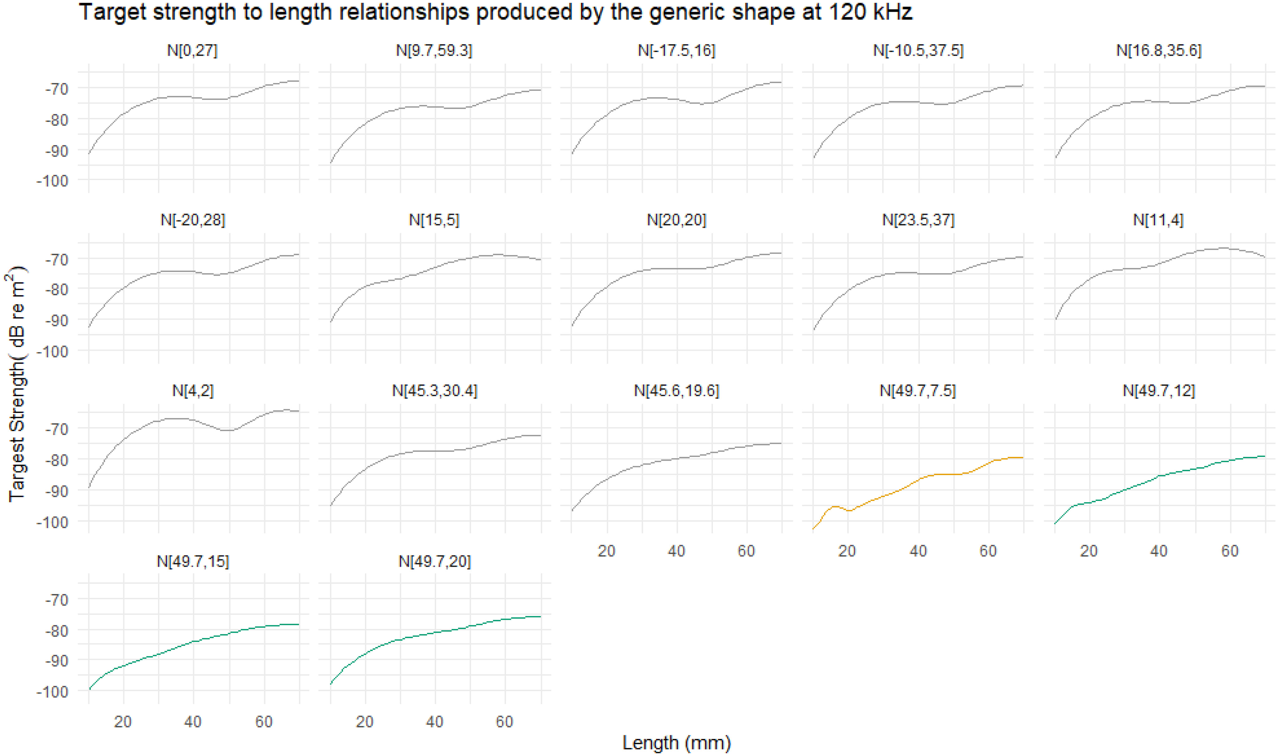
Figure 12 The relationship between target strength (TS) and length at 120 kHz for range of reported orientation distributions. Ten of the eleven reported orientation distributions show a typical relationship, where TS smoothly increases with length. The orientation distribution N[49.7°,7.5°] is highlighted in orange due to the atypical relationship. This distribution generally results in lower TS responses with a more variable relationship between TS and length compared to the other distributions. The results of three further orientation distribution are displayed, in green, to illustrate the effect of increasing the standard deviation of N[49.7°,7.5°]to 12°, 15°, and 20°.
To understand why N[49.7°,7.5°] produces an atypical TS length relationship, we can consider where the orientation distribution falls along the relationship between TS and orientation angle. Figure 13 displays the relationship between TS and orientation angle for krill 30, 40 and 50 mm lengths with each panel overlaid with a particular orientation distribution. The orientation distribution N[49.7°,7.5°] falls in a region with deep TS nulls. These nulls are the result of destructive interference between the reflected acoustic waves. Therefore, at the orientations encompassed by N[49.7°,7.5°] the krill produce only a very small TS response, effectively shielding them from measurements at this wavelength. Increasing the standard deviation of N[49.7°,7.5°] broadens the range of targets strength responses that contribute to the overall TS response.
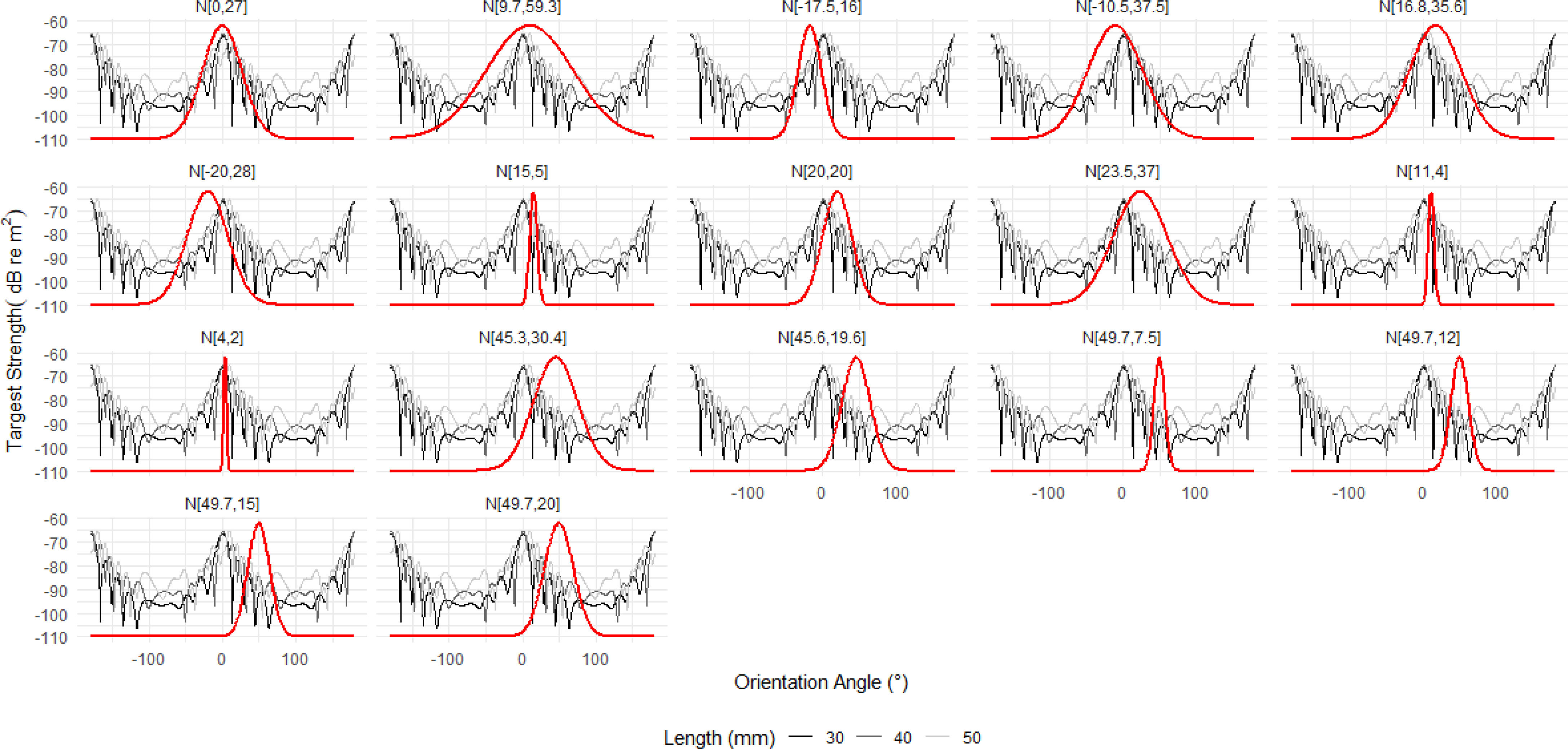
Figure 13 The relationship between target strength (TS) and orientation angle for the average krill shape with lengths 30, 40 and 50 mm is shown for reference. Each panel is overlaid with a Gaussian orientation distribution (solid red line) in the form N[theta,St.Dev], where theta is the mean orientation angle and St.Dev is the standard deviation. The first fourteen orientation distributions are literature values. Of these, N[49.7°,7.5°]falls almost entirely within a region of TS nulls resulting in atypically calculations of the conversion factor. The three addition distributions are the result of increasing the standard deviation of N[49.7°,7.5°] to 12°, 15°, and 20° which broadens the distribution to include more typical TS responses.
Choosing an orientation distribution which falls in a region of a TS null can have a dramatic effect on biomass. Using the TS length relationship at 120 kHz for N[49.7°,7.5°] to calculate the conversion factor and corresponding density and biomass estimates results in unexpectedly high values, Figure 14. However, we also see that increasing the standard deviation of N[49.7°,7.5°] lowers these values towards those of the other orientation distributions as the TS to length relationship reduces in atypicality.
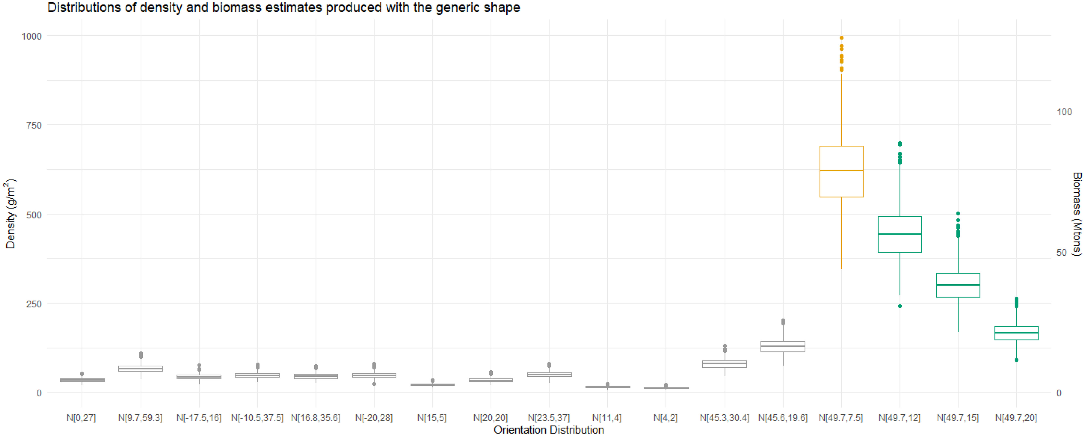
Figure 14 Boxplots of 999 density and biomass estimates for a range of orientation distributions. The midline of the boxplot represents the median estimates. The first fourteen orientation distributions are literature values. Computing the estimates with N[49.7°,7.5°]results in much higher values than for any of the other reported distributions, highlighted in orange. Three additional orientation distributions, highlighted in green, illustrate how increasing the standard deviation of N[49.7°,7.5°] to 12°, 15°, and 20° reduces the estimates.
The suggestion that orientation distributions such as N[49.7°,7.5°] could be realistic for krill poses a problem for biomass estimates using acoustic measurements. If we were confident that the orientation distribution of krill falls within a region of deep TS nulls and has a narrow standard deviation, we could infer the missing data in order to produce realistic biomass measurements. However, there is currently limited consensus as to the most appropriate method to estimate or measure the orientation distribution of a swarm of krill and so we are unlikely to be certain of the orientation distribution. the only alternative is that 120 kHz is deemed unsuitable for acoustic measurements of krill where the measured or estimated orientation distribution has a narrow standard deviation and falls within a region of deep TS nulls. Using an acoustic beam with a longer wavelength may avoid this problem due to the frequency dependence of TS nulls. These results further highlights the need for consistent and accurate measurements of krill orientation to ensure the accuracy of biomass estimates.
The datasets presented in this study can be found in online repositories. The names of the repository/repositories and accession number(s) can be found below: https://doi.org/10.17630/1d26fd16-f574-4fdf-b2f8-a37ec9e6c03d.
FB, SG, SW and MC conducted the modelling studies. TE created Figure 1 and provided technical advice and interpretation of TS spectra. SK assisted with data collection and sample processing and provided technical advice. CB and MC contributed to the conception and design of the study. All authors contributed to the article and approved the submitted version.
FB is funded by an EPSRC studentship (grant code: EP/R513337/1).
We are grateful to the masters, officers, crew, technicians and scientists of R/V Investigator during the ENRICH (IN2017_V01) and TEMPO (IN2019_V01). We thank Robert King, Josh Lawrence, Gavin Macaulay, Dale Maschette, Jessica Melvin and Abigail Smith for measuring krill.
The authors declare that the research was conducted in the absence of any commercial or financial relationships that could be construed as a potential conflict of interest.
All claims expressed in this article are solely those of the authors and do not necessarily represent those of their affiliated organizations, or those of the publisher, the editors and the reviewers. Any product that may be evaluated in this article, or claim that may be made by its manufacturer, is not guaranteed or endorsed by the publisher.
Adams D. C., Rohlf F. J., Slice D. E. (2004). Geometric morphometrics: Ten years of progress following the ‘revolution’. Ital. J. Zool. 71, 5–16. doi: 10.1080/11250000409356545
Amakasu K., Ono A., Moteki M., Ishimaru T. (2011). Sexual dimorphism in body shape of Antarctic krill (Euphausia superba) and its influence on target strength. Polar Sci. 5, 179–186. doi: 10.1016/j.polar.2011.04.005
Bairstow F., Gastauer S., Finley L., Edwards T., Brown C. T. A., Kawaguchi S., et al. (2021). Improving the accuracy of krill target strength using a shape catalog. Front. Mar. Sci. 8. doi: 10.3389/fmars.2021.658384
Calise L., Skaret G. (2011). Sensitivity investigation of the SDWBA Antarctic krill target strength model to fatness, material contrasts and orientation. CCAMLR Sci. 18, 97–122.
CCAMLR (2010). Report of the twenty-ninth meeting of the scientific committee CCAMLR. Hobart, Australia.
Chu D., Foote K. G., Stanton T. K. (1993). Further analysis of target strength measurements of Antarctic krill at 38 and 120 kHz: Comparison with deformed cylinder model and inference of orientation distribution. J. Acoustical Soc. America 93, 2985–2988. doi: 10.1121/1.405818
Chu D., Ye Z. (1999). A phase-compensated distorted wave born approximation representation of the bistatic scattering by weakly scattering objects: Application to zooplankton. J. Acoustical Soc. America 106, 1732–1743. doi: 10.1121/1.428036
Constable A., De la Mare W. (1996). A generalised model for evaluating yield and the long-term status of fish stocks under conditions of uncertainty. CCAMLR Sci. 3, 31–54.
Conti S., Demer D. (2006). Improved parameterization of the SDWBA for estimating krill target strength. ICES J. Mar. Sci. 63, 928–935. doi: 10.1016/j.icesjms.2006.02.007
Demer D. A. (2004). An estimate of error for the CCAMLR 2000 survey estimate of krill biomass. Deep Sea Res. Part II: Topical Stud. Oceanog. 51, 1237–1251. doi: 10.1016/j.dsr2.2004.06.012
Demer D. A., Berger L., Bernasconi M., Bethke E., Boswell K., Chu D., et al. (2015). Calibration of acoustic instruments. Denmark: International Council for the Exploration of the Sea, Copenhagen V
Demer D., Conti S. (2005). New target-strength model indicates more krill in the Southern Ocean. ICES J. Mar. Sci. 62, 25–32. doi: 10.1016/j.icesjms.2004.07.027
Endo Y. (1993). Orientation of Antarctic krill in an aquarium. Nippon Suisan Gakkaishi 59, 465–468. doi: 10.2331/suisan.59.465Endo1993
Everson I. (1977). The living resources of the Southern Ocean Southern Ocean fisheries survey programme (Rome, Italy: FAO).
Everson I., Bone D. (1986). Effectiveness of the RMT8 system for sampling krill (Euphausia superba) swarms. Polar Biol. 6, 83–90. doi: 10.1007/BF00258257
Gastauer S., Chu D., Cox M. J. (2019). ZooScatR–an R package for modelling the scattering properties of weak scattering targets using the distorted wave born approximation. J. Acoustical Soc. America 145, EL102–EL108. doi: 10.1121/1.5085655
Gastauer S., Scoulding B., Parsons M. (2017). Towards acoustic monitoring of a mixed demersal fishery based on commercial data: The case of the northern demersal scalefish fishery (Western Australia). Fisheries Res. 195, 91–104. doi: 10.1016/j.fishres.2017.07.008
Hewitt R. P., Demer D. A. (2000). The use of acoustic sampling to estimate the dispersion and abundance of euphausiids, with an emphasis on Antarctic krill, Euphausia superba. Fisheries Res. 47, 215–229. doi: 10.1016/s0165-7836(00)00171-5
Hewitt R. P., Demer D. A., Emery J. H. (2003). An 8-year cycle in krill biomass density inferred from acoustic surveys conducted in the vicinity of the south Shetland islands during the austral summers of 1991–1992 through 2001–2002. Aquat. Living Resour. 16, 205–213. doi: 10.1016/S0990-7440(03)00019-6
Hewitt R. P., Watkins J., Naganobu M., Sushin V., Brierley A. S., Demer D., et al. (2004). Biomass of Antarctic krill in the Scotia Sea in January/February 2000 and its use in revising an estimate of precautionary yield. Deep Sea Res. Part II: Topical Stud. Oceanog. 51, 1215–1236. doi: 10.1016/j.dsr2.2004.06.011
Howard M. (1989). The convention on the conservation of Antarctic marine living resources: A five-year review. Int. Comp. Law Q. 38, 104–150. doi: 10.1093/iclqaj/38.1.104
Jarvis T., Kelly N., Kawaguchi S., van Wijk E., Nicol S. (2010). Acoustic characterisation of the broad-scale distribution and abundance of Antarctic krill(Euphausia superba) off East Antarctica (30-80°E) in January-March 2006. Deep Sea Res. Part II: Topical Stud. Oceanog. 57, 916–933. doi: 10.1016/j.dsr2.2008.06.013
Kawaguchi S., Nicol S. (2020). “Fisheries and aquaculture,” in Krill fishery (New York: Oxford Univ Pr), 137–158.
Kawaguchi S., Nicol S., Virtue P., Davenport S. R., Casper R., Swadling K. M., et al. (2010). Krill demography and large-scale distribution in the Western indian Ocean sector of the Southern Ocean (CCAMLR division 58.4.2) in austral summer of 2006. Deep Sea Res. Part II: Topical Stud. Oceanog. 57, 934–947. doi: 10.1016/j.dsr2.2008.06.014
Kils U. (1981). Swimming behaviour, swimming performance and energy balance of Antarctic krill Euphausia superba. Biomass Sci 3:1–121.
Kock K. (1985). “Krill consumption by Antarctic notothenioid fish,” in Antarctic Nutrient cycles and food webs Berlin, Heidelberg: Springer, 437–444. doi: 10.1007/978-3-642-82275-9_61
Krafft B. A., Macaulay G. J., Skaret G., Knutsen T., Bergstad O. A., Lowther A., et al. (2021). Standing stock of Antarctic krill (Euphausia superba dana 1850)(euphausiacea) in the Southwest Atlantic sector of the Southern Ocean 2018–19. J. Crustacean Biol. 41, ruab046. doi: 10.1093/jcbiol/ruab046
Kubilius R., Ona E., Calise L. (2015). Measuring in situ krill tilt orientation by stereo photogrammetry: examples for Euphausia superba and Meganyctiphanes norvegica. ICES J. Mar. Science: J. du Conseil 72, 2494–2505. doi: 10.1093/icesjms/fsv077
Lawson G. L., Wiebe P. H., Ashjian C. J., Chu D., Stanton T. K. (2006). Improved parametrization of Antarctic krill target strength models. J. Acoustical Soc. America 119, 232–242. doi: 10.1121/1.2141229
Lee W.-J., Lavery A. C., Stanton T. K. (2012). Orientation dependence of broadband acoustic backscattering from live squid. J. Acoustical Soc. America 131, 4461–4475. doi: 10.1121/1.3701876
Letessier T. B., Kawaguchi S., King R., Meeuwig J. J., Harcourt R., Cox M. J. (2013). A robust and economical underwater stereo video system to observe Antarctic krill (Euphausia superba). Open J. Mar. Sci. 03, 148–153. doi: 10.4236/ojms.2013.33016
MacLennan D. N., Fernandes P. G., Dalen J. (2002). A consistent approach to definitions and symbols in fisheries acoustics. ICES J. Mar. Sci. 59, 365–369. doi: 10.1006/jmsc.2001.1158
Maravelias C. D., Reid D. G., Simmonds E. J., Haralabous J. (1996). Spatial analysis and mapping of acoustic survey data in the presence of high local variability: geostatistical application to north sea herring (Clupea harengus). Can. J. Fisheries Aquat. Sci. 53, 1497–1505. doi: 10.1139/f96-079
Matheron G. (1971). The theory of regionalized variables and their applications (Paris, France: Les cahiers du Centre de Morphologie Mathématique).
Mauchline J., Fisher L. R. (1969). “The biology of euphausiids,” in Advances in marine biology (Academic Press London & New York: Elsevier). doi: 10.1016/s0065-2881(08)60468-x9
Morris D., Watkins J. L., Ricketts C., Buchholz F., Priddle J. (1988). “An assessment of the merits of length and weight measurements of Antarctic krill Euphausia superba,” in British Antarctic Survey bulletin Cambridge UK: British Antarctic Survey, 27–50.
Nicol S., Meiners K., Raymond B. (2010a). BROKE-West, a large ecosystem survey of the South West Indian Socean Sector of the Southern Ocean, 30°E-80°E. Deep Sea Res. Part II: Topical Stud. Oceanog. 57, 693–700. doi: 10.1016/j.dsr2.2009.11.002
Petitgas P. (1993). Geostatistics for fish stock assessments: a review and an acoustic application. ICES J. Mar. Sci. 50, 285–298. doi: 10.1006/jmsc.1993.1031
Petitgas P. (2001). Geostatistics in fisheries survey design and stock assessment: models, variances and applications. Fish Fisheries 2, 231–249. doi: 10.1046/j.1467-2960.2001.00047.x
Reiss C. S., Cossio A. M., Loeb V., Demer D. A. (2008). Variations in the biomass of Antarctic krill (Euphausia superba) around the South Shetland islands 1996–2006. ICES J. Mar. Sci. 65, 497–508. doi: 10.1093/icesjms/fsn033
Rivoirard J., Simmonds J., Foote K. G., Fernandes P., Bez N. (2008). Geostatistics for estimating fish abundance (London, UK: John Wiley & Sons).
Simard Y., Marcotte D., Naraghi K. (2003). Three-dimensional acoustic mapping and simulation of krill distribution in the Saguenay–St. Lawrence marine park whale feeding ground. Aquat. Living Resour. 16, 137–144. doi: 10.1016/S0990-7440(03)00026-3
Tibshirani R., Walther G., Hastie T. (2001). Estimating the number of clusters in a data set via the gap statistic. J. R. Stat. Soc.(Statistical Methodol. 63, 411–423. doi: 10.1111/1467-9868.00293
Trathan P. N., Hill S. L. (2016). “The importance of krill predation in the Southern Ocean,” in Biology and ecology of Antarctic krill (Cham, Switzerland: Springer International Publishing), 321–350. doi: 10.1007/978-3-319-29279-39
Keywords: Antarctic krill, biomass, fisheries acoustics, geostatistics, target strength, wetmass
Citation: Bairstow F, Gastauer S, Wotherspoon S, Brown CTA, Kawaguchi S, Edwards T and Cox MJ (2022) Krill biomass estimation: Sampling and measurement variability. Front. Mar. Sci. 9:903035. doi: 10.3389/fmars.2022.903035
Received: 23 March 2022; Accepted: 28 June 2022;
Published: 22 August 2022.
Edited by:
Jose Luis Iriarte, Austral University of Chile, ChileReviewed by:
Ana Ventero, CNIEO-CSIC, SpainCopyright © 2022 Bairstow, Gastauer, Wotherspoon, Brown, Kawaguchi, Edwards and Cox. This is an open-access article distributed under the terms of the Creative Commons Attribution License (CC BY). The use, distribution or reproduction in other forums is permitted, provided the original author(s) and the copyright owner(s) are credited and that the original publication in this journal is cited, in accordance with accepted academic practice. No use, distribution or reproduction is permitted which does not comply with these terms.
*Correspondence: Martin J. Cox, bWFydGluLmNveEBhYWQuZ292LmF1
Disclaimer: All claims expressed in this article are solely those of the authors and do not necessarily represent those of their affiliated organizations, or those of the publisher, the editors and the reviewers. Any product that may be evaluated in this article or claim that may be made by its manufacturer is not guaranteed or endorsed by the publisher.
Research integrity at Frontiers
Learn more about the work of our research integrity team to safeguard the quality of each article we publish.