Quantifying the Contribution of Each Driving Force to the Lagrangian Residual Velocity in Xiangshan Bay

A three-dimensional numerical model is used to quantitatively evaluate the contribution of each driving force to the Lagrangian residual velocity (LRV) in Xiangshan Bay under conditions of constant buoyancy gradient in time and multi-frequency tide. Each component of the LRV from various processes is derived by tracking each driving force in a tidal period along the particle trajectory. For a comparison of the results, the driving force in the momentum equations is averaged at the fixed points to obtain six components of the Eulerian residual velocity (ERV). A quantitative evaluation of the contribution of each component to the total ERV and total LRV is performed. The sum of the acceleration component, nonlinear advection component, and barotropic pressure gradient component of ERV determines the structure of the total ERV. The LRV is influenced by different dynamic mechanisms. The barotropic pressure gradient component of LRV determines the outflow pattern of the total longitudinal LRV at the surface of the inner Xiangshan Bay, and the density gradient component of LRV is the main determinant of the structure of the total longitudinal LRV at the bottom of the inner Xiangshan Bay. The eddy viscosity component causes the total longitudinal LRV to flow seaward in the Niubi Channel. The sum of the acceleration component and nonlinear advection component of LRV is the main contributor to the inward total longitudinal LRV in the Fodu Channel. The barotropic pressure gradient component leads to total lateral flow in the outer Xiangshan Bay. The collective effect of the components induced by all of the forces determines the structure of the lateral LRV in the inner Xiangshan Bay.

1 Introduction

Coastal plain estuaries are formed at the intersection of an ocean and a river; they typically have abundant natural resources that support human settlement. Accelerated growth of urbanization and industrialization leads to an increase in pollution-related problems in coastal plain estuaries. In this context, it is important to explore exchange circulation and its dynamic mechanisms. Estuarine exchange circulation is described in terms of two types of residual velocity—Eulerian and Lagrangian residual velocities. Eulerian residual velocity (ERV) is the average of the velocities during one or several tidal periods at a fixed location (Abbott, 1960). Lagrangian residual velocity (LRV) is defined as the net displacement of a labeled water parcel over one or several tidal periods (Zimmerman, 1979). When the ERV is used as the inter-tidal transport velocity, the non-conservation “tidal surface source” appears at the surface and the “tidal dispersion” is present in the inter-tidal transport equation (Feng et al., 1984). However, when the LRV acts as the advection velocity, the tidal surface source, and tidal dispersion both vanish in the weakly nonlinear conditions (Feng, 1987), in accordance with the law of mass conservation. Furthermore, Feng et al. (2008) showed that the LRV follows the law of mass conservation in the general nonlinear condition.

In the classical view, Pritchard (1956) proposed that the exchange circulation is mainly induced by the momentum balance of density gradient and friction. Based on the theory of Pritchard (1956); Hansen and Rattray (1965) established the theory of gravitational circulation. The classical analytical theory has been widely used to explore the dynamics of exchange flow. Jeong et al. (2022) indicated the baroclinic effect plays a significant role in residual circulation at the inner harbor in a macro-tidal environment. Zhu et al. (2021) showed friction effect has obvious influences on the structure of residual current. Kobayashi et al. (2022) showed estuarine gravitational circulation has seasonal variability, which is mainly driven by the inhomogeneity of temperature in the lower layer.

However, there are some discrepancies in the simplification of the momentum balance. In addition to the density gradient and friction, many processes have significant influences on exchange flow. Simpson et al. (1990) recognized that the asymmetric stratification induced by the variation of the velocities during flood and ebb has significant influences on estuarine exchange circulation. Jay and Musiak (1994, 1996) emphasized that tidal straining, as described by Simpson et al. (1990), strengthens gravitational circulation. Lerczak and Geyer (2004) indicated that lateral advection significantly influences estuarine exchange circulation. Cheng et al. (2017) showed that when differential advection dominates, lateral advection-induced circulation is landward in the channel and seaward on the shoals; when the Coriolis force dominates, seaward flows and landward flows occupy the right side and left side of the cross section, respectively. Alahmed et al. (2021) investigated the role of the advection and density gradient in the residual circulation in the Gironde estuary in France. Advective accelerations drive inflow in the channel and outflow over the shoals and density gradient has different contributions to the total residual current during neap and spring tides. The effects of eddy viscosity profiles and directional winds on exchange flow are explored by Basdurak et al. (2021). Pein et al. (2018) investigated the transfer of along-channel momentum to lateral circulation by the meander. The meander contributes differently to the lateral circulation during flood tides and ebb tides by influencing the turbulence and centrifugal force. Zhang et al. (2022) found the longitudinal and lateral circulation are modulated by the deepening and narrowing of the estuary. Cui et al. (2018) confirmed that the momentum balance is mainly influenced by not only the pressure gradient and friction but also the advection acceleration and the horizontal diffusion. Chen et al. (2019) indicated that the momentum balance is complex in real geometries. Nonlinear advection plays a significant role in the lateral circulation in the Pearl River Estuary as Coriolis and baroclinic pressure terms, indicating complex dynamic mechanisms of the exchange flow (Xu et al., 2021).

To evaluate the contribution of each component from various processes to total residual velocity, the decomposition methods of estuarine exchange circulation are explored. The empirical orthogonal function (EOF) is extensively used to obtain the components that are induced by various forcing mechanisms (Cerralbo et al., 2018; Valle-Levinson et al., 2019). Sometimes, however, the EOF has no specific physical meaning (Huang et al., 1998). Under weakly nonlinear conditions, a linear decomposition method for the ERV was deduced with zero net river discharge and a rigid lid assumed in a one-dimensional equation (Burchard and Hetland, 2010), and the analytical method was extended for a two-dimensional cross-sectional model (Burchard et al., 2011; Burchard and Schuttelaars, 2012; Burchard et al., 2014). Cheng (2014) removed the limiting, simplified assumptions of Burchard’s methods and extensively developed the decomposition methods by considering the continuity equations; the application of these updated methods in a real bay is a closer reflection of actual conditions. Dijkstra et al. (2017) used a systematic analysis of generation mechanisms and found that exchange flow is influenced by the covariance between shear and eddy viscosity at twice the dominant tidal frequency. The dynamic mechanisms of the interaction among the asymmetric tidal turbulence, the estuarine circulation, and salt transport in short estuaries are explored by Wei et al. (2021). However, those decomposition methods are restricted to the ERV and a weakly nonlinear condition. To understand the mechanisms of the LRV, Jiang and Feng (2014) decomposed tidal body force into three terms with specific physical meanings and determined the quantitative contribution of these terms to the LRV under the condition of constant eddy viscosity. Cui et al. (2019a) used a semi-analytical method to quantify the role of the Stokes’ drift stress term, the nonlinear advection term, and the Coriolis effect of the local acceleration derived from the tidal body force in the LRV. An improved version of the method was used for a wide bay (Cui et al., 2019b). Chen et al. (2020) derived the analytical solution for the LRV with vertically varying eddy viscosity and evaluated the contribution of the Stokes’ drift stress term and the nonlinear advection-induced LRV to the total LRV under weakly nonlinear conditions. However, the two studies did not consider temporal eddy viscosity. Deng et al. (2017) performed a qualitative study of the effects of nonlinear eddy viscosity on the LRV; however, they did not perform a quantitative evaluation of the contribution of each component to the total LRV. Liu et al. (2021) derived the Lagrangian mean momentum equation for measuring the initial time dependence of wind-driven and density-driven LRV. However, a general decomposition of the dynamic mechanisms of the LRV has not yet been developed.

Xiangshan Bay is located in the north of Zhejiang Province, to the south of Hangzhou Bay (Figure 1). It is a narrow and semi-closed bay on the edge of the East Sea. The bay is separated into the inner Xiangshan Bay and the outer Xiangshan Bay. The outer Xiangshan Bay includes the Niubi Channel and the Fodu Channel, which connect to the East China Sea. The bay extends across approximately 70 km, from the mouth to the head. The greatest width of the bay is 20 km, at the mouth, and the narrowest is approximately 3 km, in the middle of the bay. The average depth is approximately 10 m, and the maximum depth is 70 m. The total area of the bay is approximately 560 km², of which more than one third is accounted for by tidal flats. The tidal range increases gradually from the mouth to the head of the bay. The difference between the high tide and the low tide increases as the tidal wave propagates upstream along the bay, indicating strong nonlinearity in the bay. The river discharge of the bay is small, and the wind is weak because the bay is surrounded by mountains and hills. The horizontal stratification in summer is high due to the influence of the Taiwan Warm Current, whereas in winter the difference in salinity between the mouth and the head of the bay is approximately 2 psu, indicating weak horizontal stratification. The main tidal constituent is semi-diurnal M₂, with an amplitude that is two times that of the second major constituent (S₂). Studies on the LRV in Xiangshan Bay have been limited to qualitative analysis in the outer Xiangshan Bay (Xu et al., 2016). Few studies have explored the dynamic mechanisms of the LRV in the bay.

FIGURE 1

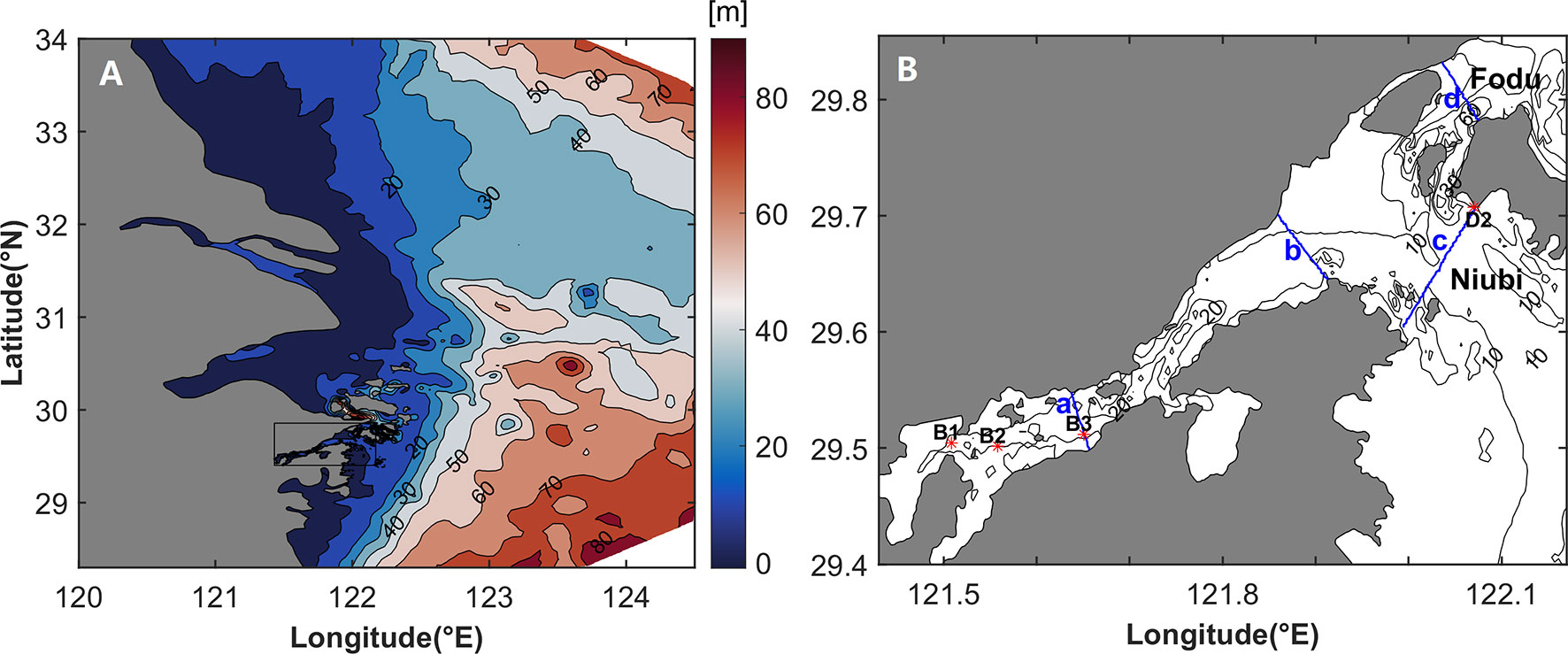
Figure 1 (A) Bathymetry of model domain (shading). The black rectangular box represents the position of the Xiangshan Bay. (B) Bathymetry of Xiangshan Bay (contours), schematic of the positions of four stations (red stars) and four cross sections (blue lines): (a) represents the cross section of the middle of the inner Xiangshan Bay, (b) represents the cross section of the mouth of the inner Xiangshan Bay, (c) represents the cross section of the Niubi Channel, and (d) represents the cross section of the Fodu Channel.

The aim of this study is to determine the contribution of the components induced by each force to the total LRV in Xiangshan Bay. This paper is structured as follows. A description of the parameters for the model setup, validation of the model, and decomposition methods is provided in Section 2. The contribution of each component to the total ERV and the total LRV is discussed in Section 3. The discussion and conclusions are presented in Section 4.

2 Methodology

2.1 Formulation

The momentum equations in sigma coordinates are as follows:

$\begin{array}{ll}\begin{array}{c}\frac{\partial uD}{D\partial t}+\frac{\partial u^{2}D}{D\partial x}+\frac{\partial uvD}{D\partial y}+\frac{\partial u\omega D}{D\partial \sigma }-fv\\ =-g\frac{\partial \zeta }{\partial x}+\frac{1}{D^2}\frac{\partial }{\partial \sigma }\left(v_h\frac{\partial u}{\partial \sigma }\right)-\frac{g}{{\rho }_0}\left(D{\displaystyle {\int }_{\sigma }^0\frac{\partial \rho }{\partial x}d{\sigma }_1-\frac{\partial D}{\partial x}{\displaystyle {\int }_{\sigma }^0{\sigma }_1\frac{\partial \rho }{\partial {\sigma }_1}d{\sigma }_1}}\right)\\ +F_x,\end{array}& (1)\end{array}$

$\begin{array}{ll}\begin{array}{c}\frac{\partial vD}{D\partial t}+\frac{\partial uvD}{D\partial x}+\frac{\partial v^{2}D}{D\partial y}+\frac{\partial v\omega D}{D\partial \sigma }+fu\\ =-g\frac{\partial \zeta }{\partial y}+\frac{1}{D^2}\frac{\partial }{\partial \sigma }\left(v_h\frac{\partial v}{\partial \sigma }\right)-\frac{g}{{\rho }_0}\left(D{\displaystyle {\int }_{\sigma }^0\frac{\partial \rho }{\partial y}d{\sigma }_1-\frac{\partial D}{\partial y}{\displaystyle {\int }_{\sigma }^0{\sigma }_1\frac{\partial \rho }{\partial {\sigma }_1}d{\sigma }_1}}\right)+F_y,\end{array}& (2)\end{array}$

where u (x, y, σ, t), v (x, y, σ, t), and ω (x, y, σ, t) are the velocity components in the longitudinal (x), lateral (y), and dimensionless vertical (σ) directions, respectively. Here, D = H + ζ, where H (x, y) is the mean depth of water, ζ ( x, y, t) is the water surface elevation, t is the time, ρ (x, y, σ, t) is the water density, ρ₀ is the reference density, f is the Coriolis parameter, and v_h (x, y, σ, t) is the vertical eddy viscosity.

ERV is defined as the average of the current velocities over one or several tidal periods at a specific location (Abbott, 1960):

$\begin{array}{ll}{u}_E=\frac{1}{nT}{\displaystyle {\int }_{t_0}^{t_0+nT}u\left(\overrightarrow{x_0} ,t\right)dt=\left|u\right|,}& (3)\end{array}$

$\begin{array}{ll}{v}_E=\frac{1}{nT}{\displaystyle {\int }_{t_0}^{t_0+nT}v\left(\overrightarrow{x_0} ,t\right)dt=\left|v\right|,}& (4)\end{array}$

where n = 1, $\overrightarrow{x_0}$ represents the parcel position, and the Eulerian-averaged operator is defined as follows, with T representing the tidal period and t₀ denoting the start time:

$\begin{array}{ll}\left|·\right|=\frac{1}{T}{\displaystyle {\int }_{t_0}^{t_0+T}·\left(\overrightarrow{x_0} ,t\right)dt.}& (5)\end{array}$

LRV is defined as the net displacement of a labeled water parcel over one or several tidal periods (Zimmerman, 1979):

$\begin{array}{ll}{u}_L=\frac{1}{nT}{\displaystyle {\int }_{t_0}^{t_0+nT}u\left(\overrightarrow{x}\left(t,\overrightarrow{x_0} ,t_0\right),t\right)}dt=\langle u\rangle ,& (6)\end{array}$

$\begin{array}{ll}{v}_L=\frac{1}{nT}{\displaystyle {\int }_{t_0}^{t_0+nT}v\left(\overrightarrow{x}\left(t,\overrightarrow{x_0,}{t}_0\right),t\right)}dt=\langle v\rangle ,& (7)\end{array}$

where n = 1, $\overrightarrow{x_0}$ is the initial parcel position when t = t₀, and $\overrightarrow{x}$ is the parcel position at time t.

The Lagrangian-averaged operator is defined as follows:

$\begin{array}{ll}\langle ·\rangle =\frac{1}{T}{\displaystyle {\int }_{t_0}^{t_0+T}·\left(\overrightarrow{x}\left(t,\overrightarrow{x_0,}{t}_0\right),t\right)dt.}& (8)\end{array}$

The Eulerian-averaged and Lagrangian-averaged operators can be used to not only calculate the ERV and LRV but also analyze the momentum equations at the intertidal scale.

2.1.1 The Eulerian-Averaged Equations

Equations (1) and (2) are averaged at the fixed points in a tidal period, based on Equation (5):

$\begin{array}{ll}\begin{array}{cc}\left|-fv\right|=\left|-\frac{\partial uD}{D\partial t}\right|+\left|-\frac{\partial u^{2}D}{D\partial x}-\frac{\partial uvD}{D\partial y}-\frac{\partial u\omega D}{D\partial \sigma }\right|+\left|-g\frac{\partial \zeta }{\partial x}\right|& +\left|\frac{1}{D^2}\frac{\partial }{\partial \sigma }\left(v_h\frac{\partial u}{\partial \sigma }\right)\right|+\left|-\frac{g}{{\rho }_0}\left(D{\displaystyle {\int }_{\sigma }^0\frac{\partial \rho }{\partial x}d{\sigma }_1-\frac{\partial D}{\partial x}{\displaystyle {\int }_{\sigma }^0{\sigma }_1\frac{\partial \rho }{\partial {\sigma }_1}d{\sigma }_1}}\right)\right|+\left|F_x\right|, \end{array}& (9)\end{array}$

$\begin{array}{ll}\begin{array}{c}\left|fu\right|=\left|-\frac{\partial vD}{D\partial t}\right|+\left|-\frac{\partial uvD}{D\partial x}-\frac{\partial v^{2}D}{D\partial y}-\frac{\partial v\omega D}{D\partial \sigma }\right|+\left|-g\frac{\partial \zeta }{\partial y}\right|\\ +\left|\frac{1}{D^2}\frac{\partial }{\partial \sigma }\left(v_h\frac{\partial v}{\partial \sigma }\right)\right|+\left|-\frac{g}{{\rho }_0}\left(D{\displaystyle {\int }_{\sigma }^0\frac{\partial \rho }{\partial y}d{\sigma }_1-\frac{\partial D}{\partial y}}{\displaystyle {\int }_{\sigma }^0{\sigma }_1\frac{\partial \rho }{\partial {\sigma }_1}d{\sigma }_1}\right)\right|+\left|F_y\right|.\end{array}& (10)\end{array}$

Equations (9) and (10) are divided by the Coriolis parameter to obtain the components induced by various driving forces, based on Equations (3) and (4):

$\begin{array}{ll}\begin{array}{c}{v}_E=(\left|-\frac{\partial uD}{D\partial t}\right|+\left|-\frac{\partial u^{2}D}{D\partial x}-\frac{\partial uvD}{D\partial y}-\frac{\partial u\omega D}{D\partial \sigma }\right|+\left|-g\frac{\partial \zeta }{\partial x}\right|\\ +\left|-\frac{g}{{\rho }_0}\left(D{\displaystyle {\int }_{\sigma }^0\frac{\partial \rho }{\partial x}d{\sigma }_1-\frac{\partial D}{\partial x}{\displaystyle {\int }_{\sigma }^0{\sigma }_1\frac{\partial \rho }{\partial {\sigma }_1}d{\sigma }_1}}\right)\right|+\left|\frac{1}{D^2}\frac{\partial }{\partial \sigma }\left(v_h\frac{\partial u}{\partial \sigma }\right)\right|+\left|F_x\right|)/\left(-f\right), \end{array}& (11)\end{array}$

$\begin{array}{ll}\begin{array}{c}{u}_E=(\left|-\frac{\partial vD}{D\partial t}\right|+\left|-\frac{\partial uvD}{D\partial x}-\frac{\partial v^{2}D}{D\partial y}-\frac{\partial v\omega D}{D\partial \sigma }\right|+\left|-g\frac{\partial \zeta }{\partial y}\right|\\ +\left|-\frac{g}{{\rho }_0}\left(D{\displaystyle {\int }_{\sigma }^0\frac{\partial \rho }{\partial y}d{\sigma }_1-\frac{\partial D}{\partial y}{\displaystyle {\int }_{\sigma }^0{\sigma }_1\frac{\partial \rho }{\partial {\sigma }_1}d{\sigma }_1}}\right)\right|+\left|\frac{1}{D^2}\frac{\partial }{\partial \sigma }\left(v_h\frac{\partial v}{\partial \sigma }\right)\right|+\left|F_y\right|)/f,\end{array}& (12)\end{array}$

$\begin{array}{ll}{u}_E=u_{Eac}+u_{Ead}+u_{Eba}+u_{Egr}+u_{Etu}+u_{Eho},& (13)\end{array}$

$\begin{array}{ll}{v}_E=v_{Eac}+v_{Ead}+v_{Eba}+v_{Egr}+v_{Etu}+v_{Eho}.& (14)\end{array}$

The term $\left|-\frac{\partial uD}{D\partial t}\right|/\left(-f\right)$ and $\left|-\frac{\partial vD}{D\partial t}\right|/f$ represent the acceleration components of ERV (v_Eac and u_Eac); $\left|-\frac{\partial u^{2}D}{D\partial x}-\frac{\partial uvD}{D\partial y}-\frac{\partial u\omega D}{D\partial \sigma }\right|/\left(-f\right)$ and $\left|-\frac{\partial uvD}{D\partial x}-\frac{\partial v^{2}D}{D\partial y}-\frac{\partial v\omega D}{D\partial \sigma }\right|/f$ represent the nonlinear advection components of ERV (v_Ead and u_Ead); $\left|-g\frac{\partial \zeta }{\partial x}\right|/\left(-f\right)$ and $\left|-g\frac{\partial \zeta }{\partial y}\right|/f$ represent the barotropic pressure gradient components of ERV (v_Eba and u_Eba); $\left|-\frac{g}{{\rho }_0}\left(D{\displaystyle {\int }_{\sigma }^0\frac{\partial \rho }{\partial x}d{\sigma }_1-\frac{\partial D}{\partial x}{\displaystyle {\int }_{\sigma }^0{\sigma }_1\frac{\partial \rho }{\partial {\sigma }_1}d{\sigma }_1}}\right)\right|/\left(-f\right)$ and $\left|-\frac{g}{{\rho }_0}\left(D{\displaystyle {\int }_{\sigma }^0\frac{\partial \rho }{\partial y}d{\sigma }_1-\frac{\partial D}{\partial y}{\displaystyle {\int }_{\sigma }^0{\sigma }_1\frac{\partial \rho }{\partial {\sigma }_1}d{\sigma }_1}}\right)\right|/\left(f\right)$ represent the density gradient components of ERV (v_Egr and u_Egr); $\left|\frac{1}{D^2}\frac{\partial }{\partial \sigma }\left(v_h\frac{\partial u}{\partial \sigma }\right)\right|/\left(-f\right)$ and $\left|\frac{1}{D^2}\frac{\partial }{\partial \sigma }\left(v_h\frac{\partial v}{\partial \sigma }\right)\right|/\left(f\right)$ represent the eddy viscosity components of ERV (v_Etu and u_Etu); and |F_x|/(−f) and |F_y|/(f) represent the horizontal diffusion components of ERV (v_Eho and u_Eho).

2.1.2 The Lagrangian-Averaged Equations

Each term in Equations (1) and (2) is integrated along the particle trajectories in a tidal period and divided by the time period to obtain each Lagrangian-averaged force. The variables u, v, ω, ζ, v_h, ρ in each force are the functions of the initial position, initial phase, real-time position, and real time in the tracking process. The tracking algorithm uses a constant time step of 30 s. During each time step, each forcing term is interpolated linearly according to the real-time position and real time, and is integrated using the fourth-order Runge–Kutta time-stepping scheme.

$\begin{array}{ll}\begin{array}{cc}\langle -fv\rangle =\langle -\frac{\partial uD}{D\partial t}-\frac{\partial u^{2}D}{D\partial x}-\frac{\partial uvD}{D\partial y}-\frac{\partial u\omega D}{D\partial \sigma }\rangle +\langle -g\frac{\partial \zeta }{\partial x}\rangle & +\langle \frac{1}{D^2}\frac{\partial }{\partial \sigma }\left(v_h\frac{\partial u}{\partial \sigma }\right)\rangle +\langle -\frac{g}{{\rho }_0}\left(D{\displaystyle {\int }_{\sigma }^0\frac{\partial \rho }{\partial x}d{\sigma }_1-\frac{\partial D}{\partial x}}{\displaystyle {\int }_{\sigma }^0{\sigma }_1\frac{\partial \rho }{\partial {\sigma }_1}d{\sigma }_1}\right)\rangle +\langle F_x\rangle ,\end{array}& (15)\end{array}$

$\begin{array}{ll}\begin{array}{c}\langle fu\rangle =\langle -\frac{\partial vD}{D\partial t}-\frac{\partial uvD}{D\partial x}-\frac{\partial v^{2}D}{D\partial y}-\frac{\partial v\omega D}{D\partial \sigma }\rangle +\langle -g\frac{\partial \zeta }{\partial y}\rangle \\ +\langle \frac{1}{D^2}\frac{\partial }{\partial \sigma }\left(v_h\frac{\partial v}{\partial \sigma }\right)\rangle +\langle -\frac{g}{{\rho }_0}\left(D{\displaystyle {\int }_{\sigma }^0\frac{\partial \rho }{\partial y}d{\sigma }_1-\frac{\partial D}{\partial y}{\displaystyle {\int }_{\sigma }^0{\sigma }_1\frac{\partial \rho }{\partial {\sigma }_1}d{\sigma }_1}}\right)\rangle +\langle F_y\rangle .\end{array}& (16)\end{array}$

Equations (15) and (16) are divided by the Coriolis parameter to obtain the components induced by various driving forces, based on Equations (6) and (7):

$\begin{array}{ll}\begin{array}{cc}{v}_L=(-\langle \frac{\partial uD}{D\partial t}\rangle +\langle -\frac{\partial u^{2}D}{D\partial x}-\frac{\partial uvD}{D\partial y}-\frac{\partial u\omega D}{D\partial \sigma }\rangle +\langle -g\frac{\partial \zeta }{\partial x}\rangle & +\langle \frac{1}{D^2}\frac{\partial }{\partial \sigma }\left(v_h\frac{\partial u}{\partial \sigma }\right)\rangle +\langle -\frac{g}{{\rho }_0}\left(D{\displaystyle {\int }_{\sigma }^0\frac{\partial \rho }{\partial x}d{\sigma }_1-\frac{\partial D}{\partial x}{\displaystyle {\int }_{\sigma }^0{\sigma }_1\frac{\partial \rho }{\partial {\sigma }_1}d{\sigma }_1}}\right)\rangle +\langle F_x\rangle )/\left(-f\right),\end{array}& (17)\end{array}$

$\begin{array}{ll}\begin{array}{c}{u}_L=(\langle -\frac{\partial vD}{D\partial t}\rangle +\langle -\frac{\partial uvD}{D\partial x}-\frac{\partial v^{2}D}{D\partial y}-\frac{\partial v\omega D}{D\partial \sigma }\rangle +\langle -g\frac{\partial \zeta }{\partial y}\rangle \\ +\langle \frac{1}{D^2}\frac{\partial }{\partial \sigma }\left(v_h\frac{\partial v}{\partial \sigma }\right)\rangle +\langle -\frac{g}{{\rho }_0}\left(D{\displaystyle {\int }_{\sigma }^0\frac{\partial \rho }{\partial y}d{\sigma }_1-\frac{\partial D}{\partial y}{\displaystyle {\int }_{\sigma }^0{\sigma }_1\frac{\partial \rho }{\partial {\sigma }_1}d{\sigma }_1}}\right)\rangle +\langle F_y\rangle )/f,\end{array}& (18)\end{array}$

$\begin{array}{ll}{u}_L=u_{Lac}+u_{Lad}+u_{Lba}+u_{Lgr}+u_{Ltu}+u_{Lho},& (19)\end{array}$

$\begin{array}{ll}{v}_L=v_{Lac}+v_{Lad}+v_{Lba}+v_{Lgr}+v_{Ltu}+v_{Lho}.& (20)\end{array}$

The terms $\langle -\frac{\partial uD}{D\partial t}\rangle /\left(-f\right)$ and $\langle -\frac{\partial vD}{D\partial t}\rangle /\left(f\right)$ represent the acceleration components of LRV (v_Lac and u_Lac); $\langle -\frac{\partial u^{2}D}{D\partial x}-\frac{\partial uvD}{D\partial y}-\frac{\partial u\omega D}{D\partial \sigma }\rangle \left(-f\right)$ and $\langle -\frac{\partial uvD}{D\partial x}-\frac{\partial v^{2}D}{D\partial y}-\frac{\partial v\omega D}{D\partial \sigma }\rangle /f$ represent the nonlinear advection components of LRV (v_Lad and u_Lad); $\langle -g\frac{\partial \zeta }{\partial x}\rangle /\left(-f\right)$ and $\langle -g\frac{\partial \zeta }{\partial y}\rangle /f$ represent the barotropic pressure gradient components of LRV (v_Lba and u_Lba); $\langle -\frac{g}{{\rho }_0}\left(D{\displaystyle {\int }_{\sigma }^0\frac{\partial \rho }{\partial x}d{\sigma }_1-\frac{\partial D}{\partial x}}{\displaystyle {\int }_{\sigma }^0{\sigma }_1\frac{\partial \rho }{\partial {\sigma }_1}d{\sigma }_1}\right)\rangle /\left(-f\right)$ and $\langle -\frac{g}{{\rho }_0}\left(D{\displaystyle {\int }_{\sigma }^0\frac{\partial \rho }{\partial y}d{\sigma }_1-\frac{\partial D}{\partial y}{\displaystyle {\int }_{\sigma }^0{\sigma }_1\frac{\partial \rho }{\partial {\sigma }_1}d{\sigma }_1}}\right)\rangle /f$ represent the density gradient components of LRV (v_Lgr and u_Lgr); $\langle \frac{1}{D^2}\frac{\partial }{\partial \sigma }\left(v_h\frac{\partial u}{\partial \sigma }\right)\rangle /\left(-f\right)$ and $\langle \frac{1}{D^2}\frac{\partial }{\partial \sigma }\left(v_h\frac{\partial v}{\partial \sigma }\right)\rangle /\left(f\right)$ represent the eddy viscosity components of LRV (v_Ltu and u_Ltu); and 〈F_x〉/(−f) and 〈F_y〉/(f) represent the horizontal diffusion components of LRV (v_Lho and u_Lho).

2.2 Model Configuration

The Finite-Volume Community Ocean Model (FVCOM; Chen et al., 2006) is used for the numerical experiments. FVCOM is a three-dimensional (3D), unstructured-grid, free-surface, primitive equation ocean model with an arbitrarily sized triangular mesh and stretched terrain-following vertical coordinates. The mesh in the model is the same as that in Xu et al. (2016); The resolution is 10 km at the open boundary that is set in the middle of the East China Sea and it decreases in the direction toward the nearshore with 200–1000 m in the Zhejiang coastal water, approximately 200 m in the mouth of Xiangshan Bay, and 150–200 m inside the Xiangshan bay. The number of calculated nodes is 76,148, the number of cells is 148,223, and the sigma layers are uniformly separated into 15 layers. The depth data outside the bay are obtained from the 1′×1′ resolution SKKU dataset (Choi et al., 2002). For Xiangshan Bay, the bathymetry data are derived from a nautical chart with a resolution of 600 m (China Maritime Safety Administration, 2008). Three open boundaries are present in the eastern, northern, and southern directions. Eight tidal constituents on the open boundary are predicted by using the Oregon State University Tidal Prediction Software (OTPS, http://volkov.oce.orst.edu/tides) for model forcing. Since there are small river discharges and weak winds in Xiangshan Bay (Kong et al., 2022), they are neglected. The bottom friction coefficient is 2.5 × 10⁻³ outside the bay and 0.3 × 10⁻³ in Xiangshan Bay. The July average salinity and temperature in Xiangshan Bay are derived from Han et al. (2014); the corresponding values for locations outside the bay are obtained from the Marine Atlas of the Bohai Sea, the Yellow Sea, and East China Sea: Hydrology (Chen, 1992). A constant longitudinal buoyancy gradient is used to study the drivers of the ERV (Burchard and Hetland, 2010; Burchard et al., 2011). The vertical stratification is weak during a tidal period in Xiangshan Bay (Sheng et al., 2022). In this study, we mainly use the month-averaged temperature and salinity data for July to constitute a buoyancy gradient that is constant in time and variable in space. And the dynamic mechanism of the ERV and LRV in Xiangshan Bay will be investigated and the corresponding results will be compared with Burchard’s results. The MY-2.5 turbulence closure model is used to calculate the temporally and spatially varying eddy viscosity based on the turbulent kinetic energy equation. The external time step is 0.5 s, and the internal time is 10 times the external time. The model is run for 1 month. When the model reaches a steady state, the physical variables are obtained from the model output every 30 s for data analysis and particle tracking. Since the structure of the LRV during spring tide has slight differences from that during neap tide (pictures are not included), the results are mainly analyzed during neap tide.

2.3 Model Verification

The Xiangshan Bay is roughly aligned with the zonal (W-E) direction. The positive x-axis, u, u_E, and u_L are chosen to be eastward and the positive y-direction, v, v_E, and v_L are designated as northward. Due to the mouth of the bay located east of the head of the bay, the positive u_E and u_L flow outside of the bay, which is called outflow or seaward flow; and the negative u_E and u_L flow inside of the bay, which is called inflow or landward flow.

The model verification involves two tasks. The first task is a comparison of the elevation and velocity obtained from the model and the corresponding values obtained through observation. The observed sea surface elevation data at station B1 are obtained from one-day field observation, from April 10 to April 11, 2012. The observed elevation data at station D2 are obtained from two-day field observation, from April 9 to April 11, 2012. The observed elevation and velocity data at stations B2 and B3 are acquired from one-day field observation, from September 14 to September 15, 2011 (Table 1). The model is run with eight tidal constituents at the corresponding observation time. The sea level and velocity data from the model are compared with the observed data from Xiangshan Bay. The close match in the corresponding values demonstrates the practicability of the model (Figure 2).

TABLE 1

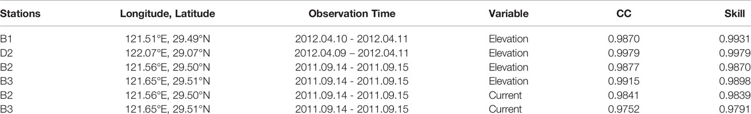
Table 1 Information of observation stations (B1, D2, B2 and B3), the correlation coefficient (CC), and the skill assessment parameter (Skill) of the elevation and current validations.

FIGURE 2

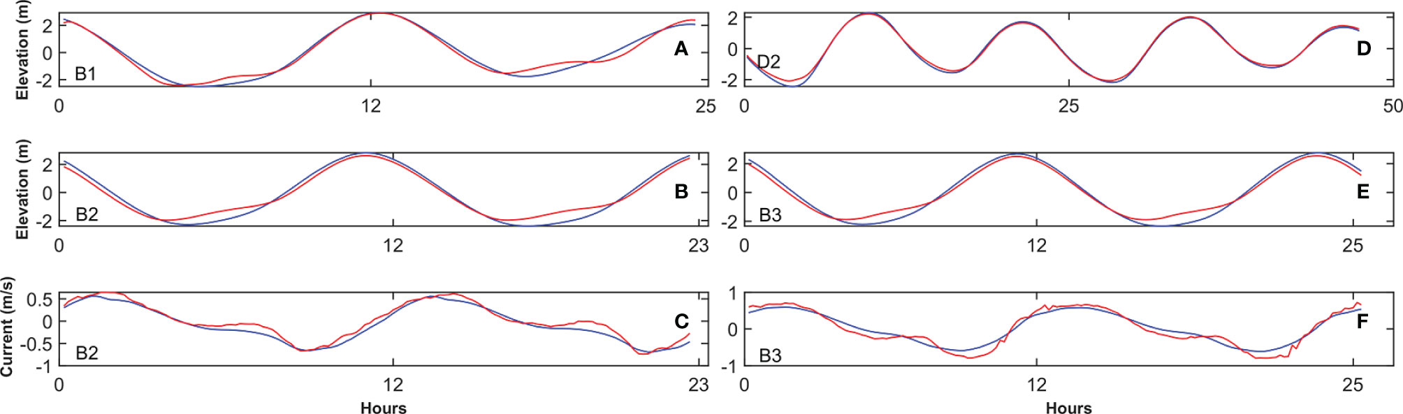
Figure 2 Comparisons between the observed (red line) and model (blue line) elevations and currents at four stations. Hourly time series of elevations at stations (A) B1, (B) B2, (D) D2 and (E) B3. Hourly time series of currents at stations (C) B2 and (F) B3.

To further evaluate the model performance, two statistical parameters including the correlation coefficient (CC) and Willmott Skill score (Willmott, 1981) are calculated, as follows:

$\begin{array}{ll}CC=\frac{{\sum }_{i=1}^N\left(o{b}_i-\overline{ob}\right)\left(m{o}_i-\overline{mo}\right)}{\sqrt{{\sum }_{i=1}^N{\left(o{b}_i-\overline{ob}\right)}^2{\sum }_{i=1}^N{\left(m{o}_i-\overline{mo}\right)}^2}},& (21)\end{array}$

$\begin{array}{ll}Skill=1-\frac{{\sum }_{i=1}^N{\left(o{b}_i-m{o}_i\right)}^2}{{\sum }_{i=1}^N{\left(\left|m{o}_i-\overline{ob}\right|+\left|o{b}_i-\overline{ob}\right|\right)}^2},& (22)\end{array}$

where ob_i and mo_iare the observation and model data, respectively, $\overline{ob}$ and $\overline{mo}$ denote the temporal average, respectively, and the N represents the number of observations. Table 1 shows the validation results of the model performance at four stations. The correlation coefficients are higher than 0.9752 and all Skill cores are bigger than 0.9791. The result indicates that the model can perform reasonably well.

The second task is a comparison between the residual current calculated by the model and that reported in previous works and derived from drifter data. The model is forced only by the M₂ tidal constituent, thus matching the result in Xu et al. (2016). The structure of the LRV has two branches—a branch flowing from the northern region of the Niubi Channel to the southern region of the Fodu Channel and another branch flowing from the northern region of the Fodu Channel to the southern region of the Niubi Channel in the outer Xiangshan Bay (Figure 3); these results are consistent with those noted in Xu et al. (2016). The LRV flows inside and outside from the north and south of the inner Xiangshan Bay, respectively (Figure 3). When the model is forced by multi-frequency tide and the temporally constant density gradient, the ERV has similar results to that in Wan et al. (2015). The results show a laterally sheared structure with inflow in the middle areas and outflow over two shoals from the surface layer to the bottom layer at the head of the inner Xiangshan Bay, and a gravitational circulation in the region between the middle and mouth of the inner Xiangshan Bay; in the outer Xiangshan Bay, the ERV flows inward from Fodu Channel and outward from the Niubi Channel (Figures 6A–C). Under the consideration of multi-frequency tide and the temporally constant density gradient, the LRV is seaward in the surface layer at the head of the inner Xiangshan Bay (Figure 4A), the same as that calculated based on drifter data (Sheng et al., 2022).

FIGURE 3

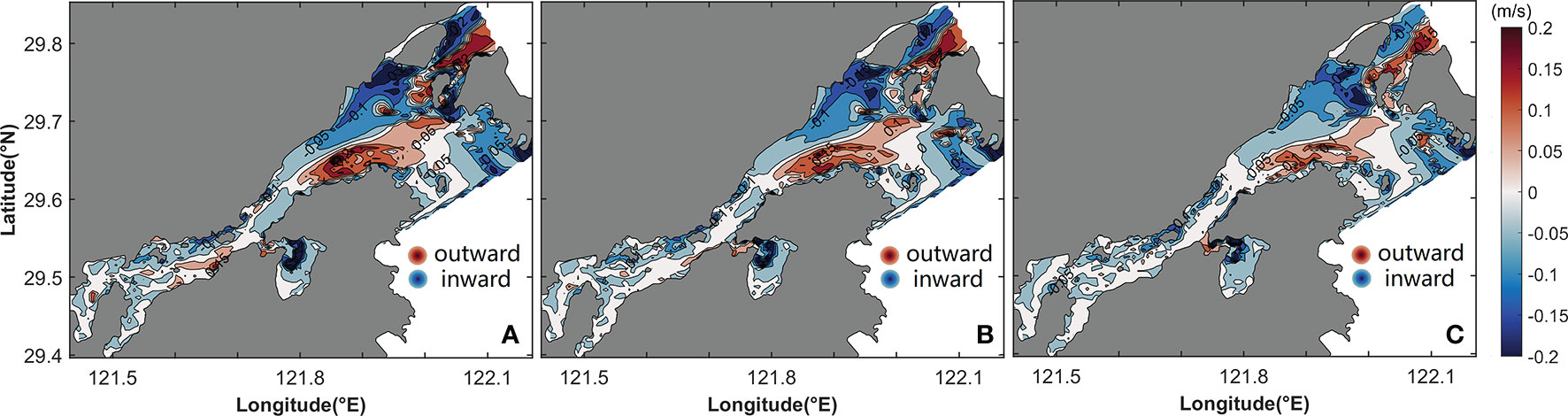
Figure 3 Horizontal distribution of the LRV for M₂ tidal constituent in the (A) surface, (B) middle, and (C) bottom layers. The shaded area and contours represent flow variation.

FIGURE 4

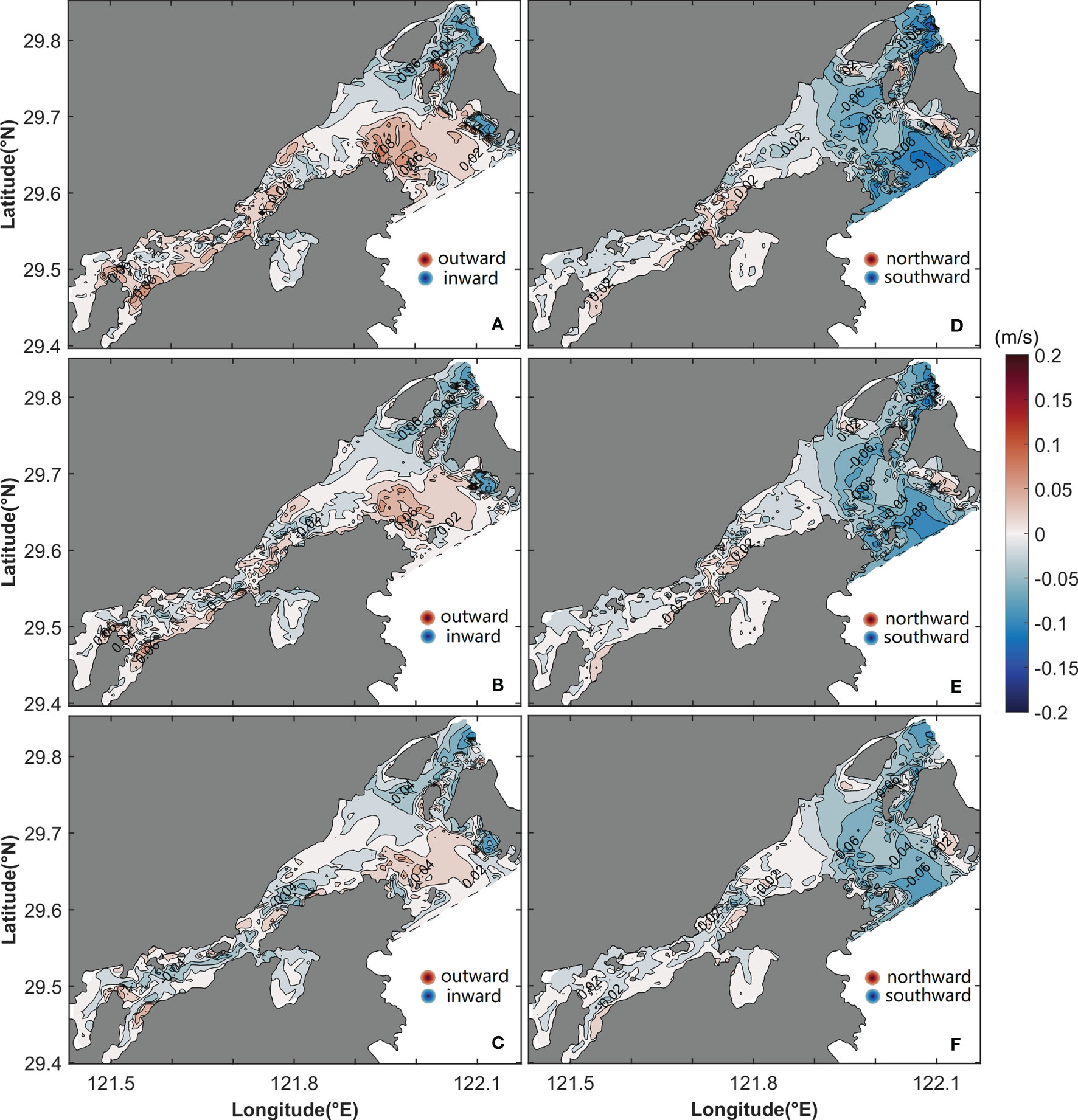
Figure 4 Horizontal distribution of u_L (A–C) and v_L (D–F) for multi-frequency tide in the (A, D) surface, (B, E) middle, and (C, F) bottom layers. The shaded area and contours represent flow variation.

3 Results

3.1 Structure of the LRV and ERV

When the temporally constant density gradient and multi-frequency tide are considered, the horizontal distributions of u_L in the surface, middle, and bottom layers are as shown in Figures 4A–C. In the outer Xiangshan Bay, u_L has the same pattern from the surface layer to the bottom layer, with inflow in the Fodu Channel and outflow in the Niubi Channel. The magnitude of u_L decreases slightly from the surface layer to the bottom layer in the outer Xiangshan Bay. u_L has the greatest value on the northern bank of the Fodu Channel and the southern bank of the Niubi Channel, with values of −0.06 m/s and 0.08 m/s, respectively. In the inner Xiangshan Bay, u_L shows a gravitational circulation with inflow in the bottom layer and outflow in the surface layer; in the middle layer, the LRV flows inward from the deep channel and outward from both shoals. In the inner Xiangshan Bay, u_L has a maximum value in the range 0.04 m/s–0.06 m/s. The horizontal pattern of v_L in Xiangshan Bay is shown in Figures 4D–F. In the outer Xiangshan Bay, v_L is negative, indicating a flow toward the southern bank. In the Niubi Channel, the magnitude of v_L decreases from 0.1 m/s in the surface layer to 0.06 m/s in the bottom layer. In the inner Xiangshan Bay, v_L flows southward on the northern bank and northwardon the southern bank, and the two flows meet in the deep channel. At the mouth of the inner Xiangshan Bay, a two-layer structure of v_L is present, with a northward flow in the lower layer and a southward flow in the upper layer. The magnitude of v_L reaches a maximum value of 0.04 m/s in the inner Xiangshan Bay, which is approximately half the value in the outer Xiangshan Bay.

The vertical structures of u_L and v_L in four cross sections are shown in Figure 5. Significant differences in the pattern of the LRV are observed in the four cross sections. The cross section of the middle of the inner Xiangshan Bay has inflows in the middle areas and outflows on both sides (Figure 5A); the inflow increases with an increase in depth and peaks at a magnitude of 0.03 m/s, whereas the outflow decreases with an increase in depth and peaks in the upper layers of both sides. In the cross section of the mouth of the inner Xiangshan Bay, the LRV has a two-layer vertically sheared structure with inflows in the lower layers and outflows in the upper layers (Figure 5B). In the cross sections of the Niubi Channel and Fodu Channel, outflows with a maximum value of 0.04 m/s occupy the cross section of the Niubi Channel, except in some shoal areas, and inflows with a peak value of −0.06 m/s are present in the cross section of Fodu Channel (Figures 5C, D). The vertical structure of v_L in the four cross sections is shown in Figures 5E–H. In the cross section of the middle of the inner Xiangshan Bay, v_L flows northward on the southern bank and southward on the northern bank, and its magnitude decreases as the depth increases. A southward flow with a maximum value of −0.008 m/s exists in the surface layers, and a northward flow with a peak value of 0.006 m/s is present in the middle and lower layers of the cross section of the mouth of the inner Xiangshan Bay. In the cross sections of the Niubi Channel and Fodu Channel, the southward flow occupies all areas except some small areas; the peak value of -0.1 m/s is observed on the southern bank of the cross section of the Niubi Channel and the deep portion of the cross section of the Fodu Channel.

FIGURE 5

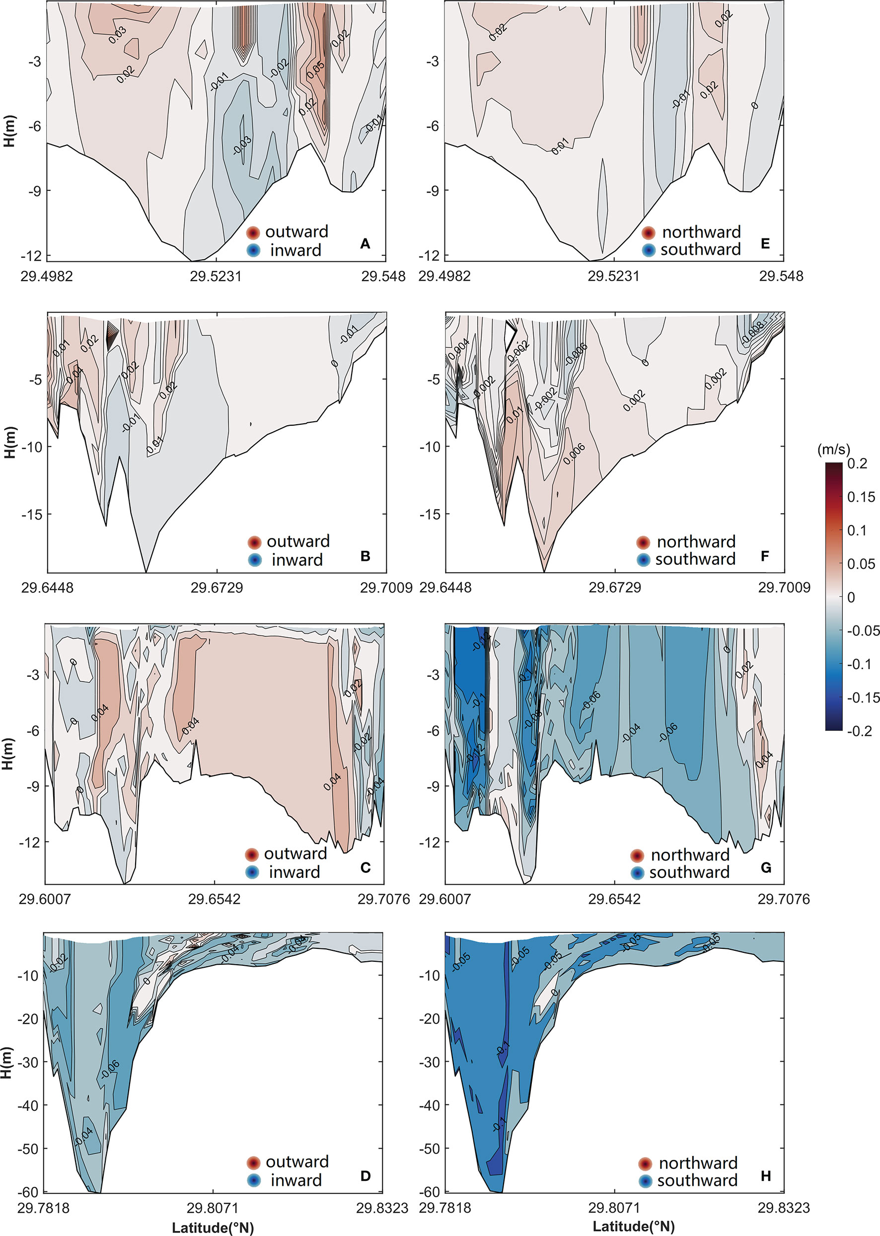
Figure 5 Vertical structure of u_L (A–D) and v_L (E–H) in (A, E) the cross section of the middle of the inner Xiangshan Bay, (B, F) the cross section of the mouth of the inner Xiangshan Bay, (C,G) the cross section of the Niubi Channel, and (D, H) the cross section of the Fodu Channel. The shaded area and contours represent flow variation. The locations of the four cross sections are shown in Figure 1.

The horizontal distributions of u_E and v_E are shown in Figure 6. The u_E in the outer bay flows in through the Fodu Channel and out from the Niubi Channel, showing the same pattern as u_L; the difference is that u_E has a greater magnitude than u_L. In the Niubi Channel, u_E peaks on both sides with a magnitude of 0.1 m/s, whereas in the Fodu Channel, the peak u_E value of −0.11 m/s appears in the deep part of the channel (Figure 6A). In the inner Xiangshan Bay, u_E flows inward through the deep channel and outward from both sides and the magnitude of u_E decreases from the surface layer to the bottom layer, with a maximum value of 0.1 m/s at the surface on both sides of the inner Xiangshan Bay (Figures 6A–C). The v_E flows nearly southward from the surface layer to the bottom layer in the entire bay, except in some shoal areas of the inner Xiangshan Bay (Figures 6D–F). The v_E decreases from the surface layer to the bottom layer, and the peak values appear in the surface layer, with a magnitude of 0.13 m/s in the inner Xiangshan Bay and 0.14 m/s in the outer Xiangshan Bay.

FIGURE 6

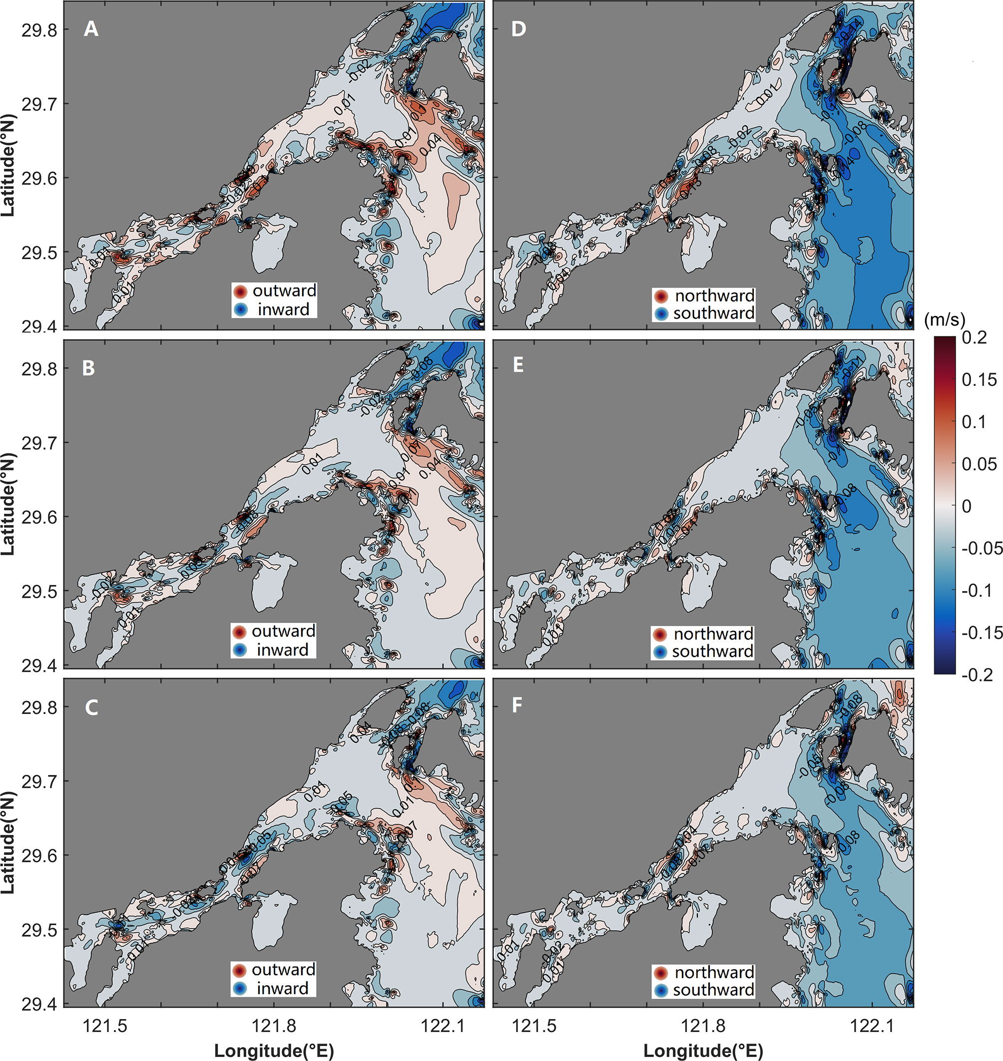
Figure 6 Horizontal distribution of u_E (A–C) and v_E (D–F) in the (A, D) surface, (B, E) middle, and (C, F) bottom layers. The shaded area and contours represent flow variation.

The vertical structures of u_E and v_E are shown in Figure 7. The u_E shows obvious differences in the cross section of the mouth of the inner Xiangshan Bay (Figure 7B)—with inflow in the channel and outflow on both sides—when compared with the two-layer structure of the LRV in the same cross section (Figure 5B). In the other three cross sections, u_E has the same structure as u_L; however, their magnitudes, especially in the cross sections of the Niubi Channel and the Fodu Channel, are significantly different. The maximum value of u_E in the two cross sections is 2–3 times that of u_L. The vertical structure of v_E is different from that of v_L, especially in the cross sections of the middle and the mouth of the inner Xiangshan Bay. The v_E flows southward in the two cross sections except for some bank areas (Figures 7E, F), thus differing from the northward flow of v_L in most areas of the cross section of the middle of the inner Xiangshan Bay (Figure 5E) and the two-layer structure of v_L in the cross section of the mouth of the inner Xiangshan Bay (Figure 5F). The peak value of v_E is 1–2 times greater than that of v_L in the two cross sections. In the cross sections of the Niubi Channel and the Fodu Channel, the structures of v_E are approximately the same as those of v_L; however, their magnitudes are significantly different (Figures 7G, H).

FIGURE 7

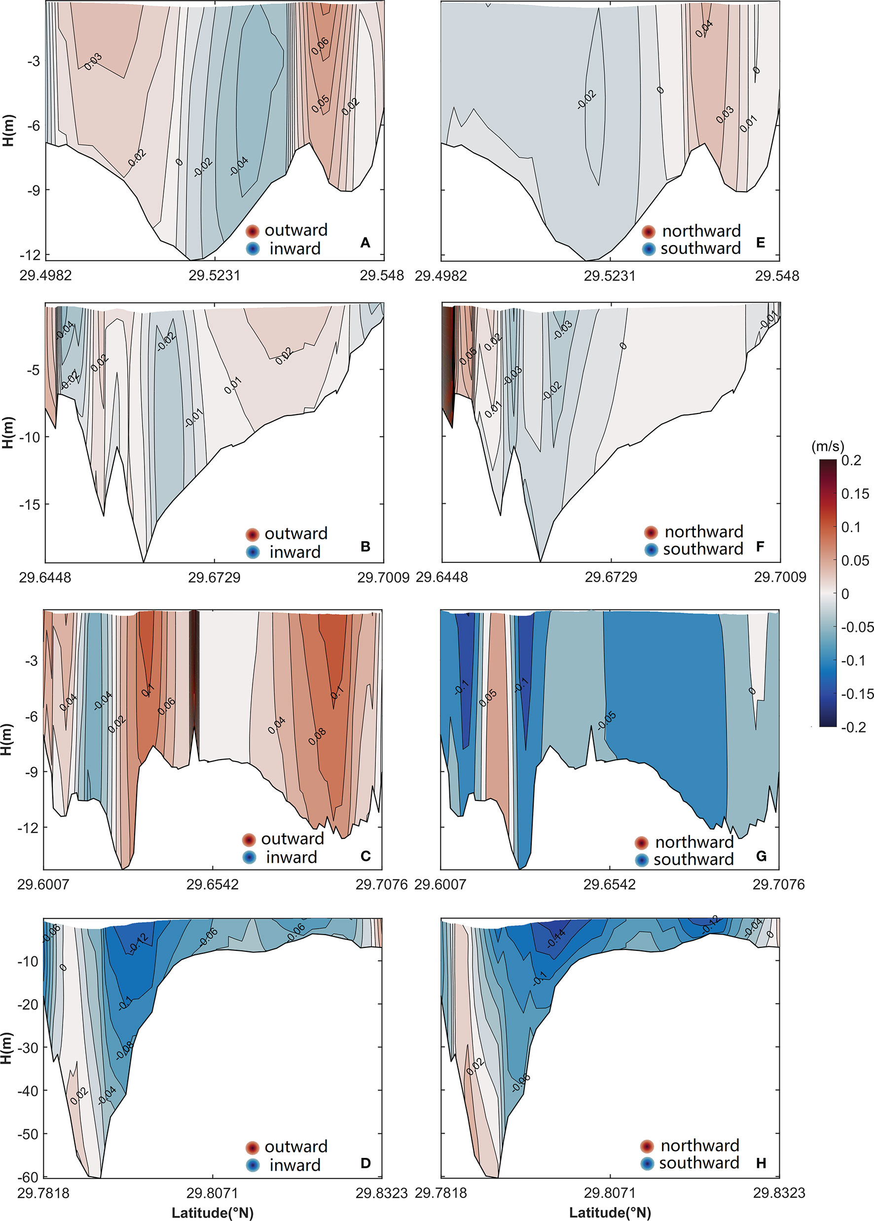
Figure 7 Vertical structure of u_E (A–D) and v_E (E–H) in (A, E) the cross section of the middle of the inner Xiangshan Bay, (B, F) the cross section of the mouth of the inner Xiangshan Bay, (C, G) the cross section of the Niubi Channel, and (D, H) the cross section of the Fodu Channel. The shaded area and contours represent flow variation. The locations of the four cross sections are shown in Figure 1.

Overall, there are obvious differences between the structures of the ERV and the LRV in the inner Xiangshan Bay, and their magnitudes are significant not only in the inner Xiangshan Bay but also in the outer Xiangshan Bay. The dynamic mechanisms of the ERV and LRV considering density gradient constant in time are notably different and are analyzed below.

3.2 Decomposition of the ERV and LRV

3.2.1 Components of the ERV

Based on the decomposition method for the ERV presented in Section 2.1.1, the longitudinal and lateral ERV are decomposed into acceleration components u_Eac and v_Eac, nonlinear advection components u_Ead and v_Ead, barotropic pressure gradient components u_Eba and v_Eba, density gradient components u_Egr and v_Egr, eddy viscosity components u_Etu and v_Etu, and horizontal diffusion components u_Eho and v_Eho.

The nonlinear advection component and barotropic pressure gradient component of ERV are greater than the components of ERV induced by other forces by one order of magnitude but the two components are reverse in structure (pictures are not included). The sum of u_Eac, u_Ead, and u_Eba in the four cross sections is shown in Figures 8A–D. The structure of the sum of these three components primarily determines the structure of the total u_E, except in some small areas. In the cross section of the middle of the inner Xiangshan Bay, the sum of u_Eac, u_Ead, and u_Eba shows a laterally sheared structure with inflow in the middle area and outflow on both sides (Figure 8A), which has the same pattern as that of the total u_E and is greater than total u_E in magnitude on the northern bank in the same cross section (Figure 7A). In the cross section of the mouth of the inner Xiangshan Bay, inflow exists in the middle area and on both sides, and outflow occupies the slope (Figure 8B), consistent with the pattern of the total u_E in the same cross section (Figure 7B). In the cross section of the Niubi Channel, the only difference is that the inflow area expands on the southern bank and in some small middle areas (Figure 8C), compared with the total u_E (Figure 7C). In the cross section of the Fodu Channel, landward flow dominates in most areas of the cross section except in the upper layers of the southern slope (Figure 8D); this result matches the pattern of the total u_E (Figure 7D). The sum of v_Eac, v_Ead, and v_Eba is shown in Figures 8E–H. The pattern of flow induced by the collective effects of the three components dominates the structure of the total v_E even though the magnitude is not entirely consistent. The sum of v_Eac, v_Ead, and v_Eba flows northward from the northern slope and southward from the residual areas in the cross section of the middle of the inner Xiangshan Bay (Figure 8E); this result is nearly the same as the pattern of the total v_E (Figure 7E), except that the northward flow area of the total v_E expands on the northern side. Northward flow appears on the southern sides and the lower layers of the middle areas, and southward flow is present in the residual areas of the cross section of the mouth of the inner Xiangshan Bay (Figure 8F); these results are highly consistent with those of the total v_E(Figure 7F). In the cross section of the Niubi Channel, northward flow occupies a small area on the southern bank whereas southward flow dominates the cross-sectional area (Figure 8G); this result closely matches the pattern of the total v_E (Figure 7G). In the cross section of the Fodu Channel, the flow is southward in the entire cross section except for a few scattered areas where the flow is northward (Figure 8H); this result slightly differs from that of the total v_E in which northward flow is only distributed on the southern bank (Figure 7H). For both the longitudinal and lateral ERV, the magnitude of the sum of the three components is slightly greater than the total ERV in the four cross sections, indicating that the components of ERV induced by other forces play a secondary role in shaping the total ERV.

FIGURE 8

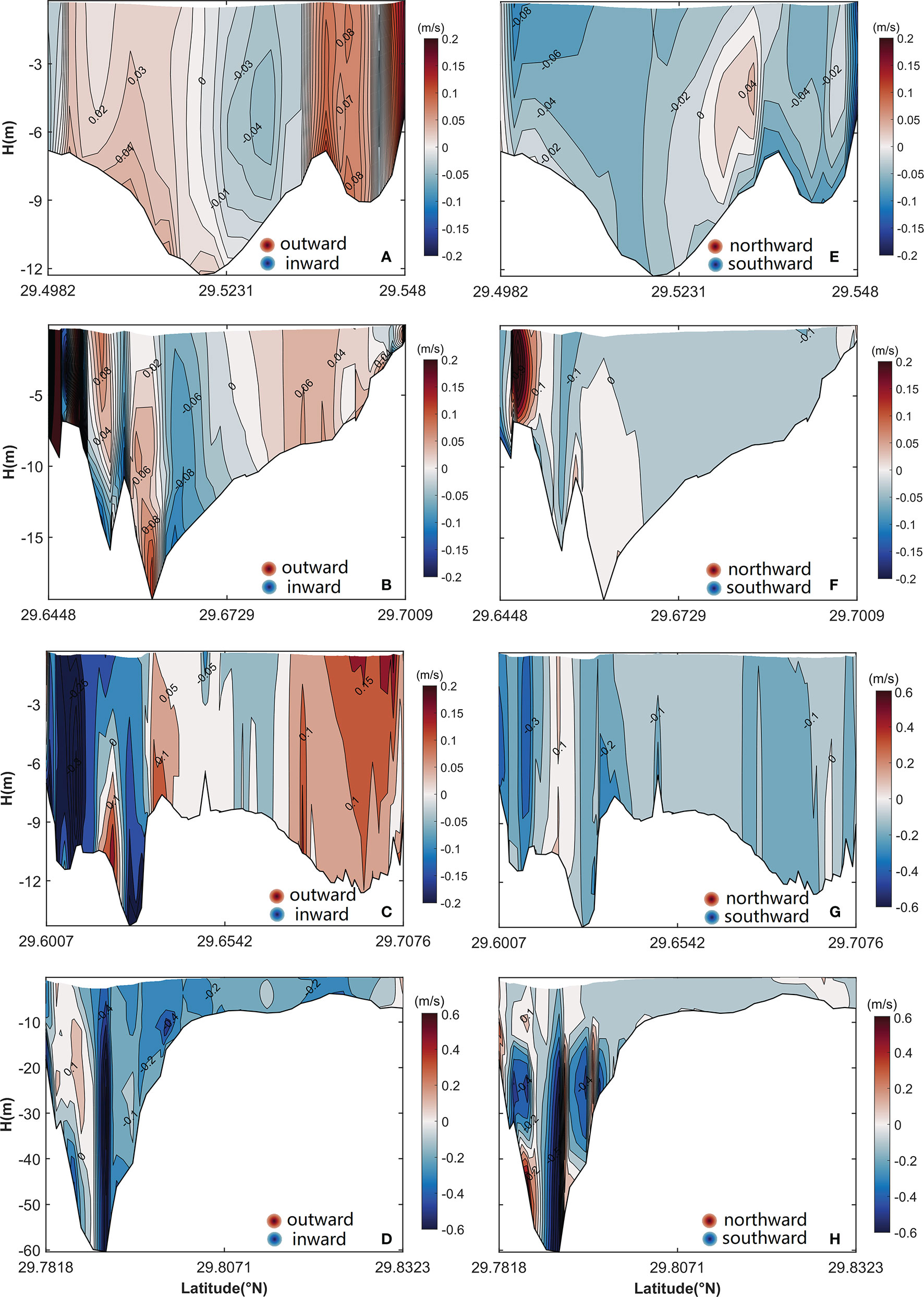
Figure 8 The vertical structure of the sum of the Longitudinal (A–D) and lateral (E–H) acceleration, nonlinear advection, and barotropic pressure gradient components of ERV in (A, E) the cross section of the middle of the inner Xiangshan Bay, (B, F) the cross section of the mouth of the inner Xiangshan Bay, (C, G) the cross section of the Niubi Channel, and (D, H) the cross section of the Fodu Channel. The shaded area and contours represent flow variation. The locations of the four cross sections are shown in Figure 1.

3.2.2 Components of the LRV

Based on the decomposition method for the LRV in Section 2.1.2, the longitudinal and lateral LRV are decomposed into acceleration components u_Lac and v_Lac, nonlinear advection components u_Lad and v_Lad, barotropic pressure gradient components u_Lba and v_Lba, density gradient components u_Lgr and v_Lgr, eddy viscosity components u_Ltu and v_Ltu, and horizontal diffusion components u_Lho and v_Lho.

The barotropic pressure gradient component u_Lba and density gradient component u_Lgr are shown in Figure 9. The u_Lba is depth-independent with the same pattern and magnitude from the surface layer to the bottom layer (Figures 9A–C). Inflow is dominant in the outer Xiangshan Bay, except on the southern bank of the Fodu Channel and the northeastern side of the Niubi Channel, where the outflow is present. At the mouth of the inner Xiangshan Bay, u_Lba shows inflow in the middle area, with outflow on both sides. In the inner Xiangshan Bay, outflow occupies all areas except the northern bank of the head of the inner Xiangshan Bay.

FIGURE 9

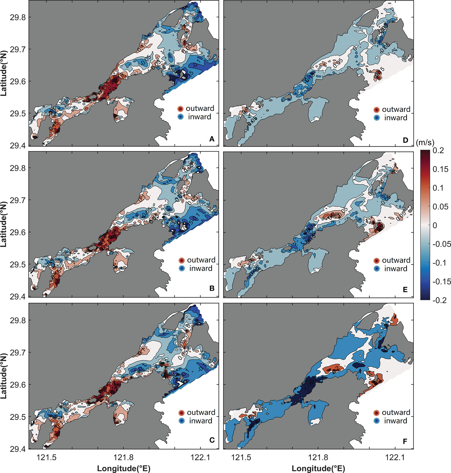
Figure 9 Horizontal distribution of the longitudinal barotropic pressure gradient component (u_Lba; A–C) and density gradient component of LRV (u_Lgr; D–F) in the surface (A, D), middle (B, E), and bottom (C, F) layers. The shaded area and contours represent flow variation.

The density gradient component u_Lgr has the same structure but has an increasing intensity from the surface layer to the bottom layer (Figures 9D–F). The structure of u_Lgr is the reverse of that of u_Lba. In the outer Xiangshan Bay, inflow dominates on the southern bank and outflow dominates on the northern bank in the Fodu Channel, and inflow and outflow occupy the inner and outer areas of the Niubi Channel, respectively, nearly reverse to the pattern of u_Lba. At the mouth of the inner Xiangshan Bay, inflow on the two sides encloses outflow; and inflow dominates in the inner Xiangshan Bay except on the northern side of the head of the inner Xiangshan Bay; this structure is the reverse of the corresponding structure for u_Lba. Closer to the bottom layer, the density gradient drives a flow that is more intense than that at the surface, with the peak value varying from -0.15 m/s to -0.2 m/s.

The barotropic pressure gradient component v_Lba shows the same pattern from the surface layer to the bottom layer and drives the water flow southward (Figures 10A–C). The v_Lba attains a maximum value of -0.2 m/s in the inner Xiangshan Bay. The structure of the density gradient component v_Lgr is the reverse of that of v_Lba, except in some small areas, forcing the water to flow northward. The v_Lgr has the same pattern across layers; however, its magnitude increases from the surface layer to the bottom layer (Figures 10D–F) and attains a maximum value of approximately 0.25 m/s in the bottom layer (Figure 10F).

FIGURE 10

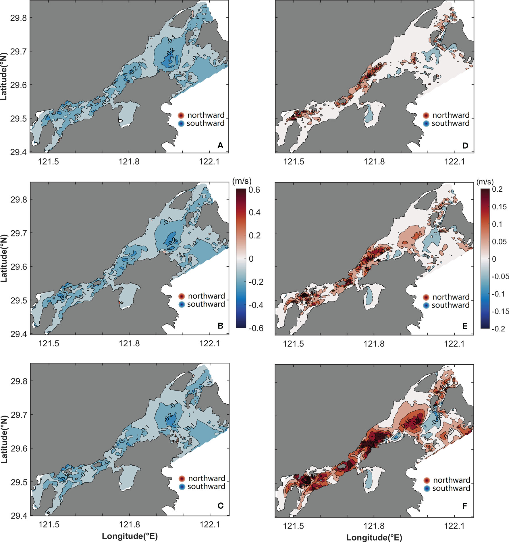
Figure 10 Horizontal distribution of the lateral barotropic pressure gradient component (v_Lba; A–C) and density gradient component (v_Lgr; D–F) in the surface (A, D), middle (B, E), and bottom (C, F) layers. The shaded area and contours represent flow variation.

In the surface layer, the eddy viscosity component u_Ltu flows seaward in the Niubi Channel, except in the northern area, and has a maximum value of 0.13 m/s at the mouth of the Niubi Channel. In the Fodu Channel, inflow and outflow are distributed on the southern and northern banks, respectively. In the inner Xiangshan Bay, inflow is dominant, with a maximum value of -0.08 m/s (Figure 11A). The inflow area in the outer Xiangshan Bay and outflow area in the inner Xiangshan Bay expand, and the magnitude of u_Ltu decreases from the surface layer to the bottom layer (Figures 11A–C). The eddy viscosity component v_Ltu flows northward from the surface layer and southward from the bottom layer in the inner Xiangshan Bay (Figures 11D, F). Southward flow exists in the Fodu Channel and northward flow dominates in the Niubi Channel except in the bottom layers on the two banks (Figures 11D–F).

FIGURE 11

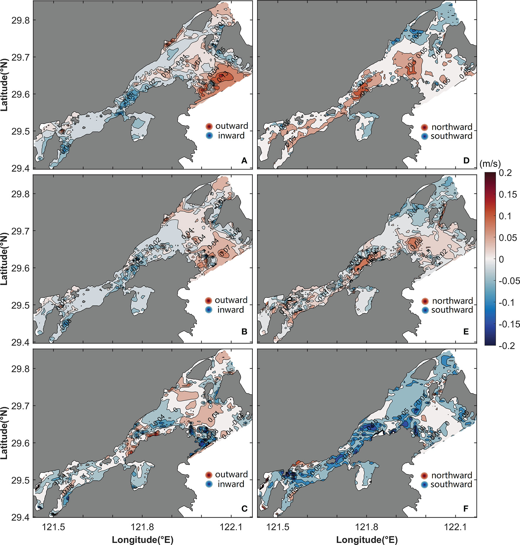
Figure 11 Horizontal distribution of the longitudinal (u_Ltu; A–C) and lateral (v_Ltu; D–E) components of eddy viscosity in the surface (A, D), middle (B, E), and bottom (C, F) layers. The shaded area and contours represent flow variation.

The vertical structure of u_Ltu is shown in Figures 12A–D. The u_Ltu is laterally sheared, with the outward flow in the channel and inward flow on both banks in the cross section of the middle of the inner Xiangshan Bay (Figure 12A). In the cross section of the mouth of the inner Xiangshan Bay, u_Ltu is vertically sheared, with outflow and inflow in the upper layer and lower layer, respectively (Figure 12B). Outflow is present in all areas of the cross section of the Niubi Channel except for a small inflow area on the northern bank (Figure 12C), which dominates the structure of the total u_L (Figure 5C). In the cross section of the Fodu Channel, the inflow area is distributed in the upper layers of the channel, and the outflow area is scattered on both banks (Figure 12D).

FIGURE 12

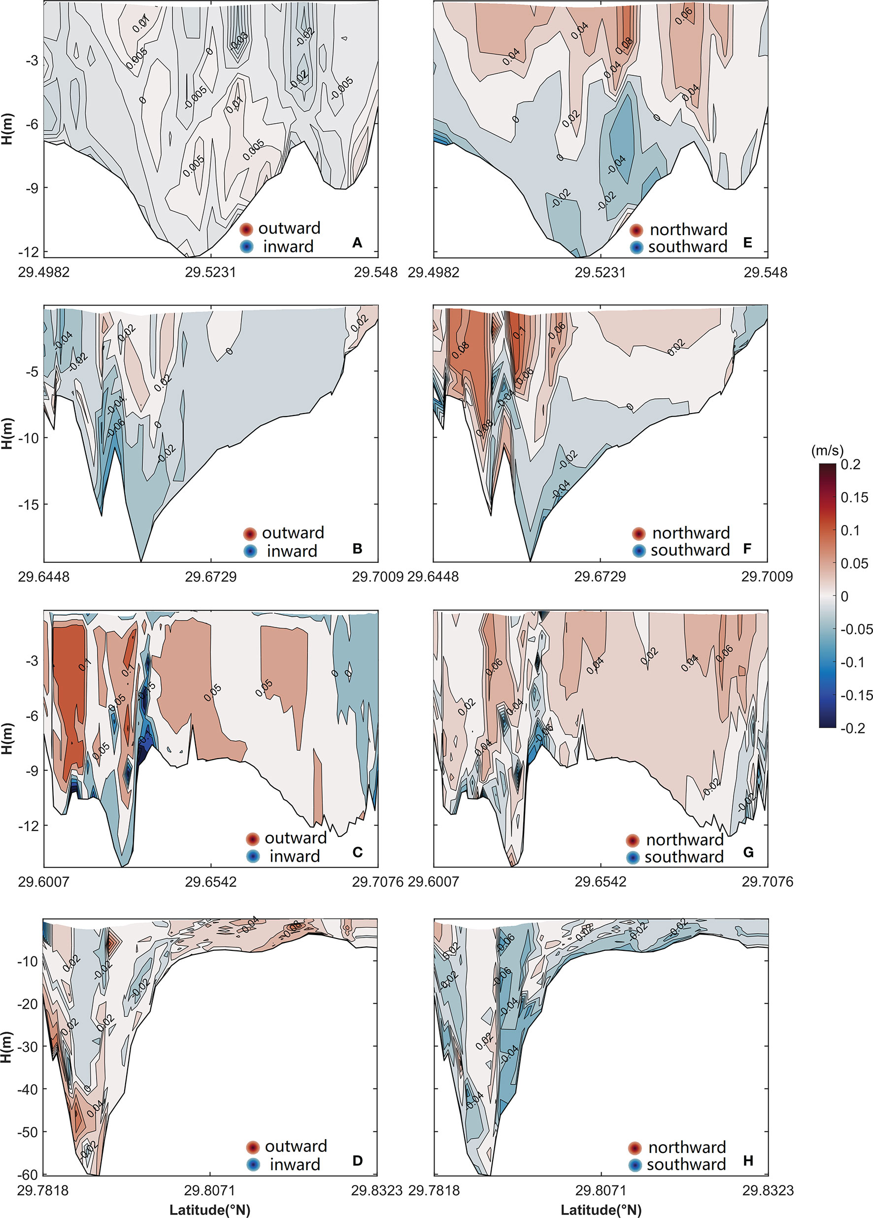
Figure 12 Vertical structure of the longitudinal (u_Ltu; B–E) and lateral (v_Ltu; E–H) components of eddy viscosity in (A, E) the cross section of the middle of the inner Xiangshan Bay, (B, F) the cross section of the mouth of the inner Xiangshan Bay, (C, G) the cross section of the Niubi Channel, and (D, H) the cross section of the Fodu Channel. The shaded area and contours represent flow variation. The locations of the four cross sections are shown in Figure 1.

The eddy viscosity component v_Ltu is a two-layer structure with the northward flow in the upper layer and southward flow in the lower layer in the cross sections of the middle and the mouth of the inner Xiangshan Bay (Figures 12E, F). The v_Ltu has a unidirectional northward flow in the cross section of the Niubi Channel except in some small areas (Figure 12G) and a laterally sheared structure in the cross section of the Fodu Channel, with the northward flow in the channel and southward flow on both banks (Figure 12H).

The sum of the longitudinal acceleration component u_Lac and nonlinear advection component u_Lad is landward in the inner Xiangshan Bay and the Fodu Channel (Figures 13A–C), and the flow is seaward in the Niubi Channel. The sum of the acceleration component v_Lac and the nonlinear advection component v_Lad results in a unidirectional northward flow in the Xiangshan Bay except for southward flow in the outer area and on both banks of the Niubi Channel (Figures 13D–F).

FIGURE 13

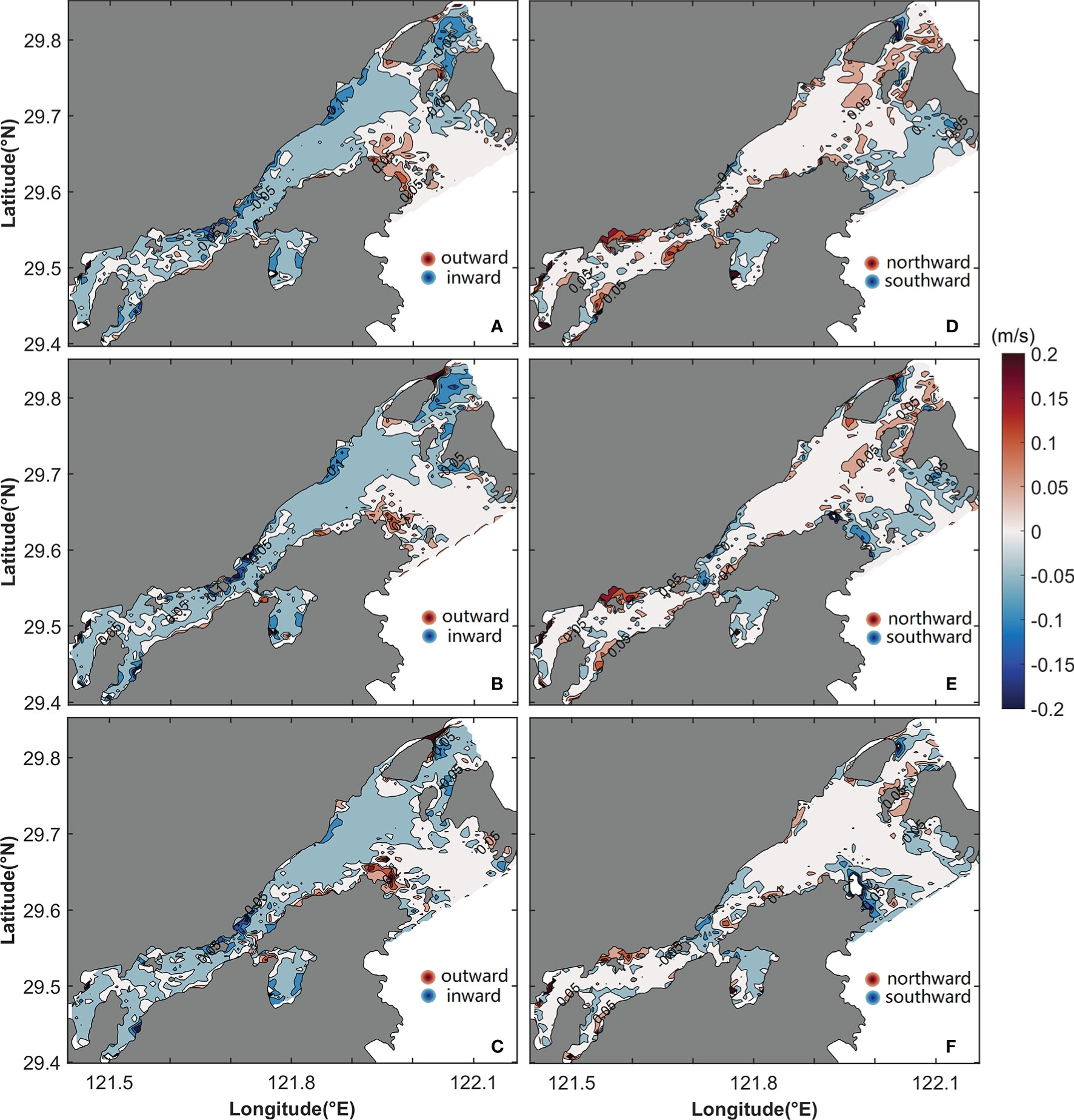
Figure 13 Horizontal distribution of the sum of the longitudinal (A–C) and lateral (D–F) acceleration and the nonlinear advection components of LRV in the surface (A, D), middle (B, E), and bottom (C, F) layers. The shaded area and contours represent flow variation.

The contribution of the horizontal diffusion components u_Lho and v_Lho to the total LRV is smaller than the components of LRV induced by other forces (pictures are not included).

The total u_L in the Fodu Channel flows inward, which is mainly determined by the sum of the acceleration component u_Lac and nonlinear advection component u_Lad. In the Niubi Channel, the eddy viscosity-induced outflow dominates the total u_L. At the surface of the inner Xiangshan Bay, the barotropic pressure gradient component u_Lba is the main contributor to the outflow. At the bottom of the inner Xiangshan Bay, the inflow is dominated by the density gradient component u_Lgr. The total v_L in the Fodu Channel and Niubi Channel is mainly influenced by the barotropic pressure gradient-induced southward flow. In the inner Xiangshan Bay, the total v_L is determined by the collective effect of the components of LRV induced by all of the forces.

The total longitudinal LRV of the six components derived through decomposition methods (Figure 14) has a transverse structure that closely matches the structure obtained through the direct use of tracking methods (Figures 5A–D). There is a slight difference in the magnitudes obtained using the two methods; this difference is attributable to the spatial and temporal resolution of tracking and interpolation. The results of the comparison demonstrate the self-consistency of the decomposition methods.

FIGURE 14

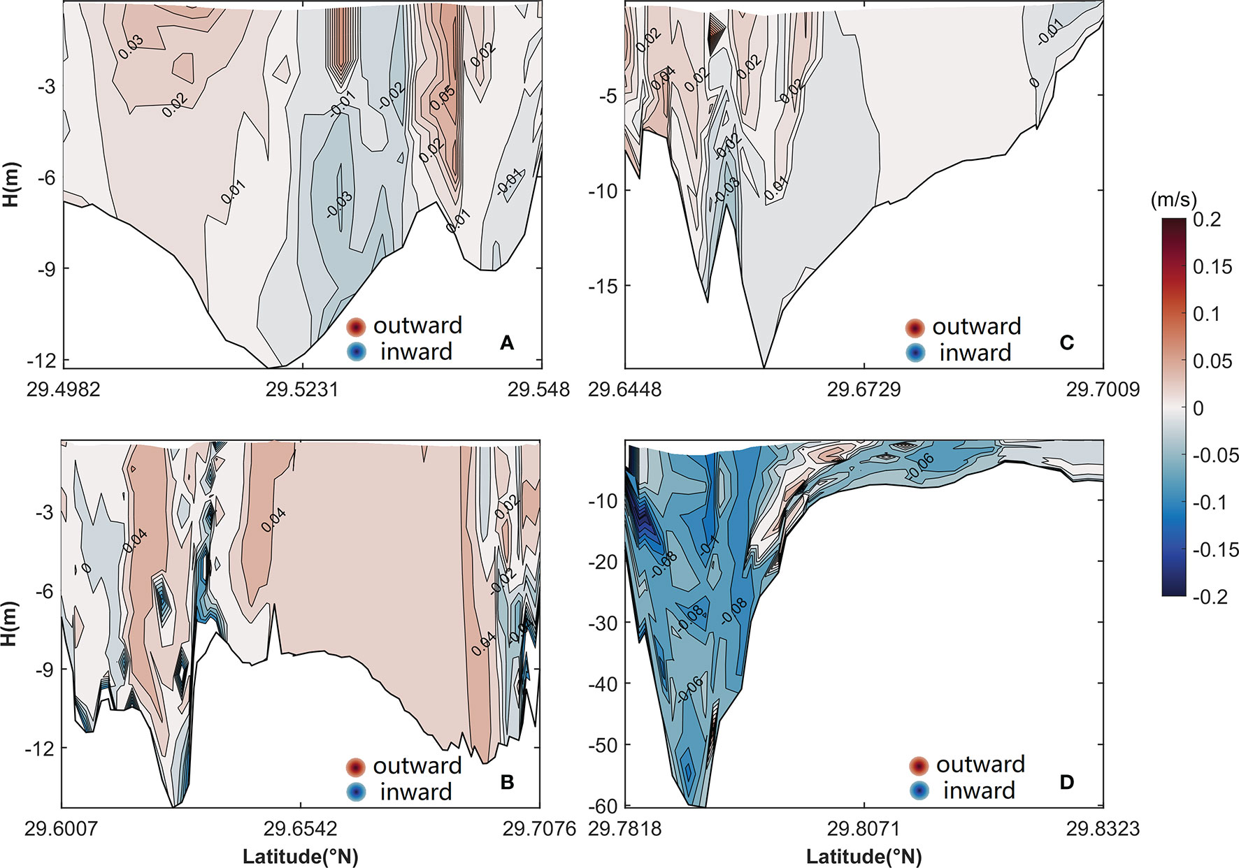
Figure 14 Vertical structure of the sum of u_Lac, u_Lad, u_Lba, u_Lgr, u_Ltu, and u_Lho in (A) the cross section of the middle of the inner Xiangshan Bay, (B) the cross section of the mouth of the inner Xiangshan Bay, (C) the cross section of the Niubi Channel, and (D) the cross section of the Fodu Channel. The shaded area and contours represent flow variation. The locations of the four cross sections are shown in Figure 1.

3.3 Intensity of Each Component of the ERV and LRV

The relative importance of the horizontal density gradient and the eddy viscosity term is measured by a dimensionless parameter defined as the modified horizontal Richardson number (RI) (Burchard and Hetland, 2010):

$\begin{array}{ll}RI=\frac{{\partial }_{x}b{H}^2}{u_{max}^2},& (23)\end{array}$

where ∂_xb is the tidally averaged horizontal density gradient, u_max is the absolute maximum velocity, and H is the depth of still water.

To determine the relative importance of the component of residual velocity induced by each force, the mean of their absolute values in the cross section is defined as follows [similar to Equation (29) in Burchard and Hetland (2010) in the vertical profile]:

$\begin{array}{ll}M(·)=\frac{1}{B}{\displaystyle \int abs(·)dB,}& (24)\end{array}$

where abs represents the absolute value function. The symbol · can be replaced with each component of the ERV and LRV. B represents the transect area. The contribution ratio of each component to the total residual velocity R(·) is defined as follows:

$\begin{array}{ll}R(·)=\frac{M(·)}{sum\left(M(·)\right)}.& (25)\end{array}$

3.3.1 Relative Contribution of Each Component to the ERV

In the Eulerian-averaged condition, the nonlinear advection component of ERV has the same magnitude as the barotropic pressure gradient component. They account for 30%–40% each of the total ERV. The components of ERV induced by other forces have a small contribution ratio to the total ERV and influence the total ERV differently in the four cross sections.

In the cross section of the middle of the inner Xiangshan Bay, the longitudinal acceleration component, density gradient component, eddy viscosity component, and horizontal diffusion component of ERV [R(u_Eac),R(u_Egr),R(u_Etu), and R(u_Eho) in Table 2a] each account for approximately 4%–5% of the total ERV. In the same cross section, the lateral acceleration component and horizontal diffusion component of ERV account for 3% and 2% of the total ERV [R(v_Eac) and R(v_Eho) in Table 2a], respectively, which are 1/3–1/4 of the density gradient component and eddy viscosity component of ERV [R(v_Egr) and R(v_Etu) in Table 2a].

TABLE 2

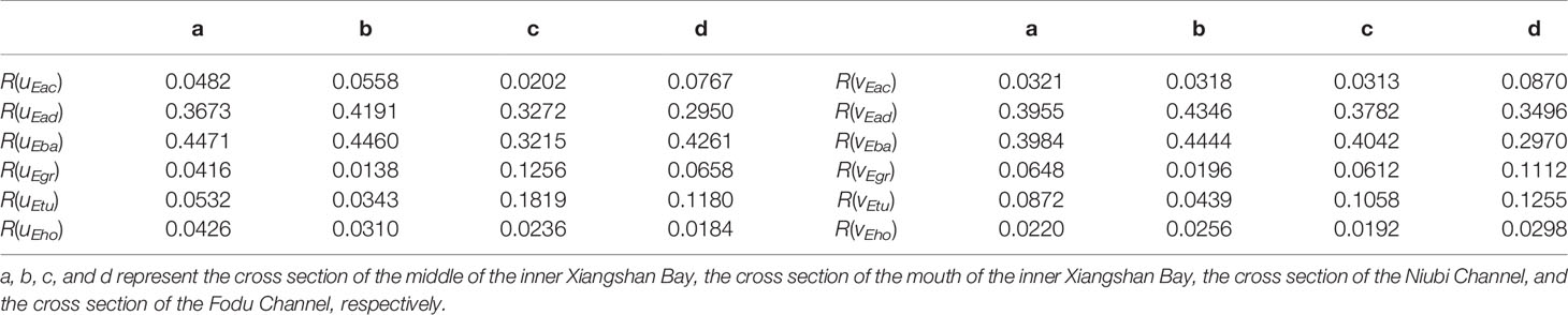
Table 2 Contribution ratio of each component to the total ERV.

In the cross section of the mouth of the inner Xiangshan Bay, the longitudinal acceleration component of ERV accounts for 5.58% of the total ERV [R(u_Eac) in Table 2b]; the longitudinal eddy viscosity component and horizontal diffusion component of ERV have the nearly same contributing percentage [R(u_Etu) and R(u_Eho) in Table 2b]. In the same cross section, the contribution ratios of the lateral acceleration component and horizontal diffusion component of ERV are similar to those in the cross section of the middle of the inner Xiangshan Bay [R(v_Eac) and R(v_Eho) in Table 2b]; however, the difference is that the lateral density gradient component of ERV is the smallest [1.96%; R(v_Egr) in Table 2b] and is approximately half the size of the eddy viscosity component of ERV [4.39%; R(v_Etu) in Table 2b].

In the cross sections of the Niubi Channel and Fodu Channel, the eddy viscosity component of ERV accounts for more than 10% of the total ERV and makes the third highest contribution to the total ERV [R(u_Etu) and R(v_Etu) in Tables 2c,d], which is greater than the contribution of the density gradient component of ERV [R(u_Egr) and R(v_Egr) in Tables 2c,d]. The acceleration component of ERV has a larger contributing ratio in the cross section of the Fodu Channel than in other cross sections [R(u_Eac) and R(v_Eac) in Table 2d].

For a comparison with the results from previous studies (Burchard and Hetland, 2010; Burchard et al., 2011), the relationship between the eddy viscosity component and the density gradient component of ERV is analyzed; it is observed that the ratio between them differs for different values of RI (Table 3). The eddy viscosity component of ERV is more than two times the density gradient component of ERV when RI is 1.8 × 10⁴ (Table 3b), which is highly consistent with the results in Burchard and Hetland (2010), and the ratio of the eddy viscosity component of ERV to the density gradient component of ERV decreases as RI increases, indicating that the relative contribution of the density gradient component of ERV increases, which matches the results in Burchard et al. (2011).

TABLE 3

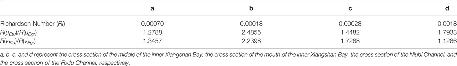
Table 3 The horizontal Richardson number (RI) and the ratio of the eddy viscosity component of ERV to the density gradient component of ERV.

3.3.2 Relative Contribution of Each Component to the LRV

The acceleration component, nonlinear advection component, and barotropic pressure gradient component of LRV are the three dominant components. The barotropic pressure gradient component of LRV [R(u_Lba) and R(v_Lba) in Table 4] is the greatest contributor; it is approximately 2–4 times the density gradient component of LRV [R(u_Lgr) and R(v_Lgr) in Table 4] in the four cross sections. The acceleration component of LRV [R(u_Lac) and R(v_Lac) in Table 4] has the same magnitude as the nonlinear advection component of LRV [R(u_Lad) and R(v_Lad) in Table 4], which is different from the case of ERV, in which the acceleration component of ERV [R(u_Eac) and R(v_Eac) in Table 2] is one order of magnitude smaller than the nonlinear advection component of ERV [R(u_Ead) and R(v_Ead) in Table 2].

TABLE 4

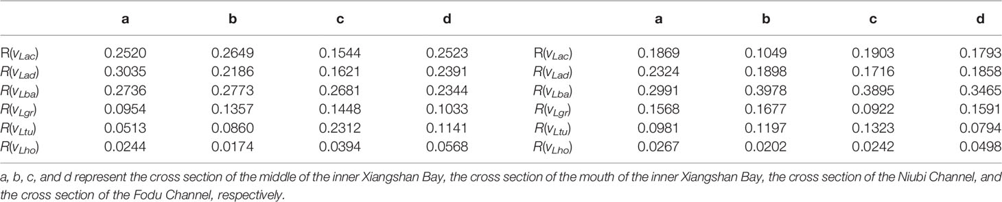
Table 4 Contribution ratio of each component to the total LRV.

The longitudinal eddy viscosity component of LRV is the second greatest contributor to the total LRV in the cross section of the Niubi Channel [R(u_Ltu) in Table 4c]; it is approximately 1.6 times the density gradient component of LRV [R(u_Ltu)/R(u_Lgr) in Table 5c]. However, in the other three cross sections, the longitudinal eddy viscosity component of LRV has a relatively small contributing ratio [R(u_Ltu) in Tables 4a, b, d]. The lateral eddy viscosity component of LRV is approximately 1.4 times the density gradient component of LRV in the cross section of the Niubi Channel [R(v_Ltu)/R(v_Lgr) in Table 5c] and approximately 0.5 to 0.7 times the density gradient component of LRV in the cross sections of the middle and mouth of the inner Xiangshan Bay, and the Fodu Channel (R(v_Ltu)/R(v_Lgr) in Tables 5a, b, d).

TABLE 5

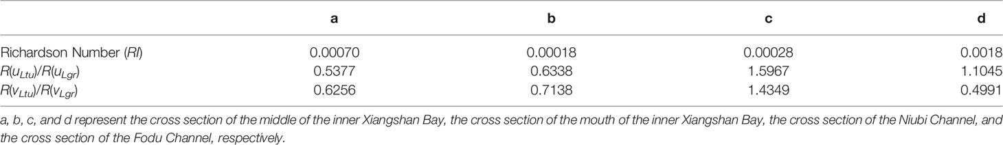
Table 5 The horizontal Richardson number (RI) and the ratio of the eddy viscosity component of LRV to the density gradient component of LRV.

The horizontal diffusion component of LRV is smaller than the components of LRV induced by the other forces; it accounts for 2%–5% of the total LRV, revealing that it is not a dominant component [R(u_Lho) and R(v_Lho) in Table 4)].

4 Discussion and Conclusions

In the Lagrangian-averaged approach, the decomposition method requires a high temporal resolution. In this study, results are analyzed when the time steps for the tracking algorithm are 10 min and 30 s, respectively. The results demonstrate that the difference in the trajectories is more pronounced as the integration time increases. The difference between the sum of the six components and the total LRV obtained through the direct use of tracking methods is notable, and the error is comparable to the actual value of the total LRV when the time step is 10 min. The errors other than resolution errors originate from the model output of each term in the momentum equation, and from the interpolation of the velocities and each driving force at every time step during the entire tracking process. The decomposition method is not based on any assumptions and can be applied in any bay, irrespective of whether it is weakly or strongly nonlinear. Thus, the method is a significant step in exploring the dynamic mechanisms of the LRV.

In the Eulerian-averaged approach, the ERV is not obviously sensitive to temporal and spatial resolution. The ERV is decomposed into six components based on different driving forces. The structure of the total ERV is determined by the contribution of the sum of the acceleration component of ERV, nonlinear advection component of ERV, and barotropic pressure gradient component of ERV. The results show that when the Richardson number is approximately 1.8×10 ⁴, the eddy viscosity component of ERV is two times the density gradient component of ERV; furthermore, as the Richardson number increases, the ratio between the eddy viscosity component and the density gradient component of ERV gradually decreases.

The dynamic mechanism of the LRV in Xiangshan Bay is explored; the results are significantly different from those of the ERV. Longitudinal and lateral exchange circulation are driven by different dominant forces. The eddy viscosity component of LRV dominates the longitudinal LRV in the Niubi Channel. The longitudinal LRV in the Fodu Channel is mainly determined by the sum of the acceleration component and nonlinear advection component of LRV. The barotropic pressure gradient component of LRV is the main driver for the outflow at the surface of the inner Xiangshan Bay; at the bottom of the inner Xiangshan Bay, the density gradient component of LRV is the greatest contributor to the inflow. At the surface of the inner Xiangshan Bay, the collective effect of all of the forces is the main contributor to the lateral LRV. The barotropic pressure gradient component of LRV determines the lateral LRV in the cross sections of the Niubi Channel and Fodu Channel.

The magnitudes of the barotropic pressure gradient component of ERV and nonlinear advection component of ERV account for 30%–40% each of the total ERV. The longitudinal and lateral components of LRV induced by the barotropic pressure gradient account for 30%–40% and 23%–27%, respectively, of the total LRV; they are 2–4 times the density gradient component of LRV. The acceleration component of ERV is one order of magnitude smaller than the nonlinear advection component of ERV, whereas the acceleration component of LRV is comparable to the nonlinear advection component of LRV. The longitudinal eddy viscosity component of LRV is the second greatest contributor to the total LRV and determines the structure of the LRV in the cross section of the Niubi Channel. The horizontal diffusion component of LRV is a smaller contributor than the other components.

In this study, Xiangshan Bay is considered a classical bay with complex coastlines and bathymetry. In future work, the coastline and bathymetry will be simplified to obtain more general conclusions. Furthermore, various vertical and horizontal stratifications will be considered to analyze the contribution of the components induced by different forces to the LRV.

Data Availability Statement

The raw data supporting the conclusions of this article will be made available by the authors, without undue reservation.

Author Contributions

FD and WJ initiated the idea and designed the numerical experiments. FD revised the tracking methods, conducted numerical simulations, completed data analysis, and wrote the manuscript. XZ and ZC contributed to the refinements of the data analysis and edited the manuscript. All authors contributed to the article and approved the submitted version.

Funding

This study was supported by the National Natural Science Foundation of China (Grant 41906144), National Natural Science Foundation of China-Shandong Joint Fund (Grant U2106204), the Key Special Project for Introduced Talents Team of Southern Marine Science and Engineering Guangdong Laboratory (Guangzhou) (Grant GML2019ZD0606), Natural Science Foundation of Guangdong Province (Grant 2021A1515110171) and the STU Scientific Research Foundation for Talents (Grants NTF 19004, NTF18010, and NTF 19002).

Conflict of Interest

The authors declare that the research was conducted in the absence of any commercial or financial relationships that could be construed as a potential conflict of interest.

Publisher’s Note

All claims expressed in this article are solely those of the authors and do not necessarily represent those of their affiliated organizations, or those of the publisher, the editors and the reviewers. Any product that may be evaluated in this article, or claim that may be made by its manufacturer, is not guaranteed or endorsed by the publisher.

References

Abbott M. R. (1960). Boundary Layer Effects in Estuaries. J. Mar. Res. 18, 83–100.

Google Scholar

Alahmed S., Ross L., Sottolichio A. (2021). The Role of Advection and Density Gradients in Driving the Residual Circulation Along a Macrotidal and Convergent Estuary With Non-Idealized Geometry. Cont. Shelf. Res. 212, 104295. doi: 10.1016/j.csr.2020.104295

CrossRef Full Text | Google Scholar

Basdurak N. B., Burchard H., Schuttelaars H. M. (2021). A Local Eddy Viscosity Parameterization for Wind-Driven Estuarine Exchange Flow. Part I: Stratification Dependence. Prog. Oceanogr. 193, 102548. doi: 10.1016/j.pocean.2021.102548

CrossRef Full Text | Google Scholar

Burchard H., Hetland R. D. (2010). Quantifying the Contributions of Tidal Straining and Gravitational Circulation to Residual Circulation in Periodically Stratified Tidal Estuaries. J. Phys. Oceanogr. 40, 1243–1262. doi: 10.1175/2010JPO4270.1

CrossRef Full Text | Google Scholar

Burchard H., Hetland R. D., Schulz E., Schuttelaars H. M. (2011). Drivers of Residual Estuarine Circulation in Tidally Energetic Estuaries: Straight and Irrotational Channels With Parabolic Cross Section. J. Phys. Oceanogr. 41, 548–570. doi: 10.1175/2010JPO4453.1

CrossRef Full Text | Google Scholar

Burchard H., Schulz E., Schuttelaars H. M. (2014). Impact of Estuarine Convergence on Residual Circulation in Tidally Energetic Estuaries and Inlets. Geophys. Res. Lett. 41, 913–919. doi: 10.1002/2013GL058494

CrossRef Full Text | Google Scholar

Burchard H., Schuttelaars H. M. (2012). Analysis of Tidal Straining as Driver for Estuarine Circulation in Well-Mixed Estuaries. J. Phys. Oceanogr. 42, 261–271. doi: 10.1175/JPO-D-11-0110.1

CrossRef Full Text | Google Scholar

Cerralbo P., Espino M., Grifoll M., Valle-Levinson A. (2018). Subtidal Circulation in a Microtidal Mediterranean Bay. Sci. Mar. 82, 231–243. doi: 10.3989/scimar.04801.16A

CrossRef Full Text | Google Scholar

Chen G. (1992). Marine Atlas of the Bohai Sea, Yellow Sea and East China Sea: Hydrology (Beijing: China Ocean Press, 524).

Google Scholar

Chen C. S., Beardsley R. C., Cowles G. (2006). An Unstructured Grid, Finite-Volume Coastal Ocean Model FVCOM User Manual, Tech Rep SMAST/UMASSD-06-0602 (New Bedford, Mass: School for Mar. Sci. and Technol. (SMAST)/Univ. of Mass-Dartmouth (UMASSD), 318 pp.

Google Scholar

Chen Y., Cui Y. X., Sheng X. X., Jiang W. S., Feng S. Z. (2020). Analytical Solution to the 3D Tide-Induced Lagrangian Residual Current in a Narrow Bay With Vertically Varying Eddy Viscosity Coefficient. Ocean. Dyn. 70, 759–770. doi: 10.1007/s10236-020-01359-3

CrossRef Full Text | Google Scholar

Cheng P. (2014). Decomposition of Residual Circulation in Estuaries. J. Atmos. Sci. 31, 698–713. doi: 10.1175/JTECH-D-13-00099.1

CrossRef Full Text | Google Scholar

Cheng P., Wang A. J., Jia J. J. (2017). Analytical Study of Lateral-Circulation-Induced Exchange Flow in Tidally Dominated Well-Mixed Estuaries. Cont. Shelf. Res. 140, 1–10. doi: 10.1016/j.csr.2017.03.013

CrossRef Full Text | Google Scholar

Chen J., Weisberg R. H., Liu Y. G., Zheng L. Y., Zhu J. (2019). On the Momentum Balance of Tampa Bay. J. Geophys. Res. Ocean. 124, 4492–4510. doi: 10.1029/2018JC014890

CrossRef Full Text | Google Scholar

China Maritime Safety Administration (2008). Xiangshan Gang and Approaches (Tian-jin: China Navigation Publications Press).

Google Scholar

Choi B., Eum H. M. (2002). Digital Bathymetric and Topographic Data for Neighboring Seas of Korea. J. Korean Soc. Coast. Ocean Eng. 14, 41–50.

Google Scholar

Cui L. L., Huang H. S., Li C. Y., Justic D. (2018). Lateral Circulation in a Partially Stratified Tidal Inlet. J. Mar. Sci. Eng. 6, 159. doi: 10.3390/jmse6040159

CrossRef Full Text | Google Scholar

Cui Y. X., Jiang W. S., Deng F. J. (2019a). 3D Numerical Computation of the Tidally Induced Lagrangian Residual Current in an Idealized Bay. Ocean. Dyn. 69, 283–300. doi: 10.1007/s10236-018-01243-1

CrossRef Full Text | Google Scholar

Cui Y. X., Jiang W. S., Zhang J. H. (2019b). Improved Numerical Computing Method for the 3D Tidally Induced Lagrangian Residual Current and its Application in a Model Bay With a Longitudinal Topography. J. Ocean. Univ. China. 18, 1235–1246. doi: 10.1007/s11802-019-4216-8

CrossRef Full Text | Google Scholar

Deng F. J., Jiang W. S., Feng S. Z. (2017). The Nonlinear Effects of the Eddy Viscosity and the Bottom Friction on the Lagrangian Residual Velocity in a Narrow Model Bay. Ocean. Dyn. 67, 1105–1118. doi: 10.1007/s10236-017-1076-x

CrossRef Full Text | Google Scholar

Dijkstra Y. M., Schuttelaars H. M., Burchard H. (2017). Generation of Exchange Flows in Estuaries by Tidal and Gravitational Eddy Viscosity-Shear Covariance (ESCO). J. Geophys. Res. Ocean. 122, 4217–4237. doi: 10.1002/2016JC012379

CrossRef Full Text | Google Scholar

Feng S. Z. (1987). “A Three-Dimensional Weakly Nonlinear Model of Tide-Induced Lagrangian Residual Current and Mass Transport, With an Application to the Bohai Sea,” in Nihoul J. C.J., Jamart B. M.Three Dimensional Models of Marine and Estuarine Dynamics, vol. 45, 471–488. (Amsterdam, NL: Elsevier). doi: 10.1016/S0422-9894(08)70463-X

CrossRef Full Text | Google Scholar

Feng S. Z., Ju L., Jiang W. S. (2008). A Lagrangian Mean Theory on Coastal Sea Circulation With Inter-Tidal Transports I: Fundamentals. Acta Oceanol.Sin. 27, 1–16.

Google Scholar

Feng S. Z., Xi P. G., Zhang S. Z. (1984). The Baroclinic Residual Circulation in Shallow Seas. Chin. J. Oceanol. Limnol. 2, 49–60. doi: 10.1007/bf02888391

CrossRef Full Text | Google Scholar

Han S. L., Liang S. X., Sun Z. C. (2014). Numerical Simulation of Tides, Tidal Currents and Temperature-Salinity Structures in Xiangshan Bay Based on FVCOM. J. Waterway Harbor 35, 481–4188. doi: 1005-8443(2014)05-0481-08

Google Scholar

Hansen D. V., Rattray M. (1965). Gravitational Circulation in Straits and Estuaries. J. Mar. Res. 23, 104–122. doi: 10.1357/002224021834614399

CrossRef Full Text | Google Scholar

Huang N. E., Shen Z., Long S. R., Wu M. L. C., Shih H. H., Zheng Q. A., et al. (1998). The Empirical Mode Decomposition and the Hilbert Spectrum for Nonlinear and non-Stationary Time Series Analysis. Proc. R. Soc. London. Ser. A: Math. Phys. Eng. Sci. 454, 903–995. doi: 10.2307/53161

CrossRef Full Text | Google Scholar

Jay D. A., Musiak J. D. (1994). Particle Trapping in Estuarine Tidal Flows. J. Geophys. Res. 99, 20445–20461. doi: 10.1029/94jc00971

CrossRef Full Text | Google Scholar

Jay D. A., Musiak J. D. (1996). “Internal Tidal Asymmetry in Channel Flows: Origins and Consequences,” in Mixing in Estuaries and Coastal Seas, Coastal Estuarine Stud, vol. 50 . Ed. Pattiaratchi C. (Washington, D. C: AGU), 211–249. doi: 10.1029/CE050p0211

CrossRef Full Text | Google Scholar

Jeong J. S., Woo S. B., Lee H. S., Gu B. H., Kim J. W., Song J. I. (2022). Baroclinic Effect on Inner-Port Circulation in a Macro-Tidal Estuary: A Case Study of Incheon North Port, Korea. J. Mar. Sci. Eng. 10 (3), 392. doi: 10.3390/jmse10030392

CrossRef Full Text | Google Scholar

Jiang W. S., Feng S. Z. (2014). 3D Analytical Solution to the Tidally Induced Lagrangian Residual Current Equations in a Narrow Bay. Ocean. Dyn. 64, 1073–1091. doi: 10.1007/s10236-014-0738-1

CrossRef Full Text | Google Scholar

Kobayashi S. H., Nagao K., Tsurushima D., Sasakura S., Fujiwara T. (2022). Seasonal Changes of Estuarine Gravitational Circulation: Response to the Annual Temperature Change. Estuar Coast. 45, 737–753. doi: 10.1007/s12237-021-00991-6

CrossRef Full Text | Google Scholar

Kong G., Li L., Guan W. (2022). Influences of Tidal Flat and Thermal Discharge on Heat Dynamics in Xiangshan Bay. Front. Mar. Sci. 9, 850672. doi: 10.3389/fmars.2022.850672

CrossRef Full Text | Google Scholar

Lerczak J. A., Geyer W. R. (2004). Modeling the Lateral Circulation in Straight, Stratified Estuaries. J. Phys. Oceanogr. 34, 1410–1428. doi: 10.1175/1520-0485(2004)034<1410:MTLCIS>2.0.CO;2

CrossRef Full Text | Google Scholar

Liu G. L., Liu Z., Gao H. W., Feng S. Z. (2021). Initial Time Dependence of Wind-and Density-Driven Lagrangian Residual Velocity in a Tide-Dominated Bay. Ocean. Dyn. 71, 447–469. doi: 10.1007/s10236-021-01447-y

CrossRef Full Text | Google Scholar

Pein J., Valle-Levinson A., Stanev E. V. (2018). Secondary Circulation Asymmetry in a Meandering, Partially Stratified Estuary. J. Geophys. Res. Ocean. 123, 1670–1683. doi: 10.1002/2016JC012623

CrossRef Full Text | Google Scholar

Pritchard D. W. (1956). The Dynamic Structure of a Coastal Plain Estuary. J. Mar. Res. 15, 33–42.

Google Scholar

Sheng X. X., Quan Q., Yu J. Z., Mao X. Y., Jiang W. S. (2022). Tide-Induced Lagrangian Residual Velocity and Dynamic Analysis Based on Field Observations in the Inner Xiangs-Han Bay. Acta Oceanol. Sin 41, 1–9. doi: 10.1007/s13131-022-2007-3

CrossRef Full Text | Google Scholar

Simpson J. H., Brown J., Matthews J., Allen G. (1990). Tidal Straining, Density Currents, and Stirring in the Control of Estuarine Stratification. Estuaries 13, 125–132. doi: 10.2307/1351581

CrossRef Full Text | Google Scholar

Valle-Levinson A., Schettini C. A., Truccolo E. C. (2019). Subtidal Variability of Exchange Flows Produced by River Pulses, Wind Stress and Fortnightly Tides in a Subtropical Stratified Estuary. Estuar. Coast. Shelf. Sci. 221, 72–82. doi: 10.1016/j.ecss.2019.03.022

CrossRef Full Text | Google Scholar

Wan M., Yao Y., Chen Q., Li D. (2015). Numerical Simulation Study on the Residual Currents in the Xiangshan Bay. Mar. Sci. Bull. 34, 295–302. doi: 10.11840/j.issn.1001-6392.2015.03.008

CrossRef Full Text | Google Scholar

Wei X., Schuttelaars H. M., Williams M. E., Brown J. M., Thorne P. D., Amoudry L. O. (2021). Unraveling Interactions Between Asymmetric Tidal Turbulence, Residual Circulation, and Salinity Dynamics in Short, Periodically Weakly Stratified Estuaries. J. Phys. Oceanogr. 51 (5), 1395–1416. doi: 10.1175/JPO-D-20-0146.1

CrossRef Full Text | Google Scholar

Willmott C. J. (1981). On the Validation of Models. Phys. Geogr. 2 (2), 184–194. doi: 10.1080/02723646.1981.10642213

CrossRef Full Text | Google Scholar

Xu P., Mao X. Y., Jiang W. S. (2016). Mapping Tidal Residual Circulations in the Outer Xiangshan Bay Using a Numerical Model. J. Mar. Syst. 154, 181–191. doi: 10.1016/j.jmarsys.2015.10.002

CrossRef Full Text | Google Scholar

Xu H. Z., Shen J., Wang D. X., Luo L., Hong B. (2021). Nonlinearity of Subtidal Estuarine Circulation in the Pearl River Estuary, China. Front. Mar. Sci. 8, 591. doi: 10.3389/fmars.2021.629403

CrossRef Full Text | Google Scholar

Zhang R., Hong B., Zhu L., Gong W. P., Zhang H. (2022). Responses of Estuarine Circulation to the Morphological Evolution in a Convergent, Microtidal Estuary. Ocean. Sci. 18, 213–231. doi: 10.5194/os-18-213-2022

CrossRef Full Text | Google Scholar

Zhu L., Chen X. D., Wu Z. M. (2021). Alteration of Estuarine Circulation Pattern Due to Channel Modification in the North Passage of the Changjiang River Estuary. Acta Oceanol. Sin. 40 (1), 162–172. doi: 10.1007/s13131-020-1674-1

CrossRef Full Text | Google Scholar

Zimmerman J. T. F. (1979). On the Euler-Lagrange Transformation and Stokes' Drift in the Presence of Oscillatory and Residual Currents. Deep-Sea. Res. 26A, 505–520. doi: 10.1016/0198-0149(79)90093-1

CrossRef Full Text | Google Scholar