Soil Salinity Estimation Over Coastal Wetlands Based on Random Forest Algorithm and Hydrological Connectivity Metric

Owing to climate warming and human activities (irrigation and reservoirs), sea level rise and runoff reduction have been threatening the coastal ecosystem by increasing the soil salinity. However, short-term sparse in situ observations limit the study on the response of coastal soil salinity to external stressors and thus its effect on coastal ecosystem. In this study, based on hydrological connectivity metric and random forest algorithm (RF), we develop a coastal soil salinity inversion model with in situ observations and satellite-based datasets. Using Landsat images and ancillary as input variables, we produce a 30-m monthly grid dataset of surface soil salinity over the Yellow River Delta. Based on the cross-validation result with in situ observations, the proposed RF model performs higher accuracy and stability with determination coefficient of 0.89, root mean square error of 1.48 g·kg^-1, and mean absolute error of 1.05 g·kg^-1. The proposed RF model can gain the accuracy improvements of about 11–43% over previous models at different conditions. The spatial distribution and seasonal variabilities of soil salinity is sensitive to the changing signals of runoff, tide, and local precipitation. Combining spatiotemporal collaborative information with the hydrological connectivity metric, we found that the proposed RF model can accurately estimate surface soil salinity, especially in natural reserved regions. The modeling results of surface soil salinity can be significant for exploring the effect of seawater intrusion and runoff reduction to the evolution of coastal salt marsh ecosystems.

1 Introduction

A coastal ecosystem locates in the transitional zone between land and sea, which is one of the most vulnerable areas on Earth. Human disturbance (including coastal reclamation and aquaculture) and the frequent occurrence of extreme climate change (including sea level rise and coastal erosion) caused the increased deterioration of coastal salt marsh wetlands (Barbier et al., 2011; Ma et al., 2014; Wei et al., 2015; Rodriguez et al., 2017). According to the estimation of Barbier et al. (2011), in recent decades, over 50% of salt marshes, 29% of seagrasses, and massive seaweed beds have disappeared from the earth. Thus, in the context of global changes, the response and feedback mechanism of coastal ecosystems is one of the focuses of climate change and ecological research.

Stress factors, such as moisture content, salinity, nutrients, and pollutants, may have an important influence on the salt marsh ecosystem. Soil salinity is one of the key factors in the evolution process of coastal salt marsh ecosystems (Davis et al., 2019; Tully et al., 2019; Wilson et al., 2019). Generally, surface soil salinity can be affected by multiple environmental factors, such as vegetation pattern, meteorology (e.g., temperature and rainfall), and topography (e.g., terrain attributes) as well as biophysics (e.g., evapotranspiration) (Allbed et al., 2014; Scudiero et al., 2015; Peng et al., 2019). However, in coastal areas, freshwater input and sea level change can be definitely the dominant factors that modify the salinity of the soil (Cui et al., 2016; Wang et al., 2016; Wang et al., 2017; Jin et al., 2019; Mahmoodzadeh and Karamouz, 2019; Pereira et al., 2019). The interaction of the runoff and saltwater alters the distribution of soil salinity (Zhou and Li, 2013; Yao et al., 2014; Herbert et al., 2015; Russak et al., 2015; Rossetti and Scotton, 2017), further affecting the local ecosystem structure and function by interfering the biogeochemical cycle, such as carbon, nitrogen, and phosphorus (Herbert et al., 2015; Pereira et al., 2019). Thus, to reveal the response and feedback to anthropogenic activities and climate change in estuarine wetland ecosystem, it is critical to explore the temporal and spatial distribution characteristics of salinity in the surface soil of coastal salt marshes.

However, for current studies, the most limiting factor is the lack of long-term, high-quality, and large-scale salinity observation methods. Traditionally, data on salinity is mainly obtained from in situ sampling and laboratory measurements to reveal the salinity distribution characteristics of a single moment in time (Yu et al., 2014; Bai et al., 2016; Contreras-Cruzado et al., 2017). The sampling method can directly determine the relationships between salinity and environmental factors in the surface soil of salt marshes. However, due to the spatial heterogeneity of soil salinity, in situ sampling data often lack spatial representation and are difficult to be applied on a regional scale (Yu et al., 2014). In time scales, soil salinity in coastal salt marshes can vary with seasons and differ among years (Contreras-Cruzado et al., 2017). Therefore, the traditional in situ observations cannot fully represent the spatiotemporal variation of salinity distribution.

Currently, sensors with moderate or high spatial and temporal resolution (e.g., aerial photographs, satellite and airborne multispectral sensors, microwave sensors, video imagery, and airborne geophysical and hyperspectral sensors) make it possible to monitor soil salinization by means of remote sensing in combination with soil salinity measurements (Metternicht and Zinck, 2003; Scudiero et al., 2015; Peng et al., 2019). Many studies have demonstrated that soil spectral reflectance was highly correlated with soil salinity (Peng et al., 2014; Ge et al., 2019). To establish this relationship, previous studies have developed a series of regression models of salinity or electrical conductivity based on raw remote sensing data, such as a multiple linear regression (MLR) model based on the canopy response salinity index (CRSI) calculated from multi-year Landsat 7 ETM+ canopy reflectance data (in San Joaquin Valley, CA, USA; Scudiero et al., 2015), a partial least squares regression (PLSR) model on Landsat 8 OLI data (in Ebinur Lake wetland, China; Liang et al., 2019), and a geographically weighted regression (GWR) model (in Heihe River Basin, China; Yang et al., 2019). These studies proved that the soil salinization estimation based on remote sensing could provide retrospective salinity data with high quality, wide coverage, and low cost.

Current satellite-based salinity estimation approaches nevertheless produce significant errors, especially for coastal wetlands. The alternate submerging of the overlapping zone between permanent land and permanent water (Mentaschi et al., 2018) due to the interaction of tides, waves, and rivers results in rapid changes of soil salinity. A number of salinity estimation studies have taken the effects of general factors (i.e., meteorology, topography, vegetation, etc.) into consideration (Allbed et al., 2014; Scudiero et al., 2015; Peng et al., 2019). However, coupling studies on the convergence mechanism of saltwater and freshwater in coastal wetlands are still weak, which only involve some common hydrological factors such as groundwater level and soil moisture content (Fan et al., 2012; Taghizadeh-Mehrjardi et al., 2014). Furthermore, most recent studies have focused on a single time period, ignoring seasonal differences (Hong et al., 2011; Wang et al., 2019) and implicitly assuming that the distribution of the present vegetation best reflects the present soil salinity conditions (Cho et al., 2018). Vegetation distribution and landform do not vary synchronously with variation in environmental conditions. Therefore, this assumption has limited the findings to unique inversion times and time delays (Lee et al., 2003; Cho et al., 2018).

In recognition of this problem and to support the study of coastal wetland ecosystem evolution, the present study utilizes a machine-learning algorithm (i.e., random forest algorithm) to generate a soil salinity dataset with a high spatial resolution and a long time series by incorporating a hydrological connectivity metric, remotely sensed spectral information about vegetation and soil, terrain attributes, and meteorological conditions.

A multivariate random forest model is developed to estimate the 30-m monthly soil salinity distribution over the Yellow River Delta during the period 2006–2018, considering all of the above-mentioned situations. The model performance is assessed by comparing the results with the records of MLR-, GWR-, and PLSR-generated soil salinity (Figure 1). Prediction accuracy is evaluated by 10-fold cross-validation (CV) statistics, and two variable importance measures are implemented to examine the impact of each predictor on soil salinity estimation on a regional scale.

2 Datasets and Preprocessing

2.1 Study Area

Our study was conducted in the Yellow River Delta (hereafter referred to as YRD; 37°24′44″–38°08′51″ N, 118°11′28″–119°17′30″ E) (Figure 2). The delta is located in the interlaced zone between the Yellow River estuary and the Bohai Sea, which is widely recognized as one of the most intact, most extensive, and youngest preserved wetland ecosystems. Compared with other international important wetlands, the YRD has few human activities (Cui et al., 2016). With the establishment as nature reserve of the Yellow River Delta, it provides a typical model for us to study the response of the formation, evolution, and development of newly formed estuarine wetland ecosystems to global changes. The YRD includes nature reserves (hereafter referred to as NR) with few anthropogenic activities and industrial and agricultural areas (hereafter referred to as IAA) with wide and profound anthropogenic activities (Figure 2D). This contrast provides a reference for an analytical study of the properties of soil salinity distribution in different types of coastal wetland ecosystem.

The long-term monitoring and research program in the YRD based on the national experimental station provided a profound understanding of the process and mechanism of the freshwater and saltwater confluence, the micro-topography, the vegetation pattern, and the soil salinity distribution in this region. The freshwater from the river and precipitation and the saltwater from the ocean meet and merge both regularly and irregularly in this area, which directly affect the distribution of soil salinity (Cui et al., 2016). Due to the erosion by the river and the deposition of sediment, the topographical features vary over the area, including high and flat grounds, marsh, and tidal flat formed by the river (Wu et al., 2019). The topography differences can indirectly affect the soil salinity by affecting the water content and evaporation from the surface soil (Allbed et al., 2014).

Salt-tolerant vegetation is widespread in the study area (Figure 2C), such as Robinia pseudoacacia, Spartina alterniflora, Phragmites communis, Tamarix chinensis, and Suaeda salsa. Some of the vegetation can relieve soil salinization by absorbing salt (Flowers and Colmer, 2015). The YRD has a temperate continental monsoon climate associated with a rainy season from June to September. The annual mean evaporation is greater than the annual mean precipitation, which is conducive for salt rising from underground water to the soil surface (Wu et al., 2017).

In addition, a very large quantity of observational salinity data has been accumulated, providing an excellent database in support of the study.

2.2 Sampling Campaigns and Laboratory Measurement

Twenty-nine field investigations were conducted from 2006 to 2019, and a total of 1,135 mixed topsoil samples were collected at various depths up to 10 cm. The latitude, longitude, and elevation of each sampling site were recorded by a handheld GPS device. The soil samples were sealed in a Ziploc bag to prevent moisture loss and then analyzed in the laboratory.

Soil samples located within the same pixel from Landsat-7 ETM+ or Landsat-8 OLI images were re-sampled as single valid samples. A total of 831 valid samples were collected in this way from NR and 304 valid samples from IAA (Supplementary Table S1). Stones and plant roots were removed, then air-dried, ground, and sieved with a 0.2-mm mesh. Soil salinity was determined by measuring the electrical conductivity (EC) in the soil saturation extracts in the laboratory (Richards, 1954). The conversion relationship between soil salinity and EC was determined by an in situ observation dataset (Supplementary Figure S1).

2.3 Remote Sensing Image and Data Processing

A total of 88 Landsat-7 ETM+ or Landsat-8 OLI images acquired from 2006 to 2018 were selected, where cloud cover was less than 10% (Supplementary Table S2). Six spectral bands in the visible and infrared wavelengths from both satellites (Band Blue, Green, Red, NIR, SWIR1, and SWIR2), with a grid resolution of 30 m, were used in the study. Fast Line-of-sight Atmospheric Analysis of Spectral Hypercubes software was used to implement radiation and atmospheric corrections on all remote-sensing images to minimize atmospheric scattering.

To reduce data dimensionality and improve the accuracy of extracted information, principal component analysis and tasseled cap transformation were implemented on the corrected images to provide the correction matrix. To obtain the spatial and temporal distribution of freshwater sources (i.e., the Yellow River and freshwater reservoirs) and saltwater sources (i.e., coastline, tidal creeks, and aquaculture ponds) from 2006 to 2018 (Figure 2C), an initial outline of the waterbody was extracted based on normalized difference water index (Xu, 2006), and fine extraction was conducted by visual interpretation combined with the corresponding image.

In addition, to clarify the land use pattern of the study area, support vector machine modeling was used to classify land use with the validated kappa coefficient of 0.97 in the delta (Figure 2C). Several vegetation indices and salinity spectral indices were also computed (Supplementary Table S3).

2.4 Obtaining the Terrain Attributes

Terrain attributes are the most important surface parameters influencing the salt distribution of topsoil and determine the evaporation, infiltration, and migration of the surface water (Abdelkader, 2011; Taghizadeh-Mehrjardi et al., 2014; Fan et al., 2016). The 30-m ASTER global digital elevation map used in this study was obtained from the National Aeronautics and Space Administration. A total of 18 terrain attributes were calculated using the Automated Geoscientific Analyses System and Geographic Information System for a 30-m digital elevation model corrected and filled with depressions (Supplementary Table S3). A 30 × 30-m grid was adopted in the model to match the spatial resolution of the Landsat image and soil landscape analyses.

2.5 Meteorological Data

The meteorological data used in this study was collected from records at the field observation station. Seven meteorological quantities at the resolution of 0.125° × 0.125° were measured (Supplementary Table S3), including 2 m air temperature, TEM (K); total precipitation, PRE (mm); ground surface temperature, GST (K); 10 m U/V wind components (m·s^–1); relative humidity, RHU (%); hours of sunlight, HS (h); and surface atmospheric pressure, RSP (hPa). Wind speed, WS (m·s^–1), and wind direction, WD (°), are calculated using the vector synthesis method (Chuantao and Dinghua, 1997). All meteorological quantities used in this study are monthly mean values.

3 Methodology

3.1 Correlation and Collinearity Diagnosis

Related covariates of remotely sensed spectral information of vegetation and soil from Landsat-8 OLI or Landsat-7 ETM+, terrain attributes, and meteorological attributes were introduced to construct two types of models for NR and IAA separately (Supplementary Table S3). Variables having positive or negative effect on the surface salinity at a significant level (P < 0.05; Supplementary Tables S4, S5) were selected from all covariates to construct the models. Additionally, it was essential to take into account the multi-collinearity of seemingly independent variables to avoid information duplication. The variance inflation factor (VIF) method was chosen to diagnose collinearity and further select the variables. In this study, to select variables with low multi-collinearity as possible, 21 variables were selected initially in the NR (i.e., WIN, PRE, RHU, SSD, TEM, CRSI, PC2, PC3, S1, S4, S5, S7, TC_fif, TC_fou, CNBL, CD, CI, CSC, TWI, VD, and NDVI) (Supplementary Table S6), and 10 variables were selected initially in the IAA (i.e., SSD, PC1, S2, S4, SI1, TC_bri, TC_fif, TC_gre, CNBL, and GEO) (Supplementary Table S7) for model fitting.

3.2 Random Forest Model

3.2.1 Random Forest Model Based on Hydrological Connectivity Metric

The traditional random forest first systematically proposed by Breiman is a very flexible and efficient machine-learning algorithm (Breiman, 2001). It takes the decision tree as the basic unit and integrates multiple decision trees by ensemble learning theory (in this study, adopting the bagging approach).

Generally, each decision tree is an independent regression machine with corresponding regression results in input samples. The random forest model integrates the regression results of all constructed decision trees and then weight-averages all results as the best prediction output [H(x)] (see Equation 1 for details). Bagging efficiently tackles a large number of input samples with high-dimensional features without reducing dimensionality to achieve excellent accuracy. Each decision tree selects training samples and features in the growing process randomly based on bootstrap theory, which makes a random forest model efficiently avoid overfitting and gives a good anti-noise capacity. The generating process of each tree (h(x)) follows Hastie (Hastie et al., 2009).

For each output decision tree (h_i(x)) ∈ R,

$\begin{array}{ll}H(x)=\frac{1}{T}{\displaystyle {\sum }_{i=1}^T{w}_i{h}_i}(x)& (1)\end{array}$

where w_i is the weighted value of each decision tree h_i(x). Generally $w_i\ge 0,{\displaystyle {\sum }_{i=1}^T{w}_i=1}$; T is the number of decision trees.

As one of the most commonly adopted machine-learning models at present, the use of the traditional random forest model has been previously reported in different research fields. However, it has rarely been applied to soil salinity inversion on a regional scale, especially in coastal wetlands. More importantly, studies based on the traditional random forest model have not considered the key effects of temporal information and saltwater and freshwater hydrological changes on soil salinity (Vermeulen and Van Niekerk, 2017; Yu et al., 2019; Wei et al., 2020). Soil salinity is most significantly characterized by its spatial and temporal heterogeneity and hydrological sensitivity, and many efforts have focused on the development of regression models to solve these problems [e.g., MLR model (Scudiero et al., 2015), GWR model (Yang et al., 2019), and PLSR model (Liang et al., 2019)].

To improve the accuracy of soil salinity inversion, a random forest model based on hydrological connectivity metric was developed in this study. The schematic diagram of the proposed RF model is illustrated in Figure 1. This model makes use of rich information contained in certain auxiliary variables, such as the remotely sensed spectral data on vegetation and soil as well as the terrain and meteorological attributes. It also benefits from the hydrological connectivity metric extracted and calculated as the minimum Euclidean distance of each pixel from the freshwater body pixel and the saltwater body pixel as well as the temporal information of ground-based salinity measurements on a monthly scale (D_t).

FIGURE 1

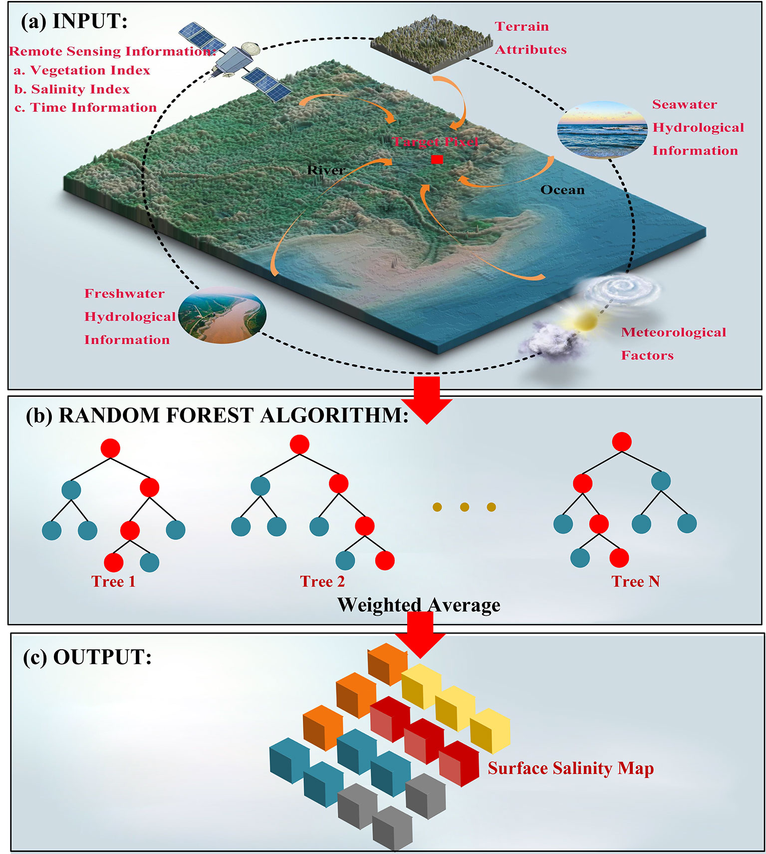
Figure 1 Structure and specific schematics of the random forest model based on hydrological connectivity metric. (A) The model benefited from rich information of multi-resource data (including the remote-sensed spectral data, terrain attributes, meteorological data, temporal information, and hydrological connectivity metric). (B) The constructed random forest model integrated output results of all decision trees based on weighted average mechanism. (C) The model obtained the best estimation of surface soil salinity of each pixel.

The hydrological characteristics of pixel affected by freshwater (D_f) and saltwater (D_s) sources are expressed by the following equations:

$\begin{array}{ll}{D}_f=\underset{\left(x_f,x_f\right)\in R_f}{\min }{\left[{\left(x_0-x_f\right)}^2+{\left(y_0-y_f\right)}^2\right]}^{\frac{1}{2}}& (2)\end{array}$

and

$\begin{array}{ll}{D}_s=\underset{\left(x_s,x_s\right)\in R_s}{\min }{\left[{\left(x_0-x_s\right)}^2+{\left(y_0-y_s\right)}^2\right]}^{\frac{1}{2},}& (3)\end{array}$

where (x₀, y₀), (x_f, y_f) and (x_s, y_s) were the metric latitude and longitude coordinates of the target pixel, freshwater source pixel, and saltwater source pixel, respectively; R_f and R_s were collections of all fresh and saltwater source pixel metric coordinates separately.

Predictions with low accuracy may result from a single model which attempts to consider all factors driving soil salinity in different types of coastal wetlands. Thus, the study area was divided into NR (dominated by natural factors) and IAA (dominated by anthropogenic factors) according to the land use coverage map in Figure 2C. Two sub-models were developed by applying the random forest algorithm to NR and IAA separately.

FIGURE 2

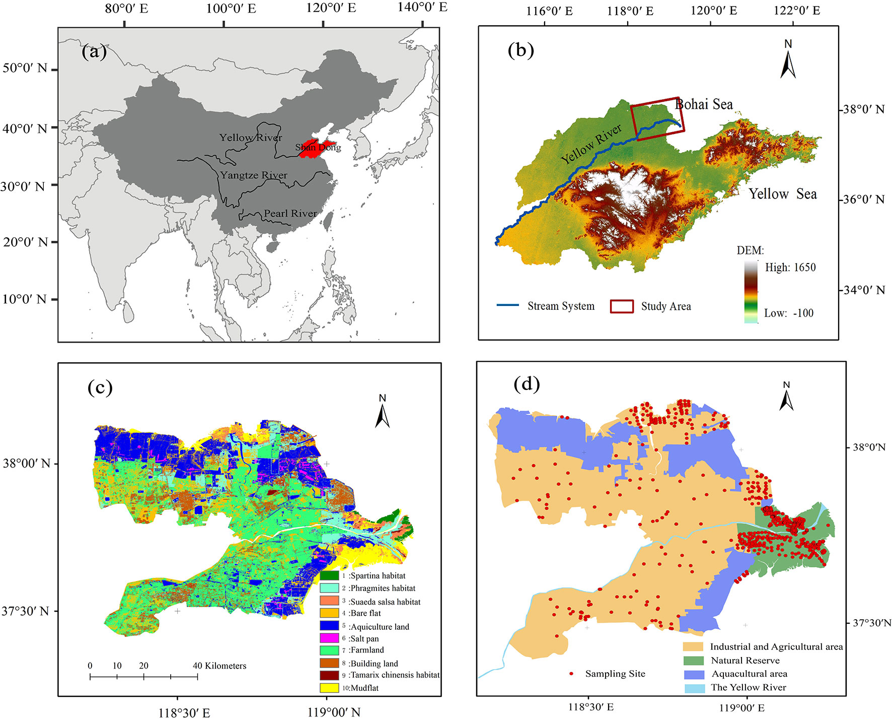
Figure 2 Location of the Yellow River delta, China. (A) Map of China, (B) digital elevation map of Shandong, (C) land use cover types for 2016 from the Landsat 8 OLI image at 30-m spatial resolution, and (D) sampling points (red dots) in the Yellow River delta.

For NR:

$$\left[\text{SAL=f}\left(\text{WIN},\text{SSD},\text{NDVI},\text{PC}2,\text{S}1,\text{S}4,{\text{TC}}_{\text{fou}},\text{CNBL},\text{CD},\text{CI},\text{TWI},\text{VD},{\mathrm{D}}_{\text{f}},{\mathrm{D}}_{\text{s}},{\mathrm{D}}_{\text{t}}\right)\right]$$

For IAA:

$$\left[\text{SAL=f}\left(\text{PC}1,\text{S}2,\text{S}4,\text{SI}1,{\text{TC}}_{\text{bri}},{\text{TC}}_{\text{fif}},\text{CNBL},{\mathrm{D}}_{\text{f}},{\mathrm{D}}_{\text{s}},{\mathrm{D}}_{\text{t}}\right)\right]$$

Based on Python programming language, the two sub-models were each trained by splitting the dataset into two subsets on the basis of random sampling. Each subset is divided into 10 parts, nine of which were rotated to train and build the model, and one was used to validate the performance of the model. Finally, a dataset comprised of the prepared input variables was utilized to the trained model. The output was surface soil salinity estimation over a 30 × 30-m grid at 0–10-cm depths. The methodology flow chart of the models is shown in Figure 3.

FIGURE 3

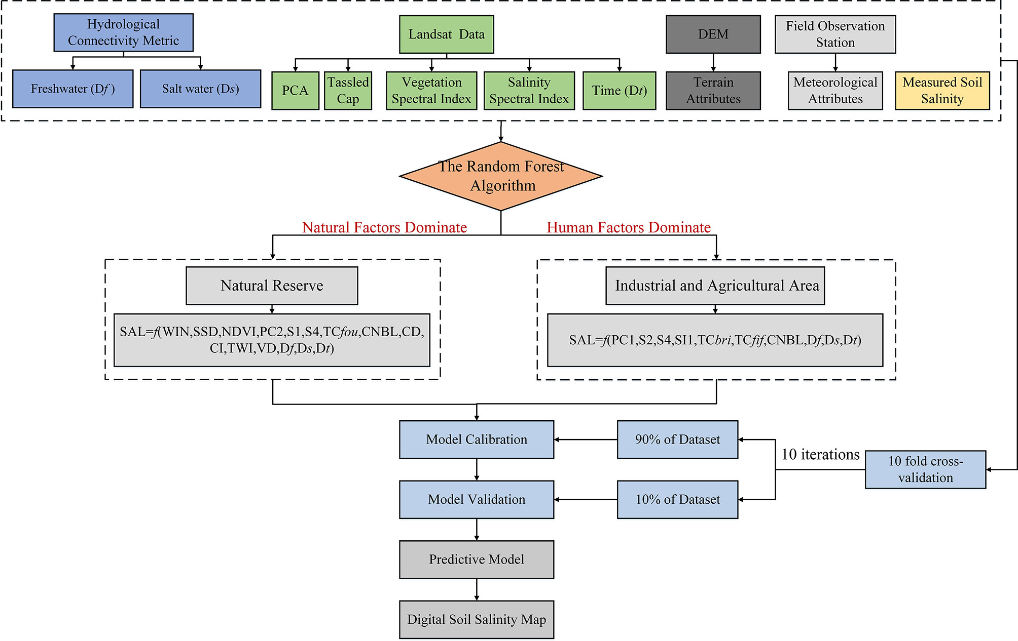
Figure 3 Flow chart of the methodology used for soil salinity estimation in this study.

3.2.2 Permutation Importance and Variable Selection

The random forest model provides the permutation importance measures for all predictor variables and an estimation of the importance of each predictor variable and can determine the mean difference between the predictor accuracy of each tree (Hu et al., 2017) before and after the random permutation of predictor variables. Higher estimated importance values indicate stronger correlations between predictor variables and response variables (Strobl et al., 2008). In this study, the random forest model provided two types of variable importance measure methods [the increase in MSE and node purities (hereafter referred to as Inc.MSE and Inc.NP, respectively) (Hu et al., 2017)] in the training process to improve the prediction accuracy. Since not all satisfied variables of condition can be used to predict the output variable, some unrelated variables may reduce the accuracy of the model. Thus, the variable selection was significant to eliminate the unrelated variables to improve the accuracy of the model and avoid overfitting. In general, models with less variables tend to be more interpretable; thus, a grid research method was used in this study on Linux server (Batten et al., 2019). First, based on the default parameter values, the best variable combination is identified by comparing the 10-fold cross-validation results of the models (i.e., the RF, MLR, PLSR, and GWR models) with different variable combinations (for the best variable combinations of the four models, see Supplementary Table S8 for details). Then, we determine the best parameter combinations using the same approaches based on the best variable combination.

3.3 Contrast Models

The MLR model is a traditional parameter regression model, expressed as detailed below:

For NR:

$\begin{array}{ll}SA{L}_1=a_{1}WIN+a_{2}PRE+a_{3}RHU\dots +a_n{D}_t+\text{b,}& (4)\end{array}$

For IAA:

$\begin{array}{ll}SA{L}_2=a_1\text{SSD+}{a}_{2}S2+a_{3}S4+\dots a_n{D}_s+\text{b,}& (5)\end{array}$

where a₁, …, a_n are the regression coefficients, and b is the intercept.

The GWR model allows a parameter estimated from a linear regression model to vary locally (Yu et al., 2020). This can reduce the change in relationship of variables due to geographical location change.

The GWR model is expressed as detailed below:

For NR:

$\begin{array}{ll}SA{L}_{1l}=b_0\left(\text{i,j}\right)+b_1\left(i,j\right)\text{WIN+}{b}_2\left(i,j\right)\text{PRE+}{b}_3\left(i,j\right)\text{SSD}+\dots +b_n\left(i,j\right)D_t+{\epsilon }_l,& (6)\end{array}$

For IAA:

$\begin{array}{ll}SA{L}_{2l}=b_0\left(i,j\right)+b_1\left(i,j\right)+\text{SSD+}{b}_2\left(i,j\right)\text{PC}1+b_3\left(i,j\right)+\text{SI}1+\dots b_n\left(i,j\right)D_t+{\epsilon }_l,& (7)\end{array}$

where SAL₁ is the soil salinity at location l (i, j), b₀ is the intercept, b₁–b_n are the slopes for each independent variable, and ϵ is for the error term.

The PLSR model is the most commonly used method of building a multi-independent model that can handle data with strong collinearity and noise and has been widely used in satellite remote sensing monitoring of soil salinization (Fan et al., 2015; Peng et al., 2019), expressed as detailed below:

For NR:

$\begin{array}{ll}\left[{SAL}_{1p}=f\left(\text{WIN},\text{PRE},\text{RHU},\text{SSD},\text{PC}2,\text{PC}3,\text{S}5,T{C}_{fif},T{C}_{fou},\text{CNBL},\text{CI},\text{CSC},\text{VD},D_s,D_t\right)\right]& (8)\end{array}$

For IAA:

$\begin{array}{ll}\left[{SAL}_{2p}=f\left(\text{SSD},\text{S}2,T{C}_{bri},\text{CNBL},\text{GEO},D_s\right)\right]& (9)\end{array}$

3.4 Model Performance Evaluation

In this study, the 10-fold cross-validation approach is selected to validate soil salinity estimated by the proposed RF model, MLR model, GWR model, and PLSR model. Moreover, we use four indexes, i.e., the coefficient of determination (R²), the root mean square error (RMSE), the mean absolute error (MAE), and the ratio of performance to deviation (RPD), to evaluate the performance of the above-mentioned models. A well-performed model will have higher R² and RPD values, with lower RMSE and MAE. Additionally, Pearson’s correlation coefficient is used to evaluate the sensitivity of the models to hydrological changes. A model that is sensitive to hydrological changes will have a high Pearson’s correlation coefficient.

4 Results

4.1 Descriptive Statistics

The results of bivariate correlation analysis (Supplementary Tables S4, S5) show that all the independent variables used to fit both models are significantly related to soil salinity, especially CNBL (r = 0.27, p<0.01), D_f (r = 0.21, p < 0.01), and D_s (r = -0.20, p < 0.01) in the NR and TC_fif (r = -0.18, p < 0.01) and D_f (r = 0.2, p < 0.01) in the IAA. Additionally, the multi-collinearity analysis for variables in both models indicates that, in all cases, the extent of collinearity is relatively low, with the highest VIF of variables in NR and IAA sub-models at 11.62 and 5.63, respectively (Supplementary Tables S6, S7).

The overall descriptive statistics of the final variable datasets for the NR and IAA sub-models are shown in Supplementary Tables S9, S10. There is significant difference in the statistics of soil salinity datasets between NR and IAA, and the soil salinity of both areas show a high spatial variation with variation coefficients (VC) of 0.99 and 0.81. Moreover, many variables also show a high spatial variation in more than 50% of the VC, including D_f, D_s,TC_fou, NDVI, CD, and CI variables in the NR sub-model and D_f, D_s, and S2 in the IAA sub-model (Supplementary Tables S9, S10).

Furthermore, a significant seasonal variation occurs in several of the variables used to fit both models. The average soil salinity in the NR exhibits large seasonal variations (5.22 g·kg^–1 in spring, 5.22 g·kg^–1 in summer, 5.89 g·kg^–1 in autumn, and 3.40 g·kg^–1 in winter). The NDVI also varies with the seasons, with the highest value of 0.16 in winter and the lowest value of 0.12 in autumn. In the IAA, the highest average soil salinity occurs in winter (9.91 g·kg^–1) and the lowest (4.94 g·kg^–1) in autumn. The seasonal statistics for all selected variables for both models are shown in Supplementary Tables S11 and S12.

4.2 Model Fitting and Validation

Figure 4 shows the scatterplots of the fitting results for the proposed RF model and for currently popular regression models, including the MLR, GWR, and PLSR models. The same datasets of NR and IAA are used in all models. In the NR, the proposed RF model performs relatively well at model-fitting results (R² = 0.97, RMSE = 0.75 g·kg^–1, and MAE = 0.54 g·kg^–1). The statistical results for the MLR, GWR, and PLSR models are relatively worse, with lower R² and higher RMSE and MAE. In the IAA, the proposed RF model also gives a better fitting result, with higher R² (0.94), lower RMSE (1.24 g·kg^–1), and lower MAE (0.87 g·kg^–1). The fitting results for the MLR, GWR, and PLSR models are worse, all with R² <0.75. In conclusion, the random forest algorithm can give a better performance at training approximations in bulk data with high-dimensional features rather than the parametric (MLR) model and the non-parametric models (GWR and PLSR).

FIGURE 4

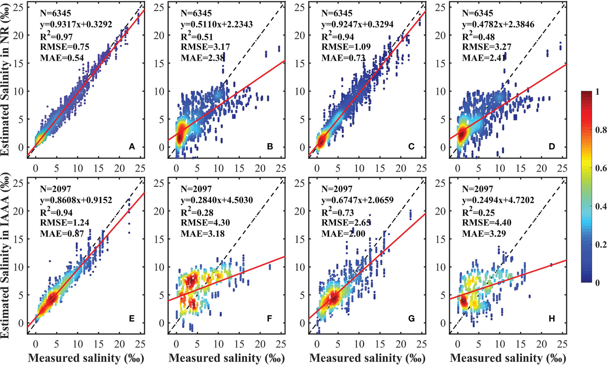
Figure 4 Scatterplots of the model fitting results of the random forest model (A, E), the multiple linear regression model (B, F), the geographically weighted regression model (C, G), and the partial least squares regression model (D, H). The color represents the density of the point. The black dashed and red solid lines represent the 1:1 line and the linear regression line, respectively.

The validation results for the proposed RF model and for the MLR, GWR, and PLSR models are shown in Figure 5. In the NR, the validation results of the MLR, GWR, and PLSR models are bad (R² = 0.49, 0.78, and 0.46 respectively), whereas the proposed RF model shows a better performance, with R² = 0.89, RMSE = 1.48 g·kg^–1, MAE = 1.05 g·kg^–1, and RPD = 3.06. Compared with the other three models, the proposed RF model improves the accuracy by about 11–43%. In the IAA, the proposed RF model also has good performance, with R² = 0.67, RMSE = 2.76 g·kg^–1, MAE = 2.07 g·kg^–1, and RPD = 1.87. The validation results of the MLR, GWR, and PLSR models are also worse than the proposed RF model, with R² = 0.27, 052, and 0.25, respectively. Additionally, the predictions of the RF, MLR, GWR, and PLSR models are less accurate than for NR by 22, 22, 26, and 21%, respectively. The fitted curves show that all four models have the tendency to underestimate the salinity, for all the curve slopes are <1, while the proposed RF model has the highest slope values (0.86 in NR and 0.67 in IAA). The comparison illustrates that the proposed RF model has sufficient accuracy in modeling and estimating soil salinity due to its ability to consider both temporal and hydrological connectivity.

FIGURE 5

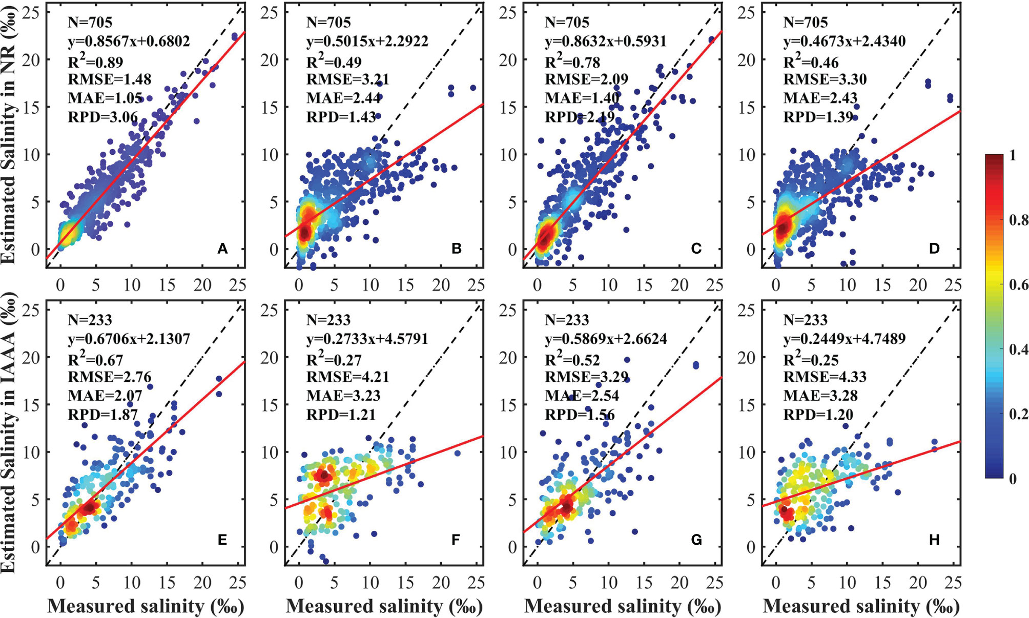
Figure 5 Scatterplots of the model cross-validation results of the random forest model (A, E), the multiple linear regression model (B, F), the geographically weighted regression model (C, G), and the partial least squares regression model (D, H). The color represents the density of the point. The black dashed and solid lines represent the 1:1 line and the linear regression line, respectively.

4.3 Model Performance Comparison Among Seasons

The seasonal performance of the proposed RF, MLR, GWR, and PLSR models, respectively, are compared in this section based on NR and IAA datasets (Table 1). In spring, the proposed RF model in NR has the best performance among the five models, with the highest R² of 0.83, the lowest RMSE of 1.53 g·kg^–1, and the lowest MAE of 1.09 g·kg^–1. In this season, the MLR and PLSR models give worse validation results with R² = 0.72 and 0.46, respectively. The GWR model is the least accurate of the five models (R² = 0.07, RMSE = 15.28 g·kg^–1, and MAE = 7.28 g·kg^–1). In the IAA, the proposed RF model performs well, with R² = 0.42, RMSE = 3.35 g·kg^–1, and MAE = 2.58 g·kg^–1. The performances of the other three models are inferior, with R² <0.

TABLE 1

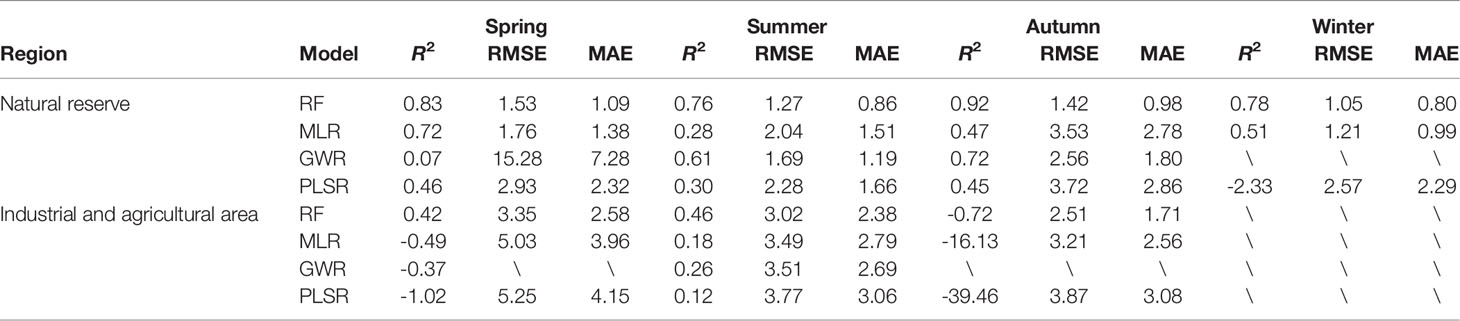
Table 1 Statistics for the comparison of seasonal model cross-validation performance.

For the summer season in both of NR and IAA, the proposed RF model produces the best results of the five (for NR, R² = 0.76, RMSE = 1.27 g·kg^–1, and MAE = 0.86 g·kg^–1; for IAA, R² = 0.46, RMSE = 3.02 g·kg^–1, and MAE = 2.38 g·kg^–1). The MLR, GWR, and PLSR models give less acceptable validation results [for NR, R² (MLR) = 0.28, R² (GWR) = 0.61, and R² (PLSR) = 0.30; for IAA, R² (MLR) = 0.18, R² (GWR) = 0.26, and R² (PLSR) = 0.12].

For the autumn season, in the NR, the validation accuracy of MLR, GWR, and PLSR gave a poor performance (R² = 0.47, 0.72, and 0.45, respectively). In comparison, the proposed RF model performance is better (R² = 0.92, RMSE = 1.42 g·kg^–1, and MAE = 0.98 g·kg^–1). In the IAA, the proposed RF model and the MLR and PLSR models all perform poorly, with R² <0. In addition, due to the distribution of sampling sites and the scarcity of observational data, the GWR model cannot be constructed in the IAA.

In winter, the performance of the proposed sub-model is the best of the four models in the NR (R² = 0.78, RMSE = 1.05 g·kg^–1, and MAE = 0.80 g·kg^–1). The validation results of the MLR and PLSR models (R² = 0.51 and -2.33, respectively) are both worse than for the proposed RF model. Moreover, the observational data in winter for both areas cannot be used again to build the GWR model in the NR and the four models used in IAA.

The predictions of the proposed RF model overall are more accurate than for the other three models in each season, except for autumn and winter in the IAA. Especially in the NR, the soil salinity prediction accuracy of the proposed RF model is improved by 11, 15, 20, and 27% at least in spring, summer, autumn, and winter, respectively.

4.4 Spatiotemporal Distribution of Estimated Salinity

4.4.1 Spatial Distribution of Estimated Salinity

Figure 6 shows that the proposed RF model can provide a complete 30-m grid spatial coverage of soil salinity, except in water-covered areas (i.e., aquaculture areas and rivers). The spatial distributions of the estimated mean salinity using the proposed RF model at different seasons from 2006 to 2018 in the NR and IAA of YRD is highly heterogeneous spatially and varies with time. In the NR, the annual mean salinity from 2006 to 2018 is 5.75 ± 1.73 g·kg^–1. Areas with the lowest salinity values (<4 g·kg^–1) are mainly near a freshwater body, such as the river channel and the freshwater restoration areas (Figure 6A). However, the soil salinity in the southern and northwestern NR, in which tidal creeks are densely distributed, is generally high (>8 g·kg^–1; Figure 6A). Moreover, regions of high (>8 g·kg^–1) and low (<4 g·kg^–1) salinity have more areas in warm seasons (Figure 6B) than in cold seasons (November – April; Figure 6C). This might suggest the seasonal variation of soil salinity in the NR.

FIGURE 6

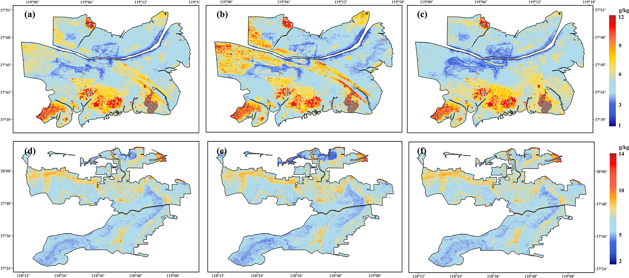
Figure 6 Spatial distribution of the estimated mean salinity from 2006 to 2018 in (A) the nature reserves (NR) all year round, (B) the NR in warm seasons (from May to October), (C) the NR in cold seasons (from November to April), (D) the industrial and agricultural areas (IAA) all year round, (E) the IAA in warm seasons (from May to October), and (F) the IAA in cold seasons (from November to April).

In the IAA, the annual mean salinity from 2006 to 2018 is higher than in the NR, with a value of 6.52 ± 1.07 g·kg^–1. The regions with high soil salinity (>8 g·kg^–1; Figure 6D) are mainly found near a saltwater body, mainly the coastline. It was also found that some urban areas have relatively higher soil salinity, whereas the salinity near the river channel is generally low (<4 g·kg^–1; Figure 6D). Generally, the soil salinity distribution in the IAA varies less between warm and cold seasons (Figures 6E, F).

4.4.2 Monthly Variation of Estimated Salinity

The monthly mean salinity of YRD fluctuates with time in different regions (Figure 7). For the overall study area, the maximum and minimum soil salinity values appear in January (mean = 7.56 g·kg^–1, σ = 3.09) and April (mean = 5.13 g·kg^–1, σ = 1.95). The monthly variation in the NR also shows a similar trend, but with more fluctuation. The maximum and minimum salinity values appear in December (mean = 7.14 g·kg^–1, σ = 2.14) and April (mean = 3.53 g·kg^–1, σ = 1.76). The monthly mean soil salinity in the IAA varies only slightly compared with NR and the overall YRD, with mean salinity range of less than ± 1.15 g·kg^–1 in different months.

FIGURE 7

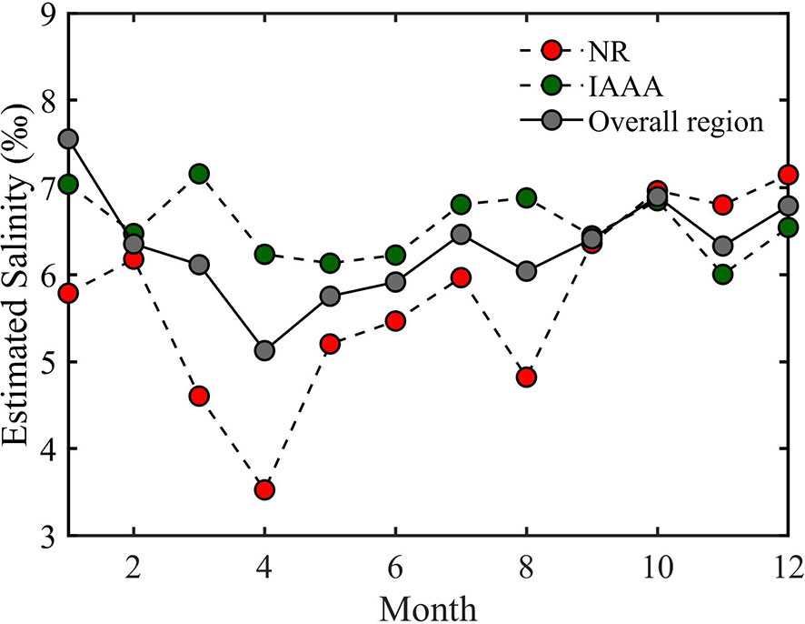
Figure 7 Monthly mean variation of the estimated salinity from 2006 to 2018 in the nature reserves, the industrial and agricultural areas, and the overall Yellow River Delta.

4.5 Hydrological Sensitivity of the Proposed RF Model

The results of the variable importance evaluation for predicting variables in the proposed RF models of the NR and IAA are shown in Figure 8. Two indicators are used to evaluate the sensitivity of the proposed RF model: the increase in mean square errors (Inc.MSE) and the increase in node purities (Inc.NP). The permutation from both evaluation indicators revealed that, in NR, D_t and D_f are two of the most sensitive variables (Figures 8A, C). This might illustrate that the spatial distribution of freshwater and the time variation are both the key factors affecting the soil salinity distribution in this area. In IAA, the CNBL variable is the most important predictor variable from both evaluation indicators (Figures 8B, D). In contrast to the NR, the soil salinity of this region might be affected more by the topography. D_f is the second most important predictor from both evaluation indicators (Figures 8B, D), which means that the spatial distribution of freshwater is still the key factor to soil salinity distribution, while D_t is ranked lower by both important measures than in NR. Totally speaking, the freshwater hydrological variations are the key factors determining the distribution and variation of the surface soil salinity in the whole Yellow River Delta.

FIGURE 8

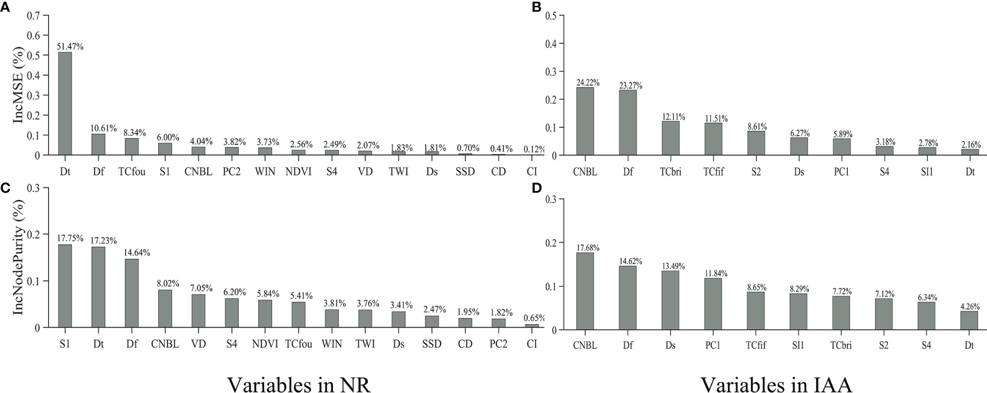
Figure 8 Variable importance permutation of (A) the nature reserves (NR) by Inc.MSE, (B) the industrial and agricultural areas (IAA) by Inc.MSE, (C) the NR by Inc.NP, and (D) the IAA by Inc.NP.

To further examine the sensitivity to hydrological variations of the monthly mean salinity generated by different models, the correlations between the monthly mean salinity generated by the models and the monthly runoff of Yellow River at Lijin station are analyzed. The result shows that the monthly mean salinity of the proposed RF model (r = 0.46, p < 0.01) is significantly correlated with the runoff at Lijin station, while the values of other models have no significant correlation with runoff (MLR model, r = 0.31, p = 0.08; PLSR model, r = –0.03, p = 0.86). This might indicate that the monthly mean salinity values estimated by the proposed RF model are more sensitive to the monthly hydrological variations than by the other models.

5 Discussion

In this study, a combination of random forest algorithm and hydrological connectivity metric is used for the first time in a soil salinity-predicting model. The assessment result (Figures 4, 5) shows that the RF model has a higher prediction accuracy than the other current models (i.e., MLR, GWR, and PLSR models). In comparison with former studies in arid regions or inland salt marshes, the 10-fold cross-validation R² from the proposed RF model is comparable with the traditional validation results of the cubist model (Peng et al., 2019), the bootstrap-BP neural network model (Wang et al., 2018), and the supported vector regression model (Aldabaa et al., 2015). Similar to the proposed RF model, the former models used similar predictor variables, such as vegetation spectral index, salinity spectral index, terrain attributions, and meteorological data (Allbed et al., 2014; Scudiero et al., 2015; Peng et al., 2019).

However, the variables with low importance are not included in the final proposed RF model, such as brightness index, enhanced vegetation index, normalized differential salinity index, elevation, aspect, ground surface temperature, etc. In fact, the inclusion of those variables is found to reduce the prediction accuracy. Other variables, including the time (D_t), minimum distance from freshwater source (D_f), and minimum distance from saltwater source (D_s), have not been used in previous studies. These variables are proven to increase the prediction accuracy in the final model (Figure 8).

The random forest algorithm provides two categories of importance measures for variables during the training process: increase of mean square error and node purities (Hu et al., 2017). Those categories can bring additional insights into the predictor variables and greatest improvements into the prediction accuracy.

In addition, this algorithm can also generate a monthly soil salinity dataset and provide a higher prediction accuracy than the MLR, GWR, and PLSR models among seasons (Table 1). Even though the proposed RF model is optimized for all seasons rather than for each season individually, on the seasonal scale, compared with the other studies, the predictive accuracy of this model based on 10-fold CV is similar with those of the studies conducted by Wang et al. (2018) in spring and Taghizadeh-Mehrjardi et al. (2014) in summer based on traditional validation.

In most previous studies, a regression relationship was established between the observed salinity and the input variables for a single point—for instance, Fan et al. (2015); Peng et al. (2019), and Masoud (2014) utilized the soil sample data, in different time periods, to establish the regression model for predicting salinity distribution. Those models can give relatively accurate predictions at those specific periods, while the predictions often face the problem of overfitting at other periods. To solve this problem, the model we established in this research considers the rationality of the spatial distribution of sample sites and the diversity of sampling seasons. The spatiotemporal information is used as input variable for the proposed RF model, which can improve the spatiotemporal sensitivity of the model and the predicting accuracy among seasons. Moreover, the model established in this research is more sensitive to variation in hydrological conditions, such as the distance to freshwater and saltwater sources.

Our results show that the surface soil salinity values near freshwater sources, including river channels and freshwater restoration areas, are generally low (<4 g·kg^–1, Figures 6A, D). The results are similar with those of the former studies, such that the direct or indirect restoration projects of freshwater resources are effective to the relief of soil salinization (Fan et al., 2011; Yu et al., 2014; Yang et al., 2015; Chi et al., 2019). However, the high salinity values (>8 g·kg^–1) are mainly found near saltwater sources, including the coastline, tidal creeks, and aquaculture areas (Figures 6A, D), which are consistent with former studies. Seawater is the main source of soil salinity in those areas, and some physical processes, such as seawater intrusion, precipitation, evaporation, and plant evapotranspiration, can affect the soil salinization of adjacent regions (Russak et al., 2015; Chi et al., 2019). Those processes affect the salinity by soil capillarity and groundwater level (Fan et al., 2012; Jin et al., 2019).

Additionally, the predicted salinity of the proposed RF model shows a better correlation with runoff at Lijin station than the MLR and PLSR models (Table 1). The hydrological variable (D_f) of the proposed RF models for NR and IAA is also the highest among the three models by both importance measures (Figure 8). This suggests that the soil salinity estimations generated by the proposed RF model is highly sensitive to variation in hydrological conditions, along with the environmental factors (Rossetti and Scotton, 2017). Compared with previous studies (Allbed et al., 2014; Bai et al., 2016; Gorji et al., 2017; Wang et al., 2018), the proposed RF model can more precisely match for delta regions and capture the influence of variation more sensitively in hydrological conditions on soil salinity.

Several certain potential limitations are also found in this research. The spatial resolution is the first limitation of the accuracy prediction of soil salinity. The Landsat data with 30-m spatial resolution used in this study have a moderate difference at the pixel level rather than data from satellites with smaller spatial resolutions. Allbed et al. (2014) assessed the salinity in areas using IKONOS satellite data with 1-m spatial resolution, and Neto et al. (2017) demonstrated that the 1-m airbone ProSpecTIR-VS hyperspectral data could give a more accurate salinity prediction than the 30-m Landsat OLI data. Although the 30-m resolution can provide a longer time series and a considerable reduction in computing time compared with the 1-m resolution, the 1-m resolution data will then further improve the prediction accuracy. This will be the next step to improve the model.

Another limitation of the model is that the systematic studies of the mechanisms of hydrological and hydrodynamic changes in coastal areas are not completed yet. The influence of the hydrological and hydrodynamic changes on soil salinity consists of a series of complex physical processes, involving permeation fluid mechanics, hydromechanics, and capillary action. According to a model simulation of Wang et al. (2007), factors such as temperature, evapotranspiration, hydraulic conductivity, tides, and seawater salinity all affect the formation of salinity distribution of coastal tidal flats. Thus, full understanding of the influencing mechanism of the hydrological and hydrodynamic processes on soil salinity is the key to an accurate prediction. This is also the part of our work that needs to be improved in future studies. Finally, although the proposed RF model can give relatively accurate predictions, there is still evidence that the soil salinity is underestimated in the study area, and the extent will be increased in high-salt areas (e.g., high tidal flats) and at some particular times, such as in January. This may be a potential cause to the salinity prediction error.

6 Conclusions

The estuarine wetlands are located in the interlacing interface of land and sea. They can be affected by the interaction of river runoff and seawater, resulting in a complex modification of hydrological processes and soil salinization processes, thereby leading to the spatial and temporal heterogeneity of soil salinity of coastal wetlands. This has become the biggest challenge to traditional salinity estimation models based on satellite data. In this study, we proposed a model by integrating random forest algorithm and hydrological connectivity metric to predict the soil surface salinity of coastal tidal flats. Several independent spatiotemporal environmental factors are also considered in the model as incorporating variables, including temporal information, remote sensing spectral indices of vegetation and soil, terrain and meteorological attributes, etc. The model performance and response sensitivity to hydrological variations are evaluated using 10-fold cross-validation statistical approaches (R², MAE, RMSE, and RPD) and Pearson’s correlation coefficient. A comprehensive analysis is carried out to compare the accuracy and stability with the commonly used MLR, GWR, and PLSR models.

The model performance assessment result shows that the performance of the proposed RF model in this work exhibits a high and stable accuracy, with R² = 0.89, RMSE = 1.48, and MAE = 1.05. The accuracy of the proposed RF model can be increased by about 11–43% over the former MLR, GWR, and PLSR models. The prediction performance of the proposed RF model among seasons is also better than that of the other models. Moreover, on a monthly scale, the model is more sensitive to the variation of the hydrological conditions than the other models. Detailed spatiotemporal and hydrological information is used in the prediction to increase the predicting accuracy of surface soil salinity under the complex condition of estuarine wetlands. In conclusion, the proposed surface soil salinity estimation based on random forest algorithm is satisfactory for soil salinization studies in estuarine wetlands.

Data Availability Statement

The raw data supporting the conclusions of this article will be made available by the authors without undue reservation.

Author Contributions

The conceptualization of this work was developed by HS, JY, and DC. The resources and funding acquisition for this work were provided by JY. HS carried out the research and wrote the initial draft. HS and JY performed the model training and validation and compared our results with the traditional models. JY assessed the variable importance. BL, WL, BC, JY, and DC helped with the refinement of this manuscript. All authors contributed to the article and approved the submitted version.

Conflict of Interest

JY and BL are employed by China Oilfield Services Limited.

The remaining authors declare that the research was conducted in the absence of any commercial or financial relationships that could be construed as a potential conflict of interest.

Publisher’s Note

All claims expressed in this article are solely those of the authors and do not necessarily represent those of their affiliated organizations, or those of the publisher, the editors and the reviewers. Any product that may be evaluated in this article, or claim that may be made by its manufacturer, is not guaranteed or endorsed by the publisher.

Acknowledgments

This work was supported by the Key Project of the National Natural Science Foundation of China (U2243208 and U1901212) and the National Natural Science Foundation of China (51909005).

Supplementary Material

The Supplementary Material for this article can be found online at: https://www.frontiersin.org/articles/10.3389/fmars.2022.895172/full#supplementary-material

References

Abdelkader F. H. (2011). Digital Soil Mapping at Pilot Sites in the Northwest Coast of Egypt: A Multinomial Logistic Regression Approach. Egypt. J. Remote Sens. Space. Sci. 14, 29–40. doi: 10.1016/j.ejrs.2011.04.001

CrossRef Full Text | Google Scholar

Aldabaa A. A. A., Weindorf D. C., Chakraborty S., Sharma A., Li B. (2015). Combination of Proximal and Remote Sensing Methods for Rapid Soil Salinity Quantification. Geoderma 239, 34–46. doi: 10.1016/j.geoderma.2014.09.011

CrossRef Full Text | Google Scholar

Allbed A., Kumar L., Aldakheel Y. Y. (2014). Assessing Soil Salinity Using Soil Salinity and Vegetation Indices Derived From IKONOS High-Spatial Resolution Imageries: Applications in a Date Palm Dominated Region. Geoderma 230, 1–8. doi: 10.1016/j.geoderma.2014.03.025

CrossRef Full Text | Google Scholar

Bai L., Wang C., Zang S., Zhang Y., Hao Q., Wu Y. (2016). Remote Sensing of Soil Alkalinity and Salinity in the Wuyu'er-Shuangyang River Basin, Northeast China. Remote Sens. 8 (2), 163. doi: 10.3390/rs8020163

CrossRef Full Text | Google Scholar

Barbier E. B., Hacker S. D., Kennedy C., Koch E. W., Stier A. C., Silliman B. R. (2011). The Value of Estuarine and Coastal Ecosystem Services. Ecol. Monogr. 81, 169–193. doi: 10.1890/10-1510.1

CrossRef Full Text | Google Scholar

Batten A. J., Thorpe J., Piegari R. I., Rosland A.-M. (2019). A Resampling Based Grid Search Method to Improve Reliability and Robustness of Mixture-Item Response Theory Models of Multimorbid High-Risk Patients. IEEE J. Biomed. Health Inf. 24, 1780–1787. doi: 10.1109/JBHI.2019.2948734

CrossRef Full Text | Google Scholar

Breiman L. (2001). Random Forests. Mach. Learn. 45, 5–32. doi: 10.1023/A:1010933404324

CrossRef Full Text | Google Scholar

Chi Y., Sun J., Liu W., Wang J., Zhao M. (2019). Mapping Coastal Wetland Soil Salinity in Different Seasons Using an Improved Comprehensive Land Surface Factor System. Ecol. Indic. 107, 105517. doi: 10.1016/j.ecolind.2019.105517

CrossRef Full Text | Google Scholar

Cho K. H., Beon M.-S., Jeong J.-C. (2018). Dynamics of Soil Salinity and Vegetation in a Reclaimed Area in Saemangeum, Republic of Korea. Geoderma 321, 42–51. doi: 10.1016/j.geoderma.2018.01.031

CrossRef Full Text | Google Scholar

Chuantao Q., Dinghua L. (1997). The Calculation Algorithms for Average Wind Direction and Their Comparison. Plat. Meteorol. 16, 94–98. doi: 10.1121/1.3277222

CrossRef Full Text | Google Scholar

Contreras-Cruzado I., Dolores Infante-Izquierdo M., Marquez-Garcia B., Hermoso-Lopez V., Polo A., Nieva F. J. J., et al. (2017). Relationships Between Spatio-Temporal Changes in the Sedimentary Environment and Halophytes Zonation in Salt Marshes. Geoderma 305, 173–187. doi: 10.1016/j.geoderma.2017.05.037

CrossRef Full Text | Google Scholar

Cui B., Cai Y., Xie T., Ning Z., Hua Y. (2016). Ecological Effects of Wetland Hydrological Connectivity: Problems and Prospects. J. Beijing Normal. University Natural Sci. 52, 738–746. doi: 10.16360/j.cnki.jbnuns.2016.06.011

CrossRef Full Text | Google Scholar

Davis E., Wang C., Dow K. (2019). Comparing Sentinel-2 MSI and Landsat 8 OLI in Soil Salinity Detection: A Case Study of Agricultural Lands in Coastal North Carolina. Int. J. Remote Sens. 40, 6134–6153. doi: 10.1080/01431161.2019.1587205

CrossRef Full Text | Google Scholar

Fan X., Liu Y., Tao J., Weng Y. (2015). Soil Salinity Retrieval From Advanced Multi-Spectral Sensor With Partial Least Square Regression. Remote Sens. 7, 488–511. doi: 10.3390/rs70100488

CrossRef Full Text | Google Scholar

Fan X., Pedroli B., Liu G., Liu Q., Liu H., Shu L. (2012). Soil Salinity Development in the Yellow River Delta in Relation to Groundwater Dynamics. Land. Degrad. Dev. 23, 175–189. doi: 10.1002/ldr.1071

CrossRef Full Text | Google Scholar

Fan X., Pedroli B., Liu G., Liu H., Song C., Shu L. (2011). Potential Plant Species Distribution in the Yellow River Delta Under the Influence of Groundwater Level and Soil Salinity. Ecohydrology 4, 744–756. doi: 10.1002/eco.164

CrossRef Full Text | Google Scholar

Fan X., Weng Y., Tao J. (2016). Towards Decadal Soil Salinity Mapping Using Landsat Time Series Data. Int. J. Appl. Earth Observ. Geoinform. 52, 32–41. doi: 10.1016/j.jag.2016.05.009

CrossRef Full Text | Google Scholar

Flowers T. J., Colmer T. D. (2015). Plant Salt Tolerance: Adaptations in Halophytes. Ann. Bot-london. 115, 327–331. doi: 10.1093/aob/mcu267

CrossRef Full Text | Google Scholar

Ge X., Wang J., Ding J., Cao X., Zhang Z., Liu J., et al. (2019). Combining UAV-Based Hyperspectral Imagery and Machine Learning Algorithms for Soil Moisture Content Monitoring. Peerj. 7, e6926. doi: 10.7717/peerj.6926

PubMed Abstract | CrossRef Full Text | Google Scholar

Gorji T., Sertel E., Tanik A. (2017). Monitoring Soil Salinity via Remote Sensing Technology Under Data Scarce Conditions: A Case Study From Turkey. Ecol. Indic. 74, 384–391. doi: 10.1016/j.ecolind.2016.11.043

CrossRef Full Text | Google Scholar

Hastie T., Tibshirani R., Friedman J. (2009). The Elements of Statistical Learning: Data Mining, Inference, and Prediction (New York: Springer Science & Business Media).

Google Scholar

Herbert E. R., Boon P., Burgin A. J., Neubauer S. C., Franklin R. B., Ardon M., et al. (2015). A Global Perspective on Wetland Salinization: Ecological Consequences of a Growing Threat to Freshwater Wetlands. Ecosphere 6(10), 1–43. doi: 10.1890/ES14-00534.1

CrossRef Full Text | Google Scholar

Hong W., Tiyip T., Xia X. I. E., Yahui F. A. N., Fei Z., Sawut M. (2011). Assessment of Soil Salinization Sensitivity for Different Types of Land Use in the Ebinur Lake Region in Xinjiang. Prog. Geograph. 30, 593–599. doi: 10.11820/dlkxjz.2011.05.011

CrossRef Full Text | Google Scholar

Hu X., Belle J. H., Meng X., Wildani A., Waller L. A., Strickland M. J., et al. (2017). Estimating PM2.5 Concentrations in the Conterminous United States Using the Random Forest Approach. Environ. Sci. Technol. 51, 6936–6944. doi: 10.1021/acs.est.7b01210

PubMed Abstract | CrossRef Full Text | Google Scholar

Jin G., Mo Y., Li M., Tang H., Qi Y., Li L., et al. (2019). Desalinization and Salinization: A Review of Major Challenges for Coastal Reservoirs. J. Coast. Res. 35, 664–672. doi: 10.2112/JCOASTRES-D-18-00067.1

CrossRef Full Text | Google Scholar

Lee S., Ji K., An Y., Ro H. (2003). Soil Salinity and Vegetation Distribution at Four Tidal Reclamation Project Areas. Kor. J. Environ. Agric. 22, 79–86. doi: 10.5338/KJEA.2003.22.2.079

CrossRef Full Text | Google Scholar

Liang J., Ding J., Wang J., Wang F. (2019). Quantitative Estimation and Mapping of Soil Salinity in the Ebinur Lake Wetland Based on Vis-NIR Reflectance and Landsat 8 OLI Data. Acta Pedologica. Sin. 56, 320–330. doi: 10.11766/trxb201805070182

CrossRef Full Text | Google Scholar

Mahmoodzadeh D., Karamouz M. (2019). Seawater Intrusion in Heterogeneous Coastal Aquifers Under Flooding Events. J. Hydrol. 568, 1118–1130. doi: 10.1016/j.jhydrol.2018.11.012

CrossRef Full Text | Google Scholar

Ma Z., Melville D. S., Liu J., Chen Y., Yang H., Ren W., et al. (2014). ECOSYSTEMS MANAGEMENT Rethinking China's New Great Wall. Science 346, 912–914. doi: 10.1126/science.1257258

PubMed Abstract | CrossRef Full Text | Google Scholar

Masoud A. A. (2014). Predicting Salt Abundance in Slightly Saline Soils From Landsat ETM+ Imagery Using Spectral Mixture Analysis and Soil Spectrometry. Geoderma 217, 45–46. doi: 10.1126/science.1257258

CrossRef Full Text | Google Scholar

Mentaschi L., Vousdoukas M. I., Pekel J.-F., Voukouvalas E., Feyen L. (2018). Global Long-Term Observations of Coastal Erosion and Accretion. Sci. Rep-UK. 8(1), 1–11. doi: 10.1038/s41598-018-30904-w

CrossRef Full Text | Google Scholar

Metternicht G. I., Zinck J. A. (2003). Remote Sensing of Soil Salinity: Potentials and Constraints. Remote Sens. Environ. 85, 1–20. doi: 10.1016/S0034-4257(02)00188-8

CrossRef Full Text | Google Scholar

Peng J., Biswas A., Jiang Q., Zhao R., Hu J., Hu B., et al. (2019). Estimating Soil Salinity From Remote Sensing and Terrain Data in Southern Xinjiang Province, China. Geoderma 337, 1309–1319. doi: 10.1016/j.geoderma.2018.08.006

CrossRef Full Text | Google Scholar

Peng J., Wang J.-q., Xiang H.-y., Teng H.-f., Liu W.-y., Chi C.-m., et al. (2014). Comparative Study on Hyperspectral Inversion Accuracy of Soil Salt Content and Electrical Conductivity. Spectrosc. Spect. Anal. 34, 510–514. doi: 10.3964/j.issn.1000-0593(2014)02-0510-05

CrossRef Full Text | Google Scholar

Pereira C. S., Lopes I., Abrantes I., Sousa J. P., Chelinho S. (2019). Salinization Effects on Coastal Ecosystems: A Terrestrial Model Ecosystem Approach. Philos. Trans. R. Soc. B. 374, 20180251. doi: 10.1098/rstb.2018.0251

CrossRef Full Text | Google Scholar

Richards L. (1954). Diagnosis and Improvement of Saline and Alkali Soils. Soil Sci. 78, 154. doi: 10.1097/00010694-195408000-00012

CrossRef Full Text | Google Scholar

Rodriguez J. F., Saco P. M., Sandi S., Saintilan N., Riccardi G. (2017). Potential Increase in Coastal Wetland Vulnerability to Sea-Level Rise Suggested by Considering Hydrodynamic Attenuation Effects. Nat. Commun. 8 (1), 1–12. doi: 10.1038/ncomms16094

PubMed Abstract | CrossRef Full Text | Google Scholar

Rocha Neto O. C. d., Teixeira A. d. S., Leão R. A. d. O., Moreira L. C. J., Galvão L. S. (2017). Hyperspectral Remote Sensing for Detecting Soil Salinization Using Prospectir-vs Aerial Imagery and Sensor Simulation. Remote Sens. 9, 42. doi: 10.3390/rs9010042

CrossRef Full Text | Google Scholar

Rossetti V., Scotton M. (2017). Topographical, Soil, and Water Determinants of the Vallevecchia Coastal Dune-Marsh System. Ecol. Eng. 105, 32–41. doi: 10.1016/j.ecoleng.2017.04.046

CrossRef Full Text | Google Scholar

Russak A., Yechieli Y., Herut B., Lazar B., Sivan O. (2015). The Effect of Salinization and Freshening Events in Coastal Aquifers on Nutrient Characteristics as Deduced From Field Data. J. Hydrol. 529, 1293–1301. doi: 10.1016/j.jhydrol.2015.07.022

CrossRef Full Text | Google Scholar

Scudiero E., Skaggs T. H., Corwin D. L. (2015). Regional-Scale Soil Salinity Assessment Using Landsat ETM+ Canopy Reflectance. Remote Sens. Environ. 169, 335–343. doi: 10.1016/j.rse.2015.08.026

CrossRef Full Text | Google Scholar

Strobl C., Boulesteix A.-L., Kneib T., Augustin T., Zeileis A. (2008). Conditional Variable Importance for Random Forests. BMC Bioinf. 9 (1), 1–11. doi: 10.1186/1471-2105-9-307

CrossRef Full Text | Google Scholar

Taghizadeh-Mehrjardi R., Minasny B., Sarmadian F., Malone B. P. (2014). Digital Mapping of Soil Salinity in Ardakan Region, Central Iran. Geoderma 213, 15–28. doi: 10.1016/j.geoderma.2013.07.020

CrossRef Full Text | Google Scholar

Tully K., Gedan K., Epanchin-Niell R., Strong A., Bernhardt E. S., Bendor T., et al. (2019). The Invisible Flood: The Chemistry, Ecology, and Social Implications of Coastal Saltwater Intrusion. Bioscience 69, 368–378. doi: 10.1093/biosci/biz027

CrossRef Full Text | Google Scholar

Vermeulen D., Van Niekerk A. (2017). Machine Learning Performance for Predicting Soil Salinity Using Different Combinations of Geomorphometric Covariates. Geoderma 299, 1–12. doi: 10.1016/j.geoderma.2017.03.013

CrossRef Full Text | Google Scholar

Wang J., Hsieh Y. P., Harwell M. A., Huang W. (2007). Modeling soil salinity distribution along topographic gradients in tidal salt marshes in Atlantic and Gulf coastal regions. Ecol. Model. 201, 429–439. doi: 10.1016/j.ecolmodel.2006.10.013

CrossRef Full Text | Google Scholar

Wang J., Ding J., Yu D., Ma X., Zhang Z., Ge X., et al. (2019). Capability of Sentinel-2 MSI Data for Monitoring and Mapping of Soil Salinity in Dry and Wet Seasons in the Ebinur Lake Region, Xinjiang, China. Geoderma 353, 172–187. doi: 10.1016/j.geoderma.2019.06.040

CrossRef Full Text | Google Scholar

Wang S., Fu B., Piao S., Lu Y., Ciais P., Feng X., et al. (2016). Reduced Sediment Transport in the Yellow River Due to Anthropogenic Changes. Nat. Geosci. 9, 38–41. doi: 10.1038/ngeo2602

CrossRef Full Text | Google Scholar

Wang H., Wu X., Bi N., Li S., Yuan P., Wang A., et al. (2017). Impacts of the Dam-Orientated Water-Sediment Regulation Scheme on the Lower Reaches and Delta of the Yellow River (Huanghe): A Review. Global Planet. Change 157, 93–113. doi: 10.1016/j.gloplacha.2017.08.005

CrossRef Full Text | Google Scholar

Wang X., Zhang F., Ding J., Kung H., Latif A., Johnson V. C. (2018). Estimation of Soil Salt Content (SSC) in the Ebinur Lake Wetland National Nature Reserve (ELWNNR), Northwest China, Based on a Bootstrap-BP Neural Network Model and Optimal Spectral Indices. Sci. Tot. Environ. 615, 918–930. doi: 10.1016/j.scitotenv.2017.10.025

CrossRef Full Text | Google Scholar

Wei Y., Shi Z., Biswas A., Yang S., Ding J., Wang F. (2020). Updated Information on Soil Salinity in a Typical Oasis Agroecosystem and Desert-Oasis Ecotone: Case Study Conducted Along the Tarim River, China. Sci. Tot. Environ. 716, 135387. doi: 10.1016/j.scitotenv.2019.135387

CrossRef Full Text | Google Scholar

Wei W., Tang Z., Dai Z., Lin Y., Ge Z., Gao J. (2015). Variations in Tidal Flats of the Changjiang (Yangtze) Estuary During 1950s-2010s: Future Crisis and Policy Implication. Ocean. Coast. Manage. 108, 89–96. doi: 10.1016/j.ocecoaman.2014.05.018

CrossRef Full Text | Google Scholar

Wilson B. J., Servais S., Charles S. P., Mazzei V., Gaiser E. E., Kominoski J. S., et al. (2019). Phosphorus Alleviation of Salinity Stress: Effects of Saltwater Intrusion on an Everglades Freshwater Peat Marsh. Ecology 100 (5), e02672. doi: 10.1002/ecy.2672

PubMed Abstract | CrossRef Full Text | Google Scholar

Wu C., Liu G., Huang C. (2017). Prediction of Soil Salinity in the Yellow River Delta Using Geographically Weighted Regression. Arch. Agron. Soil Sci. 63, 928–941. doi: 10.1080/03650340.2016.1249475

CrossRef Full Text | Google Scholar

Wu C., Liu G., Huang C., Liu Q. (2019). Soil Quality Assessment in Yellow River Delta: Establishing a Minimum Data Set and Fuzzy Logic Model. Geoderma 334, 82–89. doi: 10.1016/j.geoderma.2018.07.045

CrossRef Full Text | Google Scholar

Xu H. (2006). Modification of Normalised Difference Water Index (NDWI) to Enhance Open Water Features in Remotely Sensed Imagery. Int. J. Remote Sens. 27, 3025–3033. doi: 10.1080/01431160600589179

CrossRef Full Text | Google Scholar

Yang L., Huang C., Liu G., Liu J., Zhu A. (2015). Mapping Soil Salinity Using a Similarity-Based Prediction Approach: A Case Study in Huanghe River Delta, China. Chin. Geograph. Sci. 25, 283–294. doi: 10.1007/s11769-015-0740-7

CrossRef Full Text | Google Scholar

Yang S.-H., Liu F., Song X.-D., Lu Y.-Y., Li D.-C., Zhao Y.-G., et al. (2019). Mapping Topsoil Electrical Conductivity by a Mixed Geographically Weighted Regression Kriging: A Case Study in the Heihe River Basin, Northwest China. Ecol. Indic. 102, 252–264. doi: 10.1016/j.ecolind.2019.02.038

CrossRef Full Text | Google Scholar

Yao R., Yang J., Zhang T., Hong L., Wang M., Yu S., et al. (2014). Studies on Soil Water and Salt Balances and Scenarios Simulation Using Saltmod in a Coastal Reclaimed Farming Area of Eastern China. Agr. Water Manage. 131, 115–123. doi: 10.1016/j.agwat.2013.09.014

CrossRef Full Text | Google Scholar

Yu H., Fotheringham A. S., Li Z., Oshan T., Wolf L. J. (2020). On the Measurement of Bias in Geographically Weighted Regression Models. Spat. Stat 38, 100453. doi: 10.1016/j.spasta.2020.100453

CrossRef Full Text | Google Scholar

Yu J., Li Y., Han G., Zhou D., Fu Y., Guan B., et al. (2014). The Spatial Distribution Characteristics of Soil Salinity in Coastal Zone of the Yellow River Delta. Environ. Earth Sci. 72, 589–599. doi: 10.1007/s12665-013-2980-0

CrossRef Full Text | Google Scholar

Yu H., Wang L., Wang Z., Ren C., Zhang B. (2019). Using Landsat OLI and Random Forest to Assess Grassland Degradation With Aboveground Net Primary Production and Electrical Conductivity Data. Isprs. Int. J. Geo-Informat. 8 (11), 511. doi: 10.3390/ijgi8110511

CrossRef Full Text | Google Scholar

Zhou H., Li W. (2013). The Effects of Oasis Ecosystem Hydrological Processes on Soil Salinization in the Lower Reaches of the Tarim River, China. Ecohydrology 6, 1009–1020. doi: 10.1002/eco.1415

CrossRef Full Text | Google Scholar