 Ronald B. Souza1*
 Margareth S. Copertino2,3
 Gilberto Fisch4
 Marcelo F. Santini5
 Walter H. D. Pinaya6
 Fabiane M. Furlan7
 Rita de Cássia M. Alves7
 Osmar O. Möller Jr.2
 Luciano P. Pezzi5
- 1Earth System Numerical Modeling Division, National Institute for Space Research (INPE), Cachoeira Paulista, Brazil
- 2Institute of Oceanography, Federal University of Rio Grande (FURG), Rio Grande, Brazil
- 3Brazilian Network on Global Climate Change Research (Rede CLIMA), National Institute for Space Research (INPE), São José dos Campos, Brazil
- 4Agricultural Science Department, University of Taubaté (UNITAU), Taubaté, Brazil
- 5Earth Observation and Geoinformatics Division, National Institute for Space Research (INPE), São José dos Campos, Brazil
- 6Secretariat of Aquaculture and Fisheries, Ministry of Agriculture, Livestock and Food Supply, Brasília, Brazil
- 7State Center for Remote Sensing and Meteorology Research, Federal University of Rio Grande do Sul (CEPSRM/UFRGS), Porto Alegre, Brazil
Blue carbon ecosystems are recognized as carbon sinks and therefore for their potential for climate mitigation. While carbon stocks and burial rates have been quantified and estimated regionally and globally, there are still many knowledge gaps on carbon fluxes exchanged particularly at the interface vegetation-atmosphere. In this study we measured the atmospheric CO2 concentrations in a salt marsh located in the Patos Lagoon Estuary, southern Brazil. Eddy correlation techniques were applied to account for the CO2 exchange fluxes between the vegetation and the atmosphere. Our dataset refers to two sampling periods spanning from July up to November 2016 and from January to April 2017. By using time series analysis techniques including wavelet and cross-wavelet analysis, our results show the natural cycles of the CO2 exchanges variability and the relationship of these cycles with other environmental variables. We also present the amplitudes of the salt marsh-atmosphere CO2 fluxes’ diurnal cycle for both study periods and demonstrate that the CO2 fluxes are modulated by the passage of transient atmospheric systems and by the level variation of surrounding waters. During daytime, our site was as a CO2 sink. Fluxes were measured as -6.71 ± 5.55 μmol m-2 s-1 and -7.95 ± 6.44 μmol m-2 s-1 for the winter-spring and summer-fall periods, respectively. During nighttime, the CO2 fluxes were reversed and our site behaved as a CO2 source. Beside the seasonal changes in sunlight and air temperature, differences between the two periods were marked by the level of marsh inundation, winds and plant biomass (higher in summer). The net CO2 balance showed the predominance of the photosynthetic activity over community respiration, indicating the role of the salt marsh as a CO2 sink. When considering the yearly-averaged net fluxes integrated to the whole area of the Patos Lagoon Estuary marshes, the total CO2 sink was estimated as -87.6 Mg C yr-1. This paper is the first to measure and study the vegetation-atmosphere CO2 fluxes of a salt marsh environment of Brazil. The results will contribute to the knowledge on the global carbon budget and for marsh conservation and management plans, including climate change policies.
Introduction
Salt marshes are among the most biologically productive ecosystems in the world, providing a range of valuable ecosystem services to coastal communities (Adam, 1993; Himes-Cornell et al., 2018). Being sources and sinks of nutrients and organic matter to estuaries, salt marshes regulate local biogeochemical cycles, immobilize pollutants and provide habitat for wildlife. Positioned at the intertidal zone at the interface between land and ocean, salt marshes reduce the energy of waves and currents, bind the sediments, provide flood defense and shoreline erosion control, therefore protecting the coast against sea level rise. With high rates of primary production, plant biomass growth and sediment vertical accretion, salt marshes are highly efficient in organic carbon sequestration and storage, together with mangrove forest and seagrass meadows (Duarte et al., 2005; McLeod et al., 2011; Macreadie et al., 2012). Compared to mangrove and seagrass ecosystems, salt marshes have the highest capacity for carbon sequestration, showing accumulation rates up to 244.7 ± 26.1 g C m-2 yr-1 (Chmura et al., 2003; Ouyang and Lee, 2014) and storing an average of 130 Mg C ha-1 (Howe et al., 2009), mostly in the soil and roots and detritus. Despite of their low areal cover relative to the ocean and other terrestrial ecosystems (0.1 – 2%), total carbon accumulation rates in global salt marsh soil are estimated at ~10.2 Tg C yr−1 (Ouyang and Lee, 2014). While the global storage capacity of coastal wetlands is lower compared to the size of terrestrial carbon sinks, the carbon sequestration capacity by salt marsh sediments per unit area is ranked highest amongst coastal wetland and forested terrestrial ecosystems. Furthermore, salt marshes can immobilize the organic carbon for centuries or millennia, whereas terrestrial forests usually only store organic carbon for decades (Macreadie et al., 2012). Therefore, salt marshes are well recognized as blue carbon ecosystems with potential to contribute to regulation of atmospheric CO2 concentrations and mitigate climate change (MacLeod et al., 2011).
Despite their importance in providing ecosystem services, salt marshes have been destroyed for centuries (Duarte et al., 2013). Between 2 and 60% of salt marshes have been lost from the temperate regions of the Earth during last 50 years, particularly due to landscape conversion for housing and farming (Lokwood and Drakeford, 2021). Once the marsh soil is disturbed, the oxidized organic matter is decomposed and large amounts of ancient buried C can be released into the atmosphere as CO2, therefore contributing to greenhouse gases (GHG) emissions (Pendleton et al., 2012; Lovelock et al., 2017). Therefore, both conservation and restoration of salt marshes can maintain carbon sinks and avoid further emissions.
Both salt marshes and mangroves are recognized by the International Panel on Climate Change (IPCC) as potential nature-based solutions for atmospheric CO2 reduction (IPCC, 2021) and therefore eligible to be included within national greenhouse gas accounting frameworks (IPCC, 2014). Additionally, efforts are emerging to use salt marsh conservation and restoration in carbon offset programs, like the “Reducing Emissions from Deforestation and Forest Degradation in Developing Countries (REDD)” initiative for tropical forests (Gibbs et al., 2007). However, the mitigation capacity of a blue carbon ecosystem is a balance between the CO2 sequestrated and emitted (Taillard et al., 2018) and those processes are affected by spatial and temporal variability in natural and anthropogenic disturbances.
While blue carbon science has advanced at unprecedent rates over the last decade, some aspects are still controversial (Lovelock and Duarte, 2019). Among the emerging questions are ones related to the net flux of CO2 and other greenhouse gases between the vegetation/soil/water system and the atmosphere (Macreadie et al., 2019). Even though those ecosystems are significant carbon reservoirs, they can be temporally net emitters of CO2 to atmosphere, depending on the natural dynamics of organic and inorganic carbon exchange. There is a lack of empirical evidence of CO2 fluxes and the processes controlling the exchanges of carbon between the vegetation/soil/water system and overlying atmosphere at the ecosystem level (e.g. Goulden et al., 2007) and how the CO2 fluxes can be influenced by tidal cycles, hydrology, weather, and climate conditions (Polsenaere et al., 2012). Furthermore, anthropogenic disturbances can shift the system from carbon source to sinks (Pendleton et al., 2012; Lovelock et al., 2017). Thus, accurate global blue carbon budgets are limited by uncertainties in CO2 net fluxes.
Micrometeorological flux methods like the eddy covariance (EC) techniques allow the study of whole ecosystem fluxes of CO2 to estimate gross primary production, net ecosystem exchange, and ecosystem respiration (Forbrich and Giblin, 2015). The balance between CO2 released and taken up by the ecosystem is measured, without disturbing the soil or vegetation, and modeling approaches allow the partitioning into the component fluxes of primary production and respiration. Developed initially for terrestrial ecosystems, the EC technique is not yet widely applied in coastal wetland studies, where tidal and hydrological dynamics offer challenges (e.g. Barr et al., 2010; Forbrich and Giblin, 2015; Chu et al., 2021; Hawman et al., 2021; Hill et al., 2021). The knowledge gaps of CO2 fluxes are particularly large for South America, where the great majority of EC studies are concentrated in the terrestrial ecosystems, with few studies performed in coastal wetlands (e.g. Tonti et al., 2018, Freire et al., 2022) and the coastal and open ocean (Pezzi et al., 2016; Oliveira et al., 2019; Santini et al., 2020; Pezzi et al., 2021; Souza et al., 2021).
In the Southwestern Atlantic Ocean, southern South America, salt marshes dominate the intertidal estuarine habitats of the subtropical and temperate coastline covering approximately 5,000 km of coastline from 29° S to 54° S with an area of approximately 220,000 ha (Isacch et al., 2006; Martinetto et al., 2016). Extensive coastal wetlands are found surrounding the Patos Lagoon Estuary (Costa et al., 2003), a dominant feature of the southern Brazil coastal plain that is of high ecological and social relevance (Odebrecht et al., 2010; Odebrecht et al., 2017). Well preserved and highly productive salt marshes occupy about 70 km2 of the margins of Patos Lagoon Estuary (Nogueira and Costa, 2003; Costa and Marangoni, 2010). The Patos Lagoon salt marshes are strongly affected by seasonal changes of light, temperature and hydrological cycles (Costa, 1997a; Costa, 1997b; Costa e Marangoni, 2010). Preliminary results show these salt marshes store an average of 220 Mg C ha-1 (Paterson, 2016), which is in the high range of the global observations. A large area of the Patos Lagoon salt marshes has been lost and degraded since the early nineteenth century by urbanization, agriculture activities, industrial and port expansion (Costa, 1997a; Costa, 1997b; Seeliger, 2010). About 16% of the area was lost since the nineteenth century, although during past five decades those habitats has been stable (Marangoni and Costa, 2009).
The Patos Lagoon dynamics, including that of its estuarine region are dominated by low frequency perturbations (e.g. weekly, seasonal) but some of the interannual variability of the estuary and thus all ecosystem dynamics are related to climate forcing including ENSO (El Niño - Southern Oscillation). The natural funneling of the estuary toward the Atlantic Ocean makes the intensification of the outflow currents a major regulator of the circulation of the lagoon (Möller Jr. and Fernandes, 2010). The low tidal amplitudes (~0.4 m) associated with the low tidal energies in the estuary make the balance between the continental discharge and the winds the major forcing mechanism for the local circulation when analyzing dynamics at longer temporal scales (Möller et al., 2001). Therefore, the local salt marshes are microtidal, with their primary production and biomass cycles strong related to the annual and interannual flooding and dry periods (Costa, 1997a; Costa and Marangoni, 2010).
The present study aims to report the first ever EC measurements of the CO2 exchanges between the salt marsh vegetation and the atmosphere in Brazil. We assessed the daily and seasonal variability of the CO2 fluxes between the vegetation and the atmosphere to describe the balance between photosynthesis and respiration. The primary scientific hypothesis is that, although the seasonal and interannual variability in the salt marsh biomass, climate and hydrology would be predominant forcing mechanisms for the fluxes’ variability, the Patos Lagoon salt marshes are sinks of CO2 with potential to contribute to mitigation of climate change. The CO2 fluxes reported here add to the knowledge of CO2 fluxes from the southern hemisphere, which are not yet fully explored in blue carbon studies.
Material and methods
The study was carried out in Pólvora Island (32° 01’14.24’’S, 52° 06’17.35’’W), an area of well preserved salt marsh located in the Patos Lagoon Estuary, southern Brazil (Figure 1). The island holds a research station and education center (Eco-Museum), managed by the Oceanographic Museum, Federal University of Rio Grande. The Patos Lagoon Estuary is part of the Brazilian Long Term Ecological Research (BR-LTER). Salt marsh in the region has been studied since 1992, with a focus on plant abundance and distribution, primary production, plant-animal interactions, biogeochemical aspects (Costa, 1997b; Costa and Marangoni, 2010) and, more recently, carbon stocks and sequestration (Patterson, 2016). Pólvora Island is located in the meso-mixohaline region of the estuary with salinity ranging between 5-25 practical sanility units (PSU). Across the topography gradient, Spartina alterniflora Loisel dominates in the low marsh, Bolboschoenus maritimus (L.) Palla in the low-mid marsh, Spartina densiflora Brongnin in the mid-high marsh, Schoenoplectus americanus (Rchb.) Palla (also known as Scirpus americanus or S. olneyi) and Juncus roemerianus Scheele comprise the community at the highest elevations. The vegetation spatial distribution and zonation are characterized by mosaics that reflect the flooding and salinity gradients. Most of the area (93.2%) is occupied by mid-high marsh, whereas marshes in creeks and muddy, flat areas occupy 5.3% and the rest (1.5%) are low marshes (Nogueira and Costa, 2003).
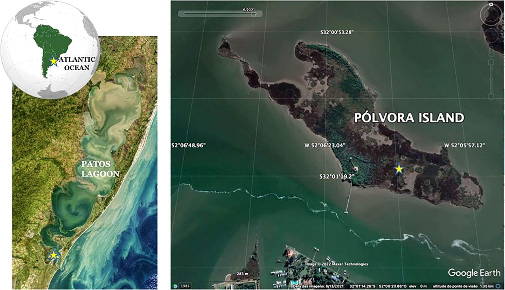
Figure 1 Location of the Patos Lagoon in southern South America and Pólvora Island in Patos Lagoon Estuary. The study site is represented by the yellow star in the consecutive maps. (left) Landsat 8 (OLI) image of Patos Lagoon of 24 May 2018 provided by NASA Earth Observatory. (right) Pólvora Island image of 13 June 2021 provided by Google Earth Pro®.
The regions climate is subtropical humid (Cfa) according to Koeppen-Geiger criteria (Reboita and Krushe, 2018), with four distinct seasons and average maximum temperature in January of 24.2°C and an average minimum temperature of 13.2°C in July. The annual precipitation is around 1360 mm distributed over all months, although the winter period presents a slightly higher precipitation (120-130 mm/month) compared to the summer (90-100 mm/month). The increased rainfall in winter is due to the more frequent penetration of atmospheric systems (cold fronts) to this region. These systems bring cold air masses and are associated with several meteorological phenomena such as frontal systems crossing the area from the Pacific Ocean, cold fronts and cyclones developed in southern Brazil or in the vicinity and atmospheric blocking, among others (Reboita et al., 2010).
The annual cycle of sunshine hours is from 10 h (winter) up to 14 h (summer). The ENSO events also influence the precipitation, with El Niño (La Niña) producing higher (lower) precipitation with respect to the climatological average at a determined period (Silva et al., 2021). For our data collection period (July 2016 up to April 2017), a moderate La Niña1 event occurred from July until December, inducing lower precipitation than the normal climatological values.
Micrometeorological measurements
In order to take the vegetation/soil-atmosphere CO2 flux data used here, a 3 m tall, micrometeorological tower was installed in January 2016 (32° 01’17.08’’S, 52° 06’10.20’’W) in Pólvora Island (Supplementary Figure 1). The installation and maintenance of the tower and sensors was a multi-institutional effort carried out between (1) the Center for Weather Forecast and Climate Studies (CPTEC) of the National Institute for Space Research (INPE); (2) the Institute of Oceanography (IO) and the Oceanographic Museum Prof. Eliézer de Carvalho Rios of the Federal University of Rio Grande (FURG); and (3) the State Center for Remote Sensing and Meteorology Research (CEPSRM) of the Federal University of Rio Grande do Sul (UFRGS). After installation, the tower was fully operational with all sensors operating from July 2016 to April 2017, apart from a week in October 2016 (due to battery failure) and from mid-November to the end of December 2016 when sensors were being serviced. Precipitation data were not collected due to a failure on the rain gauge electronics. Sensors were periodically serviced at about every 3-months period, mainly for cleaning, and no dataset was found to drift from the expected range of measurements during the time of our experiment.
Although the island’s topography is flat and very close to the water level, subjecting the terrain to periodical flooding (Costa, 1997a; Costa and Marangoni, 2010), the tower’s position in the high-mid marsh avoided water suppressing the vegetation at the site during our study period.
Supplementary Table 1 provides a list of sensors used in the tower. Most of sensors operated in the 30 s period (1/30 Hz frequency) but the IRGASON (Campbell Scientific Corporation, Logan, Utah, USA), an integrated 3D sonic anemometer with and open path gas analyzer operated at the 10 Hz frequency necessary for the EC estimates. The IRGASON has also a thermometer and a barometer to make auxiliary measurements at the same frequency as the wind and gas concentration.
As suggested by Verbeeck et al. (2011), the chosen position for the tower installation suitable for EC measurements, lying on very flat terrain that extends about 1,500 m in the northwestern/southeastern direction by about 200 m in the northeastern/southwestern direction (Supplementary Figure 2). The tower’s location lies on an area dominated by Spartina densiflora (Supplementary Figure 3). The shortest distance between the tower’s position in Pólvora Island and Rio Grandes’s city center is 700 m. As the island is located north of the city and prevailing winds during our experiment were from the northeastern/eastern quadrants (Supplementary Figure 4) where there are no settlements, we do not expect significant urban contamination of our CO2 measurements.
In order to estimate the source area and the contribution of a specific target to the surface/atmosphere fluxes, footprint (or fetch) models are used in association with the EC measurements. In this paper, we used the 2D footprint model described by Kljun et al. (2004) and Kljun et al. (2015) and freely available by the Tovi™ s. The software uses meteorological information like windspeed and direction, surface turbulent fluxes (especially momentum and sensible heat fluxes), the atmospheric stability estimate (including the Monin-Obhukov Length), and information of the vegetation like height, displacement heights and roughness length. In our case, although these parameters vary with the seasonal cycle (Costa et al., 2003), we found that the roughness parameter variation up to a value of 1 m did not affect the calculation of the footprint area. Using the extremely high roughness parameter of 1 m, the footprint was computed as between 200-300 m (area of ~0.25 km-2) for both winter-spring and summer-fall periods (Supplementary Figure 5). As we observed spatial homogeneity of the salt marsh vegetation in all directions around the instrument tower for both study periods, we assumed that all CO2 flux measurements presented in this work were solely related to the salt marsh vegetation and represent its typical behavior.
As conventionally needed for the EC calculations, the original (3 m height) windspeed measured by the IRGASON 3D sonic anemometer was converted into its 10 m height equivalent (U10) using the Coupled Ocean-Atmosphere Response Experiment (COARE) version 3.5 bulk algorithm (Edson et al., 2013). The atmospheric pressure data collected by the IRGASON barometer were extremally noisy from March 15, 2017 onward and they were not used here. The original data collected at 3 m height were also converted into sea level pressure (SLP, 0 m height) in a similar way. Both conversions make our data easily compared in the future to most atmospheric datasets in the world.
Auxiliary environmental data: water level, precipitation and wind
In order to assess the relations between water level and the micrometeorological measurements made throughout the study period, we used water pressure (proxy to water level) data gathered by the Laboratory of Coastal and Estuarine Oceanography (LOCOSTE) of IO-FURG during the period of this study. Water pressure data were taken by a thermo-condutivimeter (CT) SeaBird SBE 37-SM moored in the estuary’s mouth about a kilometer away from the Pólvora Island in a depth between 4.5 and 5 m. The instrument provided a pressure mean (4.63 dbar) over the 2-years time period. This 2-years mean value was subtracted from the daily means to provide the water pressure anomaly (WPA) data used here.
As precipitation data was not directly collected by the rain gauge installed in the micrometeorological tower, we used data from the Brazilian National Institute of Meteorology (INMET)2 available for the period of this study. INMET maintains the automatic weather station #A802 (a.k.a. 83995) in Rio Grande city at the position 32°04’43” S; 52°10’03” W inside the Federal University of Rio Grande (FURG) at a distance of around 9 km from the site of our micrometeorological tower. The data presented many gaps making its use as a robust time series impossible. Nonetheless, we used the data to characterize the synoptic meteorological conditions of the study area.
In order to investigate the climatology of the wind field of our study area, we used hourly values (not shown) from a meteorological reanalysis database provided by the European Centre for Medium Range Weather Forecast (ECMWF) named ERA53. It uses a 4D variational assimilation scheme (Hersbach et al., 2020). Briefly, ERA5 consists of hourly atmospheric variables computed at a ~30 km grid size for more than 130 height levels in the atmosphere from the Earth’s surface up to 60 km. The wind data used here were extracted from the grid point including Rio Grande city (32°S, 52 °W) for the period from 2010-2020 at 100 m height in the atmosphere. The analysis of these data (not shown) indicated that during our study period the winds were close to the climatological means for each of the seasons.
Eddy covariance estimates of CO2 fluxes
The eddy covariance method correlates the turbulent fluxes of a determined scalar between two determined environments, for instance the interface of surface (vegetation/soil/water) and the atmosphere. The parameters are measured by sensors installed in micrometeorological towers and are used to estimate the net exchanges of CO2, water and energy between the surface and the atmosphere (Stull, 1988; Jung et al., 2011; Edson et al., 2013). The EC method measures the covariance between the turbulent fluctuations of a scalar and vertical windspeed around their mean during a determined sampling interval. For instance, here we use a sampling frequency of 10 Hz for the fast response sensors and a time interval of 30 min for the computation of the fluxes. The high frequency fluctuations correspond to measurements of the transport of energy by the small atmospheric eddies. The time interval window (e.g. 30 min) data is then computed in order to resolve and include the transport by the large-scale eddies (Kaimal and Finnigan, 1994; Miller et al., 2010).
Using the IRGASON, we measured the 3D wind velocity vector components (u, v, w) and the density of H2O(v) and CO2 in order to calculate their mixing ratio (H2O(v)/CO2) in the atmosphere to further calculate the turbulent CO2 EC fluxes (FCO2 in μmol m−2 s−1) at the vegetation/soil-atmosphere interface as:
where, ρa is the dry air density, w is the vertical component of the wind velocity and c is the mixing ratio (e.g. H2O(v)/CO2) The means are represented by over bars and the turbulent fluctuations are represented by the primes. All data were processed using the open source software EddyPro® v.6.2.14. At this step, we configured the proper corrections for flux computation as wind rotation, planar fit, corrections for air temperature, atmospheric pressure and humidity etc (Webb et al., 1980; Miller et al., 2010; Aubinet et al., 2012). EddyPro® follows the scheme proposed by Foken et al. (2004) for the data quality-control. Necessary spectral corrections were made for both low- and high-frequency bands following the methods described by Moncrieff et al. (2004). The statistical tests used to clear spikes on the micrometeorological time series were performed according to Vickers and Mahrt (1997) using 30 min long time intervals and detrended time series derived from the original data. The methodology used here is similar to that used by Oliveira et al. (2019); Santini et al. (2020) and Pezzi et al. (2021).
Once the CO2 fluxes were computed for the two periods of this study, we used the synchronized radiation series to separate the data into daytime (from about 6 a.m. up to 18 p.m. local time) and nighttime series (from about 18 p.m. up to 6 a.m. local time), from which we calculated the basic statistics (mean and standard deviation) for both daily periods. Then we computed the net CO2 fluxes to assess the role of the salt marsh environment as a sink (negative net fluxes) or a source (positive net fluxes) of CO2 to/from the atmosphere. Using only the daily values of minimum (nighttime) and maximum (daytime) values, we also computed the maximum daily amplitude of the CO2 fluxes and statistics of the series at the monthly scale and for the two periods analyzed here (winter-spring and summer-fall).
Wavelet and cross-wavelet analysis
A wavelet transform was used to determine the temporal variability of the CO2 fluxes and to estimate the coefficients of cross-correlations (r) between these fluxes and atmospheric and water level variables. From all meteorological variables collected by the instrument tower, the following were used for the analysis: air temperature, relative humidity and windspeed. Apart from correlating the fluxes with the meteorological variables and water level anomaly, we also correlated the water level with windspeed to support the assumption that these variables are highly correlated (Möller et al., 2001). All variables were averaged to a daily temporal resolution before the analysis.
The cross-wavelet analysis and wavelet coherence were performed according to the methodology proposed by Grinsted et al. (2004). We used a cone of influence (p>0.05) to separate valid data from the red noise. Briefly, the cross-wavelet spectrum analysis emphasizes the common power of the two-time series, while the wavelet coherence emphasizes the correlations between temporal cycles imprinted on two time series, e.g, the coherence fluctuations. We thus determine the local correlation of significant oscillations observed among the CO2 EC fluxes and environmental variables. We used the software STATISTICA7.0® to perform the cross-correlations and Matlab7.0® to perform the wavelet and cross-wavelet computations.
Results
Salt marsh-atmosphere CO2 fluxes and associated environmental variables
Figures 2, 3 present the time series of CO2 fluxes at the salt marsh-atmosphere interface and the environmental variables SLP, air temperature and water level anomaly for the two sampling periods of this study (July-November 2016 and January-April 2017, respectively). Supplementary Figures 6 ,7 present the time series of windspeed, relative humidity, incoming shortwave radiation and precipitation for the different study periods.
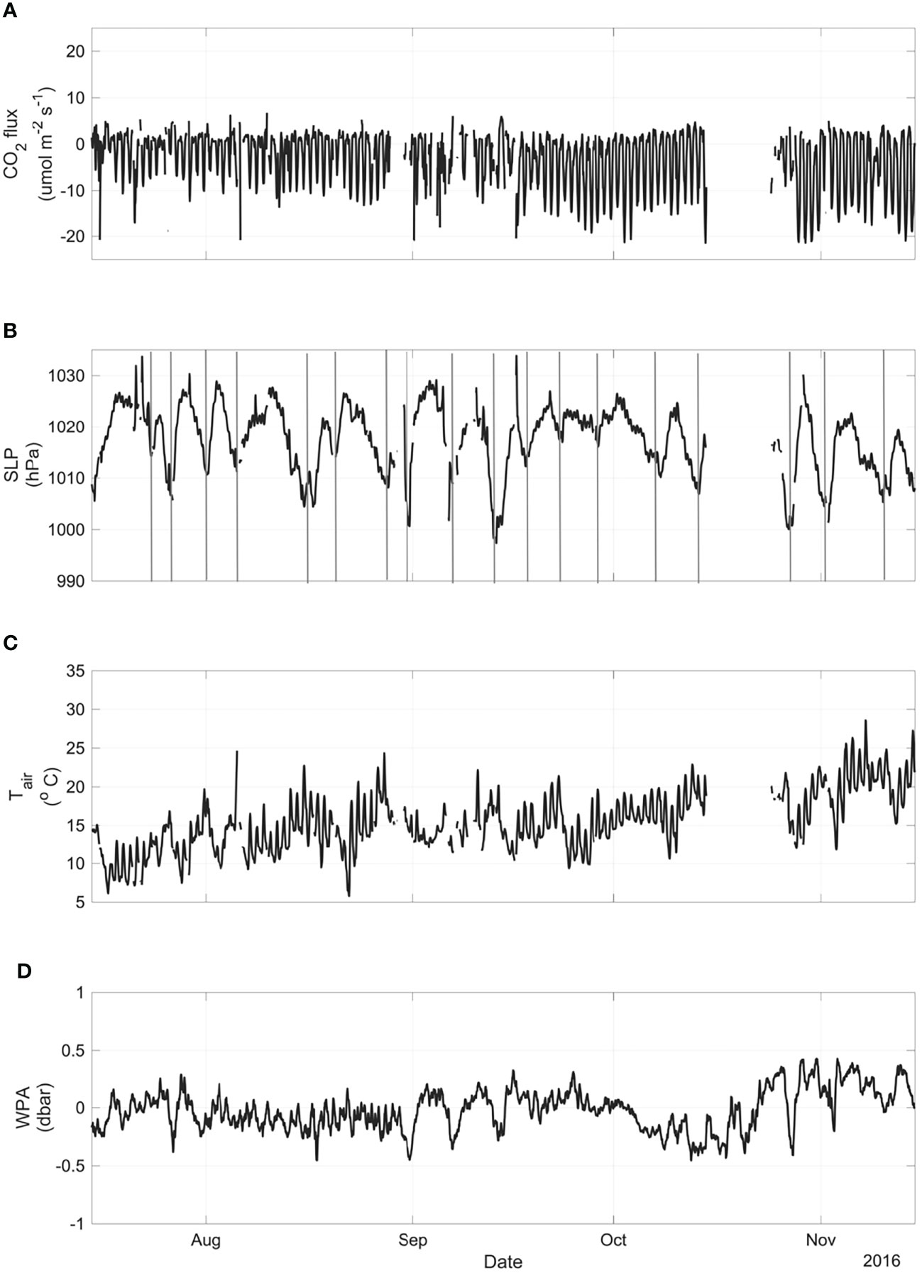
Figure 2 Time series of (A) CO2 fluxes at the salt marsh-atmosphere interface; (B) sea level pressure (SLP); (C) air temperature (Tair); (D) water pressure anomaly (WPA) for the period spanning from July up to November 2016. The vertical gray lines in (A) indicate the pressure troughs associated with the passage of atmospheric cold fronts in the study area.
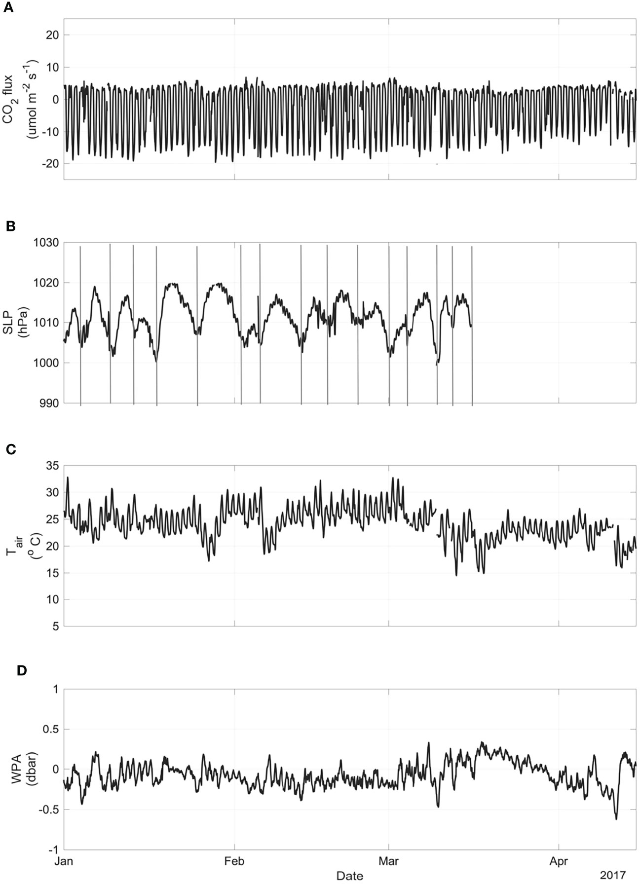
Figure 3 Time series of (A) CO2 fluxes at the salt marsh-atmosphere interface; (B) sea level pressure (SLP); (C) air temperature (Tair); (D) water pressure anomaly (WPA) for the period spanning from July up to November 2016. The vertical gray lines in (A) indicate the pressure troughs associated with the passage of atmospheric cold fronts in the study area.The mean values of net CO2 flux are negative and almost the same for both periods of this study (-3.23 to -3.20 μmol m-2 s-1) (Table 1). Mean value of night fluxes (a proxy of community respiration) is about 4.6 times higher in summer-fall than in winter-spring (Table 1). Daytime mean fluxes, related to the community photosynthetic activity, varied between (-6.71 to -7.95 μmol m-2 s-1) between the two periods analyzed. The mean value of nighttime fluxes, on the other hand varied between 0.67 (winter-spring) to 2.95 μmol m-2 s-1 (summer-fall). Variability in mean values of CO2 fluxes is higher during daytime when compared to the nighttime measurements, for both periods (Table 1), following the high variability in the incoming shortwave radiation, a variable dependent on the cloudiness (Supplementary Figures 6C, 7C).
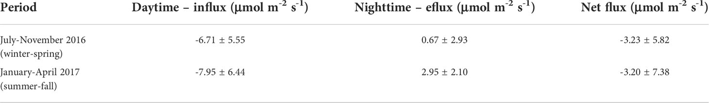
Table 1 Mean (± standard deviation) values of salt marsh-atmosphere CO2 flux during daytime, nighttime and daily cycle net balance, for both studied periods.
The CO2 fluxes show a typical diurnal cycle, for both winter-spring and summer-fall periods (Figures 2A, 3A). This daily cycle, which is related to the photosynthetic activity and the community respiration, dominates the temporal modulation of the series. It is also noticeable that, for both study periods, the amplitudes of the daytime periods’ CO2 absorption (negative fluxes - influx) are larger than that released during nighttime periods (positive fluxes - eflux), suggesting a positive net balance of photosynthetic activity over the community respiration.
The average maximum negative and positive values of the CO2 fluxes observed, respectively, during daytime and nighttime along the temporal series represent the daily amplitudes of the salt marsh-atmosphere CO2 fluxes (Table 2). The values are a proxy of the maximum photosynthetic rates (daytime negative values) and community respiration (nighttime positive values) for each month during the two studied periods. The peaks of negative (-16.38 to -16.57 μmol m-2 s-1) and positive values (4.39 to 4.92 μmol m-2 s-1) of CO2 fluxes occurred during austral summer (January-February 2017), therefore resulting in the highest amplitudes between day and night (20.77 to 21.49 μmol m-2 s-1). The amplitudes of the CO2 fluxes signal are larger during summer (January-February) than during the winter (July-August), while the fluxes’ variability is lower in summer months.
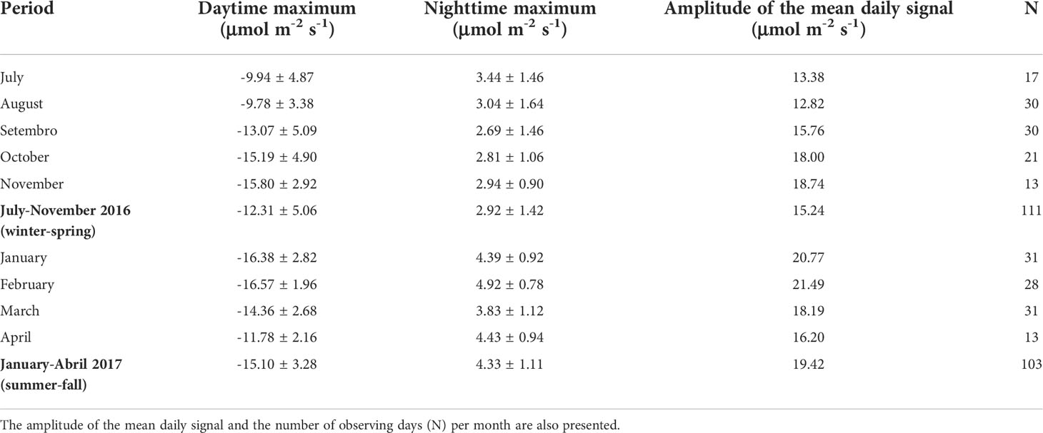
Table 2 Mean and standard deviation for the daytime (nighttime) monthly average of maximum (minimum) values of the CO2 flux measured during both study periods.
Using Table 1 data for the net CO2 seasonal fluxes, the annual average of the CO2 taken up by the salt marsh can be estimated as -3.215 μmol CO2 m-2 s-1 or -3.215 x 10⁻⁶ mol CO2 m-2 s-1. Considering that the mass of carbon in a mol of CO2 is 12 g and applying the correct transformations of units, this results in a theoretical fixation tax of carbon close to -1217 g C m-2 yr-1. Extrapolating this value for the total extension of the Patos Lagoon salt marshes (72 km2; Nogueira and Costa, 2003) gives us an annual carbon fixation rate for the entire area covered by the Patos Lagoon marshes close to -87.6 x 10⁹ g C yr-1 (-87.6 Mg C yr-1).
Some of the CO2 flux cycles seen in Figures 2A, 3A follow the cycles presented by the environmental variables studied here. The sea level pressure time series, for instance, show a clear temporal variability in the scale of 3-7 days (Figures 2B, 3B), in agreement with the characteristics of the passage of atmospheric synoptic systems alternating high and low pressures over time. The frequencies of occurrence of high-pressure systems were higher in the winter-spring period (Figure 2B) than in the summer-fall period (Figure 3B) making the amplitude of the pressure differences during episodes of frontal passage in summer-fall (1000 to 1023 hPa) greater than winter-spring (1000 to 1020 hPa).
The air temperature (Figures 2C, 3C), relative humidity (Supplementary Figures 6B, 7B) and the incoming shortwave radiation (Supplementary Figures 6C, 7C) are clearly modulated by the diurnal cycle. As expected for our study area, relative humidity reaches 100% more frequently during the winter-spring period than during the summer-fall. The water pressure anomalies (Figures 2D, 3D) also show a clear diurnal cycle in both study periods and generally follow the atmospheric pressure variability at the synoptic scale. The precipitation data provided by INMET (Supplementary Figures 6D, 7D) show that episodes of heavy rainfall with values of more than 20 mm h-1 are common in Rio Grande city, especially during the summer-fall period.
Windspeed at 10 m height (U10) time series present cycles that are clearly related to the variability of the atmospheric transient systems, as both variables describe the fluctuations related to the atmospheric systems’ passage in our study area (Supplementary Figures 6A, 7A). The wind, though, has a prominent diurnal component, probably related to the sea breeze. Windspeed values are often smaller than 5 m s-1 but sometimes reach more than 10 m s-1 in bursts or gusts related to low pressures occurring in winter-spring. ERA5 climatology for Rio Grande city (not shown) revealed that the windspeed presents a clear seasonal variation and it is stronger (around 8.2 m s-1) during winter than during summer (7.3 m s-1). Also, the more frequent wind direction is usually from NE-E during summer, albeit some events from NW-W also occur during winter. This is also observed in the wind data provided by the micrometeorological tower (Supplementary Figures 4, 6A, 7A).
Wavelet and cross-wavelet analysis
The results of time series analysis (wavelet and cross-wavelet) made clear the dominant period cycles of the studied variables CO2 fluxes, windspeed and water pressure anomaly (Figures 4–7). As previously observed in the original time series (Figures 2A, 3A), CO2 fluxes in the interface salt marsh-atmosphere show a marked diurnal cycle (~ 24h). Our wavelet results indicate that the diurnal cycle accounts for the highest energetic spectral content of our CO2 fluxes time series in both periods of this study (Figures 4A and 6A). The same diurnal cycle was observed in the other variables, although not very well distributed in time and not energetic (Figures 4B, C, 6B, C). The CO2 fluxes, windspeed and water pressure anomaly present significant energy periods centered at 64 to 512 hours (~3 to 21 days), which are associated with the synoptic atmospheric scales (gray lines) seen in Figures 2B, 3B.
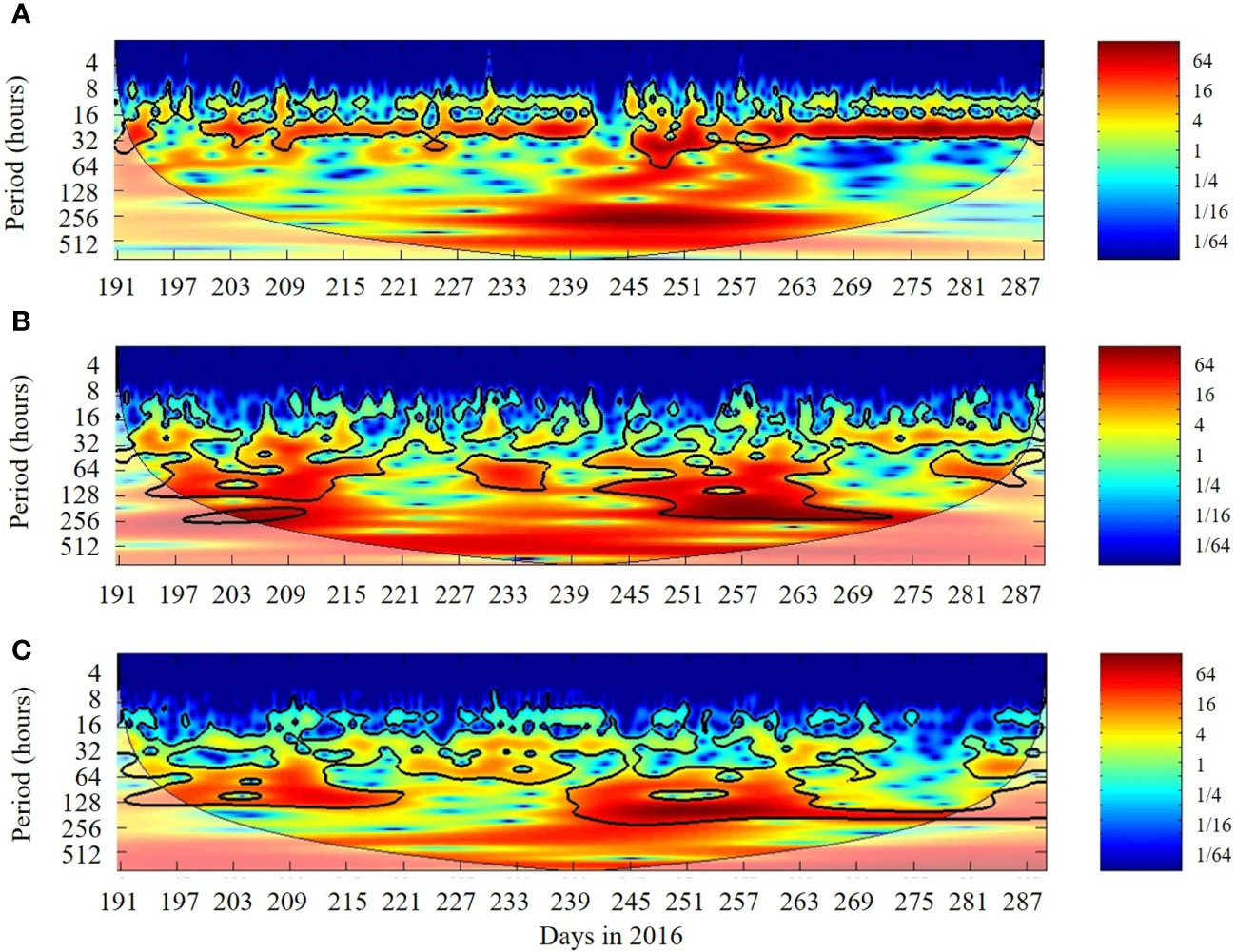
Figure 4 Wavelet power spectrum of CO2 fluxes (A), windspeed (B) and water pressure anomaly (C) for the period spanning from July up to November 2016. The contours are for variance units. The 5% significance level against red noise is shown as a thick contour (cone of influence). Blurred regions indicate values outside the cone of influence. The 95% significance level is shown by heavy black contours. The horizontal scale represents the Julian days in July-November 2016 period. The results of the cross-wavelet analysis for the winter-spring (Figure 5) and summer-fall periods (Figure 7) are presented as the common power (energy) spectrum of the two-time series or the wavelet coherences that emphasize the correlations between variations of two series, i.e., coherence fluctuations. The analysis indicates the local correlation (0 ≤ r ≤ 1) of significant oscillations observed between the CO2 fluxes and windspeed and water pressure anomaly. The relative phase between the variables is presented as vectors: they point toward the right (left) at the horizontal when the variables are totally in phase (out of phase).
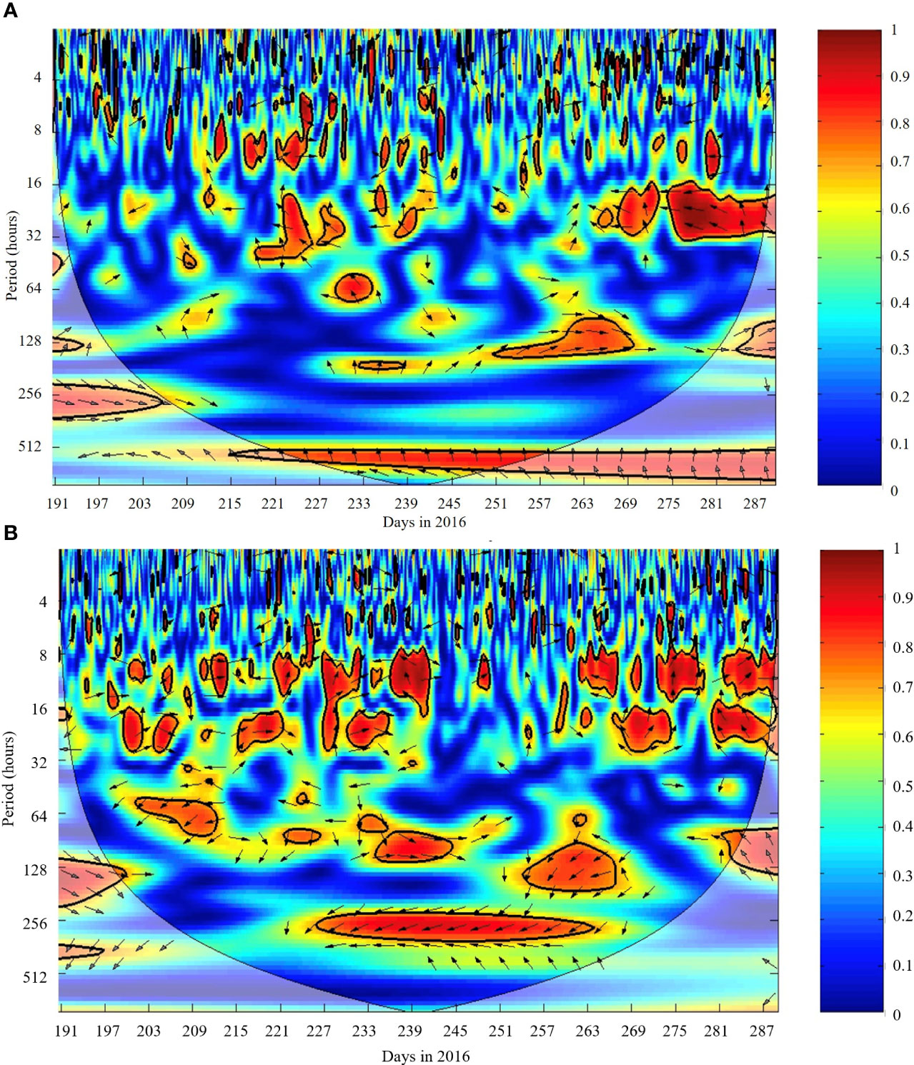
Figure 5 Cross-wavelet coherence of CO2 fluxes and windspeed (A) and CO2 fluxes and water pressure anomaly (B) for the period spanning from July up to November 2016. The contours are for variance units. The 5% significance level against red noise is shown as a thick contour (cone of influence). Blurred regions indicate values outside the cone of influence. The vectors indicate the relative phase between the variables. The horizontal scale represents the Julian days in July-November 2016 period.
Figure 6 Wavelet power spectrum of CO2 fluxes (A), windspeed (B) and water pressure anomaly (C) for the period spanning from January up to April 2017. The contours are for variance units. The 5% significance level against red noise is shown as a thick contour (cone of influence). Blurred regions indicate values outside the cone of influence. The 95% significance level is shown by heavy black contours. The horizontal scale represents the Julian days in January-April 2017 period.
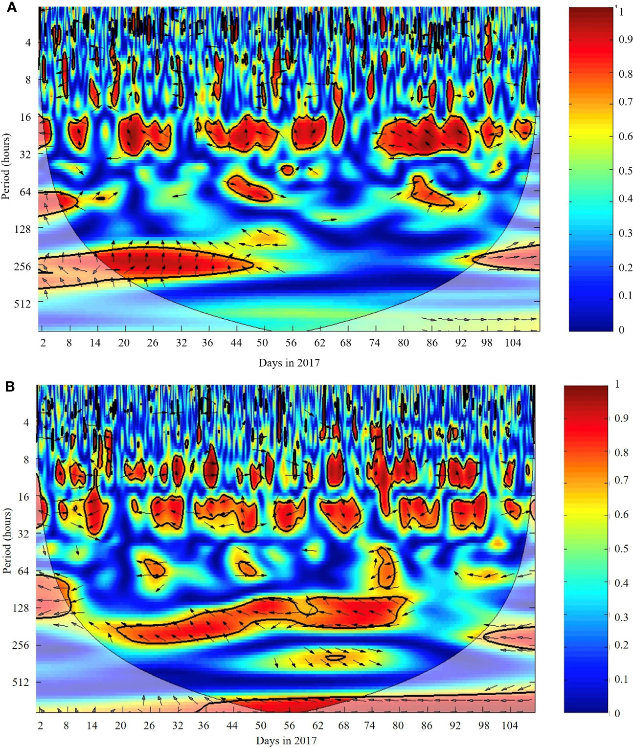
Figure 7 Cross-wavelet coherence of CO2 fluxes and windspeed (A) and CO2 fluxes and water pressure anomaly (B) for the period spanning from January up to April 2017. The contours are for variance units. The 5% significance level against red noise is shown as a thick contour (cone of influence). Blurred regions indicate values outside the cone of influence. The vectors indicate the relative phase between the variables. The horizontal scale represents the Julian days in January-April 2017 period.
Figures 5 and 7 present highly coherent, cross-energy peaks are scattered between semi-diurnal or diurnal cycles (~12 to 24 h) and low-frequency ones, mostly between 64 to 512 hours (~3 to 21 days) as already seen in the individual power spectra (Figures 4 and 6). The semi-diurnal coherences are in phase, showing that the CO2 fluxes directly respond to both windspeed and water pressure anomaly. Episodes of high correlations, however, were not continuous throughout the entire time series, but rather associated to episodes of high amplitude of the variables involved.
A noticeable episode of high cross-energy between CO2 fluxes against windspeed and water pressure anomaly centered at 128 hours (~5.33 days) occurred between Julian days ~250 to ~270, corresponding to 6 to 26 September 20165 (Figure 5) coincided with a period of high water pressure anomalies (~ 10 dbar) recorded by the CT instrument located in the Patos Lagoon Estuary (Figure 2D). At the same period, windspeed was relatively low, ranging between 3-6 m s-1 (Supplementary Figure 6A). The cross-wavelet coherence of CO2 fluxes against windspeed is very high and in phase during the period of Julian days ~250 to ~270 (Figure 5A) while the coherence between CO2 fluxes and water pressure anomaly for the same period, although still high, is out of phase (Figure 5B).
The cross-wavelet results between CO2 fluxes and windspeed shows two high-coherence, in phase peaks centered at about 64h (~3 days) in periods ranging from Julian days 40-50 (9-19 February 2017) and Julian days 80-90 (21-31 March 2017 - Figure 7A). Other peak in Figure 7A occurs at the ~265 hours period (~11 days) during Julian days 20-40 (20 January to 9 February 2017). The variables were time-lagged at about 3 days (a quarter of a 11-day cycle).
The cross-wavelet coherence spectra of CO2 fluxes and water pressure anomaly (Figure 7B) shows a prominent out of phase, high-coherence peak centered at about 192h (8 days) in periods ranging from Julian days 20-80 (20 January to 21 March 2017). During this period the water level anomaly, albeit positive, was about 5 dbar lower that the subsequent period - fall (Figure 3D).
Discussion
The present study is, to our knowledge, the first to measure gas exchange in a Brazilian saltmarsh ecosystem. Our results suggest that subtropical salt marsh habitats are net sinks of carbon. Our study also described the different temporal scales dominating of the salt marsh-atmosphere CO2 flux cycles, emphasizing the control of the diurnal cycle by aspects linked to the plant’s physiology and the control of longer periods’ cycles by environmental factors.
The salt marsh-atmosphere CO2 EC fluxes measured in Pólvora Island presented a clear cycle at the diurnal scale during all seasons of our study in 2016-2017, forced by the balance between photosynthesis (negative fluxes) and community respiration (positive fluxes). The mean daytime fluxes were -6.71 ± 5.55 μmol m-2 s-1 (-7.95 ± 6.44 μmol m-2 s-1) for the winter-spring (summer-fall) season. During nighttime, the mean CO2 fluxes were 0.67 ± 2.93 μmol m-2 s-1 (2.95 ± 2.10 μmol m-2 s-1) in winter-spring (summer-fall). Although there is high variability in the data, the effectiveness of the salt marsh as a CO2 sink was attested by the computation of the net CO2 balance with a predominance of the photosynthetic activity over respiration and net flux of about 3.2 μmol m-2 s-1 throughout the period of this study.
Our results showed a clear seasonal cycle, with differences of CO2 fluxes between winter and summer (Tables 1, 2). This pattern is similar to what found by Tonti et al. (2018), for EC measurements taken in a salt marsh in Argentina (about 38° S) in 2014. These authors related the summer uptake increase of CO2 by the salt marsh vegetation to both the increase of the air temperature and the duration of the day, consequently increasing the photosynthetic activity in that season. In agreement to the range of results presented in this work (Table 2), Tonti et al. (2018) reported a -12.9 μmol m-2 s-1 uptake peak during daytime in March 2014. During daytime in winter, on the other hand, the CO2 uptake by the vegetation was lower than in summer, peaking at -4.6 μmol m-2 s-1 in August 2014. The results of both studies suggest that the seasonal cycle of air temperature, daylength (light) and plant responses are important forcing mechanisms for the vegetation-atmosphere annual CO2 flux amplitudes in Southwestern Atlantic salt marshes. The annual fixation rate of carbon in this ecosystem, estimated as -1217 g C m-2 yr-1, represents the amount of carbon fixed from the atmosphere in the plant and not necessarily sequestrated by the plant for growth and/or deposited in the sediment. Nevertheless, this fixation rate is about 5 times the mean carbon uptake of salt marshes in other locations (i.e. mean of -245 g C m-2 yr-1, Ouyang and Lee, 2014).
The existing knowledge of CO2 fluxes between the vegetation and the atmosphere in Brazil are restricted to terrestrial biomes. A recent study reported the seasonal behavior of the gross primary production (GPP) - a variable directly related to the fluxes - in four terrestrial biomes: Pantanal, Amazonia, Caatinga and Cerrado (Costa et al., 2022). Analyzing data from one particular location in each biome in distinct periods ranging from 2004 to 2016, the authors described how the seasonal cycle of meteorological variables such as the global incident radiation, air temperature and water vapor deficit, as well as precipitation were the key modulating factors of seasonality in GPP for all biomes.
Armani et al. (2020) presented a study of the EC CO2 and heat fluxes measured in a reservoir located in the Paraná River, southern Brazil, during 2013. The micrometeorological instruments were deployed in a tower installed in one of the reservoir’s islands which is flat and almost submerged, located at 25°03’25.72’’ S, 54°24’33.67’’ W. The authors reported remarkable seasonality of the CO2 fluxes: in the warm season, the CO2 fluxes were negative (CO2 uptake by the vegetation) during daytime due to photosynthesis and positive (CO2 emittance by the vegetation) at nighttime due to the respiration activity. This result agrees with our findings and supports the idea that the plant’s physiology is the major driver of the vegetation/atmosphere CO2 fluxes. During the cold season, however, Armani et al. (2020) found that both daytime and nighttime CO2 fluxes were predominantly negative, suggesting an imposition of the atmosphere’s CO2 concentration and the occurrence of stronger winds on the CO2 fluxes. The authors also reported that 90% of the CO2 flux measurements made in their study area ranged between -102.68 to 151.72 μmol m-2 s-1. In average, the CO2 flux was 12.78 μmol m-2 s-1, indicating that the reservoir was a source of CO2 to the atmosphere.
The amplitudes of the salt marsh-atmosphere CO2 fluxes’ diurnal cycle for both study periods seen in Figures 2A, 3A demonstrate that they were modulated by the passage of transient atmospheric systems, such as cold fronts, and by the level variation of the island’s surrounding waters. Beside the seasonal changes in sunlight (daylength) and air temperature, differences between the spring-summer and winter-fall periods are marked by the variation in the level of marsh inundation that is usually higher in winter-spring months than in the summer. The salt marsh inundation is locally driven by the Patos Lagoon discharge and windspeed which tend to be higher in winter.
The time series of the meteorological variables collected in our study area (Figures 2, 3 and Supplementary Figures 6, 7) attest the predominance of both the seasonal variability and the short-term, synoptic scale (3 to 7 days) events in our study area. The sea level pressure (Figures 2B, 3D) and windspeed data (Supplementary Figures 6A, 7A) clearly show the cycles related to the passage of atmospheric synoptic systems during both study periods. In addition, the diurnal cycle is also prominent in these time series and particularly visible in the air temperature series (Figures 2C, 3C). The seasonal cycle is very clear, as expected, in the air temperature series with values generally above 20°C from November 2016 onwards.
Using precipitation data of Rio Grande city in the period 1913-2016, Silva et al. (2021) describe that the monthly means of this variable are uniformly distributed along the year without distinguishable dry and wet seasons. On analyzing the period 1950-1980, however, the authors noticed that the summer-fall season was dryer, and the winter was wetter than during the whole period 1913-2016. Wetter summers, including the month of November, were predominant during the period 1980-2010. Silva et al. (2021) also report that the major modes of variability of the precipitation in Rio Grande, which can be extrapolated to the study area, are related to the seasonal cycle and to a ~5-years and a 8-years period oscillation linked to the ENSO phenomenon. The authors described that the 5-years (8-years) ENSO cycle is associated to the positive (negative) phase of the Pacific Decadal Oscillation, demonstrating that the teleconnections are important for characterizing the climate of the study area. As described before, during both periods of this study, a moderate La Niña event induced lower precipitation than the normal climatological values. This situation may have produced CO2 fluxes lower than average.
Figures 4–7 show that patterns in winds and water level had strongly influenced our CO2 fluxes. This result corroborates the findings of Möller et al. (2001). The authors studied the subtidal circulation of the Patos Lagoon Estuary analyzing time series of wind, outflow (discharge) and water level collected in situ together with numerical model outputs. They emphasize the importance of the wind forcing in the modulation of the estuary outflow, pointing out to the effects of the passage of meteorological fronts in the temporal scale of 3 to 16 days that produce an inversion of the pressure gradient between the inner and outer parts of the Patos Lagoon. Winds blowing from the southern quadrant produce a pressure gradient from the sea toward the estuary (landward) while northernly winds do the opposite (seaward). Möller et al. (2001) did not report on eventual time lag between the variables, however they pointed out to a phase lag that occurs between the inner Patos Lagoon and the adjacent coastal waters of the South Atlantic Ocean. This lag is modulated by the along-shore (along-estuary) winds and by the morphology of the estuary that acts by filtering tidal and longer period oscillations generated outside the estuary.
Forbrich and Giblin (2015) studied CO2 fluxes using the EC technique between a salt marsh vegetation in New England, USA, and the atmosphere in the months of May to October between 3 years of measurements (2012-2014). They noticed a considerable loss of CO2 transfer in the marsh-atmosphere interface during both night and day under situations of tidal inundation (spring tides at ~15-day periodicity in their case). The authors, using NDVI data estimated from satellites, report areas of low elevation marshes susceptible to suffer reductions in their CO2 fluxes during inundation events.
Although our site in the Pólvora Island is not subject to high tidal amplitudes (Möller et al., 2001) and the precipitation in the vicinity is not very distinct among all seasons when analyzed at the long-term scale (Silva et al., 2021), it is expected that wetter seasons or individual episodes would impact (diminishing) the vegetation/soil-atmosphere CO2 fluxes. As pointed out by Möller et al. (2001), a wetter estuary (marsh) in the vicinity of our study area is related to the increase in the Patos Lagoon outflow (water level) that, on the other hand, is forced by northerly winds and the increase in precipitation, especially during wintertime.
The episode of Julian days ~250 to ~270 (ordinal calendar days 6 to 26 September 2016 - Figure 5) represents a period of very high water pressure anomalies (Figure 2D) and low windspeed (Supplementary Figure 6A) resulting in a very high, in phase (out of phase) cross-wavelet coherence of CO2 fluxes against windspeed (water pressure anomaly), showing that high water levels reduce CO2 uptake in the marsh and corroborating the results from Forbrich and Giblin (2015). Other similar episodes throughout the time series shown in Figure 5B, where the CO2 fluxes are out of phase with the water pressure anomaly, confirm the findings of Forbrich and Giblin (2015) of a negative correlation between water level and salt marsh-atmosphere CO2 fluxes.
The results presented in Table 2 for the amplitudes of the diurnal CO2 fluxes also show that these amplitudes are higher during the dryer season of the summer (January-February) 2017 with respect to the winter (July-August) 2016. It is clear from Table 2 that, during the summer, higher CO2 fluxes occurred during both daytime and nighttime periods. A study using the EC technique in a tropical mangrove (Freire et al., 2022) indicated that the highest values of vegetation-atmosphere CO2 fluxes occurred during the wet season, in contradiction to our results for the Patos Lagoon salt marsh. In both ecosystems, however, the precipitation or water level seem to be major drivers for the vegetation-atmosphere CO2 flux variability.
Krauss et al. (2016) point out that, although salt marshes absorb the atmospheric CO2, these ecosystems also emit CO2 and two other greenhouse gases (CH4 and NO2). Nevertheless, the authors report that the carbon sequester in wetlands is much greater than most ecosystems and, as a consequence, these environments draw general interest as greenhouse gas sinks. Studying the Louisiana (USA) wetlands, Krauss et al. (2016) reported an uptake rate of CO2 by the marshes of -337 g C m-2 yr-1 which is about 3.6 times less than our estimate of -1217 g C m-2 yr-1 for the Patos Lagoon marshes. The authors also offered a comparison between EC measurements of greenhouse gas fluxes and estimates obtained from the more traditional technique of chambers, describing that the different spatial and temporal sampling footprints of the EC and the chambers techniques require further understating to make direct comparisons between these techniques possible.
As all techniques, the EC CO2 flux estimates also present a range of limitations. Oliveira et al. (2019), for instance, described that EC CO2 fluxes are computed using an estimate of the turbulent mixing ratio between the water vapor and the CO2 in the atmosphere that is performed before any calculations of the surface-atmosphere CO2 fluxes. These measurements, along with the original concentrations of these gases in the atmosphere need to be estimated at the same frequency as the vertical component of the wind and all instruments need to be calibrated and frequently serviced, as was the case in this work. At the same time, an accurate dry air density value is necessary in the calculations and a correct setting up of the EddyPro® routines should be applied. Hollinger and Richardson (2005), however, consider that the EC technique the best method to quantify surface to atmosphere fluxes with uncertainties in the order of only 5%.
Conclusion
This work presents the first results of vegetation/soil-atmosphere CO2 flux measurements made using the eddy covariance technique for a salt marsh environment in Brazil. The major findings demonstrate that the local marsh biome is an effective sink for the atmospheric CO2 during both periods of this study: July-November 2016 (characterizing the winter-spring seasons) and January-April 2017 (summer-fall seasons). The amplitude of the daytime (CO2 fixed) and nighttime (CO2 released) fluxes are dependent on the seasons, being higher during the summertime.
Our results also show that the CO2 fluxes in the Patos Lagoon Estuary salt marshes are primary dependent on the diurnal cycle related to the photosynthetic and community respiration processes. For longer time scales, from the atmospheric synoptic cycles to the seasonal cycle, the results demonstrate that the CO2 fluxes are correlated and phase dependent on the winds and water level cycles. Considering the whole area of the Patos Lagoon Estuary salt marshes, this work also offers the first estimate of an annual, area-integrated net CO2 flux indicating the sink of atmospheric CO2 of -87.6 Mg C yr-1 averaged over all seasons. It is important to remember that, although not clearly seen in our data, the second semester of 2016 was a La Niña period, supposing a drier condition for our study area. Our results, in this case, may be overestimated compared to others “normal” years.
The importance of salt marshes is well known, especially when taking into account their role as a source of organic matter and nutrients that support fisheries. The predicted sea level rise imposed by the global warming represents a great risk for these environments (Boorman, 1999). The lower CO2 sink of the salt marsh with higher water levels in the lagoon suggest that sea level rise could result in lower productivity. Although in Brazil the future expected sea level rise is not very well understood, its impacts add onto the negative pressures already imposed by urban expansion in the coastal regions. The past reduction of the salt marsh extent due to urban expansion in the Patos Lagoon Estuary is well documented (Costa, 1997a; Costa, 1997b; Marangoni and Costa, 2009; Seeliger, 2010) and greatly impacts this environment in southern Brazil.
Taking into account the relevance of Patos Lagoon salt marshes for the maintenance of local estuarine fisheries and coastal protection (), the present study provided further basis for the conservation plans and climate change policies. Our work contributes to the present knowledge on the global carbon budget and for the conservation and management of Brazilian coastal wetlands.
Data availability statement
The raw data used in this study can be made available by the authors under request.
Author contributions
RS and MC conceived "the study". RS, MC and GF wrote the manuscritpt. RS, MC and RA provided the infrastructure, equipments and gave the logistic support. MS, WP and FF processed the data and produced most of the figures. MS, RA, OM and LP revised the text. All authors contributed to the article and approved the final version of the manuscript.
Funding
This research was funded by the Brazilian agencies CNPq, CAPES, FINEP and FAPERGS through the following projects: (i) National Institute for Science and Technology of the Cryosphere (CNPq 704222/2009 + FAPERGS 17/2551-0000518-0); (ii) Polar Marine Meteorological Laboratory, Multiusers Equipment INPE 2016 (FINEP 01.16.0076.00); (iii) Use and Development of the BESM Model for Studying the Ocean-Atmosphere-Cryosphere in High and Medium Latitudes (CAPES 88887- 145668/2017-00) and (iv) Brazilian Research Network on Global Climate Change - Rede CLIMA (FINEP 01.13.0353-00). RS, GF, OM and LP. are partly funded by e (Rede CLIMAFINEP/Grant 01.13.0353-00) fellowships of the CNPq Scientific Productivity Program (CNPq/308642/2021-0; CNPq/307048/2018-7; CNPq/4029906/2019-5 and CNPq/304858/2019-6, respectively).
Acknowledgments
The authors acknowledge the Brazilian National Institute of Meteorology (INMET) and the European Centre for Medium Range Weather Forecast (ECMWF) for providing the supplementary meteorological data used here. We thank Prof. Lauro Barcellos, head of the FURG Museum Complex for the support to this project and by providing the access and infrastructures for the field campaigns. We acknowledge the support provided by INPE’s Southern Space Coordination (INPE/COESU, Santa Maria – Brazil), by the Institute of Oceanography of Rio Grande University (IO-FURG, Rio Grande - Brazil) and by the Micrometeorology Group, Physics Department, Federal University of Santa Maria (UFSM, Santa Maria - Brazil) for setting up the micrometeorological tower, for the sensor’s maintenance and for the data recovery. We are especially thankful to Catherine Lovelock and two reviewers for their extensive revisions and recommendations that improved the quality of this paper. We thank Joel Rubert, Eliane Klering and Carlos Fujita for their technical assistance during the field works and for the data pre-processing during all phases of this work. The EddyPro® software is available for download at https://www.licor.com/env/products/eddy_covariance/software.html. The Tovi™ software is available for download at https://www.licor.com/shop/software/tovi/register/.
Conflict of interest
The authors declare that the research was conducted in the absence of any commercial or financial relationships that could be construed as a potential conflict of interest.
Publisher’s note
All claims expressed in this article are solely those of the authors and do not necessarily represent those of their affiliated organizations, or those of the publisher, the editors and the reviewers. Any product that may be evaluated in this article, or claim that may be made by its manufacturer, is not guaranteed or endorsed by the publisher.
Supplementary material
The Supplementary Material for this article can be found online at: https://www.frontiersin.org/articles/10.3389/fmars.2022.892857/full#supplementary-material
Footnotes
- ^ https://origin.cpc.ncep.noaa.gov/products/analysis_monitoring/ensostuff/ONI_v5.php
- ^ https://mapas.inmet.gov.br/
- ^ https://cds.climate.copernicus.eu/cdsapp#!/dataset/reanalysis-era5-single-levels?tab=overview
- ^ http://www.licor.com/env/products/eddy_covariance/software.html
- ^ https://landweb.modaps.eosdis.nasa.gov/browse/calendar.html
References
Armani F. A. S., Dias N. L., Damázio J. M. (2020). Eddy-covariance CO2 fluxes over itaipu lake, southern Brazil. Rev. Bras. Recursos Hídricos 25, e43. doi: 10.1590/2318-0331.252020200060
Aubinet M., Vesala T., Papale D. (2012). Eddy covariance: a practical guide to measurement and data analysis (London: Springer Science & Business Media).
Barr J. G., Engel V., Fuentes J. D., Zieman J. C., O’Halloran T. L., Smith T. J. III, et al. (2010). Controls on mangrove forest-atmosphere carbon dioxide exchanges in western Everglades national park. J. Geophys. Res.: Biogeosci. 115 (G2), G02020. doi: 10.1029/2009JG001186
Boorman L. A. (1999). Salt marshes – present functioning and future change. Mangroves Salt Marshes 3, 227–241. doi: 10.1023/A:1009998812838
Chmura G. L., Anisfeld S. C., Cahoon D. R., Lynch J. C. (2003). Global carbon sequestration in tidal, saline wetland soils. Global Biogeochem. Cycles 17 (4), 1111. doi: 10.1029/2002GB001917
Chu X., Han G., Wei S., Xing Q., He W., Sun B., et al. (2021). Seasonal not annual precipitation drives 8-year variability of interannual net CO2 exchange in a salt marsh. Agric. For. Meteorol. 308, 108557. doi: 10.1016/j.agrformet.2021.108557
Costa C. S. B. (1997a). “Tidal marshes and wetlands,” in Subtropical convergence environments: the coast and sea in the southwestern Atlantic. Eds. Seeliger U. Odebrecht C., Castello J. P. (Berlin: Springer Science & Business Media), 24–26.
Costa C. S. B. (1997b). “Irregularly flooded marginal marshes,” in 1997: Subtropical convergence environments: the coast and sea in the southwestern Atlantic. Eds. Seeliger U., Odebrecht C., Castello J. P. (Berlin: Springer Science & Business Media), 73–77.
Costa C. S. B., Marangoni J. C. (2010). “The salt marsh communities,” in 2010: The patos lagoon estuary – a century of transformations. Eds. Seeliger U., Odebrecht C. (Berlin: Rio Grande: FURG), 125–133.
Costa C. S., Marangoni J. C., Azevedo A. M. (2003). Plant zonation in irregularly flooded salt marshes: relative importance of stress tolerance and biological interactions. J. Ecol. 91 (6), 951–965. doi: 10.1046/j.1365-2745.2003.00821.x
Costa G. B., Santos e Silva C. M., Mendes K. R., dos Santos J. G. M., Neves T. T. A. T., Silva A. S., et al. (2022). WUE and CO2 estimations by eddy covariance and remote sensing in different tropical biomes. Remote Sens. 14, 3241. doi: 10.3390/rs14143241
Duarte C. M., Losada I. J., Hendriks I. E., Mazarrasa I., Marbà N. (2013). The role of coastal plant communities for climate change mitigation and adaptation. Nat. Climate Change 3 (11), 961–968. doi: 10.1038/nclimate1970
Duarte C. M., Middelburg J. J., Caraco N. (2005). Major role of marine vegetation on the oceanic carbon cycle. Biogeosciences 2 (1), 1–8. doi: 10.5194/bg-2-1-2005
Edson J. B., Jampana V., Weller R. A., Bigorre S. P., Plueddemann A. J., Fairall C. W., et al. (2013). On the exchange of momentum over the open ocean. J. Physical Oceanography 43, 1589–1610. doi: 10.1175/JPO-D-12-0173.1
Foken T., Göckede M., Mauder M., Mahrt L., Amiro B. D., Munger J. W. (2004). Post-field data quality control Handbook of micrometeorology. a guide for surface flux measurements. Eds. Lee X., Massman W. J., Law B. E. (Berlin: Springer Science & Business Media), 181–208.
Forbrich I., Giblin A. E. (2015). Marsh-atmosphere CO2 exchange ina new England salt marsh. J. Geophys. Research:Biogeosci. 120, 1825–1838. doi: 10.1002/2015JG003044
Freire A. S. C., Vitorino M. I., de Souza A. M. L., Germano M. F. (2021). Analysis of the energy balance and CO2 flow under the influence of the seasonality of climatic elements in a mangrove ecosystem in Eastern Amazon. Int. J. Biometeorol. 66, 347–359. doi: 10.1007/s00484-021-02224-8
Gibbs H. K., Brown S., Niles J. O., Foley J. A. (2007). Monitoring and estimating tropical forest carbon stocks: making REDD a reality. Environ. Res. Lett. 2 (4), 045023. doi: 10.1088/1748-9326/2/4/045023
Goulden M. L., Litvak M., Miller S. D. (2007). Factors that control typha marsh evapotranspiration. Aquat. Bot. 86 (2), 97–106. doi: 10.1016/j.aquabot.2006.09.005
Grinsted A., Moore J. C., Jevrejeva S. (2004). Application of the cross wavelet transform and wavelet coherence to geophysical time series. Nonlinear Process. Geophys. 11 (5/6), 561–566. doi: 10.5194/npg-11-561-2004
Hawman P. A., Mishra D. R., O’Connell J. L., Cotten D. L., Narron C. R., Mao L. (2021). Salt marsh light use efficiency is driven by environmental gradients and species-specific physiology and morphology. J. Geophys. Research:Biogeosci. 126 (5), e2020JG006213. doi: 10.1029/2020JG006213
Hersbach H., Bell B., Berrisford P., Hirahara S., Horányi A., Muñoz-Sabater J., et al. (2020). The ERA5 global reanalysis. Q. J. R. Meteorol. Soc. 146 (730), 1999–2049. doi: 10.1002/qj.3803
Hill A. C., Vázquez-Lule A., Vargas R. (2021). Linking vegetation spectral reflectance with ecosystem carbon phenology in a temperate salt marsh. Agric. For. Meteorol. 307, 108481. doi: 10.1016/j.agrformet.2021.108481
Himes-Cornell A., Pendleton L., Atiyah P. (2018). Valuing ecosystem services from blue forests: A systematic review of the valuation of salt marshes, sea grass beds and mangrove forests. Ecosyst. Serv. 30, 36–48. doi: 10.1016/j.ecoser.2018.01.006
Hollinger D. Y., Richardson A. D. (2005). Uncertainty in eddy covariance measurements and its application to physiological models. Tree Physiol. 25 (7), 873–885. doi: 10.1093/treephys/25.7.873
Howe A. J., Rodríguez J. F., Saco P. M. (2009). Surface evolution and carbon sequestration in disturbed and undisturbed wetland soils of the hunter estuary, southeast Australia. Estuar. Coast. Shelf. Sci. 84 (1), 75–83. doi: 10.1016/j.ecss.2009.06.006
IPCC (2014). “Climate change 2014,” in Synthesis report. contribution of working groups I, II and III to the fifth assessment report of the intergovernmental panel on climate change. Eds. Pachauri R. K., Meyer L. A. (Geneva, Switzerland: IPCC), 151 pp
IPCC (2021). “Summary for policymakers,” in Climate change 2021: The physical science basis. contribution of working group I to the sixth assessment report of the intergovernmental panel on climate change. Eds. Masson-Delmotte V., Zhai P., Pirani A., Connors S. L., Péan C., Berger S., Caud N., Chen Y., Goldfarb L., Gomis M. I., Huang M., Leitzell K., Lonnoy E., Matthews J. B. R., Maycock T. K., Waterfield T., Yelekçi O., Yu R., Zhou B. (Cambridge, United Kingdom and New York, NY, USA: Cambridge University Press), 3–32. doi: 10.1017/9781009157896.001
Isaac V. J., Martins A. S., Haimovici M., Andriguetto-Filho J. M. (2006). “A pesca marinha e estuarina do brasil no início do século XXI,” in Recursos, tecnologias, aspectos socioeconômicos e institucionais (Belém: UFPA), 11–40.
Jung M., Reichstein M., Margolis H. A., Cescatti A., Richardson A. D., Arain M. A., et al. (2011). Global patterns of land-atmosphere fluxes of carbon dioxide, latent heat, and sensible heat derived from eddy covariance, satellite, and meteorological observations. J. Geophys. Res.: Biogeosci. 116 (G3), G00J07. doi: 10.1029/2010jg001566
Kaimal J. C., Finnigan J. J. (1994). Atmospheric boundary layer flows: their structure and measurement (Oxford: Oxford University Press). doi: 10.1093/oso/9780195062397.001.0001
Kljun N., Calanca P., Rotach M. W., Schmid H. P. (2004). A simple parameterisation for flux footprint predictions. Boundary-Layer. Meteorol. 112 (3), 503–523. doi: 10.1023/b:boun.0000030653.71031.96
Kljun N., Calanca P., Rotach M. W., Schmid H. P. (2015). A simple two-dimensional parameterisation for flux footprint prediction (FFP). Geoscientific. Model. Dev. 8 (11), 3695–3713. doi: 10.5194/gmd-8-3695-2015
Krauss K. W., Holm G. O., Perez B. C., McWhorter D. E., Cormier N., Moss R. F., et al. (2016). Component greenhouse gas fluxes and radiative balance from two deltaic marshes in Louisiana: Pairing chamber techniques and eddy covariance. J. Geophys. Res.: Biogeosci. 121 (6), 1503–1521. doi: 10.1002/2015jg003224
Lockwood B., Drakeford B. M. (2021). The value of carbon sequestration by saltmarsh in Chichester harbour, united kingdom. J. Environ. Econ. Policy 10 (3), 278–292. doi: 10.1080/21606544.2020.1868345
Lovelock C. E., Atwood T., Baldock J., Duarte C. M., Hickey S., Lavery P. S., et al. (2017). Assessing the risk of carbon dioxide emissions from blue carbon ecosystems. Front. Ecol. Environ. 15 (5), 257–265. doi: 10.1002/fee.1491
Lovelock C. E., Duarte C. M. (2019). Dimensions of blue carbon and emerging perspectives. Biol. Lett. 15 (3), 20180781. doi: 10.1098/rsbl.2018.0781
Macreadie P. I., Allen K., Kelaher B. P., Ralph P. J., Skilbeck C. G. (2012). Paleoreconstruction of estuarine sediments reveal human-induced weakening of coastal carbon sinks. Global Change Biol. 18 (3), 891–901. doi: 10.1111/j.1365-2486.2011.02582.x
Macreadie P. I., Anton A., Raven J. A., Beaumont N., Connolly R. M., Friess D. A., et al. (2019). The future of Blue Carbon science. Nat. Commun. 10, 3998. doi: 10.1038/s41467-019-11693-w
Marangoni J. C., Costa C. S. B. (2009). Natural and anthropogenic effects on salt marsh over five decades in the patos lagoon (Southern Brazil). Braz. J. Oceanog. 57 (4), 345–350. doi: 10.1590/S1679-87592009000400009
Martinetto P., Montemayor D. I., Alberti J., Costa C. S., Iribarne O. (2016). Crab bioturbation and herbivory may account for variability in carbon sequestration and stocks in south west Atlantic salt marshes. Front. Mar. Sci. 3, 122. doi: 10.3389/fmars.2016.00122
Mcleod E., Chmura G. L., Bouillon S., Salm R., Björk M., Duarte C. M., et al. (2011). A blueprint for blue carbon: toward an improved understanding of the role of vegetated coastal habitats in sequestering CO2. Front. Ecol. Environ. 9 (10), 552–560. doi: 10.1890/110004
Miller S. D., Marandino C., Saltzman E. S. (2010). Ship-based measurement of air-sea CO2 exchange by eddy covariance. J. Geophys. Res.: Atmos. 115 (D2), D02304. doi: 10.1029/2009JD012193
Möller O. O., Castaing P., Salomon J. C., Lazure P. (2001). The influence of local and non-local forcing effects on the subtidal circulation of patos lagoon. Estuaries 24 (2), 297–311. doi: 10.2307/1352953
Möller O., Fernandes E. (2010). “Hydrology and hydrodynamics,” in The patos lagoon estuary – a century of transformations. Eds. Seeliger U., Odebrecht C. (Rio Grande: FURG), 17–27.
Moncrieff J., Clement R., Finnigan J., Meyers T. (2004). “Averaging, detrending, and filtering of eddy covariance time series,” in Handbook of micrometeorology (Dordrecht: Springer), 7–31.
Nogueira R. X. S., Costa C. S. B. (2003). “Patos lagoon (RS – Brazil) salt marsh mapping using infrared digital 35 mm aerial photographs,” in Proceedings, IX congresso da associação brasileira de estudos do quaternário, II congresso do quaternário de países de língua ibérica, II congresso sobre planejamento e gestão da zona costeira dos países de expressão portuguesa. (São Paulo: Associação Brasileira de Estudos do Quaternário). 2003, 1–5. Available in http://www.abequa.org.br/trabalhos/gerenciamento_199.pdf.
Odebrecht C., Bergesch M., Rörig L. R., Abreu P. C. (2010). Phytoplankton interannual variability at cassino beach, southern Brazil, (1992–2007), with emphasis on the surf zone diatom Asterionellopsis glacialis. Estuar. Coasts 33 (2), 570–583. doi: 10.1007/s12237-009-9176-6
Odebrecht C., Secchi E. R., Abreu P. C., Muelbert J. H., Uiblein F. (2017). Biota of the patos lagoon estuary and adjacent marine coast: long-term changes induced by natural and human-related factors. Mar. Biol. Res. 13 (1), 3–8. doi: 10.1080/17451000.2017.1288037
Oliveira R. R., Pezzi L. P., Souza R. B., Santini M. F., Cunha L. C., Pacheco F. S. (2019). First measurements of the ocean-atmosphere CO2 fluxes at the cabo frio upwelling system region, southwestern Atlantic ocean. Continental Shelf. Res. 181, 135–142. doi: 10.1016/j.csr.2019.05.008
Ouyang X., Lee S. Y. (2014). Updated estimates of carbon accumulation rates in coastal marsh sediments. Biogeosciences 11, 5057–5071. doi: 10.5194/bg-11-5057-2014
Patterson E., Johnson B., Dostie P., Copertino M. (2016). “Stocks and sources of carbon buried in the salt marshes and seagrass beds of patos lagoon estuary, southern Brazil,” in EGU general assembly 2016 conference abstracts. (Viena: European Geoscience Union - EGU), EPSC2016–10792.
Pendleton L., Donato D. C., Murray B. C., Crooks S., Jenkins W. A., Sifleet S., et al. (2012). Estimating global “Blue carbon” emissions from conversion and degradation of vegetated coastal ecosystems. PloS One 7 (9), e43542. doi: 10.1371/journal.pone.0043542
Pezzi L. P., de Souza R. B., Santini M. F., Miller A. J., Carvalho J. T., Parise C. K., et al. (2021). Oceanic eddy-induced modifications to air–sea heat and CO2 fluxes in the Brazil-malvinas confluence. Sci. Rep. 11 (1), 1–15. doi: 10.1038/s41598-021-89985-9
Pezzi L. P., Souza R. B., Farias P. C., Acevedo O., Miller A. J. (2016). Air-sea interaction at the southern Brazilian continental shelf: In situ observations. J. Geophys. Res.: Oceans 121 (9), 6671–6695. doi: 10.1002/2016JC011774
Polsenaere P., Lamaud E., Lafon V., Bonnefond J. M., Bretel P., Delille B., et al. (2012). Spatial and temporal CO 2 exchanges measured by eddy covariance over a temperate intertidal flat and their relationships to net ecosystem production. Biogeosciences 9 (1), 249–268. doi: 10.5194/bg-9-249-2012
Reboita M. S., Gan M. A., Rocha R. P. D., Ambrizzi T. (2010). Regimes de precipitação na américa do sul: uma revisão bibliográfica. Rev. Bras. Meteorol. 25, 185–204. doi: 10.1590/S0102-77862010000200004
Reboita M. S., Kruche N. (2018). Normais climatológicas provisórias de 1991 a 2010 para Rio grande, RS. Rev. Bras. Meteorol. 33, 165–179. doi: 10.1590/0102-778633101
Santini M. F., Souza R. B., Pezzi L. P., Swart S. (2020). Observations of air–sea heat fluxes in the southwestern Atlantic under high-frequency ocean and atmospheric perturbations. Q. J. R. Meteorol. Soc. 146 (733), 4226–4251. doi: 10.1002/qj.3905
Seeliger U. (2010). “Introduction,” in The patos lagoon estuary – a century of transformations. Eds. Seeliger U., Odebrecht C. (Rio Grande: FURG), 11–13.
Silva T. R., Reis I., Klering E., Maier E. L. B. (2021). Precipitação em Rio grande – RS, (1913 – 2016): Análise descritiva e da variabilidade. Rev. Bras. Geograf. Física 14 (2), 537–553. doi: 10.26848/rbgf.v14.2
Souza R., Pezzi L., Swart S., Oliveira F., Santini M. (2021). Air-sea interactions over eddies in the Brazil-malvinas confluence. Remote Sens. 13 (7), 1335. doi: 10.3390/rs13071335
Stull R. B. (1988). An introduction to boundary layer meteorology. Vol. 13 (Dordrecht: Kluwer Academic Pubishers).
Taillard P., Friess D. A., Lupascu M. (2018). Mangrove blue carbon strategies for climate change mitigation are most effective at the national scale. Biol. Lett. 14, e20180251.
Tonti N. E., Gassmann M. I., Pérez C. F. (2018). First results of energy and mass exchange in a salt marsh on southeastern south America. Agric. For. Meteorol. 263, 59–68. doi: 10.1016/j.agrformet.2018.08.001
Verbeeck H., Peylin P., Bacour C., Bonal D., Steppe K., Ciais P. (2011). Seasonal patterns of CO2 fluxes in Amazon forests: Fusion of eddy covariance data and the ORCHIDEE model. J. Geophys. Res.: Biogeosci. 116, G02018. doi: 10.1029/2010jg001544
Vickers D., Mahrt L. (1997). Quality control and flux sampling problems for tower and aircraft data. J. Atmos. Oceanic Technol. 14, 512–26. doi: 10.1175/1520-0426(1998)015<0416:FSEFAA>2.0.CO;2
Keywords: CO2 Fluxes, Eddy covariance, coastal carbon, salt marsh, Patos Lagoon Estuary (Brazil), temporal variability
Citation: Souza RB, Copertino MS, Fisch G, Santini MF, Pinaya WHD, Furlan FM, Alves RdCM, Möller OO Jr. and Pezzi LP (2022) Salt marsh-atmosphere CO2 exchanges in Patos Lagoon Estuary, Southern Brazil. Front. Mar. Sci. 9:892857. doi: 10.3389/fmars.2022.892857
Received: 09 March 2022; Accepted: 23 August 2022;
Published: 21 September 2022.
Edited by:
Catherine Lovelock, University of Queensland, AustraliaReviewed by:
Robinson W. (Wally) Fulweiler, Boston University, United StatesGrace Cott, University College Dublin, Ireland
Copyright © 2022 Souza, Copertino, Fisch, Santini, Pinaya, Furlan, Alves, Möller and Pezzi. This is an open-access article distributed under the terms of the Creative Commons Attribution License (CC BY). The use, distribution or reproduction in other forums is permitted, provided the original author(s) and the copyright owner(s) are credited and that the original publication in this journal is cited, in accordance with accepted academic practice. No use, distribution or reproduction is permitted which does not comply with these terms.
*Correspondence: Ronald B. Souza, cm9uYWxkLmJ1c3NAaW5wZS5icg==