Investigation of Storm Tides Induced by Super Typhoon in Macro-Tidal Hangzhou Bay

Typhoon-induced storm tides can cause serious coastal disasters and considerable economic losses. Understanding the mechanisms controlling storm surges helps the prevention of coastal disasters. Hangzhou Bay (HZB), a typical macro-tidal estuary, is located on the east coast of China, where typhoons frequently occur. The funnel-shaped topography makes this macro-tidal bay even more sensitive to storm tides. Super Typhoon Chan-hom was used as an example to study the characteristics and dynamic mechanisms of storm surges using a well-validated numerical model. The model considers the two-way coupling of waves and tides. The wind strength for the model was reconstructed using multi-source wind data and was refined by considering different rotating and moving wind fields. The Holland–Miyazaki model was used to reconstruct the local wind-field data with a good performance. The model results show that the total water level of HZB during typhoon Chan-hom was mainly dominated by tides, and the storm surge was closely related to the wind field. Surface flow was mostly influenced by winds, followed by tides. The spatial and temporal distributions of the significant wave height were controlled by the wind and local terrain. Wind stress was the largest contributor to storm surges (91%), followed by the pressure effect (15%) and the wave effect (5%). Both wind and wave-induced surges occurred during low slack waters. The tide-surge interaction changes (enhance or suppress) the surge by approximately 0.5 m during the typhoon, comprising approximately 50% of the total surge. Tides interacted with surges through various mechanisms, from the bay mouth (local acceleration and friction) to the bay head (friction and advection). The Coriolis force had a relatively minor effect. The findings of this study provide useful information for studies on sediment dynamics and coastal structures under extreme weather conditions.

Highlights

1. A tide-wave-surge model was developed and calibrated in Hangzhou Bay by considering an optimized wind model.

2. Higher surges occurred at the head (3 m) and near the southern bank (2.5 m) of the bay, with peak tidal levels of 5 m, currents of 1.5 m/s, and significant wave heights of 3.5 m near the southern bank.

3. Wind-induced surges (91%) dominated in the bay, followed by air-pressure (15%) and wave-induced (5%) surges.

4. The tide-surge interaction changes (enhances or suppresses) the surge by approximately 50% of the total surge, through various mechanisms from bay mouth (local acceleration and friction) to bay head (friction and advection).

1 Introduction

Storm surges are an abnormal rise in sea level caused by strong atmospheric turbulence, such as strong winds or sudden changes in atmospheric pressure (Feng, 1998). Storm tides combined with heavy rain induce coastal inundation, especially in spring in high slack waters. Storm waves are the main force involved in coastal and seabed erosion and thus cause damage to coastal structures. Storm events can persistently alter the morphological evolution of intertidal flats. The magnitudes of some bed-level changes are comparable to years of continuous evolution (de Vet et al., 2020). Therefore, understanding the mechanisms of storm surges during extreme weather conditions is of great importance.

The mechanism of storm surges has been investigated extensively. The factor affecting them can be divided into two categories: internal and external. Internal factors include pressure, wind stress, rainfall, waves, and the interaction between astronomical tides and typhoon-induced storm surges (Zhang and Sheng, 2015; Chu et al., 2019; Wang and Sheng, 2020; Shankar and Behera, 2021). External factors include the Coriolis force, pressure gradient, bottom stress, and sea-level rise (Lin et al., 2012; Yang et al., 2019; Marsooli et al., 2019; Thuy et al., 2020). In numerical simulations, attention has been paid to wind field reconstruction, as wind and pressure are key factors affecting storm surge simulation. Pressure and wind fields are the direct driving forces of storm surges. During typhoons, high-accuracy pressure and wind fields are key factors for reproducing the evolution of storm surges (Lin and Chavas, 2012; Torres et al., 2019). Reanalysis of wind field data based on numerical models and data assimilation techniques by the European Centre for Medium-Range Weather Forecasts (ECMWF) and the National Centers for Environmental Prediction (NCEP) are open sources and are widely used by researchers to study ocean and offshore storm surges (Brenner et al., 2007; Lv et al., 2014). However, the wind speed near the cyclone center of this reanalyzed data is usually lower than the measured value, which cannot accurately depict typhoon structures (Signell et al., 2005; Cavaleri and Sclavo, 2006). Therefore, empirical models of the pressure and wind fields require optimization.

Considerable attention has been paid to the characteristics and nonlinear effects of storm surges. As early as 1974, Darbyshire discovered that the interaction of astronomical tides and storm surges is nonlinear, and that this nonlinear interaction can form additional storm surges (Darbyshire, 1974). The time of typhoon landfall, tidal cycle, water depth, air pressure, typhoon track, and geographic location affect the magnitude of the nonlinear effect (Rego and Li, 2010; Zhang et al., 2019). The nonlinear effects of tides and storm surges mainly originate from the friction term, shallow water effect, and advection term. Many scholars (Wolf, 1978; Jones and Davies, 2007) have conducted relevant research to determine which of the three is dominant. The results show that the combined effect of wind stress, bottom friction term, and advection term are the main factors, whereas the term related to local acceleration and Coriolis force affects the nonlinear level (Jones & Davies, 2007; Yang et al., 2019). The nonlinear effect of tide-surge interaction enhanced/reduced the surge during low/high slack water (Rego and Li, 2010b). The closer the bay area is to the interior of the bay, the stronger the nonlinear effect (Zhang et al., 2010).

An important nonlinear process during typhoons is the tide-surge interaction, especially in macrotidal estuaries. There are two main physical mechanisms involved in the interaction between tides and storm surges. The first is the generation of storm surges that shift the tidal phases (Olbert et al., 2013; Zhang et al., 2017). Second, tides can affect the storm surge magnitude. Changes in water depth lead to changes in storm surges, which are larger in shallow waters than in deep waters (Horsburgh and Wilson, 2007). He et al. (2020) discussed the contributions of wind, pressure, and waves to storm surges, in which wind stress played a major role. Zhang et al. (2019) applied the ADCIRC model to simulate South China Sea storm surges caused by typhoons along different paths. The results showed that tidal phase modulation was mainly affected by tidal phase interaction, and that the surge peak time was not sensitive to tidal phase changes.

This study uses the super typhoon Chan-hom as an example to study the characteristics and mechanisms of storm tides in macro-tidal Hangzhou Bay. First, a numerical model considering tides, waves, and surges was developed and calibrated using field data. The wind field in the model was reconstructed using an optimized wind model. The characteristics and mechanisms of storm tides were then examined using model results and numerical tests. The numerical model is described in Section 2 and validated in Section 3. The model results and discussion are provided in Sections 4 and 5, respectively.

2 Tide-Surge-Wave Coupling Numerical Model

2.1 Model Development

2.1.1 Tide-Wave Coupled Model

The hydrodynamic model, finite volume coastal ocean model (FVCOM) is an unstructured ocean model using a finite volume method to discretize three-dimensional original equations (Chen et al., 2003). To fit the complex shoreline better, the model adopts an unstructured triangular mesh in the horizontal direction. In the vertical direction, the model adopts σ coordinates. The continuity and momentum equations considering the wave radiation stress in the σ coordinate system are as follows:

$\begin{array}{ll}\frac{\partial \zeta }{\partial t}+\frac{\partial Du}{\partial x}+\frac{\partial Dv}{\partial y}+\frac{\partial w}{\partial \sigma }=0& (1)\end{array}$

$\begin{array}{ll}\begin{array}{c}\frac{\partial uD}{\partial t}+\frac{\partial u^{2}D}{\partial x}+\frac{\partial uvD}{\partial y}+\frac{\partial uw}{\partial \sigma }-fvD=-gD\left[\frac{\partial \left(\zeta \right)}{\partial x}+\frac{1}{{\rho }_0}\left(\frac{\partial }{\partial x}\left(D{\displaystyle \underset{\sigma }{\overset{0}{\int }}\rho d\sigma }\right)+\sigma \rho \frac{\partial D}{\partial x}\right)\right]\\ -D\frac{\partial \left(P_{atm}\right)}{\partial x}+\frac{1}{D}\frac{\partial }{\partial \sigma }(K_m\frac{\partial u}{\partial \sigma })+D{F}_u+R_x\end{array}& (2)\end{array}$

$\begin{array}{ll}\begin{array}{c}\frac{\partial vD}{\partial t}+\frac{\partial uvD}{\partial x}+\frac{\partial v^{2}D}{\partial y}+\frac{\partial vw}{\partial \sigma }+fuD=-gD\left[\frac{\partial \left(\zeta \right)}{\partial y}+\frac{1}{{\rho }_0}\left(\frac{\partial }{\partial y}\left(D{\displaystyle \underset{\sigma }{\overset{0}{\int }}\rho d\sigma }\right)+\sigma \rho \frac{\partial D}{\partial y}\right)\right]\\ -D\frac{\partial \left(P_{atm}\right)}{\partial y}+\frac{1}{D}\frac{\partial }{\partial \sigma }(K_m\frac{\partial v}{\partial \sigma })+D{F}_v+R_y\end{array}& (3)\end{array}$

where x, y, and σ are the north and vertical coordinates of the middle eastern area in the σ coordinate system, respectively. t is time, and u, v, and w are the velocity components in the x, y, and z directions, respectively. D is the total water depth, D = h + ζ; f is the Coriolis force parameter, ρ is the density of seawater, P_atm is the atmospheric pressure, g is the acceleration due to gravity, K_m is the vertical eddy viscosity coefficient, and K_h denotes the vertical thermal eddy friction coefficient. τ_x, τ_y and R_x, R_y denote the turbulent and wave radiation stress terms, respectively.

The items on the left-hand side of the formula are the local and horizontal convection terms in x, y, and z directions and the Coriolis force term. The right-hand side of the formula is the hydrostatic atmospheric pressure strength turbulent stress horizontal diffusion radiation stress, which is a static pressure model that does not consider hydrodynamic pressure. Thermohaline is assumed as a constant as there is no in-depth research on thermohaline distribution, so relevant formulas are not provided.

At the sea surface level σ=0:

$\begin{array}{ll}\left(\frac{\partial u}{\partial \sigma },\frac{\partial v}{\partial \sigma }\right)=\frac{J}{\rho K_m}\left({\tau }_{sx},{\tau }_{s\text{y}}\right),\omega =0& (4)\end{array}$

$\begin{array}{ll}\left({\tau }_{sx},{\tau }_{s\text{y}}\right)=\rho C_s\sqrt{u_s^2+v_s^2}(u_s,v_s)& (5)\end{array}$

At the bottom of the sea σ=-1

$\begin{array}{ll}\left(\frac{\partial u}{\partial \sigma },\frac{\partial v}{\partial \sigma }\right)=\frac{J}{\rho K_m}\left({\tau }_{bx},{\tau }_{\text{by}}\right),\omega =0& (6)\end{array}$

$\begin{array}{ll}\left({\tau }_{bx},{\tau }_{\text{by}}\right)=\rho C_d\sqrt{u_b^2+v_b^2}(u_b,v_b)& (7)\end{array}$

$\begin{array}{ll}{C}_d=\frac{{\kappa }^2}{{\left[\ln \left(Z_{ab}/Z_0\right)\right]}^2}& (8)\end{array}$

Where, the subscripts x and y indicate the x and y directions, respectively. τ_sx and τ_sy are the components of the surface wind stress; τ_bx and τ_bx are the components of the base stress; u_s and v_s are the components of the surface wind speed; and u_b and v_b are the components of the bottom velocity. κ is the Karman constant, taking 0.4; near the sea surface, Z_ab and Z₀ are the sea surface roughness values. Near the seabed, Z_ab is the distance between the nearest grid and the seabed, and Z₀ is the seabed roughness. C_s is wind drag coefficient. C_d is the bed friction coefficient.

FVCOM-SWAVE is based on SWAN (the third generation wave model), and retains the physical process of SWAN in the grid division. It adopts unstructured triangular grid, and selects the finite volume method in the discrete method. Waves are described using the wave action density spectrum, which is defined as the energy density divided by the natural frequency:

$\begin{array}{ll}N\left(\sigma ,\theta ;x,y,t\right)=E\left(\sigma ,\theta ;x,y,t\right)/\sigma & (9)\end{array}$

The conservation equation of wave action is described in Cartesian coordinates as:

$\begin{array}{ll}\frac{\partial }{\partial t}N+\frac{\partial }{\partial x}{c}_{x}N+\frac{\partial }{\partial y}{c}_{y}N+\frac{\partial }{\partial \sigma }{c}_{\sigma }N+\frac{\partial }{\partial \theta }{c}_{\theta }N=\frac{S_{tot}}{\sigma }& (10)\end{array}$

Where σ, θ, x, y, t are the coordinates of frequency wave direction in space and time. N is the wave action density. The first term on the left side of the equation represents the local variation of wave action density in time. The second and third terms represent the propagation of wave action density in space. The fourth term represents the change of the wave action density in the frequency shift σ space due to changes in water depth and flow. The fifth term shows the variation of wave action density in θ space by refraction and shallower action caused by water depth and flow. S_tot is the energy source term on the right side of the equation, which represents the generation, dissipation and redistribution of wave energy.

The ocean dynamic model and the wave model use the same horizontal unstructured grid variable transfer diagram as shown in Figure 1F. Among them, the wave model provides parameters such as significant wave height, wave direction, wavelength, spectral peak period, bottom orbital speed, bottom orbital period and other parameters to the ocean model. The ocean model provides the depth-weighted average Doppler flow rate and water level to the wave model. The bottom boundary layer model obtains the flow velocity from the hydrodynamic model, the wave elements from the wave model, and the bottom bed roughness and other variables from the bottom boundary layer model. After calculation, the bottom stress is fed back to the ocean model. Current-wave coupling is approached through radiation stress, bottom boundary layer, surface stress, and morphology. The radiation stresses are added into the momentum equations of FVCOM to include the wave-driven motions (FVCOM user manual).

FIGURE 1

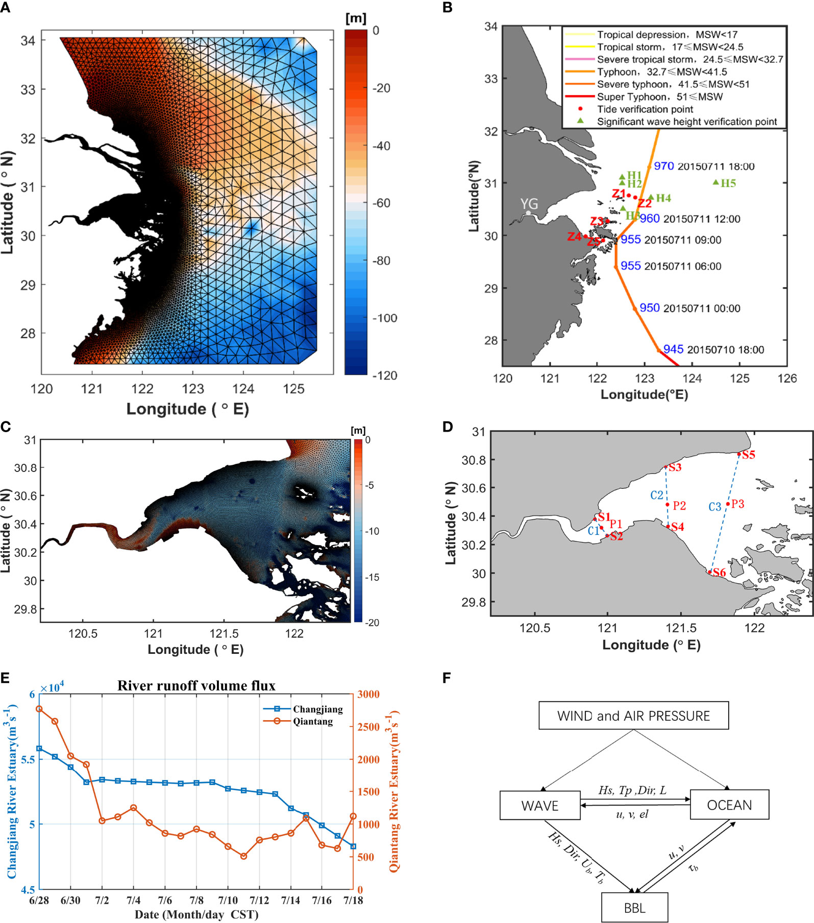
Figure 1 (A, C) Map of Hangzhou Bay and its adjacent seas; grids of the model domain; (B) Typhoon Chan-hom; (D) Distribution of section and feature points. (E) River runoff volume flux (F) Schematic of the coupling between FVCOM circulation model (OCEAN) and FVCOM-SWAVE with inclusion of the wave-current bottom boundary layer model.

2.1.2 Wind Field Re-Construction Model

Pressure and wind field models are essential for accurate storm surge predictions. Parameterized wind field models are widely accepted by oceanographers owing to their high efficiency in calculation (Zhong, 2019). In classic atmospheric models, the wind field comprises a rotating and moving wind field. The former is due to the balance of the pressure gradient, Coriolis, and centrifugal forces, and friction, whereas the latter is mainly related to the movement of the cyclone center (Pan et al., 2016).

The maximum wind speed radius (Table 1), R_max, is the distance between the typhoon center and the maximum wind speed. This is the most important parameter in typhoon models (Chang et al., 2015). The method of Graham and Nunn (1959) (GN59) is a commonly used empirical formula for calculating the maximum wind speed radius in the early stage of typhoon research. Based on a large amount of field data, Knaff et al. (2018) applied the empirical formula of R_max to the western Pacific Ocean, Eastern Pacific Ocean, and Western Atlantic Ocean. Li (2007) studied the correlation between typhoon parameters in the southeast coastal areas of China using the typical correlation analysis method and believed that there was a high correlation between R_max and the central pressure difference. Jiang et al. (2008) proposed an empirical formula for R_max in the form of a power function. This formula is applicable to the northwest Pacific Ocean based on a previous statistical empirical formula and the measured pressure data of the typhoon center.

TABLE 1

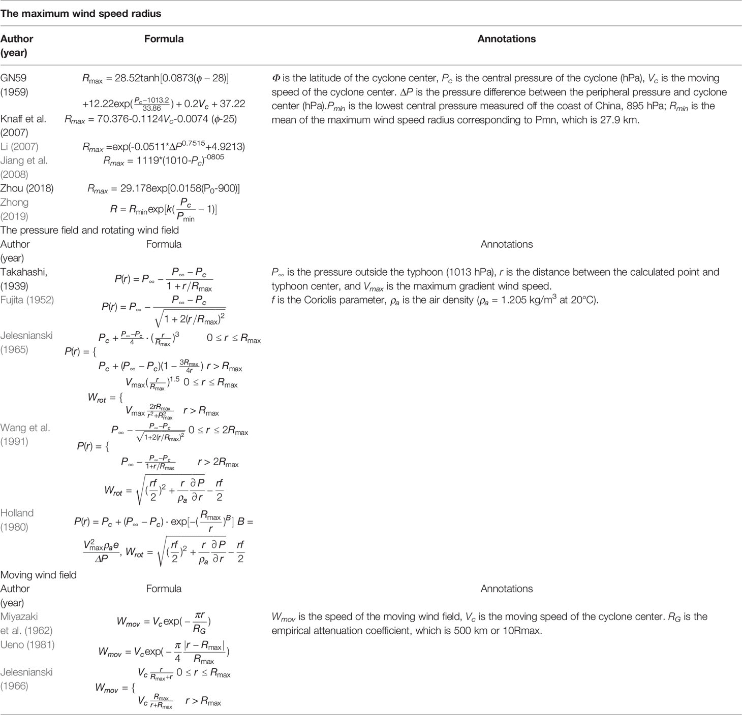
Table 1 Related research on the wind field re-construction.

Typhoon Chan-hom was used as an example to verify the accuracy of the above methods for R_max. The temporal variation in R_maxv, calculated using the above equations, is shown in Figure 2A. The data of geophysical locations, pressure, and moving speed of the typhoon center were obtained from tcdata.typhoon.org.cn (Ying et al., 2014; Lu et al., 2021). According to Zhang (2015), the stronger the typhoon, the smaller the R_max value. R_max calculated according to the method of Knaff (2007), Knaff et al. (2018) has only small temporal variations. The R_max calculated by the GN59 method (Graham and Nunn, 1959) was small, with a smaller R_max occurring when the typhoon was first generated (< 30 h) than that at the peak of the typhoon (75–90 h). These characteristics are not consistent with the physical law of typhoons, indicating that the methods of Graham and Nunn (1959) and Knaff (2007), Knaff et al. (2018) were not suitable for this study.

FIGURE 2

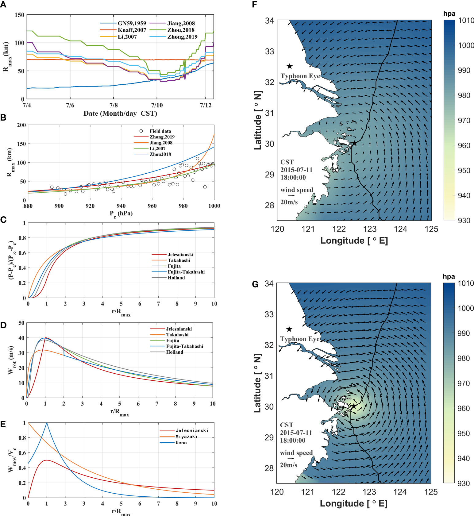
Figure 2 (A) Temporal variation of the maximum wind-speed radius R_max calculated through different empirical formulas. (B)Verification of maximum wind-speed radius R_max calculated by different empirical formulas. (C) Comparison of pressure fields in different models. (D) Contrast of rotating wind field in different models. (E) Comparison of moving wind field in different models. (F) ECMWF wind field at 18:00 on July 11, 2015 (CST, which is China Standard Time). (G)Reconstructed wind field at 18:00 on July 11, 2015 (CST).

To compare the accuracy of the R_max methods, we used typhoon data from the west Pacific in 2013–2015, which were published by the Joint Typhoon Warning Center (JTWC), to perform validations (Figure 2B). The R_max values calculated by Zhou (2018) were relatively large. The R_max calculated by Jiang et al. (2008) model exhibited the best performance when the center pressures were low. However, when the typhoon intensity decayed, the pressure differences decreased, and the deviation of R_max calculated using the method of Jiang et al. (2008) increased quickly. R_max calculated by the methods of Li (2007) (SS=0.737) and Zhong (2019) (SS=0.682) showed better performance. As R_max calculated according to the method of Li (2007) has a higher SS value, we used this method to calculate R_max in this study.

Compared with the moving wind field, the rotating wind field contributed more to the total wind field. It is important to choose a suitable pressure field model for the calculation of the rotating wind field (Table 1). At present, the commonly used air pressure wind field models in China include the Takahashi (Takahashi, 1939), Fujita (Fujita, 1952), Jelesnianski (1966; Jelesnianski, 1965), Fujida–Takahashi (Wang et al., 1991), and Holland models (Holland, 1980).

The Jelesnianski pressure model was proposed by Jelesnianski (1965), and is the pressure field model used by the sea, lake, and overland surges from hurricanes (SLASH). Introducing vorticity theory, Jelesnianski (1965) proposed and improved an empirical formula for the wind field. Through many comparative analyses, Wang et al. (1991) used the Fujita formula (Fujita, 1952) to calculate the distribution of atmospheric pressure in the areas within the distance of 2R_max, and used the Takahashi formula (Takahashi, 1939) to reflect the change of atmospheric pressure in the areas exceed the distance of 2R_max. When air particles move in the atmosphere, the gradient wind formula can be obtained by solving the momentum equation and considering the balance of the pressure gradient force, Coriolis force, and centrifugal force and ignoring the sea surface roughness. Holland (1980) introduced the shape coefficient B and proposed a pressure field model with more general applicability.

The above pressure field model was dimensionless, as shown in Figure 2C, where the shape coefficient B=1.2 was taken from the Holland model. Within the maximum wind speed radius R_max, the growth rate of the Takahashi model was steep and the calculated value was high. The Jelesnianski model had a relatively stable growth rate. The simulation results of the Fujita and Holland models are relatively reasonable. Outside R_max, with an increase in the distance from the typhoon center, the pressure values of all models gradually increased, with a gradually decreasing changing rate, and finally stabilized at P_∞. The Holland model had a relatively large growth rate outside R_max, and the calculated value of the external pressure outside 4R_max was the largest among the five models.

Taking the typhoon Chan-hom as an example, the characteristics of the different rotating wind field models were examined. The Jelesnianski model simulates low wind speeds within R_max, and relatively fast attenuation outside R_max. The maximum wind speed calculated by the Takahashi model was smaller than those of the other models. The representative wind field distribution of the Takahashi model increased with increasing distance from the typhoon center. The maximum wind speed of the Fujita model was closest to reality. The Fujida-Takahashi model absorbs the advantages of both the Takahashi and Fujida models, but the calculated wind speed changes at 2R_max. The wind speed of the Holland model near the typhoon center was smaller than that of the Fujita–Takahashi model, and the Holland wind field outside 2R_max was the largest among the five models.

If the reconstructed wind field contains only the rotating wind field (Figure 2D), then the wind field usually has a spatially symmetric distribution. In the wind field in the northern hemisphere, owing to the movement of typhoons, the rotating wind on the right-hand side and the moving wind superimpose on each other, while canceling each other on the left-hand side. Therefore, the typhoon wind field had a spatially asymmetric distribution. Commonly used models for the calculation of moving wind fields (Table 1) are the Jelesnianski model (Jelesnianski, 1966), Miyazaki model (Miyazaki et al., 1962), and Takeo Ueno model (Ueno, 1981). The moving wind field calculated by the Miyazaki Masawei model (1962) was affected by the empirical attenuation coefficient, and the wind speed decreased with the distance from the typhoon center. The Ueno model (1981) used the maximum wind speed radius to calculate the moving wind field of typhoons.

The moving wind field model above is dimensionless, as shown in Figure 2E. Both the Jelesnianski and Ueno models obtained the maximum wind speed at the maximum wind radius. In the Jelesnianski moving wind field model, the wind speed at the center of the typhoon was zero, R_max reached 0.5V_c, and then the wind speed decreased slowly. In Ueno’s model, the central moving wind speed is approximately 0.456V_c and reaches the maximum value V_c at R_max. Then the wind speed decreases rapidly, and the shifting wind speed was less than 0.1V_c at about 4R_max. The maximum moving wind speed V_c calculated using the Miyazaki model was taken at the center of the typhoon, and the moving wind speed gradually decreased with increasing distance from the typhoon center. The calculated value of V_c using the Miyazaki model at about 5.6R_max was weaker than that calculated using the Jelesnianski model.

In the Jelesnianski moving wind field model, the wind speed at the center of the typhoon was zero, R_max reached 0.5V_c, and then the wind speed decreased slowly. In Ueno’s model, the central moving speed was approximately 0.456 V_c and reached the maximum value V_c at R_max. Then the wind speed decreased rapidly, and the shifting wind speed was less than 0.1 V_c at about 4R_max. The maximum transit wind speed V_c of the Miyazaki Showei model was measured at the center of the typhoon, and the transit wind speed gradually decreased with increasing distance. The calculated value using the Miyazaki model at about 5.6R_max was weaker than that calculated by the Jelesnianski model.

To obtain a more accurate wind field, this study combined the rotation of the wind field, the enhancement, and the NCEP wind field (rda.ucar.edu/datasets/ds084.1). The wind field near the typhoon center mainly depended on the calculated values of the model, whereas the NCEP wind field was applied to a large ocean area. The calculation formula is as follows (Wei et al., 2019):

$\begin{array}{ll}\{\begin{array}{c}{W}_x=\left(1-E\right)\left[W_{mov\_x}-C_1{W}_{rot}\text{sin}\left(\theta +{\beta }_{in}\right)\right]+E{W}_{NCEP\_x}\\ W_y=\left(1-E\right)\left[W_{mov\_y}+C_1{W}_{rot}\text{cos}\left(\theta +{\beta }_{in}\right)\right]+E{W}_{NCEP\_y}\end{array}& (11)\end{array}$

$\begin{array}{ll}E=\frac{C_2^4}{1+C_2^4}& (12)\end{array}$

$\begin{array}{ll}{C}_2=\frac{r}{n{R}_{\max }}& (13)\end{array}$

Where, W_{mov_x} and W_{mov_y} are the x and y components of the moving wind field, and W_{NCEP_x} and W_{NCEP_y} are the x and y components of the NCEP wind field, respectively. θ represents the angle between the line connecting the calculation point with the typhoon center and the east (counter-clockwise). β_in is the inflow angle, representing the deflection angle of the gradient wind vector across the isobars, which is approximately 20° (Wang et al., 1991); and C₁ is the correction coefficient. According to the theory of the atmospheric boundary layer, it is 0.71 (Wei et al., 2017). n = 9 is a constant.

We selected Shipu (121.95°, 29.20°N, 127 m), Dinghai (122.12°, 30.03°, 37 m), Baoshan (121.47°, 31.40°, 4 m), and Qidong (121.60, 32.07°, 10 m) as the field stations to illustrate the reconstructed wind data. The measured wind field data at 10 m was compared with that calculated by different structural wind field models during the influence of typhoon Chan-hom. The data was obtained from the Real-time Database of Atmospheric Environment (envf.ust.hk/dataview) of the Institute of Environmental Science, Hong Kong University of Science and Technology. Near the sea surface, the vertical profile of the wind speed was close to the logarithmic law. The vertical profile of the wind speed was close to the power law from 100 m above the sea surface to the top of the friction layer:

$\begin{array}{ll}\{\begin{array}{cc}\frac{W_{z2}}{W_{z1}}=\frac{\text{lg}{z}_2-\text{lg}{z}_0}{\text{lg}{z}_1-\text{lg}{z}_0}& z\le 100m\\ \frac{W_{z2}}{W_{z1}}={\left(\frac{z_2}{z_1}\right)}^p& z\ge 100m\end{array}& (14)\end{array}$

Where, W_z1 and W_z2 are the wind speeds at altitudes z₁ and z₂, respectively; z₀ is the surface roughness, 0.03 m on the ground and 0.003m on the sea; and P is the empirical coefficient, taking 0.14.

The SS (skill scores) for the different wind models are listed in Table 2. The definition and calculation method of SS are shown in Eq. 17. The rotating wind data dominated the characteristics of the wind field, whereas the moving wind data only slightly adjusted the spatial and temporal distributions of the wind field. The rotating wind data calculated using the Jelesnianski model matched the moving wind data. The rotating wind data calculated using the Fujita-Takahashi model matched the moving wind data of Ueno better. The center wind speed calculated by the Holland method was smaller than that of the field data. The moving wind data calculated using the Miyazaki model enhances the center wind speed calculated using the Holland model. Hence, during typhoon Chan-hom, the Holland-Miyazaki model performed better and was used to reconstruct the wind field data in this study. Wind data reconstructed using the Holland-Miyazaki model are shown in Figures 2F, G.

TABLE 2

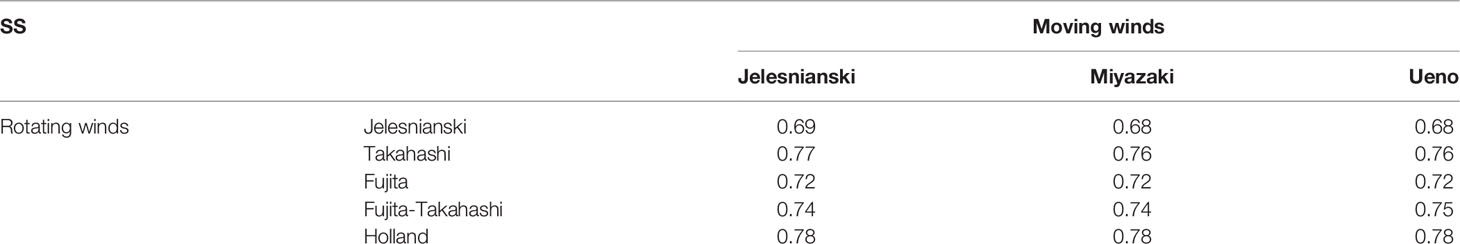
Table 2 SS values of different wind models.

2.2 Model Configurations

2.2.1 Super Typhoon Chan-hom

The super typhoon Chan-hom (International Code: 1509, Joint Typhoon Warning Center: 09 W) was the ninth storm of the 2015 Pacific typhoon season (Figure 1B). At 12:00 on June 30, 2015 (CST, which is China Standard Time), Chan-hom developed over the northwest Pacific Ocean and then moved to the northwest, becoming stronger and reaching super-typhoon level. Chan-hom peaked on July 10 and then entered the East China Sea. At 09:00 on the 11th day, Chan-hom downgraded to a strong typhoon level and landed on the coast of the East China Sea. After landing, Chan-hom moved northward and eastward, and gradually lost its strength.

2.2.2 Model Domain and Configurations

The model domain ranges from 120°E in the west, 125.5°E in the east, 27.5°N in the south, and 34°N in the north, covering the entire Hangzhou Bay, Changjiang River Estuary, and the Zhoushan Islands. To improve computational efficiency and accuracy, the resolution of the model grid was set to 30 km at the open boundary of the ocean. Inside the bay, the resolution of the grid in the coastal area was refined to 200 m and 100 m because of the complex shoreline and island structure (Figures 1A, C).

Shoreline data was obtained from high-precision data provided by the National Geophysical Data Center (NGDC) (https://www.ngdc.noaa.gov/mgg/shorelines/gshhs.html). Bathymetric data was obtained from ETOP1, a global model developed by the National Geophysical Data Center (NGDC). Open-boundary tide data was derived from the global ocean tide prediction model TPXO developed by Oregon State University. The Yangtze River discharge data were obtained from the Datong station of the water level management system (http://yu-zhu.vicp.net/), and sediment discharge data were obtained from the Yangtze River Sediment Bulletin. The flow data of the Qiantang River were obtained from the flow data of the Fuchun River hydrology station (Runoff temperature constant 20°, salinity constant 0‰). Wind and pressure field data under calm weather conditions are derived from reanalysis data provided by the ECMWF (http://apps.ecmwf.int/datasets/data/interim-full-daily/levtype=sfc/). Wind speed data at 10 m above the sea surface was selected as wind forcing data, and sea surface pressure was selected for the air pressure data. The temporal resolution of the two datasets was 6 h and the spatial resolution was 0.125 degree. In addition to the ECMWF data, the wind field and pressure field data during typhoons also included the latitude and longitude, the minimum pressure, and the movement speed of the typhoon center from tcdata.typhoon.org.cn.

2.3 Numerical Tests

Eight numerical experiments were designed based on the tide-wave coupling numerical model (Table 3). Case 0 is the control run. Case 1 removes the wind field based on the control condition (Case 0). Case 2 removes the influence of air pressure based on Case 0. Case 3 removes the wave action based on Case 0. Based on the controlling experimental Case 0, Case 4 removes the effects of wind field, air pressure, and waves. There is a nonlinear relationship between the increase in wind stress and astronomical tidal level. To explore the relationship between winds and astronomical tidal level, a numerical simulation (Case 5) was designed. In Case 5, only wind forcing was considered and tidal forcing was removed. To explore the relationship between wave-induced surges and astronomical tide levels, numerical simulation Case 6 was designed. In Case 6, only wave was considered and tide was removed. Numerical simulation Case 7 was set up to further investigate the nonlinear effect of the wind field and astronomical tide. Case 7 considered wind, wave and air pressure, but ignored tidal forcing.

TABLE 3

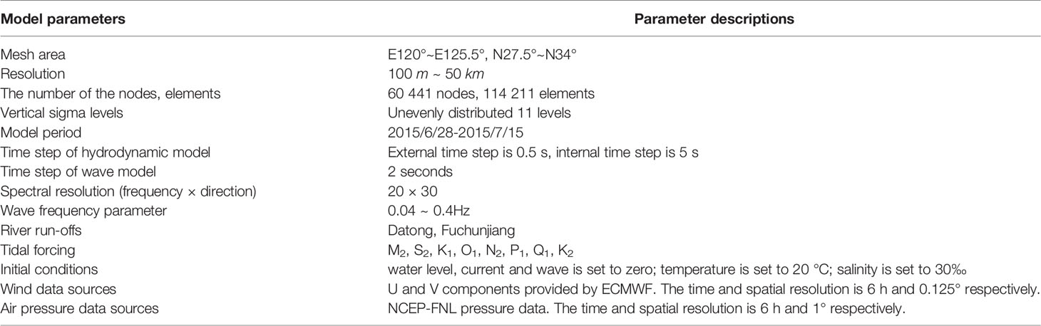
Table 3 Model configuration.

3 Model Verification

3.1 Field Data

The distribution of field stations is shown in Figure 1B. The measured data were obtained from the Shanghai Meteorological Administration Numerical Prediction Innovation Center and Zhejiang Ocean Monitoring and Prediction Center. The measured tidal level data are at five stations, Z1, Z2, Z3, Z4, and Z5, as shown in Figure 1B. The tidal flow verification only includes H3/W4 in Figure 1B. The wave measured data were obtained from five stations, H1, H2, H3, H4, and H5, from July 1 to July 15, 2015 (CST, Figure 1B).

Root mean squared error (RMSE), correlation coefficient (CC) and skill scores (SS) were used to evaluate the reliability and accuracy of the model (Murphy, 1992):

$\begin{array}{ll}\text{RMSE=}{\left[\frac{1}{\text{N}}{\displaystyle \sum _{i=1}^N{\left(M_i-O_i\right)}^2}\right]}^{\mathrm{1 / 2}}& (15)\end{array}$

$\begin{array}{ll}CC=\frac{1}{N}{\displaystyle \sum _{i=1}^N\frac{\left(m_i-\overline{m}\right)\left(O_i-\overline{O}\right)}{S_m{S}_o}}& (16)\end{array}$

$\begin{array}{ll}SS=1-\frac{{\displaystyle \sum _{i=1}^N{\left(m_i-O_i\right)}^2}}{{\displaystyle \sum _{i=1}^N{\left(O_i-\overline{O}\right)}^2}}& (17)\end{array}$

where m_i and O_i are the model simulation and measured data, respectively.$\overline{m}$ and $\overline{O}$ are the averages of the simulated and measured values, respectively. S_m and S_o are the standard deviations of the simulated and measured values. The closer the correlation coefficient (CC) is to one, the greater the correlation between the simulated and measured values. When the skill scores (SS) is greater than 0.2, the model has some reliability. When the skill scores (SS) is greater than 0.5, the model is highly reliable.

3.2 Model Validation

Tidal levels at the five sites Z1, Z2, Z3, Z4, and Z5 (red dot in Figure 1B). The data period was from July 1 to July 15, 2015 (CST). The CC and SS of the statistical error between the simulated and observed tidal levels at each station is shown in Table 4. The CC and SS of tidal levels at each station is between 0.96 and 0.98 (Table 4). The model simulates the changes better in the tidal level during typhoons (Figure 3A).

TABLE 4

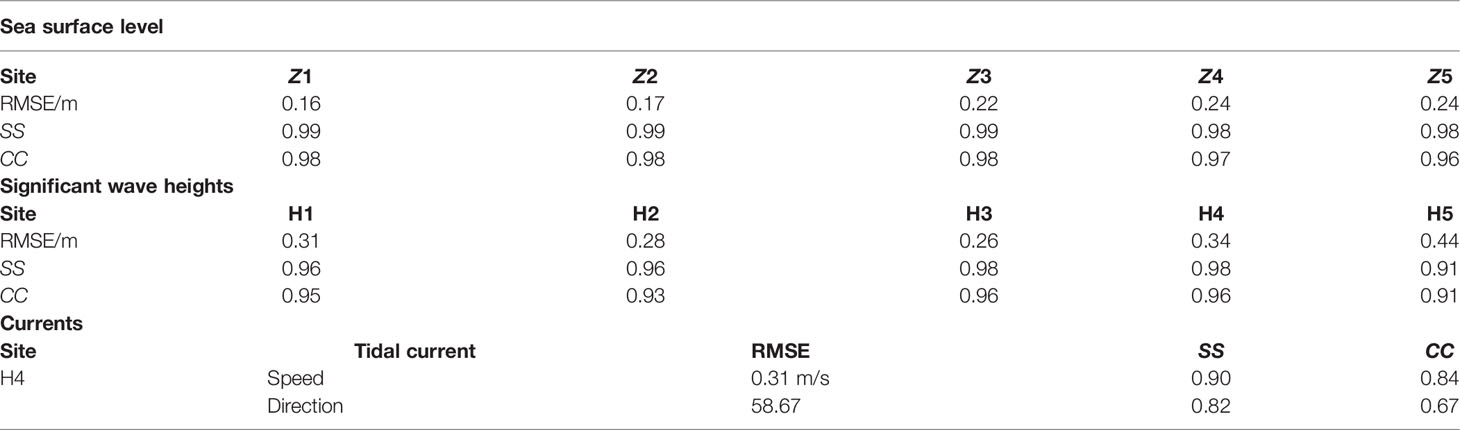
Table 4 Statistics of tide level verification during the typhoon.

FIGURE 3

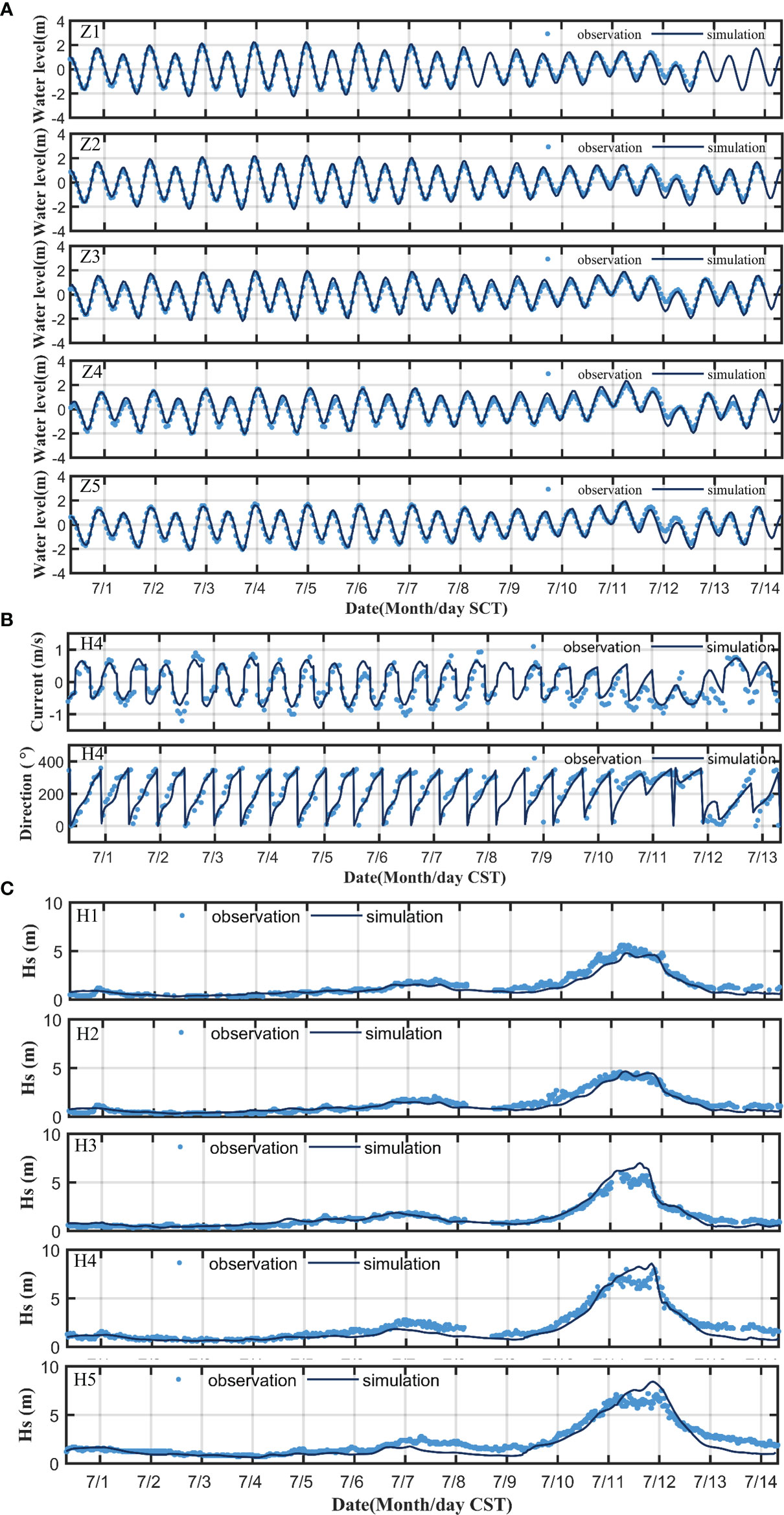
Figure 3 (A) Comparison of simulated and observed water levels at Z1 to Z5 stations. (B) Current speed and current direction at H4 station. (C) Comparison of simulated and observed significant wave height.

The tidal flow verification data of the H4 station are from July 1 to July 15, 2015 (CST, Figure 1B). The flow speed validation SS is 0.88 and the CC is 0.81. The flow direction validation SS is 0.82 and the CC is 0.67 (Table 4). The tidal current verification is within an acceptable accuracy range (Figure 3B). More information on model validation was provided by Ye (2019) and Ren (2022).

Significant wave height data were obtained from stations H1 to H5 (green points in Figure 1B) at the verification site. The data period was from July 1 to July 15, 2015 (CST). The SS for the significant wave height at each site was higher than 0.95, and the minimum CC was 0.93 (Table 4). The simulated wave height was in good agreement with the measured value (Figure 3C). The model can accurately simulate the processes of wave generation and extinction during typhoons.

4 Results

4.1 Tides and Storm Surges

Three sections (C1, C2, and C3) and six points (S1, S2, S3, S4, S5, and S6) were used to illustrate the characteristics of the tides and surges in the bay. The water depth of the six feature points is 9.0 m, 14.7 m, 6.5 m, 12.9 m, 8.0 m, and 11.0 m, respectively. The surges during the storm tides is represented by the differences between the sea surface level in Case 0 (the control run, Table 5) and the sea surface level in calm weather (Case 4, Table 5).

TABLE 5

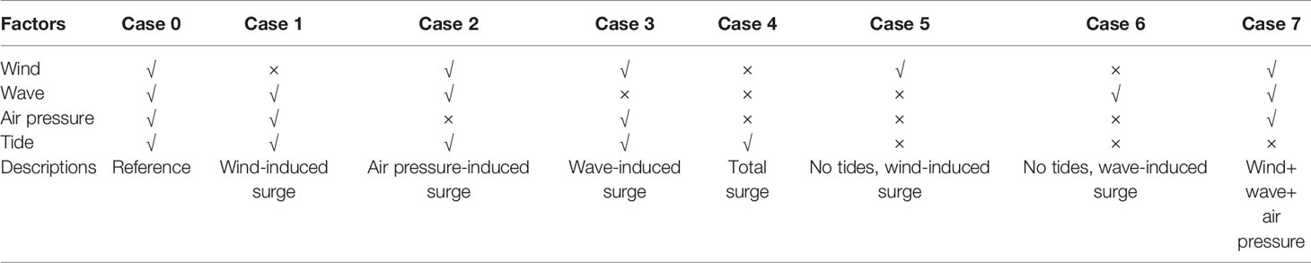
Table 5 Numerical tests.

Typhoon Chan-hom passed through Hangzhou Bay and its nearby areas from July 10 - 11, 2015 (CST, Figures 4A, B). As the typhoon gradually approached, the sea surface level at the mouth of the bay was initially affected. It began to increase, and the maximum sea surface level at section C3 at the bay mouth reached 2.5 m. At 09:00 on July 11, the sea surface level at section C1 at the bay head reached 4.0 m, and then the maximum sea surface level areas continued to advance upstream, and finally reached a peak of 5.0 m at Yanguan. Similarly, the area of peak increase in sea surface level also began to advance from the bay mouth to the bay head. The maximum sea surface level at section C3 at the mouth of the bay was about 1.2 m, and the maximum sea surface level at section C2 at the middle of the bay was 1.5 m. Finally, at 09:00 on July 11, the maximum increase value of sea surface level (3.0 m) was reached at the head of the bay, and the variation trend of the two was basically the same.

FIGURE 4

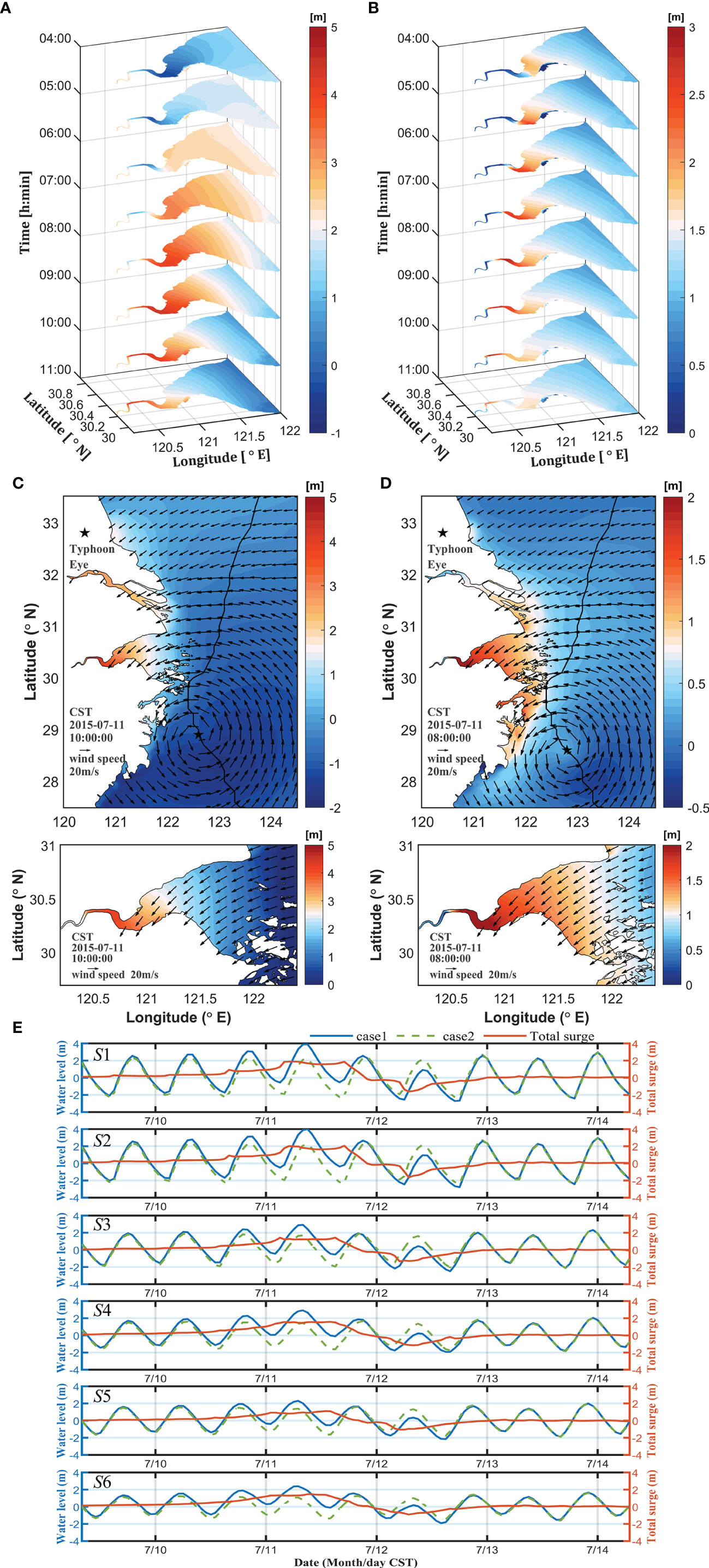
Figure 4 Distribution of total water level and total surge during the typhoon from 04:00 to 11:00, July 11: (A) Total water level and (B) Total surge. (C) Sea surface level at 02:00, July 11. (D) Surges at 00:00 on July 11. (E) Sea surface level and total surge time series at each feature point (July 9-14). The green dashed line is the water level with only tidal forcing, blue solid line is the water level during the typhoon, and the orange line is the surge.

In the bay mouth, the surge always remained small, the bay mouth was relatively wide, and the backwater effect caused by winds and waves was small. The surge increases earlier than the sea surface level, and the maximum surge moment occurs earlier than the moment of the high slack water level.

The maximum sea surface level and surge occurred when Hangzhou Bay was at the radius of the maximum wind speed (Figures 4C, D). The wind speed in the bay was relatively uniform. Due to the influence of the funnel-shaped topography of the bay, the maximum water level and maximum water surge both occur at the narrow bay head and the maximum water level is up to 5.0 m in the upstream Yanguan station (YG in Figure 1B). The surge at the bay head was generally more than 2.0 m, and the surge at Yanguan was the largest, up to 3.0 m.

In counter-clockwise cyclones, sea surface water was driven by wind from the northern areas to the southern area and blocked by the southern coastlines. Larger sea surface level and surge occurred near the southern bank. Spatially asymmetric distributions of the sea surface level and surge occurred owing to the impacts of typhoons and geomorphology. The sea surface level in the bay was approximately 1 m and 0.5 m higher than in the open ocean and bay mouth, respectively.

The surge is mainly related to the wind field. Figure 4E shows the time series of the total water level and surge at each feature point. The maximum water level at the six feature points is 4.03 m, 4.06 m, 2.93 m, 2.96 m, 2.21 m, and 2.44 m, respectively (Figure 4E). In all three sections, the water level on the southern bank (points S2, S4, S6) is lower than that on the northern bank (points S1, S3, S5). The maximum water level of the six feature points occurred in high slack water, and the difference between them was small.

The maximum surge of the six feature points is 1.95 m, 2.04 m, 1.67 m, 1.74 m 1.12 m and 1.50 m, respectively. The peak surge at the bay mouth was less than that at the head of the bay, and there was no difference between the peak surge in the southern and northern areas. The maximum surge time of the six feature points was gradually delayed from the mouth to the bay head. With the movement of typhoons, the peak surge rapidly advances into the bay. With the advancement of typhoons, the extreme value of the surge rapidly advances into the bay. At extreme water levels, the tide level dominates, and the tide levels at all points in the bay are relatively synchronized. Therefore, the maximum water level at each point is similar, and the extreme water level advances slowly into the bay.

Under the influence of typhoon Chan-hom, the surge in Hangzhou Bay is mainly of standard and mixed types. The surge curve at S1 and S2 has three obvious stages: forerunner, storm surge, and residual vibration. The standard type occurred at four other stations. Owing to the small peak value of the surge, the surge curve was relatively mild, generally in the form of tidal waves. There are small fluctuations at some moments, so they are a mixture of standard and fluctuation types.

4.2 Currents

According to the time series in Figure 3B, the main period for the storm to affect the hydrodynamic environment in the bay was from 02:00 to 13:00 on July 11, 2015 (CST). Therefore, four moments were selected during the tidal period to illustrate the currents during the typhoon: ebb slack (02:00), flood peak (05:00), flood slack (08:00), and ebb peak (11:00). Surface currents are mostly controlled by the typhoon winds. The flow field in the typhoon center is consistent with the typhoon wind field and circulated counterclockwise around the typhoon center. The flow field had one one-hour time lag compared with the wind field. The velocities of the flow field on the left and right sides of the typhoon center were large, whereas the velocities on the upper and lower sides were relatively small. This is because the wind field to the right of the typhoon center moves in the same direction as the typhoon, and the two are superimposed onto each other to create a higher velocity. The left side of the typhoon was near the shoreline, and water movement was impacted by the shorelines. The water channel was relatively narrow; therefore, the velocity in this area was high.

The typhoon was far from the bay at the ebb slack (Figure 5A). The coastal area of the southern East China Sea was affected by the typhoon, and the coastal current extended from northeast to southwest, with a velocity of up to 1.5 m/s. There are still ebbing tides in the inner part of the bay, but the estuary and open sea started to flood. The upstream ebbing currents meet open-sea flooding currents, forming a southward tidal current with a low velocity of approximately 0.2 m/s. At the flood peak (Figure 5B), the offshore tidal current moved from the southeast to northwest directions, with a small velocity of approximately 0.7 m/s. When the tidal current enters the bay, the velocity is large in the narrow tidal channel and is relatively uniform inside the bay, ranging from 1.0 m/s to 1.5 m/s. At the flood slack (Figure 5C), except for the area near the typhoon center where the velocity was high, the velocity in other sea areas was below 0.5 m/s. The offshore flow direction is basically northward, whereas the nearshore current turns northwest. Ebb tides are still dominant in Hangzhou Bay. At the peak ebb tide (Figure 5D), coastal waters were strongly affected by the typhoon, with a maximum velocity of up to 2 m/s. The water moved southward along the coast with larger offshore currents. The water in the bay ebbed into the East China Sea with a velocity of 1.5 m/s in the narrow tidal channels at the bay mouth owing to the constraints of island topography. The flow velocity inside the bay was approximately 1 m/s. The flow directions were restricted by topography.

FIGURE 5

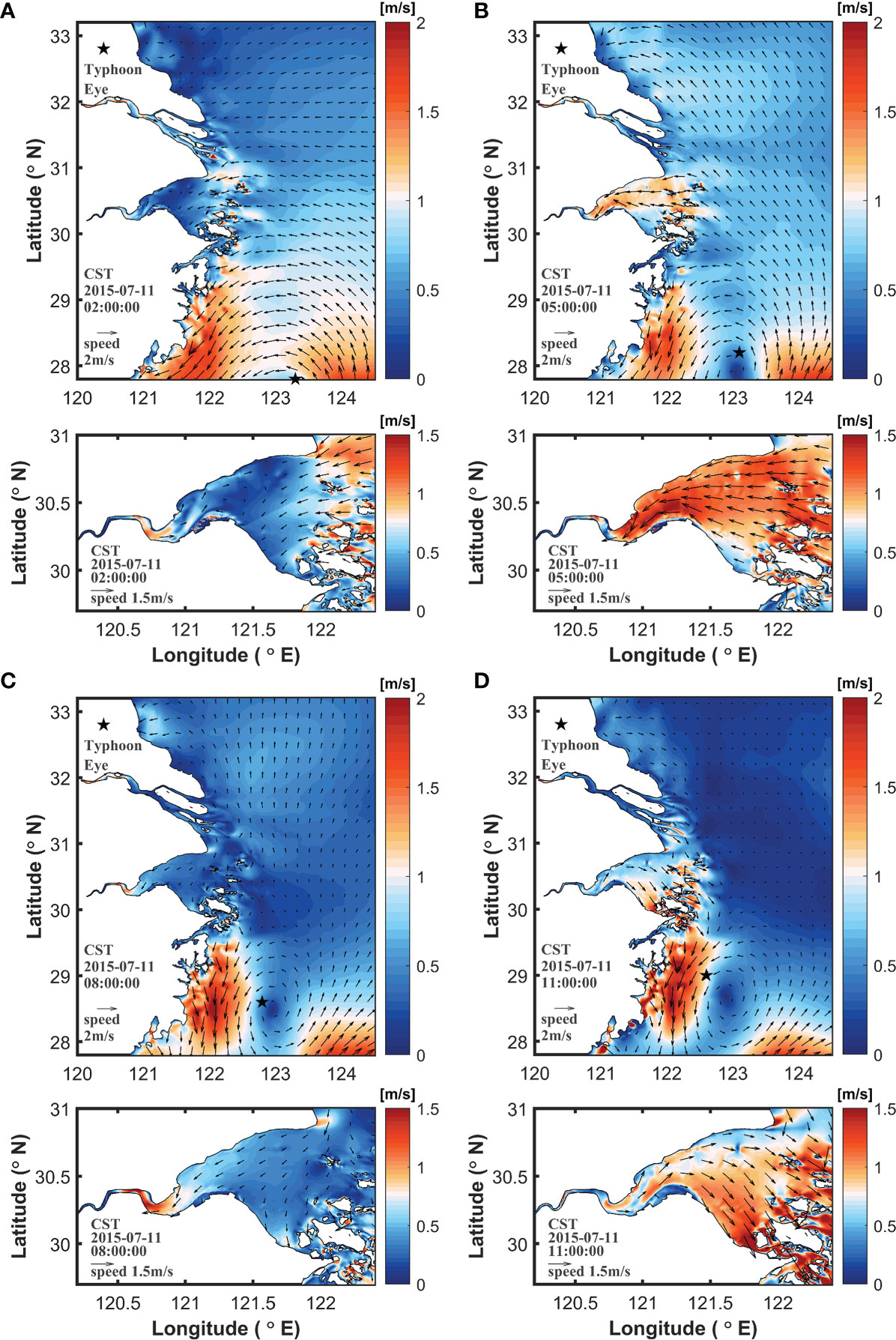
Figure 5 Surface flow field at (A) 02:00, (B) 05:00, (C) 08:00 and (D) 11:00 on July 11, 2015 (CST).

4.3 Waves

The distribution of the significant wave heights of typhoon waves is closely related to the distribution of typhoon wind fields (Figure 6). Inside the bay, the significant wave height (Hs) was lower than that in the open sea. The significant wave height was higher near the southern bank and near the bay mouth during the typhoon (Figures 6A, B). The peak value of the significant wave height occurred near the mouth of HZB at 8:00 on July 11, 2015 (CST). With the approach of the typhoon wind field, the wave heights in the bay gradually increased, and the maximum wave height was 3.5 m in the bay mouth. Inside the bay, the wave height is mostly below 1.0 m. With the approach of the typhoon, the contour line of the Hs=2 m gradually expanded and extended into the bay, and the contour line of Hs=3 m was always concentrated in the central area of the bay mouth.

FIGURE 6

Figure 6 Significant wave heights inside the bay at: (A) 04:00 to 11:00 (B) 12:00 to 19:00 on July 11. Significant wave heights at (C) 05:00, (D) 11:00, (E) 17:00 and (F) 23:00 on July 11.

In the open sea, the significant wave heights were distributed in an elliptical shape, and the wave heights were the largest at the center of the ellipse and decreased towards the periphery. The wave height in the sea area to the right of the typhoon center (along the direction of typhoon movement) was generally higher than that of the sea area to the left of the typhoon center (Figures 6C–F). The direction of the wind speed on the right side of the typhoon center was the same as the typhoon moving direction, and the wind speed after superposition of the two was greater than that on the left side of the typhoon center. Therefore, in the open sea, the development of wind waves on the right side of the typhoon center was better than that on the left side. The wave height was greater than that on the left side of the typhoon center. The distribution of the significant wave height was also restricted by the terrain. Because the center of the typhoon is close to the shoreline, the typhoon waves are easily blocked by the shoreline during the growth of the typhoon waves along the direction of the wind speed (Figure 6D), so that the water body accumulates, and the significant wave height increases. Therefore, at this moment, large significant wave heights occurred on the right and upper sides of the typhoon center. Because the center of the typhoon is far from the coastline and the nearby sea area is open, a larger wave height occurs only on the right side of the typhoon center (Figure 6F).

4.4 Wind-Induced Surge

During the typhoon (09:00-13:00 on July 11), the surges caused by wind stress in the inner area of Hangzhou Bay (S5 and S6) reached their maximum values of 1.27 m and 0.99 m, respectively (Table 6). At 14:00 and 15:00 on July 11, the surge reached the central area of the bay (S3). Finally, at 17:00 on July 11, the storm surge induced by wind stress in the bay head reached a maximum value. The peak surge caused by wind stress at each station were approximately 96%, 96%, 92%, 93%, 86%, and 90% of the total storm surge, respectively. In general, there are small differences in the magnitudes of storm surges between the northern and southern banks. The peak value of storm surge increased from the mouth to the head of the bay. This is because the reduction in the width and water depth from the mouth to the head of the bay reduces the tidal prism and amplifies the shallow water effect.

TABLE 6

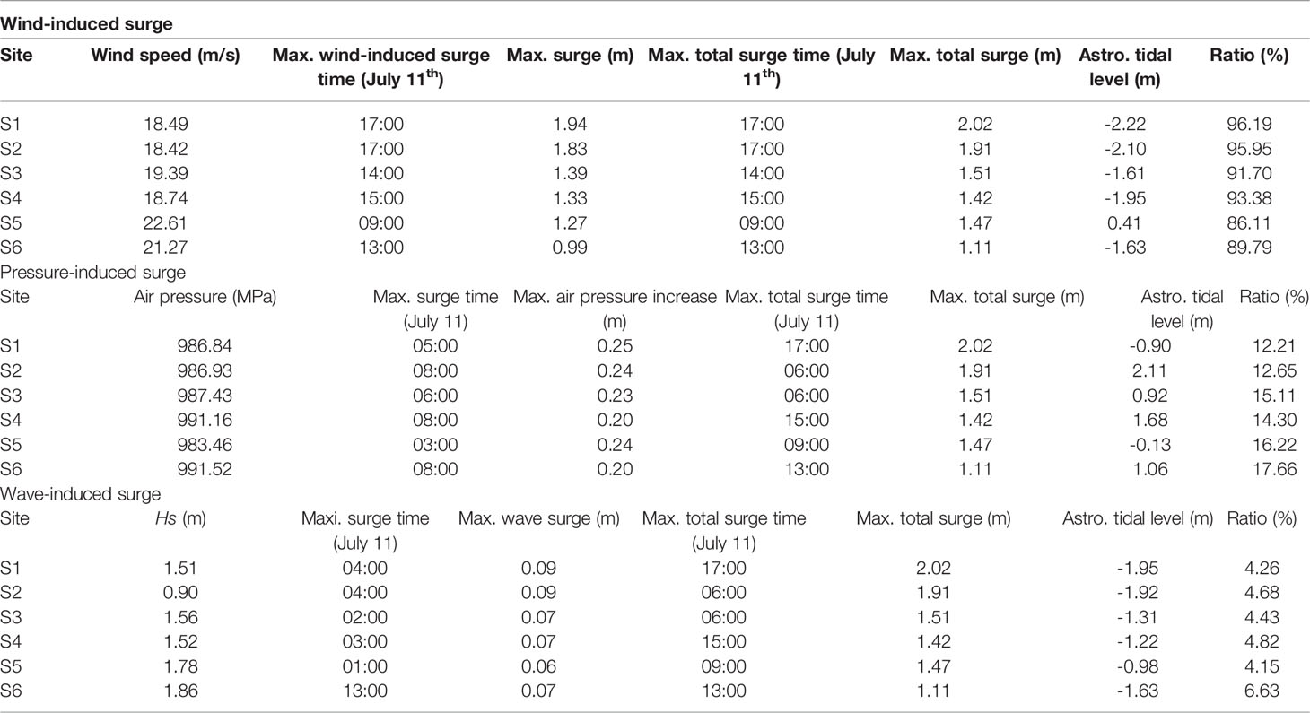
Table 6 Summary of characteristic values of wind-induced surge, pressure-induced surge and wave-induced surge.

Wind stress is critical for storm surges (Figure 7I). The wind-induced surge time series coincided with the total surge curve, except for divergence during typhoon landing. The total surge was slightly larger than the wind-induced surge during typhoons. The average ratio of the peak values of wind-induced surges at the six feature points was 91%. The peak values of wind stress and surge at the six feature points were consistent with the peak values of the total surge, indicating that wind stress was the main factor leading to storm surges.

FIGURE 7

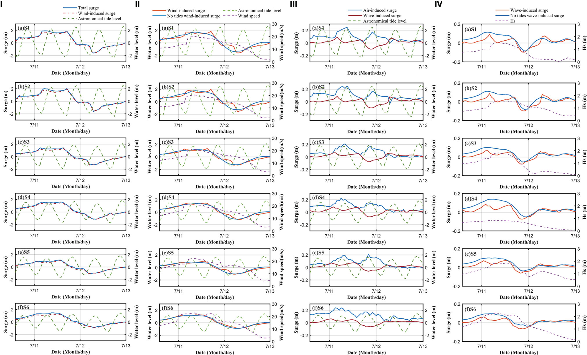
Figure 7 (I) Comparison of wind-induced surge and total surge (July 10-13: green dotted line is astronomical tide level, blue solid line is total surge, red solid line is wind-induced surge). (II) Comparison of wind-induced storm surge with tidal forcing and without tidal forcing (July 10-13). (III) Comparison of pressure-induced, wave-induced and astronomical tide level in July 10-13. (IV) Comparison of wave-induced surge and without tides (July 10-13).

The spatial distribution of wind stress and storm surge at 17:00 on July 11 is illustrated (Figure 8A), when the peak values of wind stress and surge occurred. At this moment, the typhoon center is located on the southeast side of the HZB. A northeasterly wind prevails in the bay, and the wind speed is approximately 20 m/s. The southern part of the typhoon center was dominated by a decrease in water, whereas the northern part was dominated by an increase in water. This pattern was mostly controlled by the wind and local morphology.

FIGURE 8

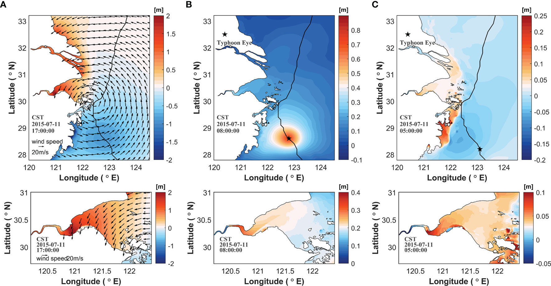
Figure 8 (A) Wind speed and wind-induced surge at 17:00 on July 11. Vectors indicate wind speeds and contours indicate surges. (B) Pressure-induced surge at 00:00 on July 11. (C) Wave-induced surge at 21:00 on July 10.

The peak of wind-induced storm surges always occurs during the low tide period (Figure 7). Case 5 was designed with the tidal level ignored at the open boundary to explore the nonlinear effect between the wind-induced storm surges and astronomical tides. In regions with a large water depth, tidal fluctuation has little influence on the wind-induced surge mechanism. Therefore, at feature points S3-S6, the wind-induced surge in Case 5 was nearly the same as that in control, Case 0. For shallow regions, the water level is closely related to astronomical tides. The vertical distribution of the wind-induced shear on the water body was also affected by the water level. Therefore, when the wind speed is high and changes significantly, the surges in Cases 0 and 5 at stations S1 and S2, which are in shallow water areas, are different. The surge without tidal forcing (Case 5) was relatively gentle compared with the surge with tidal forcing (Case 0). The surge with tidal forcing showed multiple peaks, and peak values occurred at the low slack waters. This is because the depth of low slack waters is shallow, and the wind stress is stronger, leading to a larger storm surge.

The wind-induced surge was controlled by both wind speed and tidal level. During typhoons, the maximum times of stress and storm surges were slightly different. In the absence of tidal forcing, the maximum wind-induced surge occurred at the time of maximum wind speed. Under the influence of tides, the maximum value of the wind-induced surge occurs in low slack waters near the peak wind speed moment.

4.5 Air Pressure-Induced Surge

During the typhoon, the air pressure exhibited clear spatial variations. The air pressure was low in the center of the typhoon and increased in the surrounding areas. By comparing the water levels of Cases 0 and 2 (Table 5), the intensity of the air pressure-induced surge was evaluated (Table 6; Figure 7III).

The pressure-induced storm surge curve was relatively stable with no obvious peak values. The typhoon center was south of the HZB, and the southern bank was first impacted by the low-pressure area of the typhoon center. Therefore, the peak surge moment of each feature point is obviously different: the southern bank is approximately 05:00 on July 11, and the northern bank is 08:00 on July 11. During the typhoon, the pressure change in the HZB was small, so the pressure-induced storm surge was mostly uniform. The increase in water pressure caused by the decrease in air pressure was small, and the peak value of the air pressure-induced surge was relatively small compared to the peak value of the total surge. The proportions of each feature point (S1-S6) were 12%, 13%, 15%, 14%, 16%, 18%, respectively, and the average value 15%. The typhoon passes through the HZB from the outer sea, and the bay mouth is closer to the typhoon center. Therefore, the pressure-induced surges at S5 and S6 near the bay mouth were higher than those at the other four points.

Taking the time of the maximum storm surge at the bay head caused by atmospheric pressure as the reference time (08:00 on July 11), atmospheric-induced surges generally occurred in Hangzhou Bay (Figure 8B). As the pressure was lowest at the center of the typhoon, it increased from the center to the periphery. At this time, the typhoon cyclone center was in the southeast of Hangzhou Bay, so the sea area south of Hangzhou Bay near the typhoon cyclone center had a large increase in atmospheric pressure and a water level of more than 0.3 m. The pressure-induced surge in Hangzhou Bay was largely uniform, approximately 0.2 m. The maximum pressure-induced surge was approximately 0.27 m at the head of the bay.

4.6 Wave-Induced Surge

The water levels of Cases 0 and 3 (Table 5) were compared to evaluate the surge caused by waves in the storm surge (Table 6; Figure 7III). The wave-induced surges were weak (Table 6). The proportions of wave-induced and total storm surges of the six feature points were 4, 5%, 4%, 5%, 4%, and 7%, respectively. The changes in significant wave height during typhoons are caused by wind, therefore, the peak time of the wave-induced storm surge is consistent with the peak time of wind-induced and total surges. The peak value of the wave-induced surge occurred first at the mouth of the bay and then in the middle and head of the bay. This process is consistent with the passage of the maximum wind radius.

The peak moment of the wave-induced surge at the head of the bay was selected as the reference time (21:00 on July 10), and its spatial distribution was illustrated (Figure 8C). The maximum wind speed radius of the typhoon was at the top of the bay, and the wave surge in HZB decreased from the top to the mouth of the bay. The wave-induced surge at the top of the bay was 0.1 - 0.15 m. In the middle and mouth of the bay, the coastline is relatively smooth, and the wave surge was almost the same between the northern and southern banks. The wave-induced surge in the bay was about 0.07 m and 0.04 m at the head and the mouth.

Wave-induced surges peaked in low-slack waters. Case 6 was designed while ignoring the astronomical tides to explore the nonlinear effect between wave-induced surges and astronomical tides (Figure 7IV). The wave-induced surge without tidal forcing (case 6, blue line in Figure 7IV) was consistent with the variation in the significant wave height (dotted purple line in Figure 7IV). The greater the significant wave height, the greater the wave-induced surge. The peak of the wave-induced surge occurred slightly later than that of the significant wave height. In this test, it is assumed that the tide level is always zero and that there is always wave forcing at the boundary, which leads to water imbalance in the model domain, and the wave-induced surge is always positive. In the case of tidal forcing (Case 0), when the significant wave height was small, the wave-induced surge was close to zero. With an increase in the significant wave height during typhoons, the wave-induced surge begins to increase. There are two peaks of wave-induced surges, which all occur in low-slack waters.

5 Discussion

5.1 Tide-Surge Interaction

Hangzhou Bay is funnel-shaped, with strong tides. To study the nonlinear interaction between tides and surges, equations (2) and (3) can be rewritten as follows:

$\begin{array}{ll}\begin{array}{c}\frac{\partial u}{\partial t}+\frac{\partial u^2}{\partial x}+\frac{\partial uv}{\partial y}+\frac{\partial uw}{\partial \sigma D}-fv=-g\left[\frac{\partial \left(\zeta \right)}{\partial x}+\frac{1}{{\rho }_0}\left(\frac{\partial }{\partial x}\left(D{\displaystyle \underset{\sigma }{\overset{0}{\int }}\rho d\sigma }\right)+\sigma \rho \frac{\partial D}{\partial x}\right)\right]\\ -\frac{\partial \left(P_{atm}\right)}{\partial x}+\frac{1}{D^2}\frac{\partial }{\partial \sigma }(K_m\frac{\partial u}{\partial \sigma })+F_u+R_x/D\end{array}& (18)\end{array}$

$\begin{array}{ll}\begin{array}{c}\frac{\partial v}{\partial t}+\frac{\partial uv}{\partial x}+\frac{\partial v^2}{\partial y}+\frac{\partial vw}{\partial \sigma D}+fu=-g\left[\frac{\partial \left(\zeta \right)}{\partial y}+\frac{1}{{\rho }_0}\left(\frac{\partial }{\partial y}\left(D{\displaystyle \underset{\sigma }{\overset{0}{\int }}\rho d\sigma }\right)+\sigma \rho \frac{\partial D}{\partial y}\right)\right]\\ -\frac{\partial \left(P_{atm}\right)}{\partial y}+\frac{1}{D^2}\frac{\partial }{\partial \sigma }(K_m\frac{\partial v}{\partial \sigma })+F_v+R_y/D\end{array}& (19)\end{array}$

The terms on the left side are the local acceleration, advection, and Coriolis force along the estuary. The terms on the right side are the surge, barotropic, baroclinic, air pressure, friction dissipation, horizontal momentum diffusion, and wave radiation stress.

To simplify the discussion, the momentum equation was derived and transformed by ignoring the diffusion term. When only tidal forcing is considered, the equations can be rewritten as

$\begin{array}{ll}\begin{array}{c}\frac{\partial u_T}{\partial t}+\frac{\partial u_T^2}{\partial x}+\frac{\partial u_T{v}_T}{\partial y}+\frac{\partial u_T{w}_T}{\partial \sigma D_T}-fv=-g\left[\frac{\partial \left({\zeta }_T\right)}{\partial x}+\frac{1}{{\rho }_0}\left(\frac{\partial }{\partial x}\left(D_T{\displaystyle \underset{\sigma }{\overset{0}{\int }}\rho d\sigma }\right)+\sigma \rho \frac{\partial D_T}{\partial x}\right)\right]\\ -\frac{\partial \left(P_{atm}\right)}{\partial x}+\frac{1}{D_T^2}\frac{\partial }{\partial \sigma }(K_m^T\frac{\partial u_T}{\partial \sigma })+F_u+R_x/D\end{array}& (20)\end{array}$

$\begin{array}{ll}\begin{array}{c}\frac{\partial v_T}{\partial t}+\frac{\partial u_T{v}_T}{\partial x}+\frac{\partial v_T^2}{\partial y}+\frac{\partial v_T{w}_T}{\partial \sigma D_T}+fu=-g\left[\frac{\partial \left({\zeta }_T\right)}{\partial y}+\frac{1}{{\rho }_0}\left(\frac{\partial }{\partial y}\left(D_T{\displaystyle \underset{\sigma }{\overset{0}{\int }}\rho d\sigma }\right)+\sigma \rho \frac{\partial D_T}{\partial y}\right)\right]\\ -\frac{\partial \left(P_{atm}\right)}{\partial y}+\frac{1}{D_T^2}\frac{\partial }{\partial \sigma }(K_m^T\frac{\partial v_T}{\partial \sigma })+F_v+R_y/D\end{array}& (21)\end{array}$

Considering only winds, air pressure, and waves, the equations can be rewritten as follows:

$\begin{array}{ll}\begin{array}{l}\frac{\partial u_S}{\partial t}+\frac{\partial u_S^2}{\partial x}+\frac{\partial u_S{v}_S}{\partial y}+\frac{\partial u_S{w}_S}{\partial \sigma D_S}-fv=-g\left[\frac{\partial \left({\zeta }_S\right)}{\partial x}+\frac{1}{{\rho }_0}\left(\frac{\partial }{\partial x}\left(D_S{\displaystyle \underset{\sigma }{\overset{0}{\int }}\rho d\sigma }\right)+\sigma \rho \frac{\partial D_S}{\partial x}\right)\right]\\ -\frac{\partial \left(P_{atm}\right)}{\partial x}+\frac{1}{D_S^2}\frac{\partial }{\partial \sigma }(K_m^S\frac{\partial u_S}{\partial \sigma })+F_u+R_x/D\end{array}& (22)\end{array}$

$\begin{array}{ll}\begin{array}{c}\frac{\partial v_S}{\partial t}+\frac{\partial u_S{v}_S}{\partial x}+\frac{\partial v_S^2}{\partial y}+\frac{\partial v_S{w}_S}{\partial \sigma D_S}+fu=-g\left[\frac{\partial \left({\zeta }_S\right)}{\partial y}+\frac{1}{{\rho }_0}\left(\frac{\partial }{\partial y}\left(D_S{\displaystyle \underset{\sigma }{\overset{0}{\int }}\rho d\sigma }\right)+\sigma \rho \frac{\partial D_S}{\partial y}\right)\right]\\ -\frac{\partial \left(P_{atm}\right)}{\partial y}+\frac{1}{D_S^2}\frac{\partial }{\partial \sigma }(K_m^S\frac{\partial v_S}{\partial \sigma })+F_v+R_S/D\end{array}& (23)\end{array}$

Considering tides, wind fields, air pressure, and waves, the equations are as follows:

$\begin{array}{ll}\begin{array}{c}\frac{\partial u_{T+S}}{\partial t}+\frac{\partial u_{T+S}^2}{\partial x}+\frac{\partial u_{T+S}{v}_{T+S}}{\partial y}+\frac{\partial u_{T+S}{w}_{T+S}}{\partial \sigma D_S}-fv=-g\left[\frac{\partial \left({\zeta }_{T+S}\right)}{\partial x}+\frac{1}{{\rho }_0}\left(\frac{\partial }{\partial x}\left(D_{T+S}{\displaystyle \underset{\sigma }{\overset{0}{\int }}\rho d\sigma }\right)+\sigma \rho \frac{\partial D_{T+S}}{\partial x}\right)\right]\\ -\frac{\partial \left(P_{atm}\right)}{\partial x}+\frac{1}{D_{T+S}^2}\frac{\partial }{\partial \sigma }(K_m^{T+S}\frac{\partial u_{T+S}}{\partial \sigma })+F_u+R_x/D\end{array}& (24)\end{array}$

$\begin{array}{ll}\begin{array}{c}\frac{\partial v_{T+S}}{\partial t}+\frac{\partial u_{T+S}{v}_{T+S}}{\partial x}+\frac{\partial v_{T+S}^2}{\partial y}+\frac{\partial v_{T+S}{w}_{T+S}}{\partial \sigma D_{T+S}}+fu=-g\left[\frac{\partial \left({\zeta }_{T+S}\right)}{\partial y}+\frac{1}{{\rho }_0}\left(\frac{\partial }{\partial y}\left(D_{T+S}{\displaystyle \underset{\sigma }{\overset{0}{\int }}\rho d\sigma }\right)+\sigma \rho \frac{\partial D_{T+S}}{\partial y}\right)\right]\\ -\frac{\partial \left(P_{atm}\right)}{\partial y}+\frac{1}{D_{T+S}^2}\frac{\partial }{\partial \sigma }(K_m^{T+S}\frac{\partial v_{T+S}}{\partial \sigma })0+F_v+R_S/D\end{array}& (25)\end{array}$

The effects of the barotropic, baroclinic, horizontal momentum diffusion, and wave radiation stress terms are relatively small; therefore, they are ignored, and Eqs. (31) and (32) are obtained from Eq. (29) - Eq. (25) - Eq. (27) in the x-direction and Eq. (30) - Eq. (28) - Eq. (26) in the y-direction:

$\begin{array}{ll}\frac{\partial U_{NS}}{\partial t}+{\psi }_x(U_{NS},U_{NS},W_{NS})-f{V}_{NS}-{\tau }_x^{NS}=-g\frac{\partial \left({\zeta }_{NS}\right)}{\partial x}& (26)\end{array}$

$\begin{array}{ll}\frac{\partial V_{NS}}{\partial t}+{\psi }_y(U_{NS},V_{NS},W_{NS})+f{U}_{NS}-{\tau }_y^{NS}=-g\frac{\partial \left({\zeta }_{NS}\right)}{\partial y}& (27)\end{array}$

where $\frac{\partial U_{NS}}{\partial t}$ and $\frac{\partial V_{NS}}{\partial t}$ are the nonlinear local acceleration terms in the x and y directions, respectively; ψ_x(U_NS, U_NS, W_NS) and ψ_x(U_NS, V_NS, W_NS) are the nonlinear advection terms; -fV_NS and fU_NS are the nonlinear Coriolis force terms; and ($-{\tau }_x^{NS}$,$-{\tau }_y^{NS}$) are defined as a combination of wind stress and bottom friction terms resulting from the difference between the wind stress and bottom friction. Thus, the theoretical derivations are as follows:

$\begin{array}{ll}\begin{array}{cc}{U}_{NS}=u_{T+S}-u_T-u_S;& V_{NS}=v_{T+S}-v_T-v_S\end{array}& (28)\end{array}$

$\begin{array}{ll}\begin{array}{c}{\psi }_x(U_{NS},U_{NS},W_{NS})=\left(\frac{\partial u_{T+S}^2}{\partial x}+\frac{\partial u_{T+S}{v}_{T+S}}{\partial y}+\frac{\partial u_{T+S}{w}_{T+S}}{\partial \sigma D_S}\right)-\left(\frac{\partial u_T^2}{\partial x}+\frac{\partial u_T{v}_T}{\partial y}+\frac{\partial u_T{w}_T}{\partial \sigma D_T}\right)\\ -\left(\frac{\partial u_S^2}{\partial x}+\frac{\partial u_S{v}_S}{\partial y}+\frac{\partial u_S{w}_S}{\partial \sigma D_S}\right)\end{array}& (29)\end{array}$

$\begin{array}{ll}\begin{array}{c}{\psi }_{\text{y}}(U_{NS},V_{NS},W_{NS})=\left(\frac{\partial u_{T+S}{v}_{T+S}}{\partial x}+\frac{\partial v_{T+S}^2}{\partial y}+\frac{\partial v_{T+S}{w}_{T+S}}{\partial \sigma D_{T+S}}\right)-\left(\frac{\partial u_T{v}_T}{\partial x}+\frac{\partial v_T^2}{\partial y}+\frac{\partial v_T{w}_T}{\partial \sigma D_T}\right)\\ -\left(\frac{\partial u_S{v}_S}{\partial x}+\frac{\partial v_S^2}{\partial y}+\frac{\partial v_S{w}_S}{\partial \sigma D_S}\right)\end{array}& (30)\end{array}$

$\begin{array}{ll}{\tau }_x^{NS}=\frac{1}{D_{T+S}^2}\frac{\partial }{\partial \sigma }(K_m^{T+S}\frac{\partial u_{T+S}}{\partial \sigma })-\frac{1}{D_T^2}\frac{\partial }{\partial \sigma }(K_m^T\frac{\partial u_T}{\partial \sigma })-\frac{1}{D_S^2}\frac{\partial }{\partial \sigma }(K_m^S\frac{\partial u_S}{\partial \sigma })& (31)\end{array}$

$\begin{array}{ll}{\tau }_{\text{y}}^{NS}=\frac{1}{D_{T+S}^2}\frac{\partial }{\partial \sigma }(K_m^{T+S}\frac{\partial v_{T+S}}{\partial \sigma })-\frac{1}{D_T^2}\frac{\partial }{\partial \sigma }(K_m^T\frac{\partial v_T}{\partial \sigma })-\frac{1}{D_S^2}\frac{\partial }{\partial \sigma }(K_m^S\frac{\partial v_S}{\partial \sigma })& (32)\end{array}$

The above theoretical derivation establishes a relationship between the nonlinear residual levels and various influencing factors in the momentum equation. To numerically study the effects of the tide-surge interaction, we designed case 7, which was driven only by wind, waves, and astronomical tides. Cases 0, 4, and 7 were compared to obtain the time series relationship of the nonlinear surge at points P1 to P3 (Figure 1D). The nonlinear factors based on Eqs. (31) and (32) for point P were calculated from the model results to quantitatively analyze the tide-surge interaction (Figure 9).

FIGURE 9

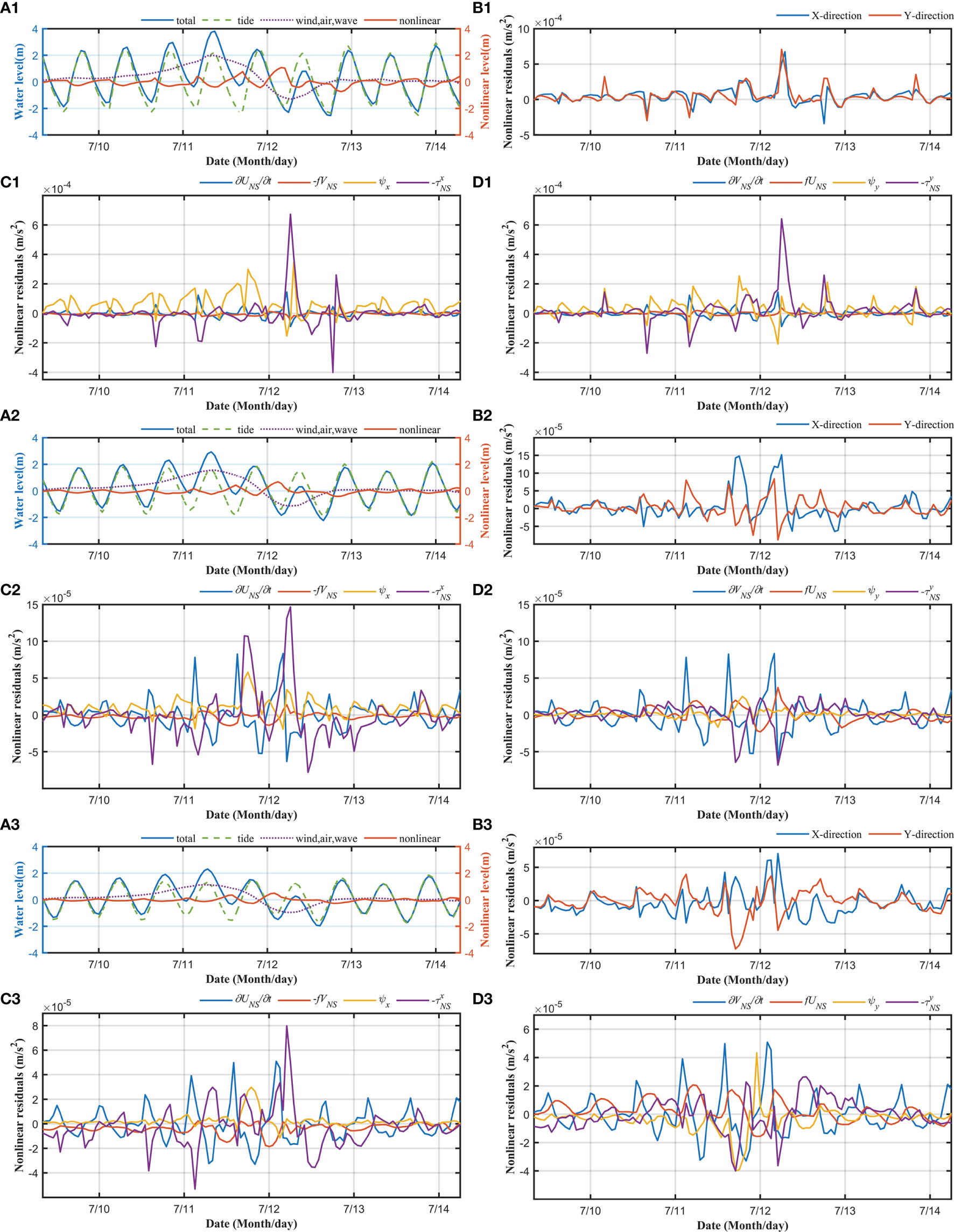
Figure 9 At station P1: (A1) Sea surface levels and surges in different cases. (B1) Sum of nonlinear surges in the x and y directions. Nonlinear components in the (C1) x direction and (D1) y direction. (A2–D2) and (A3–D3) are same as (A1–D1), but for station P2 and P3, respectively.

In the bay mouth (station P3), the nonlinear effect changes (enhance or suppress) the surge by approximately 0.5 m during the typhoon (Figure 9A1), taking approximately 50% of the total surge. The peaks of the nonlinear effects (orange line in Figure 9A1) occur in the low slack waters of the tides (green dashed line in Figure 9A1). In the x-direction (Figure 9C1), the nonlinear local acceleration and bottom friction terms dominate the nonlinear effect, followed by the convection term. In the y-direction (Figure 9D1), the nonlinear local acceleration, convection, and friction terms were dominant and had comparable magnitudes. The Coriolis force term accounts for a relatively small proportion in both the x-and y-directions (yellow line). Summarizing the components in the x-and y-directions, we obtain the sums of the nonlinear increments in the two directions (Figure 9B1). Comparing the results in the x-and y-directions with the tidal level (Figure 9A1), the nonlinear local acceleration term enhances the nonlinear surge during low slack waters and inhibits it during high slack waters.

In the middle of the bay (station P2, Figures 9A2–D2), a similar pattern occurred at station P2, but with larger magnitudes (approximately doubled), compared with those at station P1 in the bay mouth. The Coriolis term (orange line) overtook the advection term (yellow line) in the y direction (Figure 9D2).

In the upstream water channel of the bay (station P1, Figures 9A3–D3), the nonlinear local acceleration term decreased (blue line, Figures 9C3–D3). The bottom friction term (purple line) dominates the nonlinear effect, followed by the convection term (yellow line) in both the x-and y-directions (Figures 9C3–D3). The Coriolis force term accounts for a very small proportion in both the x-and y-directions.

5.2 Sensitivity Test of the Model Domain

The model domain used in this study covers less than 400 km offshore. Given a typhoon radius of ~50 km, the impact area is usually more than 500 km. Thus we tested the sensitivity of the model domain using two numerical tests. We run the model again using the same configurations in He et al. (2020) and Tang (2018) in Case 8. Base on Case 8, we changed the large domain to the small domain (Figure 1A) in Case 9. The comparison of the model results is illustrated in Figure 10.

FIGURE 10

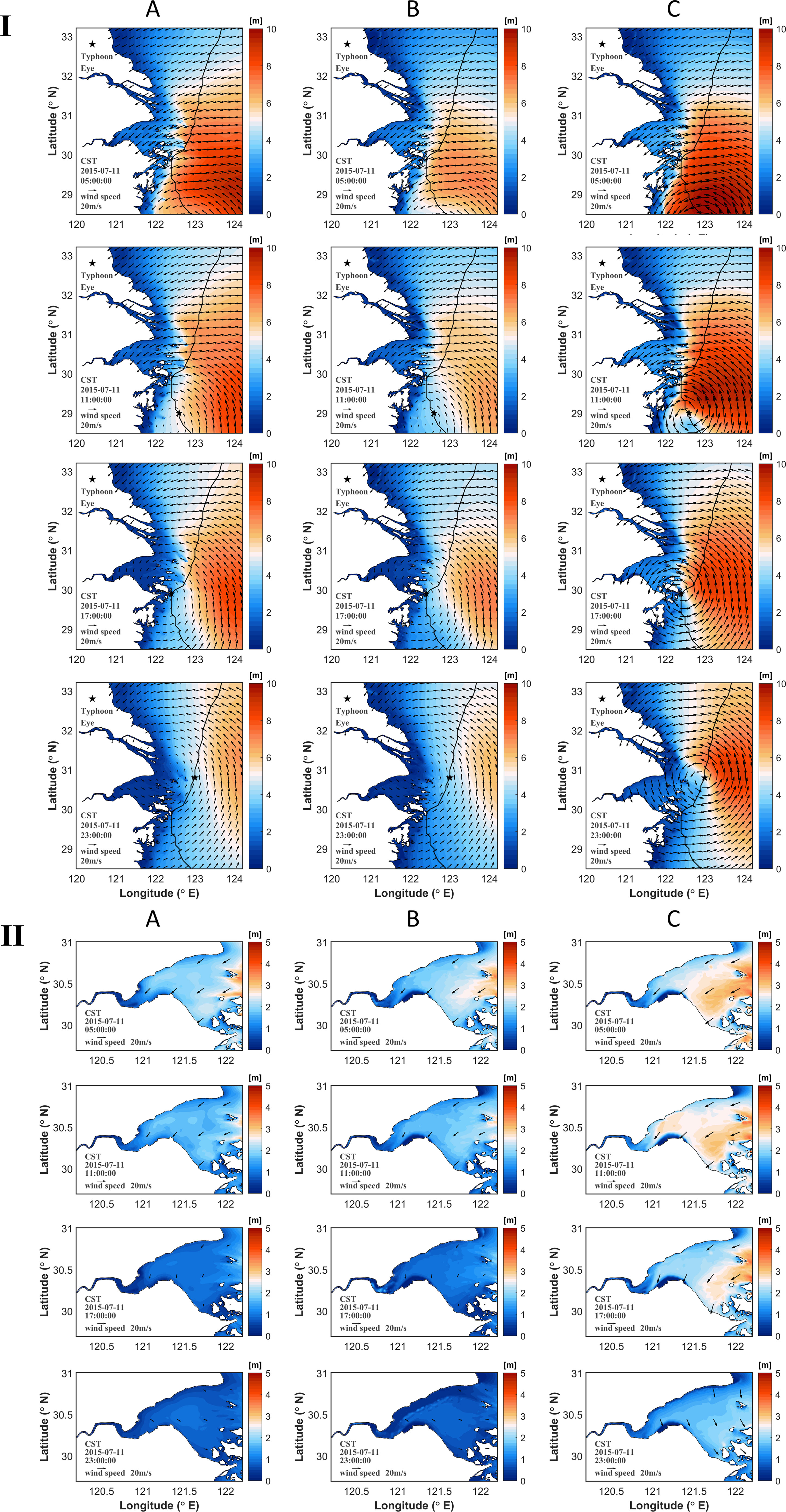
Figure 10 Significant wave heights (a) in Case 8 with the large domain in He et al. (2020), (b) in Case 9 with the small domain in Figure 1A (wind field not re-constructed), (c) in Case 0 with the small domain in Figure 1A (re-constructed wind field). Vectors indicate wind field and contours indicate significant wave heights. (I) and (II) are for the large area and the HZB, respectively.

In the open sea (Figure 10I), the significant wave heights are higher in the large domain model (Figure 10IA, Case 8) than those in the small domain model (Figure 10IB, Case 9). The significant wave heights in the small domain model with re-constructed wind field (Figure 10IC, Case 0) are slightly higher than those in Case 8. Inside the HZB (Figure 10II), the magnitudes and spatial distribution of the significant wave heights are similar in both Case 8 with large domain (Figure 10IIA) and Case 9 with small model domain (Figure 10IIB). The reconstructed wind field in Case 0 (Figure 10IIC) slightly increases the significant wave height inside the HZB.

The reconstructed wind field fit the coastal wind data better, as shown in the section 2.1.2, Yu (2020) and Ren (2022). The small domain model with reconstructed wind field reproduced the storm tide and surge well, as indicted by the model validation. Hence, we used the small model domain with reconstructed wind field (Case 0) to do the simulation in this study.

6 Conclusions

This study investigates the impacts of the super typhoon Chan-hom on hydrodynamics in the macro-tidal Hangzhou Bay (HZB) using a tide-surge-wave coupling numerical model. The wind field data of typhoon Chan-hom was reconstructed considering rotating and moving wind data. During typhoon Chan-hom, the Holland-Miyazaki method performed better in reconstructing the wind field in this study. The numerical model was fully validated using field data on sea surface levels, currents, and wave heights.

In HZB, wind stress was the main factor that dominated the storm surge, followed by the pressure surge effect, with the wave effect being the smallest. The surge caused by the wind stress of the three factors is the largest, and can reach 91.09% of the total surge, followed by air pressure, which is approximately 14.69% of the total surge, with the surge caused by waves being the smallest, only about 4.83%. The wind- and wave-included surges have an obvious tendency to gradually advance from the mouth to the top of the bay. At the mouth of the bay, they first peaked, followed by the middle of the bay and finally at the top of the bay. The pressure-induced surge was more evenly distributed in the HZB, and peaks appeared simultaneously. This is because the wind- and wave-induced surges are related to the change in the maximum wind speed radius of the typhoon, whereas the pressure surge is determined by the minimum pressure in the center of the typhoon.

Both the wind- and wave-induced surges are affected by the tidal level, and the peaks of both surges appear in the low-slack waters. The maximum wind-induced surge occurred near the peak moment of wind speed. The wave-induced surge peaks at the moment of maximum significant wave height. Both wind- and wave-induced surges occur during low slack waters. The tide-surge interaction changes (enhance or suppress) the surge by approximately 0.5 m during the typhoon, comprising approximately 50% of the total surge. Tides interact with surges via various mechanisms. The local acceleration and friction terms dominated the tide-surge interaction in the bay head, followed by the advection term. Friction and advection terms dominated at the bay head. The local acceleration term enhanced the surge in low-slack waters and suppressed it in high-slack waters.

Data Availability Statement

The original contributions presented in the study are included in the article/supplementary material. Further inquiries can be directed to the corresponding authors.

Author Contributions

LL and ZH: Manuscript writing, data analysis; methodology; modelling. ZL, ZY, and YR: Material collection; modelling; data analysis. All authors contributed to the article and approved the submitted version.

Funding

This study was partially supported by the National Key Research and Development Program of China (Grant No. 2021YFE0206200), the National Natural Science Foundation of China (41976157, 42076177), the Science Technology Department of Zhejiang Province (2021C03180, 2020C03012, U1709204).

Conflict of Interest

The authors declare that the research was conducted in the absence of any commercial or financial relationships that could be construed as a potential conflict of interest.

Publisher’s Note

All claims expressed in this article are solely those of the authors and do not necessarily represent those of their affiliated organizations, or those of the publisher, the editors and the reviewers. Any product that may be evaluated in this article, or claim that may be made by its manufacturer, is not guaranteed or endorsed by the publisher.

References

Brenner S., Gertman I., Murashkovsky A. (2007). Preoperational Ocean Forecasting in the Southeastern Mediterranean Sea: Implementation and Evaluation of the Models and Selection of the Atmospheric Forcing. J. Mar. Syst. 65 (1-4), 268–287. doi: 10.1016/j.jmarsys.2005.11.018

CrossRef Full Text | Google Scholar

Cavaleri L., Sclavo M. (2006). The Calibration of Wind and Wave Model Data in the Mediterranean Sea. Cost. Eng. 53 (7), 613–627. doi: 10.1016/j.coastaleng.2005.12.006

CrossRef Full Text | Google Scholar

Chang C., Fang H., Chen Y., Chuang S. (2015). Discussion on the Maximum Storm Radius Equations When Calculating Typhoon Waves. J. Mar. Sci. Technol. 23, 608–619.

Google Scholar

Chen C., Liu H., Beardsley R. C. (2003). An Unstructured Grid, Finite-Volume, Three-Dimensional, Primitive Equations Ocean Model: Application to Coastal Ocean and Estuaries. J. Atmosph. Ocean. Technol. 20 (1), 159–186. doi: 10.1175/1520-0426(2003)020<0159:AUGFVT>2.0.CO;2

CrossRef Full Text | Google Scholar

Chu D., Zhang J., Wu Y., Jiao X., Qian S. (2019). Sensitivities of Modelling Storm Surge to Bottom Friction, Wind Drag Coefficient, and Meteorological Product in the East China Sea. Estuar. Coast. Shelf. Sci. 231, 106460. doi: 10.1016/j.ecss.2019.106460

CrossRef Full Text | Google Scholar

Darbyshire J. (1974). Modeling Tide and Surge Interaction. Nature 249, 692–693. doi: 10.1038/249692b0

CrossRef Full Text | Google Scholar

de Vet P. L. M., van Prooijen B. C., Colosimo I., Steiner N., Ysebaert T., Herman P. M. J., et al. (2020). Variations in Storm-Induced Bed Level Dynamics Across Intertidal Flats. Sci. Rep. 10, 12877. doi: 10.1038/s41598-020-69444-7

PubMed Abstract | CrossRef Full Text | Google Scholar

Feng S. (1998). The Advance of Researches on Storm Surges, World Science-Technology Research and Development 04, 44–47. doi: 10.16507/j.issn.1006-6055.1998.04.015

CrossRef Full Text | Google Scholar

Fujita T. (1952). Pressure Distribution Within Typhoon. Geophys. Mag. 23, 437–451.

Google Scholar

Graham H. E., Nunn D. E. (1959). Meteorological Considerations Pertinent to Standard Project Hurricanes, Atlantic and Gulf Coasts of the United States, National Hurricane Research Project Report No. 33 (US Department of Commerce Washington).

Google Scholar

He Z., Tang Y., Xia Y., Chen B., Xu J., Yu Z., et al. (2020). Interaction Impacts of Tides, Waves and Winds on Storm Surge in a Channel-Island System: Observational and Numerical Study in Yangshan Harbor. Ocean. Dynam. 70 (3), 307–325. doi: 10.1007/s10236-019-01328-5

CrossRef Full Text | Google Scholar

Holland G. J. (1980). An Analytic Model of the Wind and Pressure Profiles in Hurricanes. Month. Weather. Rev. 108 (8), 1212–1218. doi: 10.1175/1520-0493(1980)108<1212:AAMOTW>2.0.CO;2

CrossRef Full Text | Google Scholar

Horsburgh K. J., Wilson C. (2007). Tide-Surge Interaction and its Role in the Distribution of Surge Residuals in the North Sea. J. Geophys. Res. Ocean. 112. doi: 10.1029/2006JC004033

CrossRef Full Text | Google Scholar

Jelesnianski C. P. (1965). A Numerical Calculation of Storm Tides Induced by a Tropical Storm Impinging on a Continental Shelf. Month. Weather. Rev. 93 (6), 343–358. doi: 10.1175/1520-0493(1993)093<0343:ANCOS>2.3.CO;2

CrossRef Full Text | Google Scholar

Jelesnianski C. P. (1966). Numerical Computations of Storm Surges Without Bottom Stress. Month. Weather. Rev. 94 (6), 379–394. doi: 10.1175/1520-0493(1966)094<0379:NCOSSW>2.3.CO;2

CrossRef Full Text | Google Scholar

Jiang Z., Hua F., Ping Q. (2008). A New Scheme for Adjusting the Tropical Cyclone Parameters. Adv. Mar. Sci. 01), 1–7.

Google Scholar

Jones J. E., Davies A. M. (2007). Influence of non-Linear Effects Upon Surge Elevations Along the West Coast of Britain. Ocean. Dynam. 57 (4-5), 401–416. doi: 10.1007/s10236-007-0119-0

CrossRef Full Text | Google Scholar

Knaff J. A., Sampson C. R., Musgrave K. D. (2018). Statistical Tropical Cyclone Wind Radii Prediction Using Climatology and Persistence: Updates for the Western North Pacific. Weather. Forecast. 33 (4), 1093–1098. doi: 10.1175/WAF-D-18-0027.1

CrossRef Full Text | Google Scholar

Knaff J. A., Sampson C. R., DeMaria M., Marchok T. P., Gross J. M., McAdie C.J., et al. (2007). Statistical Tropical Cyclone Wind Radii Prediction Using Climatology and Persistence, Weather and Forecasting. 22 (24), 781–91 doi: 10.1175/WAF1026.1

CrossRef Full Text | Google Scholar

Li R. (2007). Prediction of Typhoon Extreme Wind Speed Based on Improved Typhoon Key Parameters, Harbin Institute of Technology. Harbin, China.

Google Scholar

Lin N., Chavas D. (2012). On Hurricane Parametric Wind and Applications in Storm Surge Modeling. J. Geophys. Res.: Atmosph. 117, D09120. doi: 10.1029/2011JD017126

CrossRef Full Text | Google Scholar

Lin N., Emanuel K., Oppenheimer M., Vanmarcke E. (2012). Physically Based Assessment of Hurricane Surge Threat Under Climate Change. Nat. Climate Change 2, 462–467. doi: 10.1038/nclimate1389

CrossRef Full Text | Google Scholar

Lu X., Yu H., Ying M., Zhao B., Zhang S., Lin L., et al. (2021). Western North Pacific Tropical Cyclone Database Created by the China Meteorological Administration. Adv. Atmosph. Sci. 38 (4), 690–699. doi: 10.1007/s00376-020-0211-7

CrossRef Full Text | Google Scholar

Lv X., Yuan D., Ma X., Tao J. (2014). Wave Characteristics Analysis in Bohai Sea Based on ECMWF Wind Field. Ocean. Eng. 91, 159–171. doi: 10.1016/j.oceaneng.2014.09.010

CrossRef Full Text | Google Scholar

Marsooli R., Lin N., Emanuel K., Feng K. (2019). Climate Change Exacerbates Hurricane Flood Hazards Along US Atlantic and Gulf Coasts in Spatially Varying Patterns. Nat. Commun. 10, 3785. doi: 10.1038/s41467-019-11755-z

PubMed Abstract | CrossRef Full Text | Google Scholar

Miyazaki M, Ueno T, Unoki S (1962). Theoretical Investigations of Typhoon Surges Along the Japanese Coast. Oceanographic Magazine 13 (2), 103–118. doi: 10.1016/0011-7471(63)90458

CrossRef Full Text | Google Scholar

Murphy A. H. (1992). Climatology, Persistence, and Their Linear Combination as Standards of Reference in Skill Scores. Weather. Forecast. 4 (7), 692–698. doi: 10.1175/1520-0434(1992)007<0692:CPATLC>2.0.CO;2

CrossRef Full Text | Google Scholar

Ni Y., Geng Z., Zhu J. (2003). Study on Characteristic of Hydrodynamics in Hangzhou Bay. J. Hydrodynam. (A). 18 (4), 439–445.

Google Scholar

Olbert A. I., Nash S., Cunnane C., Hartnett M. (2013). Tide-Surge Interactions and Their Effects on Total Sea Levels in Irish Coastal Waters. Ocean. Dynam. 63 (6), 599–614. doi: 10.1007/s10236-013-0618-0

CrossRef Full Text | Google Scholar

Pan Y., Chen Y., Li J., Ding X. (2016). Improvement of Wind Field Hindcasts for Tropical Cyclones. Water Sci. Eng. 9 (1), 58–66. doi: 10.1016/j.wse.2016.02.002

CrossRef Full Text | Google Scholar

Rego J. L., Li C. (2010). Nonlinear Terms in Storm Surge Predictions: Effect of Tide and Shelf Geometry With Case Study From Hurricane Rita. J. Geophys. Res. 115, C06020. doi: 10.1029/2009JC005285

CrossRef Full Text | Google Scholar

Ren Y. (2022). Asymmetric Characteristics and Mechanism of Suspended Sediment in Hangzhou Bay Considering Wave-Current Interaction (Hangzhou, China:Zhejiang University).

Google Scholar

Shankar C. G., Behera M. R. (2021). Numerical Analysis on the Effect of Wave Boundary Condition in Storm Wave and Surge Modeling for a Tropical Cyclonic Condition. Ocean. Eng. 220, 108371. doi: 10.1016/j.oceaneng.2020.108371

CrossRef Full Text | Google Scholar

Shen Z. (2018). Numerical Simulation of Storm Surges in the Bohai Sea (Dalian, China: Dalian University of Technology).

Google Scholar

Shen J., Gong W. (2009). Influence of Model Domain Size, Wind Directions and Ekman Transport on Storm Surge Development Inside the Chesapeake Bay: A Case Study of Extratropical Cyclone Ernest. J. Mar. Syst. 75 (1-2), 198–215. doi: 10.1016/j.jmarsys.2008.09.001

CrossRef Full Text | Google Scholar

Signell R. P., Carniel S., Cavaleri L., Chiggiato J., Doyle J. D., Pullen J., et al. (2005). Assessment of Wind Quality for Oceanographic Modelling in Semi-Enclosed Basins. J. Mar. Syst. 53 (1-4), 217–233. doi: 10.1016/j.jmarsys.2004.03.006

CrossRef Full Text | Google Scholar

Tang Y. (2018). Numerical Simulation of Characteristics of Storm Tide in Yangshan Harbor Based on Tide-Surge-Wave Model, Master Thesis (Hangzhou, China:Zhejiang University).

Google Scholar

Thuy N. B., Kim S., Anh T. N., Cuong N. K., Thuc P. T., Hole L. R. (2020). The Influence of Moving Speeds, Wind Speeds, and Sea Level Pressures on After-Runner Storm Surges in the Gulf of Tonkin, Vietnam. Ocean. Eng. 212, 107613. doi: 10.1016/j.oceaneng.2020.107613

CrossRef Full Text | Google Scholar

Torres M., Hashemi M., Scott H., Spaulding M., Ginis I., Grilli S. (2019). Role of Hurricane Wind Models in Accurate Simulation of Storm Surge and Waves. J. Waterway. Port. Coast. Ocean. Eng. 145 (1), 1–17. doi: 10.1061/(ASCE)WW.1943-5460.0000496

CrossRef Full Text | Google Scholar

Tu J., Fan D. (2017). Flow and Turbulence Structure in a Hypertidal Estuary With the World’s Biggest Tidal Bore. J. Geophys. Research-Ocean. 122, 3417–3433. doi: 10.1002/2016JC012120

CrossRef Full Text | Google Scholar

Ueno T. (1981). Numerical Computations of the Storm Surges in Tosa Bay. J. Oceanog. Soc. Japan. 37 (2), 61–73. doi: 10.1007/BF02072559

CrossRef Full Text | Google Scholar

Wang Q., Pan C., Pan D. (2021). Numerical Study of the Effect of Typhoon Yagi on the Qiantang River Tidal Bore. Region. Stud. Mar. Sci. 44, 101780. doi: 10.1016/j.rsma.2021.101780

CrossRef Full Text | Google Scholar

Wang S., Pan C., Xie D., Xu M., Yan Y., Li X. (2022). Grain Size Characteristics of Surface Sediment and its Response to the Dynamic Sedimentary Environment in Qiantang Estuary, China. Int. J. Sediment. Res. 37 (4), 457–468. doi: 10.1016/j.ijsrc.2021.12.002

CrossRef Full Text | Google Scholar

Wang P., Sheng J. (2020). Effects of Wave-Induced Vertical Reynolds Stress on Upper-Ocean Momentum Transfer Over the Scotian Shelf During Extreme Weather Events. Region. Stud. Mar. Sci. 33, 100954. doi: 10.1016/j.rsma.2019.100954

CrossRef Full Text | Google Scholar

Wang X., Yin Q., Zhang B. (1991). Research and Applications of a Forecasting Model of Typhoon Surges in China Seas. Adv. Water Sci. 2 (1), 1–10.

Google Scholar

Wei K., Arwade S. R., Myers A. T., Valamanesh V., Pang W. (2017). Effect of Wind and Wave Directionality on the Structural Performance of Non-Operational Offshore Wind Turbines Supported by Jackets During Hurricanes. Wind Energ. 20, 289–303. doi: 10.1002/we.2006

CrossRef Full Text | Google Scholar

Wei K., Shen Z., Wu L., Qin S. (2019). Coupled Numerical Simulation on Wave and Storm Surge in Coastal Areas Under Strong Typhoons. Eng. Mechanics. 36 (11), 139–146.

Google Scholar

Wolf J. (1978). Interaction of Tide and Surge in a Semi-Infinite Uniform Channel, With Application Io Surge Propagation Down the East Coast of Britain. Appl. Math. 2 (4), 245–253.

Google Scholar

Xie D., Gao S., Wang Z. B., Pan C., Wu X., Wang Q. (2017b). Morphodynamic Modeling of a Large Inside Sandbar and its Dextral Morphology in a Convergent Estuary: Qiantang Estuary, China. J. Geophys. Res. Earth Surface. 122. doi: 10.1002/2017JF004293

CrossRef Full Text | Google Scholar

Xie D., Pan C., Gao S., Wang Z. (2018). Morphodynamics of the Qiantang Estuary, China: Controls of River Flood Events and Tidal Bores. Mar. Geol. 406, 27–33. doi: 10.1016/j.margeo.2018.09.003

CrossRef Full Text | Google Scholar

Xie D., Pan C., Wu X., Gao S., Wang Z. (2017a). Local Human Activities Overwhelm Decreased Sediment Supply From the Changjiang River: Continued Rapid Accumulation in the Hangzhou Bay-Qiantang Estuary System. Mar. Geol. 392, 66–77. doi: 10.1016/j.margeo.2017.08.013

CrossRef Full Text | Google Scholar

Xie D., Wang Z., Gao S., et al. (2009). Modeling the Tidal Channel Morphodynamics in a Macro-Tidal Embayment, Hangzhou Bay, China. Continent. Shelf. Res. 29 (15), 1757–1767. doi: 10.1016/j.csr.2009.03.009

CrossRef Full Text | Google Scholar

Yang W., Yin B., Feng X., Yang E., Gao G., Chen H. (2019). The Effect of Nonlinear Factors on Tide-Surge Interaction: A Case Study of Typhoon Rammasun in Tieshan Bay, China. Estuar. Coast. Shelf. Sci. 219, 420–428. doi: 10.1016/j.ecss.2019.01.024

CrossRef Full Text | Google Scholar

Ye T. (2019). The Multi-Scale Variations of Suspended Sediment Dynamics in Hangzhou Bay and its Interaction With Tidal Flat Variations (Zhejiang University).

Google Scholar

Ying M., Zhang W., Yu H., Lu X., Feng J., Fan Y., et al. (2014). An Overview of the China Meteorological Administration Tropical Cyclone Database. J. Atmosph. Ocean. Technol. 31 (2), 287–301. doi: 10.1175/JTECH-D-12-00119.1

CrossRef Full Text | Google Scholar

Yu Z. (2020). Hydrodynamics and Sediment Transport During Typhoon in the Hangzhou Bay, Master Thesis (Hangzhou, China: Zhejiang University).

Google Scholar

Zhang H., Cheng W., Qiu X., Feng X., Gong W. (2017). Tide-Surge Interaction Along the East Coast of the Leizhou Peninsula, South China Sea. Continent. Shelf. Res. 142, 32–49. doi: 10.1016/j.csr.2017.05.015

CrossRef Full Text | Google Scholar

Zhang H., Sheng J. (2015). Examination of Extreme Sea Levels Due to Storm Surges and Tides Over the Northwest Pacific Ocean. Continent. Shelf. Res. 93, 81–97. doi: 10.1016/j.csr.2014.12.001

CrossRef Full Text | Google Scholar

Zhang W., Shi F., Hong H., Shang S., Kirby J. T. (2010). Tide-Surge Interaction Intensified by the Taiwan Strait. J. Geophys. Res. 115, C06012. doi: 10.1029/2009JC005762

CrossRef Full Text | Google Scholar

Zhang W., Teng L., Zhang J., Xiong M., Yin C. (2019). Numerical Study on Effect of Tidal Phase on Storm Surge in the South Yellow Sea. J. Oceanol. Limnol. 37 (6), 2037–2055. doi: 10.1007/s00343-019-8277-8

CrossRef Full Text | Google Scholar

Zhong S. (2019). Improved Wind-Field-Based Simulation of Storm Surge in Zhoushan Fishery Harbor (Hangzhou, China: Zhejiang University).

Google Scholar

Zhou T, Tan Y, Chu A., Zhang C (2018). Integrated Model for Astronomic Tide and Storm Surge Induced by Typhoon for Ningbo Coast. Paper presented at the The 28th International Ocean and Polar Engineering Conference, Sapporo, Japan, June 2018.

Google Scholar