Striped marlin in their Pacific Ocean milieu: Vertical movements and habitats vary with time and place

Striped marlin, Kajikia audax, a top bycatch of the longline fishery, has been designated as being in overfished condition in the Western and Central North Pacific, and overfishing is still occurring. This prompts an urgent need to devise conservation and management measures based on the best, current information on the biology and ecology of this species. Despite decades of conventional tagging around the Hawaiian waters, ecological research on striped marlin in the Central North Pacific has been lacking since 2005, and little is known about striped marlin’s vertical habitat, diving behavior and bycatch vulnerability in this area. To address this knowledge void, 31 popup satellite archival tags (4 X-Tags; Microwave Telemetry, Inc. and 27 MiniPATs; Wildlife Computers Inc.) were deployed on striped marlin (138-192 cm eye fork length) between 2016 and 2019 via the Hawaii-based longline fleet. Transmitted time series records revealed striped marlin spent 38 and 81% of their day and night in the top 5 m, with median daytime and night depths of 44 m and 2 m, respectively. Temperatures experienced were 23.3°C, daytime median, and 24.6°C, nighttime median, to a minimum of 7.6°C at the deepest depth logged, 472 m. Striped marlin exhibited distinct swimming behaviors, including diel depth distributions, excursions around the top of the thermocline, and extended time at the surface, most likely reflecting the dynamic biophysical environment and intrinsic life history of this highly migratory predator. High post-release survivorship (86%) in tagged striped marlin, and their predominant use of the sea surface and mixed layer indicate that live release measures can be a viable bycatch reduction strategy.

Introduction

Striped marlin, Kajikia audax, is a widely recognized denizen of the epipelagic zone that makes infrequent, short excursions into the thermocline (Bernal et al., 2010). Despite being characterized as restricted to the mixed layer either by low temperature (Brill et al., 1993) or dissolved oxygen (DO) concentration (Prince and Goodyear, 2006), striped marlin are capable of withstanding physiologically-limiting conditions for brief periods (Lam et al., 2015). Striped marlin could utilize this ability in an oxygen-depleted setting to exploit prey that are not tolerant of low dissolved oxygen, such as in the Gulf of California or off the southern tip of Baja California (Lam et al., 2015) In these environments where DO at 100 m was ≤2 ml L^-1 (Lam et al., 2015) and a persistent chlorophyll-a maximum found between 40 and 190 m (Márquez-Artavia et al., 2019), striped marlin exhibited oscillatory behavior, or “yo-yo” dives, from the surface to right above or below the top of the thermocline (~50 m). This type of repetitive swimming, also observed for the great white shark (Nasby-Lucas et al., 2009), may represent one of multiple foraging strategies that striped marlin adapt and deploy while hunting a myriad of epipelagic, mesopelagic and benthic prey (Abitia-Cárdenas et al., 2011; Ordiano-Flores et al., 2021). An appreciation of their foraging ecology and swimming behaviors in the context of a changing biophysical environment can improve understanding of striped marlin’s vulnerability to different fishing gears, and potentially, reduce harmful incidental fisheries interactions.

As a key bycatch species in pelagic fisheries targeting tuna and swordfish (WPRFMC, 2021), striped marlin have been in overfished condition in the Western and Central North Pacific since the mid-1990s (ISC, 2019; Sculley, 2021). Consequently, new conservation management measures may be forthcoming, despite the lack of well-resolved information on migration and habitat in the Central North Pacific, where the Hawaiian longline fleet operates. Fishery independent information for striped marlin is rare, and conventional tagging effort around Hawaii is almost nonexistent north of 22°N and south of 15°N (Bromhead et al., 2004). Similarly, electronic tagging and tracking of any kind is confined to a single, local acoustic study (Brill et al., 1993) and one popup satellite archival tag (PSAT) study (Domeier, 2006), representing only tens of hours of sonic tracking and less than four months of PSAT logging, for a total of twelve individuals. Against the massive scale of the Pacific fisheries (Sala et al., 2018), high vulnerability to fishing mortality (Rodríguez et al., 2021) and striped marlin’s overfished status, this is decidedly insufficient spatiotemporal and behavioral information to best inform its management and conservation. Our objective is to utilize PSAT data to provide an up-to-date habitat characterization for striped marlin intercepted by the Hawaii-based longline fishery. A companion study (Lam et al., 2022) highlights horizontal dispersal patterns, connectivity, and oceanographic regions occupied by striped marlin. Our work here delineates striped marlin occupancy preferences and swimming behavior in order to provide more robust sampling of their water column use and oceanographic preferences around Hawaii and in the wider Central North Pacific during times of overfishing, changing climate and shifting ecosystems (Clarke et al., 2021).

Materials and methods

Electronic tagging

Thirty-one PSATs (4 X-Tags; Microwave Telemetry, Inc. and 27 MiniPATs; Wildlife Computers Inc.) were deployed on striped marlin between 2016 and 2019 by Hawaii-based longline vessels operating in the Central North Pacific. Upon retrieval of a set, an individual that was assessed to be in good condition was tagged on deck (n = 2) or along the side of the boat via a custom-built tagging pole (n = 29). Hooks were either removed, or fishing line cut as close to the jaw as possible prior to release. Tag tethers and anchors were constructed according to materials and methods developed for bluefin tuna tagging (Lutcavage et al., 1999; Galuardi and Lutcavage, 2012), and have shown great efficacy on sailfish (Lam et al., 2016). The tagger implanted the black nylon “umbrella” dart through the musculature, into the pterygiophores at the anterior dorsal region. For fish tagged alongside the vessel, whole weight (W) was estimated by the vessel’s captain to the nearest five pounds (1 lb ~ 0.4536 kg). Eye fork length (EFL) was measured to the nearest centimeter for fish tagged on deck. W (in kg) was converted to EFL (in cm) or lower jaw fork length (LJFL, in cm) following Sun et al. (2011):

$\begin{array}{ll}W=4.68\times {10}^{-6}EF{L}^{3.16}& (1)\end{array}$

and

$\begin{array}{ll}LJFL=1.12EFL+7.33& (2)\end{array}$

Data acquisition

PSATs were programmed to record relative light level, external temperature, pressure (depth) for 12 month missions. Archived depth and temperature time series were sub-sampled to 5-minute (MiniPAT) and 15-minute (X-Tag) resolution by manufacturer routines for satellite transmission through the Argos-2 services, which limit each transmitted message to 32 bytes (W.M.O., 2018). Manufacturer routines also treated depth and temperature time series as separate data streams, so retrieved satellite messages might contain unsynchronized depth and temperature records (i.e., non-matching date-time stamps). In addition, satellite data retrieval does not guarantee delivery of all collected records, and the quantity of returned data can be highly variable (Musyl et al., 2011). Any breaks in the data recovery also create gaps in the time series. For MiniPAT, we programmed the tags to “always transmit” both depth and temperature time series, as enabling any “on-off” transmission schedule (i.e., duty-cycle) would exacerbate data mismatches in time.

All tags had a failsafe release if the tag experienced any constant depth for 3 (X-Tag) or 4 (MiniPAT) days, a hallmark of post-release mortality or tag shedding. MiniPAT firmware also included detection and transmission of a hardware failure message (“pin broke”) indicating that the tag’s nosecone pin had broken, separating the tag from its tether, causing premature release. Once a tag popped off and began transmitting, positions with Argos location classes LC 1, 2, and 3 were noted, and the first of these positions was selected as the tag’s reporting position.

Logger sensor data

Returned data were imported into and managed through Tagbase (Lam and Tsontos, 2011). Predation-associated impacts did not damage any of the released tags or its antenna, and provided data for deducing the plausible fate of the tagged individual. Predator interaction was inferred if sensor data indicated ingestion, including sustained low light levels, increased temperature indicative of a warm-bodied predator, and depth pattern changes.

Transmitted light data represented either truncated light curves around (MiniPAT) or detected time stamps of (X-Tag) sunrise and sunset. From this light information, geolocation was only performed on fish carrying tags for over 14 days (Lam et al., 2022). Protocols are detailed in Appendix 1. We defined biologged depth and temperature records as day or night, based on sunset and sunrise times recorded by X-tags and estimated for MiniPATs by the geolocation routine, TrackIt (Lam et al., 2010). From the estimated latitudes, depth and temperature records were aggregated at 10° bands to generate summary statistics.

Lunar phase and fraction illuminated were obtained with R package, suncalc (github.com/datastorm-open/suncalc). We then used linear mixed-effects models to investigate the effects of fraction of the moon illuminated on the interquartile range or maximum of daily nighttime depth, using individual fish as a fixed effect. Models were built by R package, nlme (cran.r-project.org/web/packages/nlme/index.html).

Since data were only returned via satellites (i.e., no downloaded archive from a physically recovered PSAT), gaps in the depth and temperature time series were unavoidable. To reduce the influence of missing or incongruous data on the construction of depth-temperature profiles and percentage time-at-depth histograms, we aggregated time series records at 5-day intervals for each MiniPAT. Within a given 5-day period, a regression spline was fitted through the daytime depths and temperatures using R package, splines (Perperoglou et al., 2019). This 5-day window was chosen after experimenting with various time intervals (3-14 d) to produce smoothed depth-temperature profiles. For percentage time-at-depth histograms, depth records were binned at 10-m intervals by day and night. Based on the depth distribution relative to a corresponding depth-temperature profile, we visually determined if there was a prominent use of the top 10 m, mixed layer and thermocline during a given 5-day period by the tagged marlin. Cluster analysis and other automated classification techniques were applied, but failed to isolate meaningful patterns, likely due to the irregular presence of gaps in the time series. Any visually identified depth pattern was then investigated with linear mixed-effects models. Possible effects of month, 10°-latitude band and lunar illumination on the frequency of occurrence of a depth pattern were examined using individual fish as a fixed effect. Lastly, two measures of vertical activity, in addition to mean depth, were generated hourly for each tagged fish: vertical cumulative distance (Vdist) is the sum of all unsigned depth changes between successive time points, and vertical net displacement (Vplace) is the sum of all signed depth changes between successive time points. A large Vdist reflects a fish that frequently swam up and down in the water column, while a positive Vplace means at the end of an hour, the fish was at a deeper depth than at the beginning of the hour.

Oceanographic and biological information

To aid the interpretation of fish movement, the following geographical information system resources were accessed: bathymetric values from Smith & Sandwell Topography (0.0167° resolution, version 11.1), sea surface height (variable ‘zos’) and temperature (variable ‘thetao’) monthly mean values [product ID GLOBAL_REANALYSIS_PHY_001_030] from the Copernicus Marine Service Global Monitoring and Forecasting Centre (CMEMS; marine.copernicus.eu). Additionally, daily sea surface temperature (SST) [product ID METOFFICE-GLO-SST-L4-NRT-OBS-SST-MON-V2]. Mixed layer depth (MLD) was extracted along reconstructed tracks from NCEP Global Ocean Data Assimilation System monthly data (psl.noaa.gov/data/gridded/data.godas.html), which defines MLD as the depth where the buoyancy difference with respect to the surface level is equal to 0.03 cm s^-2.

With the understanding that PSATs do not identify or confirm spawning, we evaluated changes in vertical movement (mean depth, Vdist, Vplace) that might be associated with spawning habitats during the spawning season. Since it wasn’t possible to assign reproductive status of released fish, we referenced the maturity ogive developed by NOAA Pacific Islands Fisheries Science Center (PIFSC) observer sampling program (Humphreys and Brodziak, 2019; Humphreys and Brodziak, 2021). PIFSC determined that active spawning females (n = 37, 151-188 cm EFL) were concentrated in a T-shaped area (between 25-30°N & 150-165°W, and 20-25°N & 155-160°W; see Appendix 1) from May to July. The boundary of this active spawning area was included in our analysis of vertical movement with respect to life history requirements.

Results

After removing tags that failed to report (n = 8) or did not return sufficient messages via satellites (n = 2), logger sensor data from 21 individuals were available (Table 1). Whole weight of these striped marlin was 34 ± 4 kg (mean ± sd) and length was 148 ± 5 cm EFL. Tracks were successfully reconstructed for 17 fish, providing the spatial context for our investigation into their vertical movements (Appendix 1). Two predation events were observed for striped marlin within four days after release, and two additional mortalities occurred between 58 and 106 days post-release (Table 2). All predator interactions occurred far from the Main Hawaiian Islands (MHI) in pelagic waters with 22.3-24.3°C SST, and at depths below 40 m (Table 2). Based on maximum attained depth and temperature elevated above ambient during the tag ingestion period, predators were most likely sharks or other billfishes. Apart from the two fish that were predated within four days of release, one other fish sank after two days, yielding an overall post-release survivorship of tagged fish of 86% (19 out of 22).

TABLE 1

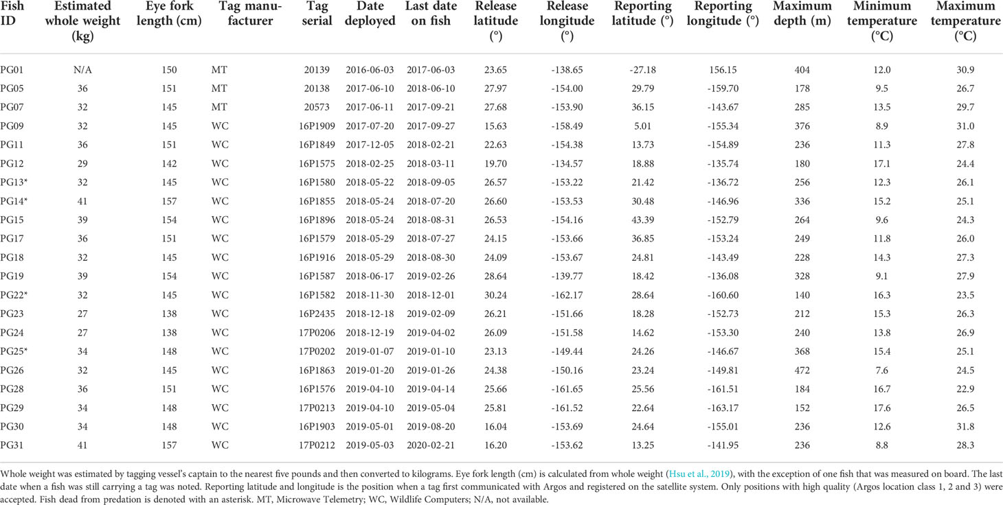
Table 1 Tagging and data summary for striped marlin, Kajikia audax.

TABLE 2

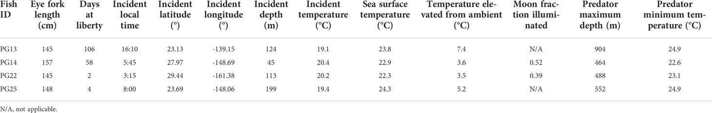
Table 2 Predator interactions that resulted in fish mortality.

Vertical habitat

From cumulative depth distributions (Figure 1), striped marlin spent 38 and 81% of their day and night, respectively, in the top 5 m. Swimming depths were 90% encapsulated within 120 and 37 m during day and night, respectively. Their median (interquartile range, IQR) daytime and nighttime depths were 44 m (2-82) and 2 m (0-3), respectively, with significant differences in diel depth and temperature occupancy (two-sample Kolmogorov–Smirnov test, p < 0.0001). Linear mixed effects models found no significant relationship between fraction of the moon illuminated and daily nighttime depth IQR (p = 0.06) or maximum depth (p = 0.79). The majority of mixed layer depths associated with striped marlin tracks were between 46 and 83 m (50-90% of all available records). Median daytime temperature was 23.3°C (IQR = 20.8-24.5) and 24.6°C (IQR = 23.6-25.4), nighttime. Tagged marlin experienced SSTs of 16.9-30.9°C, mirroring their nighttime temperature range. However, during the day a shift to cooler temperatures occurred, in which 90% of records fell within 12-26.7°C. Pooling all data, striped marlin experienced ambient temperatures between 7.6 and 31.8°C (Table 1).

FIGURE 1

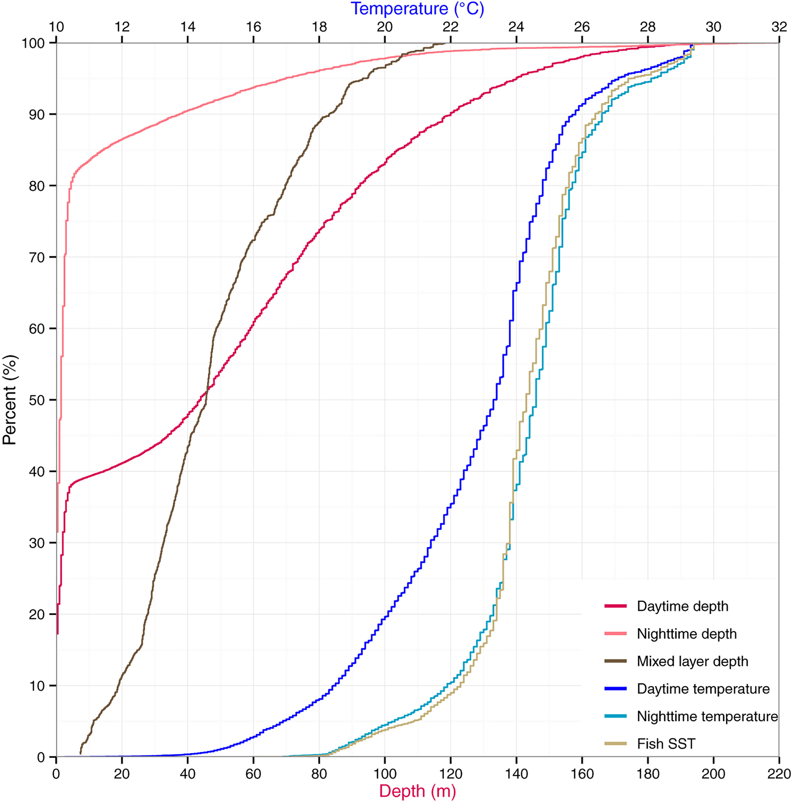
Figure 1 Vertical habitat of striped marlin. Depth and temperature are expressed as cumulative percentages for daytime and nighttime. Daily sea surface temperature (Fish SST) and mixed layer depth are also summarized.

Even as fish remained near the surface throughout the day they showed marked diel shifts in depth distribution and temperature across their ranges (Figure 2; Table 3). In daytime, tagged fish ventured to the top of the thermocline, except between 40 and 50°N, where temperatures experienced were cooler, near 19°C (Figure 2). A reduction in vertical habitat at 40-50°N was reflected by a shallow mean depth (7.9 m) and the smallest depth IQR (9.5 m, Table 3). In 10-30°N where most tagged fish ventured, they spent 24-34% of their time below the mixed layer (mean: 46-69 m; Table 3), reaching 100-150 m (Figure 2). Below 10°N, they reduced their time in the top 5 m, and shifted daytime occupancy to 40-60 m, right above the base of the mixed layer, where temperatures were at least 0.5-1°C cooler than at the surface (Figure 2). Mean mixed layer depth varied between 12 and 91 m across striped marlin’s range (Figure 2), with MLD being the shallowest at latitudes >30°N and deepening southwards (Table 3). On average, in the Central North Pacific striped marlin spent 27% of their time below the mixed layer (Table 3). Pairwise comparisons of logged depth and temperature records via Wilcoxon rank sum test revealed significant differences (p< 0.001) among all 10°-latitude bands.

FIGURE 2

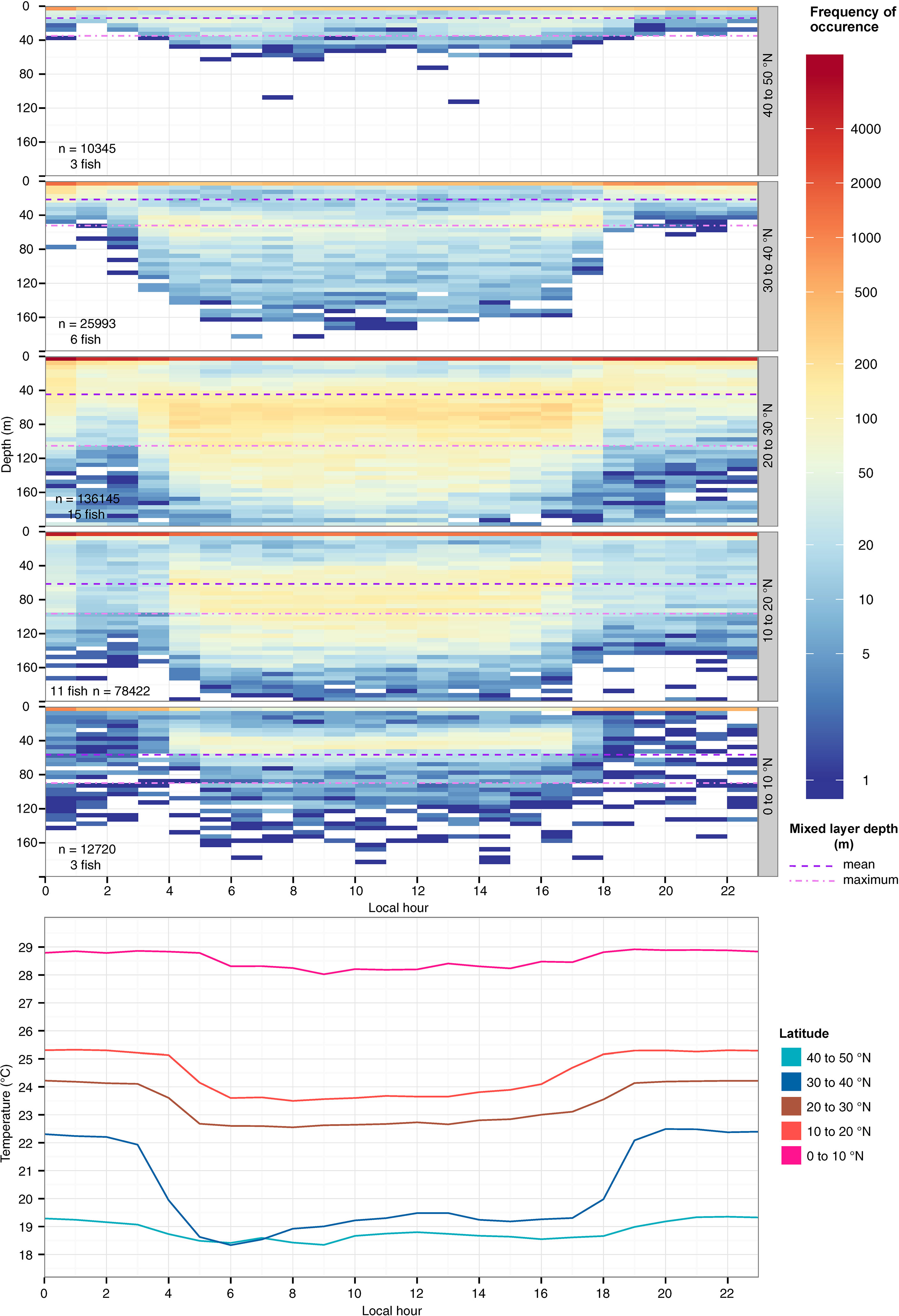
Figure 2 Hourly depth distribution (top) and mean temperature (bottom) of striped marlin over a 24-hour period at 10°-latitudinal bands. Colors in logarithmic scale represent frequency of occurrence (i.e., count). The number of samples and individuals contributing to the depth distribution are indicated in each panel. Mean (violet dashed line) and maximum (lavender dotted line) values for the mixed layer depth at each latitude band are shown. Depths were binned every 5 m and values deeper than 200 m were aggregated into the 200-m bin.

TABLE 3

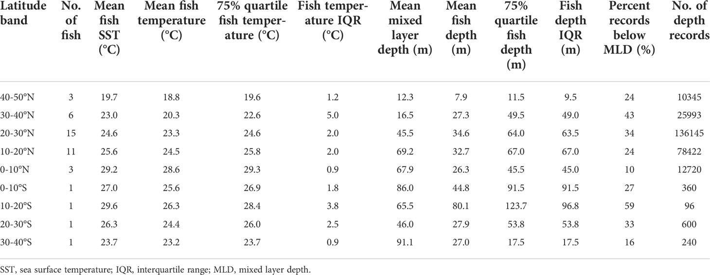
Table 3 Depth occupied and temperature experienced by striped marlin summarized by 10°-latitude bands.

Maximum depth recorded among all tagged marlin was 472 m (Table 1), but daily maximum depths varied with location (Figure 3), with fish reaching depths >200 m over a large area along Molokai Fracture Zone between 120-150°W, and south of 10°N. In contrast, north of 35°N, their vertical habitat was compressed, maximum depths were mostly above 100 m (Figure 3), depth IQR was narrower than those at the tropics (Table 3), and they spent little time below 80 m (Figure 2). During the first-ever documented dispersal to the Southern Hemisphere (Lam et al., 2022), between 5 and 20°S, PG01 logged a series of daily maximum depths >200 m during January 2017 (Figure 3), while elsewhere, its mean daily maximum depth was 141 m (Table 4). At that time PG01 had the largest latitudinal range (19.6°) (Table 4), and the highest daily movement rate (90 km day^-1) among all tagged fish.

FIGURE 3

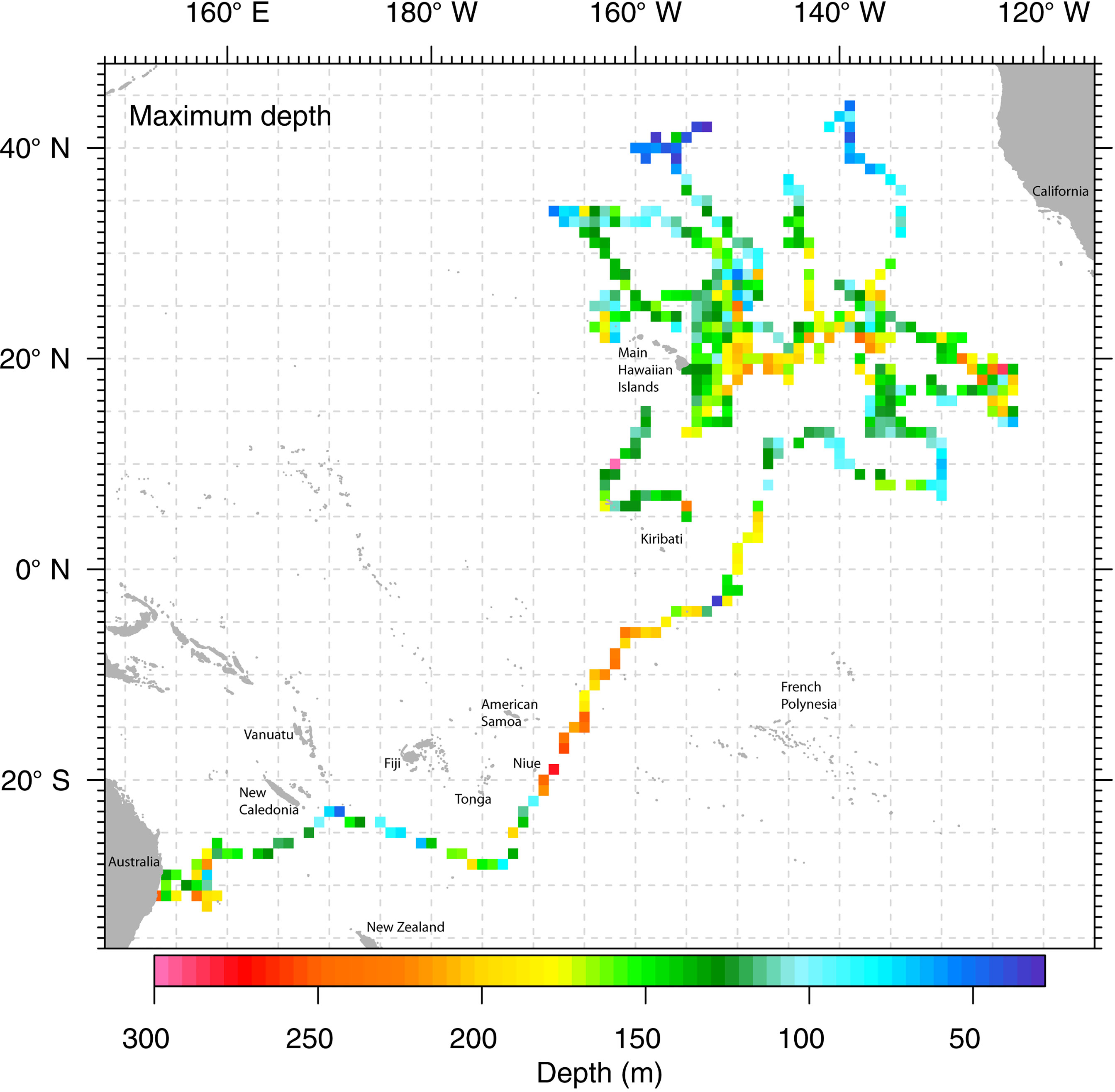
Figure 3 Maximum depth of striped marlin along their dispersal tracks. Tag-recorded maximum depths are binned in a 1°x1° grid and plotted in false color. When multiple values exist in a grid cell, the maximum value among them is represented.

TABLE 4

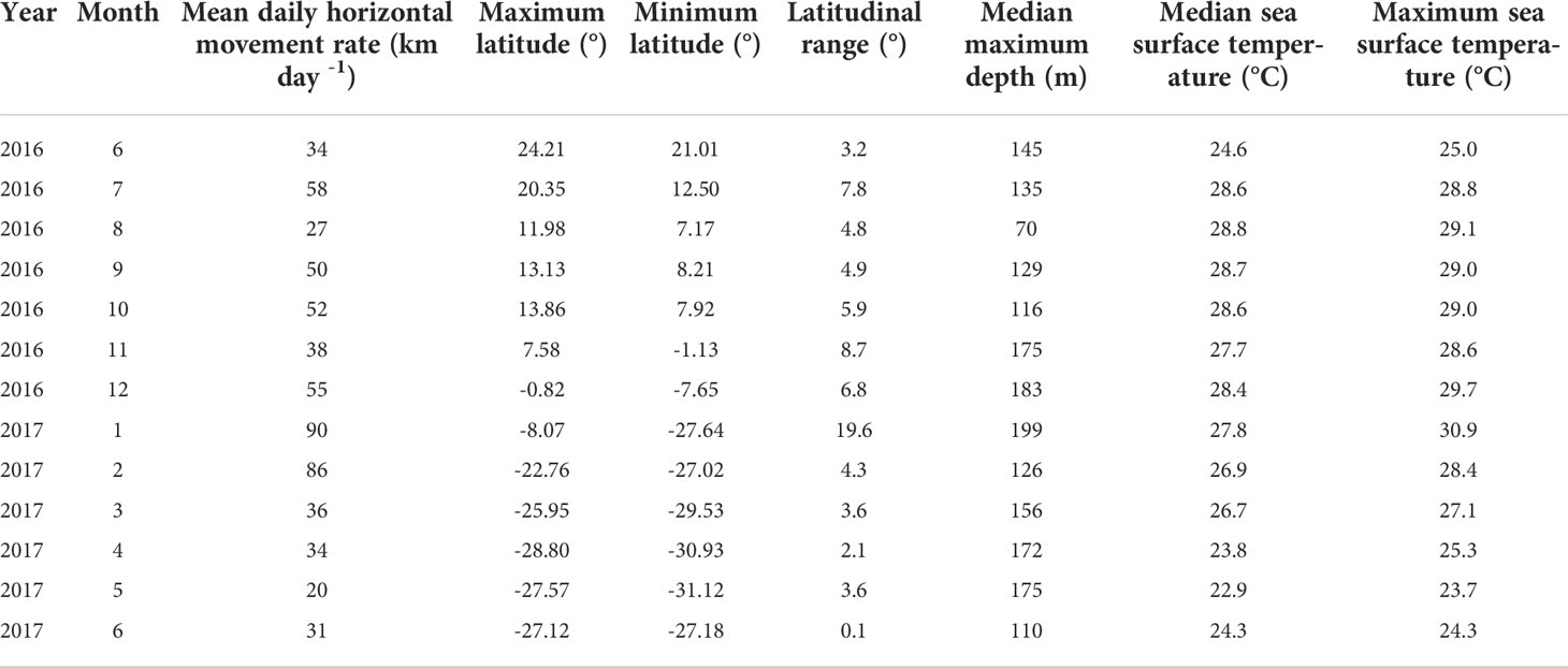
Table 4 Monthly daily horizontal movement rate of PG01 in relation to its latitudinal range, maximum depth and sea surface temperature experienced.

Swimming behavior and vertical activity

Striped marlin exhibited three common patterns in their swimming depths (Appendix 2). Pattern 1 is characterized by a fish staying near the sea surface for extended periods, which occurred more often during the night (Figures 4, 5A). Pattern 2 features a high occupancy of the thermocline during day and night, either through brief (sometimes repetitive) trips from the surface or oscillatory movements within the thermocline (Figures 4, 5B, D). Pattern 3 is marked by multiple trips to different depths within the mixed layer, from the surface or ascents from the thermocline (Figures 4, 5A, C, D).

FIGURE 4

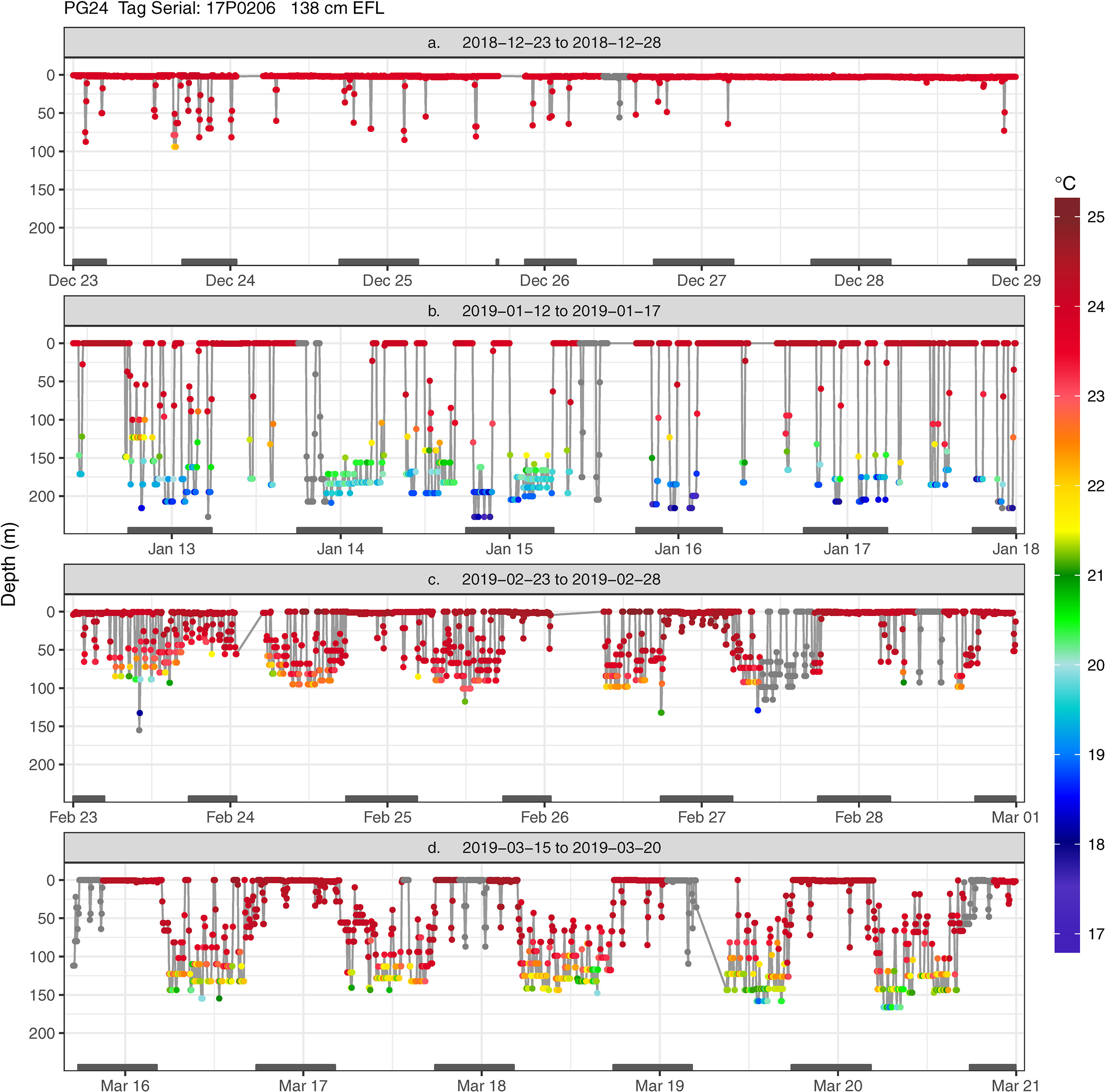
Figure 4 Transmitted depth and temperature time series of striped marlin PG24 from (A) 2018-12-23 to 2018-12-28, (B) 2019-01-12 to 2019-01-17, (C) 2019-02-23 to 2019-02-28, and (D) 2019-03-15 to 2019-03-20. When temperature values were not received through the Argos satellites, corresponding depth values are shown in grey. Grey bars on the x-axis (date scale) denote nighttime.

FIGURE 5

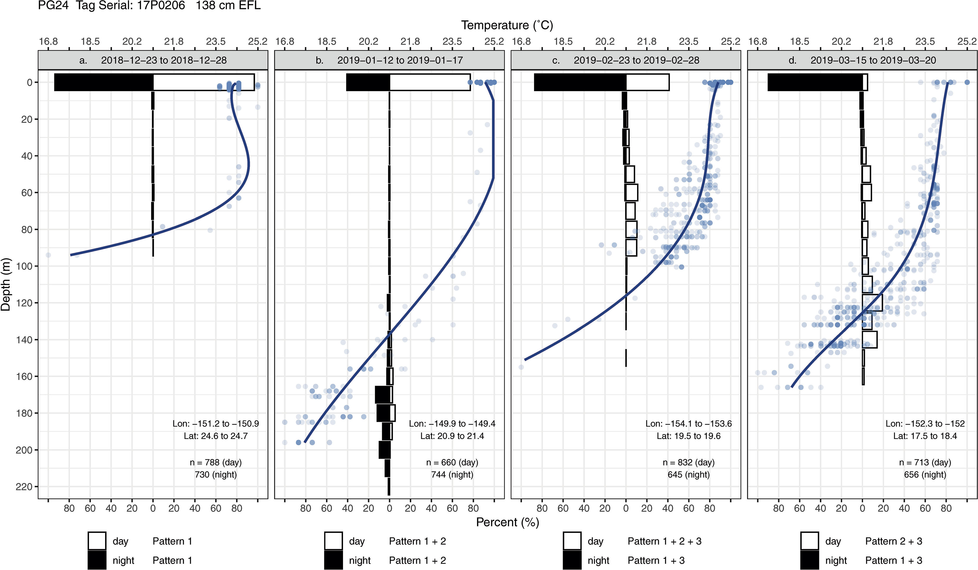
Figure 5 Diel time-at-depth histograms and daytime depth-temperature profiles of striped marlin PG24 from (A) 2018-12-23 to 2018-12-28, (B) 2019-01-12 to 2019-01-17, (C) 2019-02-23 to 2019-02-28, and (D) 2019-03-15 to 2019-03-20. In the histograms, depths were binned at every 10 m. Depth-temperature values (blue dots) in each period were also fitted with a regression spline to construct a smoothed profile (thick blue line). Depth patterns were identified for day and night: Pattern 1 is characterized by a fish staying near the sea surface for extended periods; Pattern 2 features a high occupancy of the thermocline, either through brief (sometimes repetitive) trips from the surface or oscillatory movements within the thermocline; Pattern 3 is marked by multiple trips to various depths within the mixed layer either from the surface or from the thermocline.

For daytime, forays into the thermocline (Pattern 2) and occupancy near the surface (Pattern 1) were most frequent, and with lower frequency, movements within the mixed layer (Pattern 3) (Appendix 3). Interestingly, during the day striped marlin often spent little time at the surface when in fracture zones and the vicinity of seamounts (Figures 4, 5D). For example, before PG31’s light sensor failed in late December, it had transited multiple geological features (Appendix 1), including Geologist Seamounts, Northwestern Hawaiian Islands, Molokai Fracture Zone, Murray Fracture Zone, and Clarion Fracture Zone over seven months. Upon arrival at each area, PG31 reduced its time near the surface and spent the majority of daytime in the thermocline. This pattern disappeared when PG31 moved to an area lacking prominent geological features (Appendices 2, 3). For nighttime, striped marlin utilized the surface (Pattern 1) and mixed layer (Pattern 3) (Appendix 3). Striped marlin sometimes frequented the thermocline during night (Pattern 2) (Figures 4, 5B) during all lunar phases (Appendix 3). Linear mixed-effects models did not find any significant relationship between the identified depth patterns (during day or night) with month, latitudinal band or lunar illumination.

Together, these depth patterns and swimming behaviors were often maintained for 1 to 2- weeks before marlin switched to another behavior (Appendix 2). For example, for two weeks in mid-December, PG24 initially stayed near the sea surface, making few descents (Figure 6A) but near the Molokai Fracture Zone, it switched to depths below the thermocline (150-240 m) while heading west along the fracture (Figure 4B). Its mid-January hourly vertical net displacement (Vplace) ranged between -20 to +20 m, i.e., movements began and ended at similar depths (Figure 6B). A corresponding high vertical cumulative distance (Vdist) signaled repeated descents and ascents, i.e., a “yo-yo” or oscillatory pattern. Between early and mid-February, this fish transited the Wini Seamount and southeast of the Puna Ridge where it descended to the bottom of the mixed layer (~120 m) and to the thermocline. In late February PG24 spent daylight just below the mixed layer, around 100 m (Figures 4, 6C), and then extended to 120 m in mid-late March (Figure 4D) near the Bryan Seamount. There, a high Vdist was a result of trips from the mixed layer to ~50 m and back (Figure 6D), while over the entire track, Vplace generally delineated dawn descents and dusk ascents.

FIGURE 6

Figure 6 Vertical activity of striped marlin PG24. Hourly mean depth (top), vertical cumulative distance, Vdist (middle), and vertical net displacement, Vplace (bottom) are summarized through a 24-hours period (00:00-23:00 local time) for its tracked time at liberty (x-axis). False-color scale is shared by all three variables, but each has its own break values for mean depth (left), Vdist (middle), and Vplace (right). Labels added to the top and bottom of the color scale illustrate what each variable physically represents, e.g., deeper vs. shallower depth. Latitude of its track positions through time (x-axis) is shown on the secondary y-axis as a white trace. Grey bars along the x-axis denote the same time periods shown previously in Figure 4: (A) 2018-12-23 to 2018-12-28, (B) 2019-01-12 to 2019-01-17, (C) 2019-02-23 to 2019-02-28, and (D) 2019-03-15 to 2019-03-20. Black ticks on the x-axis denote the dates in which over 95% of the moon was illuminated.

Movements on known spawning grounds

A fish’s presence on spawning grounds during documented peak spawning, together with favorable environmental conditions (e.g., 24°C SST) suggests that reproductive behavior is likely. For instance, in early June PG14 (157 cm EFL) was positioned at the edges of a cyclonic eddy on the spawning ground northeast of the MHI (Figure 7A). While there, PG14 shifted from using the mixed layer during the day to staying near the sea surface in >24°C for about one week (Figure 7B) before reverting to diel vertical behavior (Figure 7C). Eight other individuals (Appendix 1) also transited the spawning ground between May and June, but did not provide sufficient time series data for a similar analysis of their vertical behavior.

FIGURE 7

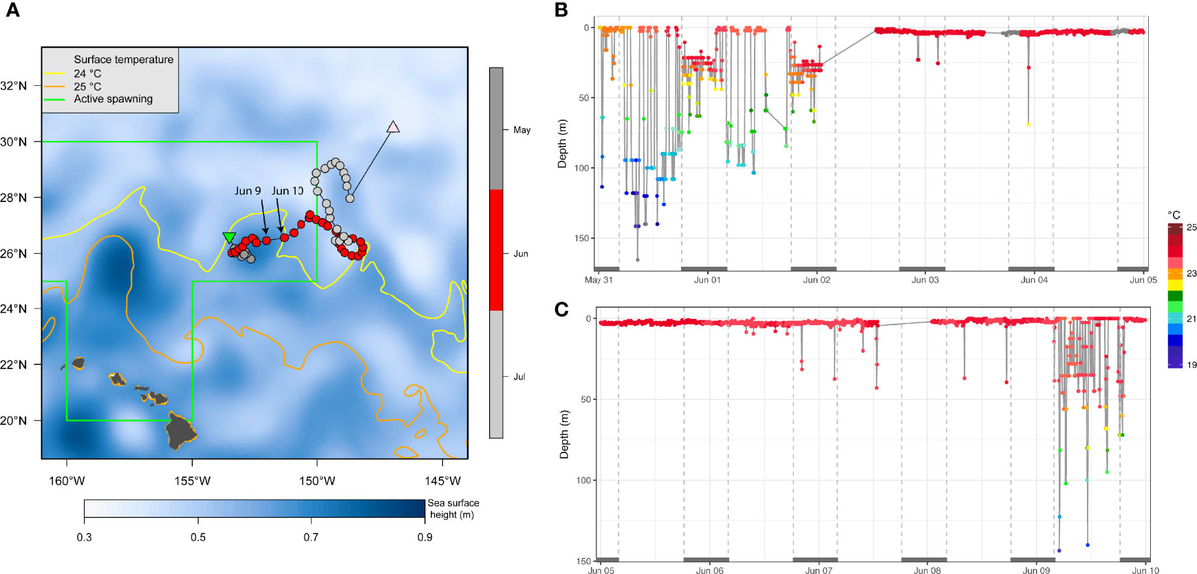
Figure 7 Oceanographic setting (A) and swimming depth-temperature time series (B, C) of striped marlin PG14 in early June. In (A), sea surface height is plotted as false-color, and surface temperature isotherms at 24°C (yellow) and 25°C (orange) are contoured, using monthly data of June 2018 from GLOBAL_REANALYSIS_PHY_001_030 product of the Copernicus Marine Service Global Monitoring and Forecasting Centre. Positions are color-coded by month. The area depicting location of sampled active female spawners (Humphreys and Brodziak, 2019) during the spawning season (May-August) is outlined in green. In (B, C), when temperature values were not received through the Argos satellites, corresponding depth values are shown in grey. Grey bars on the x-axis (date scale) denote nighttime.

Discussion

Here we report the most comprehensive effort to date characterizing vertical movements of striped marlin in the Central North Pacific, accompanied by complementary analysis of their horizontal dispersals and oceanographic associations (Lam et al., 2022). Although our findings of vertical habitat and behavior were mostly consistent with studies elsewhere in the Pacific, more extensive and current insights on depth preferences in this and other studies can better inform development of productive management and bycatch mitigation measures. Tagged striped marlin frequently used the thermocline in daytime, especially around seamounts and fracture zones, but occasionally at night. This subtlety can be overlooked when summary statistics show mainly near-surface and/or mixed layer occupancy (Sippel et al., 2007; Lam et al., 2015). Moreover, that striped marlin regularly shifted depth patterns across time and location demonstrated adaptive use of the water column, likely in response to local foraging opportunities. Considering that striped marlin are known to rush at a sardine school near the sea surface (Hansen et al., 2020), they might use the same hunting strategy at boundary conditions, namely at the top of and in the thermocline and oxycline (Lam et al., 2015) to exploit a diverse selection of prey (Abitia-Cárdenas et al., 1997; Shimose et al., 2010; Ortega Garcia et al., 2017). This would reduce competition with other top predators through trophic niche separation (Acosta-Pachón and Ortega-García, 2019; Rosas-Luis et al., 2021). Application of accelerometer-coupled infra-red cameras (Cade et al., 2021), once minimization is achieved, might provide the bio-logging advances necessary to uncover the secrets of striped marlin hunting and other behavior at depths.

Navigation

Beyond foraging, the function of exemplary, deep “dives” undertaken by marlin and tuna is not well explained, nor are all the sensory systems that might be appropriated for guiding information gathering in darker, cooler ocean depths. Curiously, PG01 reached depths >200 m during its rapid transit through the West Pacific Warm Pool (~0-20°S; Wyrtki, 1989 but not elsewhere. The coarse resolution of light-based geolocation positions of PSATs (Galuardi and Lam, 2014) had precluded a detailed exploration of PG01’s deeper forays with environmental and bathymetric features. However, descents ≥250 m were also observed in four satellite-linked striped marlin tagged off New Zealand that abruptly reversed travel directions when they reached 20-21°S and increased transit speed away from the area (Sippel et al., 2011). The authors suggested that such a reversal, an apparent avoidance, may contribute to the long-established fishery pattern of a low catch-per-unit-effort between 10-20°S (Squire and Suzuki, 1990). Similarly, PG01’s elevated movement rate and deeper descents in the same region (Table 4) provided another possible example of shared movement dynamics contributing to the observed spatial structuring in catch distribution.

Periodic deep descents also occur in Atlantic bluefin tuna, which make deepest “bounce” dives on the shelf at dusk and dawn (Lutcavage et al., 2000) and descents >500 m at the Gulf Stream margins (Galuardi et al., 2010). Deep descents plausibly serve a navigational purpose: magnetic orientation was proposed in pioneering tracking studies of shark and tuna (Carey and Scharold, 1990; Klimley, 1993), and supported by studies of potential bio-physical sensory mechanisms via brain magnetite particles (Walker et al., 1997; Walker and Dennis, 2005). More recently, Horton et al. (2017) presented compelling evidence in satellite-tracked marine mammals and great white sharks that gravitational and magnetic cues detected through variations within the water column and from bathymetric features (e.g., seamounts, ridges) can be integrated with astronomical cues (e.g., lunar illumination) detected near or at the sea surface to form a navigational system. Tuna, billfish and shark navigate with surprising accuracy, and return to apparently favored locations after crossing vast ocean distances (Carey and Scharold, 1990; Galuardi et al., 2010; Keller et al., 2021). This extraordinary phenomenon points to a long-standing gap in scientific understanding, especially that of neuro-sensory mechanisms (Dudchenko and Wallace, 2018; Watts et al., 2018), memory (Mouritsen, 2018) and collective behavior (Couzin, 2018). Although speculative at present, vertical transits of the water column can represent an important, yet untapped dimension of vertebrate sensory systems, and have potential to expose navigational secrets of highly migratory fishes. These sensory capabilities may remain undetected if only horizontal movement and migration are considered (Martin, 2018).

Management considerations

Our successful partnership with fishermen collaborators has enabled new insights into water column utilization of striped marlin across vast stretches of the open ocean where they could likely interact with longline gear of the US and international fleets. Occupancy of different parts of the water column by time of day (e.g., Figure 1) can be incorporated in models of fishery catch-per-unit-effort data to derive indices of relative abundance (Maunder et al., 2006; Johnson et al., 2019), or be used to evaluate gear vulnerability by capture time (Boggs, 1992; Rodrigues et al., 2022). In designing effective management measures, authorities must strike a balance between the economic benefits of fishing harvest, species conservative priorities and climate impacts (Mckuin et al., 2021). Mandatory live release is a mitigation measure applicable to both the shallow-set and deep-set longline fishery, on the account of a high survivorship (Pine et al., 2008). In this study, only two tagged fish died within 4 days of release (Table 1), similar to other PSAT-tagged striped marlin released off New Zealand by the recreational fleet (Sippel et al., 2011). Our vertical data records confirmed that striped marlin regularly frequented the top 5 m of the water column, and 90% of their swimming depths were above 120 m. Additionally, at higher latitudes (>30°N), striped marlin were mostly located above 40 m (Figure 2), so removing shallow (<120 m) hooks from deep-set longline in such locations might reduce striped marlin fishing mortality. While economic impacts of hook removal for bigeye tuna caught at deeper depths appeared minimal (Boggs, 1992; Beverly et al., 2009), similar cost-benefit analysis and potential spillover effects among multi-national fleets (Chan and Pan, 2016) need to be re-examined as spatiotemporal changes in the vertical habitat of striped marlin were common. Consequently, there may be advantages to specifying time- and area-based conservation measure (Jensen et al., 2010; Hilborn et al., 2022; Pons et al., 2022), such as applying particular mitigation approaches in the main spawning area during peak spawning months. As vertical and horizontal movement preferences of striped marlin and other bycatch species are further resolved, management and conservation objectives could be achieved by deploying more targeted measures, with input of the fleets and fisheries experts in regard to the best practices (Hare, 2020).

Life history perspectives

Most of our tagged fish were close to length at 50% maturity of 153.6 cm EFL (Humphreys and Brodziak, 2021), and larger than the smallest spawning female (146 cm) in Humphreys and Brodziak (2019). Given their fast growth rate at this age range (Kanaiwa et al., 2020), it’s reasonable to project that tagged individuals would reach spawning-capable size during their tracked time-at-liberty. While it’s impossible to directly observe reproductive behaviors given current tag hardware and geolocation limitations, we postulate that prolonged departures from diel swimming, to a pattern of extended time spent near the surface on a spawning ground, during the spawning season, may signal a behavioral switch from foraging to reproduction (Figure 7). While we couldn’t explicitly detect frequency of potential spawning bouts from our data, if surface occupancy were related to spawning or courtship, events would likely repeat on striped marlin’s average spawn of every 3-10 days (Kopf et al., 2012; Chang et al., 2018), and at least 27-90 times over a single season (Kopf et al., 2012). Multiple periods of surface occupancy were observed for PG14 throughout June and July, especially when it traveled along the edges of areas with an elevated sea surface height (Appendix 4). Common knowledge among fishers and fish buyers on the auction floor is that some striped marlin appear with orange colored, high-quality, lipid-rich flesh (Figure S1) between April and June, which may reflect primed somatic condition just prior to the start of the spawning season, or a unique prey choice during this time of the year. Notably, the highest Fulton’s condition factor (K) was recorded in April in mature female striped marlin off Taiwan, prior to the peak spawning months of June and July (Chang et al., 2018). Collectively, these reproductive characteristics provide multiple lines of evidence that some of the tagged fish could be spawning-capable, or approaching spawning during their tracked duration.

Conclusions

Striped marlin tagged in the Central North Pacific exhibited a strong preference for the epipelagic zone, much like conspecifics that aggregated around islands, coastal areas and on continental shelves. Distinct swimming patterns were displayed in different locations, months and environmental conditions that could reflect various life history activities, from foraging runs targeting preferred prey, to surface-based behaviors signaling potential reproductive activities on known spawning ground. Understanding where, when and how these activities occur can contribute to a far better understanding of their biology, physiology and life history. These goals also call for improved, reliable and cost effective tag and tracking technologies that surpass current tools and observational capabilities. Filling these scientific gaps will improve our ability to design management measures that are more effective towards the sustainable harvest of bigeye tuna and swordfish, and a reduction of incidental catch of non-target species like the striped marlin.

Data Availability Statement

The raw data supporting the conclusions of this article will be made available by the authors, without undue reservation.

Ethics Statement

Ethical review and approval were not required for the animal study because in the US, it is accepted practice that placing a dart type external fish tag aboard a commercial fishing vessel does not require review by IAUC committees. Tag and release, with a small bio-compatible dart, conducted in the manner stated in our paper, is routine in US recreational and commercial fisheries, and does not require permitting by fisheries regulators.

Author Contributions

CL, ML, and CT designed and executed the research; CL performed the analyses. All authors prepared, revised and approved the manuscript.

Funding

We are grateful to the funding provided by NOAA Saltonstall-Kennedy Grant (award # NA15NMF4270324).

Acknowledgments

We are indebted to our tagging partners, Capts. Steve Sexton, Tim Jones, Steve Gates, Joel Ralston and their crews, without whom this work would not have been possible.

Conflict of Interest

The authors declare that the research was conducted in the absence of any commercial or financial relationships that could be construed as a potential conflict of interest.

Publisher’s Note

All claims expressed in this article are solely those of the authors and do not necessarily represent those of their affiliated organizations, or those of the publisher, the editors and the reviewers. Any product that may be evaluated in this article, or claim that may be made by its manufacturer, is not guaranteed or endorsed by the publisher.

Supplementary Material

The Supplementary Material for this article can be found online at: https://www.frontiersin.org/articles/10.3389/fmars.2022.879503/full#supplementary-material

Supplementary Figure 1 | Coloration of harvested striped marlin muscle. Tail cuts of two landed striped marlin show different coloration (right). “Pumpkin” colored orange flesh is observed among high-quality landed fish between April and June (left).

References

Abitia-Cárdenas L. A., Galván-Magaña F., Cruz-Escalona V. H., Peterson M. S., Rodríguez-Romero J. (2011). Daily food intake of Kajikia audax (Philippi 1887) off Cabo San Lucas, Gulf of California, Mexico. Latin Am. J. Aquat. Res. 39, 449–460. doi: 10.3856/vol39-issue3-fulltext-6

CrossRef Full Text | Google Scholar

Abitia-Cárdenas L. A., Galván-Magaña F., Rodriguez-Romero J. (1997). Food habits and energy values of prey of striped marlin, Tetrapturus audax, off the coast of Mexico. Fishery Bull. 95, 360–368.

Google Scholar

Acosta-Pachón T. A., Ortega-García S. (2019). Trophic interaction between striped marlin and swordfish using different timescales in waters around Baja Cal. Sur, Mexico. Mar. Biol. Res. 15, 97–112. doi: 10.1080/17451000.2019.1578377

CrossRef Full Text | Google Scholar

Bernal D., Sepulveda C., Musyl M., Brill R. (2010). “The eco-physiology of swimming and movement patterns of tunas, billfishes, and large pelagic sharks,” in Fish Locomotion - an etho-ecological perspective. Eds. Domenici P., Kapurr D. (Enfield, New Hampshire: Scientific Publishers), 436–483 pp.

Google Scholar

Beverly S., Curran D., Musyl M., Molony B. (2009). Effects of eliminating shallow hooks from tuna longline sets on target and non-target species in the Hawaii-based pelagic tuna fishery. Fisheries Res. 96, 281–288. doi: 10.1016/j.fishres.2008.12.010

CrossRef Full Text | Google Scholar

Boggs C. H. (1992). Depth, capture time, and hooked longevity of longline-caught pelagic fish - timing bites of fish with chips. Fishery Bull. 90, 642–658.

Google Scholar

Brill R. W., Holts D. B., Chang R. K. C., Sullivan S., Dewar H., Carey F. G. (1993). Vertical and horizontal movements of striped marlin (Tetrapturus audax) near the Hawaiian-islands, determined by ultrasonic telemetry, with simultaneous measurement of oceanic currents. Mar. Biol. 117, 567–574. doi: 10.1007/BF00349767

CrossRef Full Text | Google Scholar

Bromhead D., Pepperell J., Wise B., Findlay J. (2004). Striped marlin: biology and fisheries. final report to the Australian fisheries management authority and the fisheries research fund (Canberra, Australia: Bureau of Rural Sciences).

Google Scholar

Cade D. E., Gough W. T., Czapanskiy M. F., Fahlbusch J. A., Kahane-Rapport S. R., Linsky J. M. J., et al. (2021). Tools for integrating inertial sensor data with video bio-loggers, including estimation of animal orientation, motion, and position. Anim. Biotelemetry 9, 34. doi: 10.1186/s40317-021-00256-w

CrossRef Full Text | Google Scholar

Carey F. G., Scharold J. V. (1990). Movements of blue sharks (Prionace glauca) in depth and course. Mar. Biol. 106, 329–342. doi: 10.1007/BF01344309

CrossRef Full Text | Google Scholar

Chang H.-Y., Sun C.-L., Yeh S.-Z., Chang Y.-J., Su N.-J., Dinardo G. (2018). Reproductive biology of female striped marlin Kajikia audax in the western Pacific Ocean. J. Fish Biol. 92, 105–130. doi: 10.1111/jfb.13497

PubMed Abstract | CrossRef Full Text | Google Scholar

Chan H. L., Pan M. (2016). Spillover effects of environmental regulation for Sea turtle protection in the Hawaii longline swordfish fishery. Mar. Resource Economics 31, 259–279. doi: 10.1086/686672

CrossRef Full Text | Google Scholar

Clarke T. M., Reygondeau G., Wabnitz C., Robertson R., Ixquiac-Cabrera M., López M., et al. (2021). Climate change impacts on living marine resources in the eastern tropical Pacific. Diversity Distributions 27, 65–81. doi: 10.1111/ddi.13181

CrossRef Full Text | Google Scholar

Couzin I. D. (2018). Collective animal migration. Curr. Biol. 28, R976–R980. doi: 10.1016/j.cub.2018.04.044

PubMed Abstract | CrossRef Full Text | Google Scholar

Domeier M. L. (2006). An analysis of Pacific striped marlin (Tetrapturus audax) horizontal movement patterns using pop-up satellite archival tags. Bull. Mar. Sci. 79, 811–825(815).

Google Scholar

Dudchenko P. A., Wallace D. (2018). Neuroethology of spatial cognition. Curr. Biol. 28, R988–R992. doi: 10.1016/j.cub.2018.04.051

PubMed Abstract | CrossRef Full Text | Google Scholar

Galuardi B., Lam C. H. (2014). “Telemetry analysis of highly migratory species,” in Stock identification methods (Second edition). Eds. Cadrin S. X., Kerr L. A., Mariani S. (San Diego: Academic Press), 447–476 pp.

Google Scholar

Galuardi B., Lutcavage M. (2012). Dispersal routes and habitat utilization of juvenile Atlantic bluefin tuna, Thunnus thynnus, tracked with mini PSAT and archival tags. PLos One 7, e37829. doi: 10.1371/journal.pone.0037829

PubMed Abstract | CrossRef Full Text | Google Scholar

Galuardi B., Royer F., Golet W., Logan J., Neilson J., Lutcavage M. (2010). Complex migration routes of Atlantic bluefin tuna (Thunnus thynnus) question current population structure paradigm. Can. J. Fisheries Aquat. Sci. 67, 966–976. doi: 10.1139/F10-033

CrossRef Full Text | Google Scholar

Hansen M., Krause S., Breuker M., Kurvers R. H., Dhellemmes F., Viblanc P., et al. (2020). Linking hunting weaponry to attack strategies in sailfish and striped marlin. Proc. R. Soc. B 287, 20192228. doi: 10.1098/rspb.2019.2228

CrossRef Full Text | Google Scholar

Hare J. A. (2020). Ten lessons from the frontlines of science in support of fisheries management. ICES J. Mar. Sci. 77, 870–877. doi: 10.1093/icesjms/fsaa025

CrossRef Full Text | Google Scholar

Hilborn R., Agostini V. N., Chaloupka M., Garcia S. M., Gerber L. R., Gilman E., et al. (2022). Area-based management of blue water fisheries: Current knowledge and research needs. Fish Fisheries 23, 492–518. doi: 10.1111/faf.12629

CrossRef Full Text | Google Scholar

Horton T. W., Hauser N., Zerbini A. N., Francis M. P., Domeier M. L., Andriolo A., et al. (2017). Route fidelity during marine megafauna migration. Front. Mar. Sci. 4. doi: 10.3389/fmars.2017.00422s

CrossRef Full Text | Google Scholar

Hsu J., Chang Y. J., Yeh S. Y., Sun C. L., Yeh S. Z. (2019). Catch and size data of striped marlin (Kajikia audax) by the Taiwanese fisheries in the Western and Central North Pacific Ocean during 1958-2017 (Honolulu, USA: ISC/19/BILLWG), 11 pp. 1/03.

Google Scholar

Humphreys R., Brodziak J. (2019). Reproductive maturity of striped marlin, Kajikia audax, in the Central North Pacific off Hawaii (Honolulu, USA: ISC/19/BILLWG), 29 pp. 2/02.

Google Scholar

Humphreys R., Brodziak J. (2021). Revised analyses of the reproductive maturity of female striped marlin, Kajikia audax, in the Central North Pacific off Hawaii Vol. 13 (ISC/21/BILLWG), 39 pp. 3/07Webminar.

Google Scholar

ISC (2019). “Stock assessment report for striped marlin (Kajikia audax) in the Western and Central North Pacific Ocean through 2017,” in 19th Meeting of the International Scientific Committee for Tuna and Tuna-Like Species in the Central North Pacific Ocean Taipei, Taiwan July 11-15, 2019, Annex. 11. 11:91

Google Scholar

Jensen O. P., Ortega-Garcia S., Martell S. J. D., Ahrens R. N. M., Domeier M. L., Walters C. J., et al. (2010). Local management of a "highly migratory species": The effects of long-line closures and recreational catch-and-release for Baja California striped marlin fisheries. Prog. In Oceanography 86, 176–186. doi: 10.1016/j.pocean.2010.04.020

CrossRef Full Text | Google Scholar

Johnson K. F., Thorson J. T., Punt A. E. (2019). Investigating the value of including depth during spatiotemporal index standardization. Fisheries Res. 216, 126–137. doi: 10.1016/j.fishres.2019.04.004

CrossRef Full Text | Google Scholar

Kanaiwa M., Sato Y., Ijima H., Kurashima A., Shimose T., Kanaiwa M. (2020). Review and working plan of re-estimation for growth curve of swordfish and striped marlin in North Pacific Ocean (Taipei, Taiwan: ISC/20/BILL WG), 16 pp. 1/05.

Google Scholar

Keller B. A., Putman N. F., Grubbs R. D., Portnoy D. S., Murphy T. P. (2021). Map-like use of earth's magnetic field in sharks. Curr. Biol. 31, 2881–2886.e2883. doi: 10.1016/j.cub.2021.03.103

PubMed Abstract | CrossRef Full Text | Google Scholar

Klimley A. P. (1993). Highly directional swimming by scalloped hammerhead sharks, Sphyrna lewini, and subsurface irradiance, temperature, bathymetry, and geomagnetic field. Mar. Biol. 117, 1–22. doi: 10.1007/BF00346421

CrossRef Full Text | Google Scholar

Kopf R. K., Davie P. S., Bromhead D. B., Young J. W. (2012). Reproductive biology and spatiotemporal patterns of spawning in striped marlin Kajikia audax. J. Fish Biol. 81, 1834–1858. doi: 10.1111/j.1095-8649.2012.03394.x

PubMed Abstract | CrossRef Full Text | Google Scholar

Lam C. H., Galuardi B., Mendillo A., Chandler E., Lutcavage M. E. (2016). Sailfish migrations connect productive coastal areas in the West Atlantic Ocean. Sci. Rep. 6, 38163. doi: 10.1038/srep38163

PubMed Abstract | CrossRef Full Text | Google Scholar

Lam C. H., Kiefer D. A., Domeier M. L. (2015). Habitat characterization for striped marlin in the Pacific Ocean. Fisheries Res. 166, 80–91. doi: 10.1016/j.fishres.2015.01.010

CrossRef Full Text | Google Scholar

Lam C. H., Nielsen A., Sibert J. R. (2010). Incorporating sea-surface temperature to the light-based geolocation model TrackIt. Mar. Ecol. Prog. Ser. 419, 71–84. doi: 10.3354/meps08862

CrossRef Full Text | Google Scholar

Lam C. H., Tam C., Lutcavage M. E. (2022). Connectivity of striped marlin from the Central North Pacific Ocean. Front. Mar. Sci. 9, 879463. doi: 10.3389/fmars.2022.879463

CrossRef Full Text | Google Scholar

Lam C. H., Tsontos V. M. (2011). Integrated management and visualization of electronic tag data with tagbase. PLos One 6, e21810. doi: 10.1371/journal.pone.0021810

PubMed Abstract | CrossRef Full Text | Google Scholar

Lutcavage M. E., Brill R. W., Skomal G. B., Chase B. C., Goldstein J. L., Tutein J. (2000). Tracking adult North Atlantic bluefin tuna (Thunnus thynnus) in the northwestern Atlantic using ultrasonic telemetry. Mar. Biol. 137, 347–358. doi: 10.1007/s002270000302

CrossRef Full Text | Google Scholar

Lutcavage M. E., Brill R. W., Skomal G. B., Chase B. C., Howey P. W. (1999). Results of pop-up satellite tagging of spawning size class fish in the Gulf of Maine: do north Atlantic bluefin tuna spawn in the mid-Atlantic? Can. J. Fisheries Aquat. Sci. 56, 173–177. doi: 10.1139/f99-016

CrossRef Full Text | Google Scholar

Márquez-Artavia A., Sánchez-Velasco L., Barton E. D., Paulmier A. (2019). A suboxic chlorophyll-a maximum persists within the Pacific oxygen minimum zone off Mexico. Deep Sea Res. Part II: Topical Stud. Oceanography 169-170, 104686. doi: 10.1016/j.dsr2.2019.104686

CrossRef Full Text | Google Scholar

Martin C. (2018). Moving in the third dimension. Curr. Biol. 28, R956–R958. doi: 10.1016/j.cub.2018.08.040

CrossRef Full Text | Google Scholar

Maunder M. N., Hinton M. G., Bigelow K. A., Langley A. D. (2006). Developing indices of abundance using habitat data in a statistical framework. Bull. Mar. Sci. 79, 545–559.

Google Scholar

Mckuin B., Watson J. T., Stohs S., Campbell J. E. (2021). Rethinking sustainability in seafood: Synergies and trade-offs between fisheries and climate change. Elementa: Sci. Anthropocene 9, 00081. doi: 10.1525/elementa.2019.00081

CrossRef Full Text | Google Scholar

Mouritsen H. (2018). Long-distance navigation and magnetoreception in migratory animals. Nature 558, 50–59. doi: 10.1038/s41586-018-0176-1

PubMed Abstract | CrossRef Full Text | Google Scholar

Musyl M. K., Domeier M. L., Nasby-Lucas N., Brill R. W., Mcnaughton L. M., Swimmer J. Y., et al. (2011). Performance of pop-up satellite archival tags. Mar. Ecol. Prog. Ser. 433, 1–28. doi: 10.3354/meps09202

CrossRef Full Text | Google Scholar

Nasby-Lucas N., Dewar H., Lam C. H., Goldman K. J., Domeier M. L. (2009). White shark offshore habitat: A behavioral and environmental characterization of the Eastern Pacific shared offshore foraging area. PLos One 4, e8163:8161–8114. doi: 10.1371/journal.pone.0008163

CrossRef Full Text | Google Scholar

Ordiano-Flores A., Galván-Magaña F., Sánchez-González A., Soto-Jiménez M. F., Páez-Osuna F. (2021). Mercury, selenium, and stable carbon and nitrogen isotopes in the striped marlin Kajikia audax and blue marlin Makaira nigricans food web from the Gulf of California. Mar. pollut. Bull. 170, 112657. doi: 10.1016/j.marpolbul.2021.112657

PubMed Abstract | CrossRef Full Text | Google Scholar

Ortega Garcia S., Arizmendi-Rodríguez D. I., Zúñiga-Flores M. S. (2017). Striped marlin (Kajikia audax) diet variability off Cabo San Lucas, B.C.S., Mexico during El Nino- La Nina events. J. Mar. Biol. Assoc. United Kingdom 98, 1513–1524. doi: 10.1017/S0025315417000595

CrossRef Full Text | Google Scholar

Perperoglou A., Sauerbrei W., Abrahamowicz M., Schmid M. (2019). A review of spline function procedures in r. BMC Med. Res. Method. 19, 46. doi: 10.1186/s12874-019-0666-3

CrossRef Full Text | Google Scholar

Pine W. E., Martell S. J. D., Jensen O. P., Walters C. J., Kitchell J. F. (2008). Catch-and-release and size limit regulations for blue, white, and striped marlin: the role of postrelease survival in effective policy design. Can. J. Fisheries Aquat. Sci. 65, 975–988. doi: 10.1139/f08-020

CrossRef Full Text | Google Scholar

Pons M., Watson J. T., Ovando D., Andraka S., Brodie S., Domingo A., et al. (2022). Trade-offs between bycatch and target catches in static versus dynamic fishery closures. Proc. Natl. Acad. Sci. 119, e2114508119. doi: 10.1073/pnas.2114508119

CrossRef Full Text | Google Scholar

Prince E. D., Goodyear C. P. (2006). Hypoxia-based habitat compression of tropical pelagic fishes. Fisheries Oceanography 15, 451–464. doi: 10.1111/j.1365-2419.2005.00393.x

CrossRef Full Text | Google Scholar

Rodrigues L. D. S., Kinas P. G., Cardoso L. G. (2022). Optimal setting time and season increase the target and reduce the incidental catch in longline fisheries: a Bayesian beta mixed regression approach. ICES J. Mar. Sci., 79(4), 1245–1258. doi: 10.1093/icesjms/fsac049

CrossRef Full Text | Google Scholar

Rodríguez J. P., Fernández-Gracia J., Duarte C. M., Irigoien X., Eguíluz V. M. (2021). The global network of ports supporting high seas fishing. Sci. Adv. 7, eabe3470. doi: 10.1126/sciadv.abe3470

PubMed Abstract | CrossRef Full Text | Google Scholar

Rosas-Luis R., Cabanillas-Terán N., Villegas-Sánchez C. A. (2021). Stable isotope analysis reveals partitioning in prey use by Kajikia audax (Istiophoridae), Thunnus albacares, Katsuwonus pelamis, and Auxis spp.(Scombridae) in the Eastern tropical Pacific of Ecuador. Neotropical Ichthyology 19, e200015. doi: 10.1590/1982-0224-2020-0015

CrossRef Full Text | Google Scholar

Sala E., Mayorga J., Costello C., Kroodsma D., Palomares M. L. D., Pauly D., et al. (2018). The economics of fishing the high seas. Sci. Adv. 4, eaat2504. doi: 10.1126/sciadv.aat2504

PubMed Abstract | CrossRef Full Text | Google Scholar

Sculley M. (2021). Update to the 2019 Western and Central North Pacific Ocean striped marlin stock assessment (Honolulu:ISC/21/BILLWG), 24 pp. ISC Billfish Working Group Workshop Webinar.

Google Scholar

Shimose T., Yokawa K., Saito H. (2010). Habitat and food partitioning of billfishes (Xiphioidei). J. Fish Biol. 76, 2418–2433. doi: 10.1111/j.1095-8649.2010.02628.x

PubMed Abstract | CrossRef Full Text | Google Scholar

Sippel T. J., Davie P. S., Holdsworth J. C., Block B. A. (2007). Striped marlin (Tetrapturus audax) movements and habitat utilization during a summer and autumn in the Southwest Pacific Ocean. Fisheries Oceanography 16, 459–472. doi: 10.1111/j.1365-2419.2007.00446.x

CrossRef Full Text | Google Scholar

Sippel T., Holdsworth J., Dennis T., Montgomery J. (2011). Investigating behaviour and population dynamics of striped marlin (Kajikia audax) from the Southwest Pacific Ocean with satellite tags. PLos One 6, e21087. doi: 10.1371/journal.pone.0021087

PubMed Abstract | CrossRef Full Text | Google Scholar

Squire J. L. Jr., Suzuki Z. (1990). “Migration trends of striped marlin (Tetrapturus audax) in the Pacific Ocean”, in Planning the future of billfishes: Research and management in the 90’s and beyond. Proceedings of the 2nd International Billfish Symposium, Kailua–Kona, Hawaii, 1–5 August 1988. Part 2. Eds. Stroud R. H., Leesburg V. A. (Kailua-Kona, Hawaii: National Coalition for Marine Conservation), 67–80 pp.

Google Scholar

Sun C. L., Hsu L. S., Su N. J., Yeh S. Z., Chang Y. J., Chiang W. C. (2011). Age and growth of striped marlin (Kajikia audax) in the waters off Taiwan: A revision (Chinese Taipei, ISC/11/BILLWG), 13:2/07.

Google Scholar

Walker M. M., Dennis T. E. (2005). Role of the magnetic sense in the distribution and abundance of marine animals. Mar. Ecology-Progress Ser. 287, 295–307.

Google Scholar

Walker M. M., Diebel C. E., Haugh C. V., Pankhurst P. M., Montgomery J. C., Green C. R. (1997). Structure and function of the vertebrate magnetic sense. Nature 390, 371–376. doi: 10.1038/37057

PubMed Abstract | CrossRef Full Text | Google Scholar

Watts H. E., Cornelius J. M., Fudickar A. M., Pérez J., Ramenofsky M. (2018). Understanding variation in migratory movements: A mechanistic approach. Gen. Comp. Endocrinol. 256, 112–122. doi: 10.1016/j.ygcen.2017.07.027

PubMed Abstract | CrossRef Full Text | Google Scholar

W.M.O. (2018). Satellite data telecommunication handbook (Geneva, Switzerland: World Meteorological Organization (WMO).

Google Scholar

WPRFMC (2021). Annual stock assessment and fishery evaluation report Pacific Island Pelagic Fishery Ecosystem Plan 2020. Eds. Remington T., Fitchett M., Ishizaki A., Demello J. . (Honolulu: Western Pacific Regional Fishery Management Council). 410 pp.

Google Scholar

Wyrtki K. (1989). “Some thoughts about the West Pacific Warm Pool”, in Proceedings of the Western Pacific International Meeting and Workshop on TOGA COARE (Nouméa New Caledonia: ORSTOM), 99–109.

Google Scholar