Detection of Habitat Shifts of Cetacean Species: A Comparison Between 2010 and 2017 Habitat Suitability Conditions in the Northwest Atlantic Ocean

The simultaneous effects of human activities in the ocean and climate change have already produced a series of responses from the marine ecosystems. With the potential increment of future human activities, such as offshore renewable energy developments, proactive management is required. To facilitate effective management and conservation actions, it is imperative to identify species potentially at risk and their critical habitats. Here we examine 16 cetacean species habitat suitability in the western North Atlantic Ocean using generalized additive models developed from data collected by NOAA- Northeast and Southeast Fisheries Science Centers from 2010 to 2017. The models were based on observed species distribution as a function of 21 environmental covariates and compare species-specific core habitats between 2010 and 2017. We identified seasonal differences in patterns of habitat change across guilds and an average northward shift of 178 km across the study area. The effects of these shifts are still unknown, but for already stressed species, the contraction or displacement of their historical habitat could worsen their population status. Therefore, the imminent development of offshore regions, in addition to the effects of climate change emphasize the need of adaptively managing ecosystems on the face of multiple challenges.

Introduction

Marine species are being affected by global climate changes, where and in most cases the documented responses include distribution shifts from their historical habitat (Chang, 2020). In addition, human-caused drivers such as the noise and physical disturbances from oil and gas exploration, fishing, boat traffic and infrastructure such as offshore renewable energy developments, as well as other maritime activities could also result in shifts (Chang, 2020). A more complete understanding of the potential impacts of climate change on cetaceans is necessary to ensure their conservation (van Weelen et al., 2021) However, identifying species-specific habitats and whether change is occurring is limited by our ability to identify the extent of the change. This uncertainty is due to the lack of sufficient information to accurately identify the historic distribution range, seasonal and interannual variability, and individual species’ tolerance to environmental change (Chang, 2020). Our goal in this paper is to use Northwest Atlantic cetacean location data collected in its changing environment to investigate if their habitats are changing, and if so, to what extent.

The premise of the redistribution of marine organisms and directional shifts based on their preferred temperatures has been well established for fish, seabird, sea turtle and invertebrate species (Pinsky et al., 2013; Kleisner et al., 2016). In addition, projections of sea surface temperature (SST) has been used as a proxy to predict potential distribution shifts in multiple species. For example, Hazen et al. (2012) using climate change scenarios predicted significant changes in core habitats for fish, seabirds and sea turtle species and a northward displacement across the North Pacific. Morley et al. (2018) used the SST pattern changes to identify changes in distribution among 686 species of fish and invertebrates in regions of United States and Canada. Lavender et al. (2021) predicted contractions in thermal habitat suitability of fish species at the tropics and habitat expansion at higher latitudes. Patel et al. (2021) used thermal habitat patterns to predict loggerhead sea turtle shifts in response to scenarios of warming temperatures. Van Weelen et al. (2021) concluded that changes in SST and the reduction of sea ice extend affects the distribution of cetaceans in subarctic and subantarctic regions, with some species displaying a poleward shift to higher latitudes following their preferred SST.

However, a shift in distribution of marine animals, in particular for mobile predators such as cetaceans’ in temperate and warm regions is not necessarily directly related to changes in SST. Instead, as Pinsky et al. (2020) described, the distribution patterns are a consequence of interactions between the individuals and their entire thermal, oxic and biotic environment Current climate changes are indicated by increasing sea surface temperature. But the climate changes also involve increasing levels of carbon dioxide, increasing thermal heat, and decreasing oxygen levels throughout the entire water column. Consequently, these changes result in changes in water column stratification, primary productivity, and ocean circulation patterns (such as the location and strength of the Gulf Stream in the Northwest Atlantic). For highly mobile, large animals, such as cetaceans, their distribution and response to a changing environment is influenced by its feeding behaviors, preferences, and flexibilities, along with its physiological needs and tolerances, particularly those of the newborns. For example, Meynecke et al. (2021) reviewed over 148 studies to identify humpback whale habitat preferences during their annual cycle. They found in feeding grounds the explanatory covariates included upwelling strength, high chlorophyll-a concentrations, depth and currents. In calving grounds, the explanatory covariates included shallow areas, and warm temperatures with slow water movement. During migration, humpback whales prefer shallow waters close to shorelines with high chlorophyll-a concentrations.

Focusing on the Northwest Atlantic Ocean, regional ocean current pattern indicators remain at unprecedented levels. In 2019, the Gulf Stream was at its most northern position since 1993 (US NMFS NFSC, 2021). A higher proportion of warm salty Slope Water in the Northeast Channel increased sea surface height along the U.S. east coast (Goddard et al., 2015). Also, the second lowest proportion of cool and fresh water from the Labrador Slope Water was observed entering the Gulf of Maine since 1978. These changed the proportions of source water affecting temperature, salinity, and nutrient patterns to the Gulf of Maine ecosystem (US NMFS NFSC, 2021). Ocean temperatures continue to warm at both the surface and bottom, although warming is not seasonally uniform. The 2020 winter and spring surface temperatures were just slightly warmer than average, while the summer and fall temperatures were 2-4°C above the climatological mean (US NMFS NFSC, 2021). Increased temperatures, as reported above, can increase the rate of photosynthesis by phytoplankton. As a result, annual primary production has increased over time, primarily driven by increased productivity in the summer months and larger than average phytoplankton blooms were observed from late fall into winter in 2020 (US NMFS NFSC, 2021).

Given the complexity of all the changing attributes of the Northwest Atlantic Ocean, a comprehensive data collection program and its associated analyses are required to understand the relationship between environmental factors and the distribution of cetacean species. The Atlantic Marine Assessment Program for Protected Species (AMAPPS) program has provided such cetacean data on over 250,000 km of systematic line transects. Chavez-Rosales et al. (2019), used the AMAPPS aerial and shipboard survey data from 2010-2013 to develop a habitat suitability baseline for 17 cetacean species in the western North Atlantic using 17 candidate covariates to model their habitat usage. To improve the habitat models of the previous study, new models were developed using the same methodology with a longer time series of data collected from 2010 to 2017 and additional candidate covariate characteristics of the marine environment (Palka et al., 2021). The seasonal distribution maps and underlying data are available through https://apps-nefsc.fisheries.noaa.gov/AMAPPSviewer/ and are downloadable from https://github.com/NEFSC/READ-PSB-AMAPPS-public in addition monthly average distribution maps are also available in the github site. Hereby, the objective of this paper is to use the habitat density models developed from these survey data to compare the species-specific core of the habitat suitability between 2010 and 2017 to identify seasonal differences in patterns of habitat suitability in the Northwest Atlantic.

Methods

Study Area

The study area ranged from Halifax, Nova Scotia, Canada to the southern tip of Florida; from the coastline to slightly beyond the US exclusive economic zone and covers approximately 1,193,320 km² (Figure 1). Locations of the line transect track lines were developed to systematically cover the survey area with a random starting point within a stratum, in accordance to standard line transect procedures to produce approximate equal survey coverage within a stratum (Laake and Borchers, 2004). The cetacean distribution and abundance data were collected by the AMAPPS surveys. In coastal regions NOAA Twin Otter aircrafts were used, and for the offshore regions NOAA ship Henry B. Bigelow was used by the Northeast Fisheries Science Center (NEFSC), and the NOAA ship Gordon Gunter was used by the Southeast Fisheries Science Center (SEFSC). The track lines were repeatedly surveyed in all seasons and in all years.

FIGURE 1

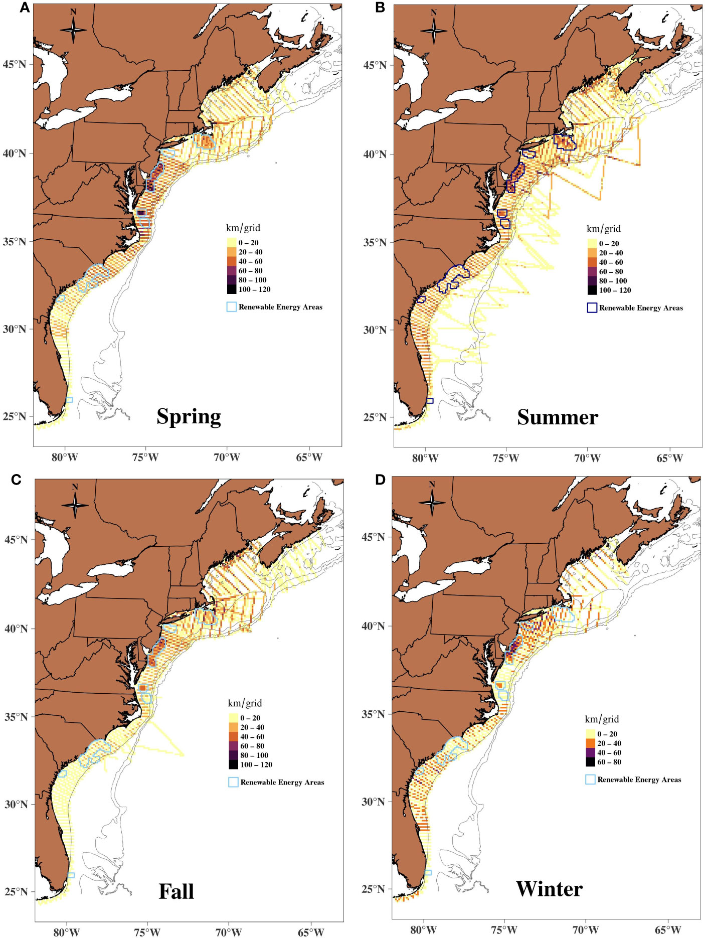
Figure 1 Seasonal coverage of the survey effort in the study area during 2010–2017 by the AMAPPS surveys. A) Spring, B) Summer, C) Fall and D) Winter. Most spatiotemporal grid were repeatedly surveyed.

Static and dynamic covariate characteristics of the environment within the study area were compiled from a variety of sources (Table 1). All line transect and environmental covariate data were subdivided into 10x10 km cells and 8-day time periods. In addition, average sea state and glare collected during the line transect surveys within each spatiotemporal cell was included as a continuous predictor variable, to account for sighting conditions encountered on the surveyed track lines.

TABLE 1

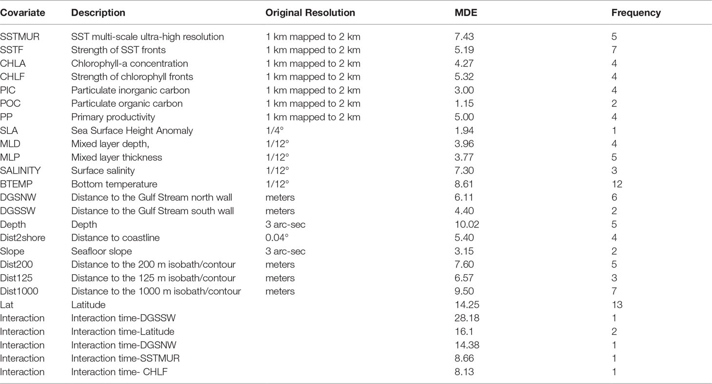
Table 1 Contemporaneous habitat covariates and interactions included in the habitat models; MDE is the mean deviance explained by a covariate when included in a model; Frequency is the number of models in which the covariate was included.

Analysis Methods

Two-step density surface modeling techniques were used to develop seasonal spatial models and maps of the density of the cetacean species (Miller et al., 2013) using the line transect sighting data collected during 2010 to 2017. The first step fits the detection functions to model the probability of observing animals away from the track line. The second step models the observed density estimated in the first step as a function of environmental covariate data and then uses the model to predict density over the entire survey area. The advantage of model-based techniques is the use of the additional environmental covariate data generally lead to more precise abundance estimates and the ability to predict abundance in regions in between the surveyed track lines. A key advantage of this technique is unbiased abundance estimates can be produced even when the data do not come from surveys designed to achieve equal coverage probability of the survey area (Hammond et al., 2021).

Mark-Recapture and Distance Analysis

The first step of the density surface modeling technique developed species-specific estimates of the line-transect detection probability parameters based on survey effort conducted in Beaufort Sea states from 0 through 4 (Palka, 1996; Barlow et al., 2001; Palka, 2012).

The density estimates were based on the independent observer approach assuming point independence (Laake and Borchers, 2004), calculated using mark-recapture distance sampling (MRDS) (Thomas et al., 2010), for each sampled spatiotemporal cell using a Horvitz-Thompson-like estimator (Borchers et al., 2006). With this approach, there was no need to independently model group size. To capture sightability differences between observation platforms and regions, data collected by each aircraft and ship from the SEFSC and NEFSC surveys were analyzed independently due to the differences in observers, data collection methods and habitats surveyed. Traditional MRDS distance analyses were used for the data collected by the shipboard surveys (Palka, 2020; Palka, 2012; Garrison, 2020). Data collected by the aerial surveys were analyzed using a two-step process as described by Palka et al. (2017) and Garrison (2020) to account for the slightly unbalanced area surveyed by the two teams in the planes.

Significant covariates were chosen following the method suggested by Marques & Buckland (2003) and Laake & Borchers (2004). For all of the analyses, the detection probabilities were estimated using right truncated perpendicular distances as suggested in Buckland et al. (2001) and model selection was based on the goodness-of-fit using the AIC score, Chi- squared test, Cramer-von Mises goodness-of-fit test and a visual inspection of the fit. The results of these test are available in Palka et al. (2021). The estimated sighting probability included an estimation of g(0) which is the probability of detecting an animal on the survey track line.

To ensure sufficient sample sizes to accurately estimate model parameters, when needed, several similar species were pooled. The criteria used to define species guilds included shape of the species’ detection functions, general animal behavior, perceived sightability of the species, and sample size. The estimated global parameters from the guild models were applied to the values of the covariates associated with each individual species in the guild to account for species-specific detection functions. An overall species-specific abundance estimate was then calculated for each spatiotemporal cell and corrected for species-specific availability bias by platform, as described in Palka et al. (2021); Palka et al. (2017).

Modeling Analysis

The second step in the density surface modeling technique developed a density habitat model. Generalized Additive Models (GAM) were developed in R (v. 4.1.1) using the package “mgcv” (v.1.8-36). Density estimates from the mark -recapture/distance analysis in sampled spatiotemporal cells were defined as the response variable in the generalized additive models. A habitat model was produced for each species to identify the extent of their habitat suitability over space and time. Potential habitat predictors included in the models consisted of a suite of 7 static physiographic characteristics in the study area and 14 contemporaneous dynamic environmental covariates (Table 1). The data sources are described in Palka et al. (2021).

The parameter estimates were optimized using restricted maximum likelihood criterion and the data were assumed to follow an overdispersed Tweedie distribution (Miller et al., 2013) with null space penalization and thin plate splines with shrinkage (Wood and Augustin, 2002). Further, to avoid overfitting that could render parameter estimates difficult to interpret biologically, the maximum number of degrees of freedom was limited to 5 and all models were checked to ensure this limit was appropriate. Correlations among environmental covariates ranged from 0.01–0.80 in absolute values. Although “mgcv” is considered to be robust to such correlations (Wood, 2011), both variables in a highly correlated pair were not used together in the same model.

Variable selection was performed with automatic term selection (Marra and Wood, 2011) and a suite of diagnostic tests as proposed by Kinlan et al. (2012) and Barlow et al. (2009). Models with the lowest prediction error and the highest percentage of deviance explained were selected for further testing which included k-fold cross-validation with 25 random data subsets.

Habitat Suitability Analysis

It was assumed that habitat suitability (HS), is directly correlated with the species’ abundance in relation to the unique combination of environmental predictors, as defined in Chavez-Rosales et al. (2019):

$HS={\displaystyle \sum _i^n}{\stackrel{⌢}{N}}_i$

where ${\widehat{N}}_i$is the estimated abundance from species-specific model for each spatiotemporal cell i. For this study the seasonal core habitat was defined as the area within a seasonal density map comprising of spatiotemporal cells with the upper 20% of predicted abundance values, based on the criteria defined in Hazen et al. (2012). Spring was defined from March to May, summer from June to August, fall from September to November and winter from December to February. Under this definition, the seasonal core habitat is meant to capture seasonal variability of the primary habitat used by each species. To determine if there were habitat shifts, we compared the core habitats for 2010 and 2017 in two ways. First, we compared the locations of the weighted centroids defined as the average coordinate of all points within the core habitat polygon weighted by the density estimates of the core habitat. Second, we compared the latitudinal distributions of the estimated abundance within the core habitat, which was calculated by summing the proportion of the estimated abundance within the core habitat by every 0.5-degree latitude.

Results

The 2010 – 2017 data were collected from over 250,000 km of on-effort line transect track lines from AMAPPS surveys (Table 2) resulting in the detection of 8,332 groups of cetaceans of over 110,068 individuals from 16 species (Supplementary Tables S1, S2). Approximately 68% of these groups were detected by the northern surveys. After the data processing, the final input data for the habitat models included 25,856 surveyed spatiotemporal cells for the 2010-2017 timeframe.

TABLE 2

Table 2 Seasonal effort in kilometers by platform from the AMAPPS surveys included in the analysis.

A total of 17 habitat models were developed that included data from all four seasons for most of the species. The exception was for species that inhabit only deeper shelf-edge waters that were only surveyed by the shipboard surveys during summer, such as Cuvier’s beaked whales and Sowerby’s beaked whales. In the case of harbor porpoise, two habitat models were developed to explain their distinct annual distribution patterns. One model included only data collected from months where the harbor porpoises were spatially clustered (June to October). The second model included data from months where the species was spatially spread out (November to May) (Supplementary Table S3; Supplementary Figures S1–S15).

The most frequent covariates included in the habitat models were latitude (13 models), bottom temperature (12 models), strength of the SST fronts (7 models), and distance to the 1000 m depth isobaths (7 models). Overall, the deviance explained by the habitat models ranged from 28% for bottlenose dolphin to 71% for striped dolphin. The models included between 3 to 9 habitat covariates, the mean contribution to the model by individual covariates ranged from 1.15% for particulate organic carbon to 28.18% for the interactions between time (8-day period for each year) and distance to the Gulf Stream south wall (Supplementary Table S3; Table 1). For all species, the average abundance estimates within the core habitat comprised 0.77 of the total abundance for 2010 and 2017. In 2010, the proportion of estimated abundance in the core habitat ranged from 0.55 for minke whale for fall to 0.98 for long-finned pilot whale during winter. In 2017, the proportion of estimated abundance in the core habitat ranged from 0.54 for minke whale for summer to 0.99 for long-finned pilot whale during fall (Supplementary Table S4). Comparisons of the weighted centroid for species-specific core habitat identified seasonal differences in patterns of habitat change for most species north of 34° latitude. The greatest shifts and magnitudes varied by season and species, but the shift tendency was towards the northeast (NE) (Figure 2). On average, fall showed the greatest shifts of the weighted centroid, with 168 km, followed by winter (134 km), spring (115 km) and summer (96 km). The largest shifts in the core habitat was for bottlenose dolphin, fin whale, short-finned pilot whale, Risso’s dolphin, sei whale, common dolphin, sperm whale and striped dolphin (Table 3).

FIGURE 2

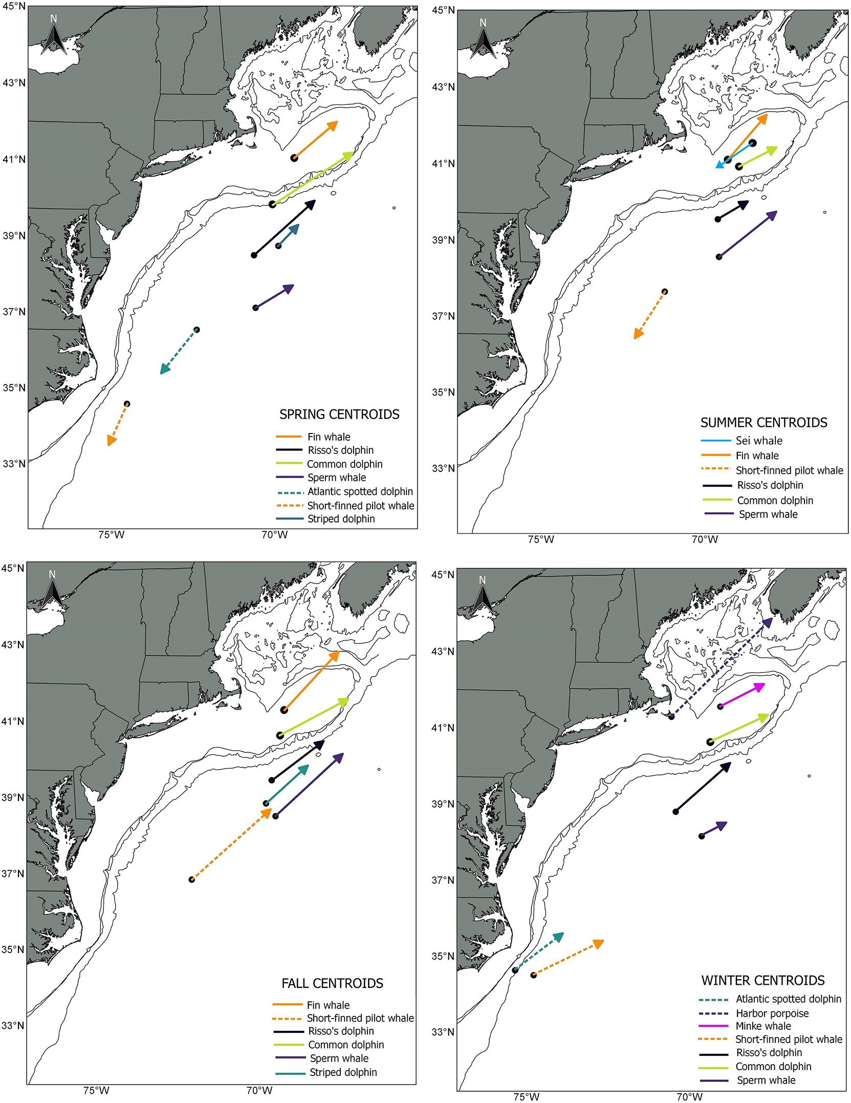
Figure 2 Direction and magnitude of core habitat shifts, represented by the length of the line of the seasonal weighted centroid for species with more than 70 km difference between 2010 (black dot) and 2017 (tip of arrow).

TABLE 3

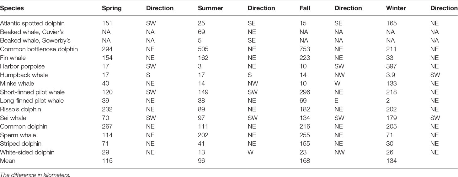
Table 3 Difference on the location of the core habitat weighted centroid (in km) and direction of the habitat shift between 2010 and 2017.

Overall, for species that showed a clear NE displacement of the weighted centroid, the average magnitude of the shift was 178 km. Bottlenose dolphin habitat showed the most drastic shift for all seasons except during winter: spring= 294 km, summer=505 km, fall= 753 km and winter = 211 (Table 3; Figures 3, 4). There was a clear tendency where the proportion of the estimated population in southern latitudes decreased, while north of 35° the proportion of the estimated population increased, especially during summer 2017 (Figure 5). Other species that on average, showed a moderate-to-no spatial shift included humpback whale, minke whale, white-sided dolphin, Sowerby’s beaked whale, and long-finned pilot whale (Table 3; Supplementary Figures S1 -S14).

FIGURE 3

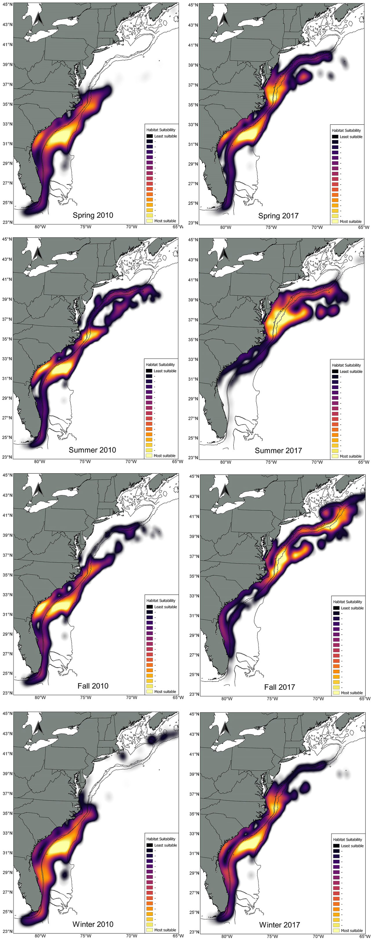
Figure 3 Difference in kilometers on the location of the core habitat weighted centroid and direction of the habitat shift between 2010 and 2017.

FIGURE 4

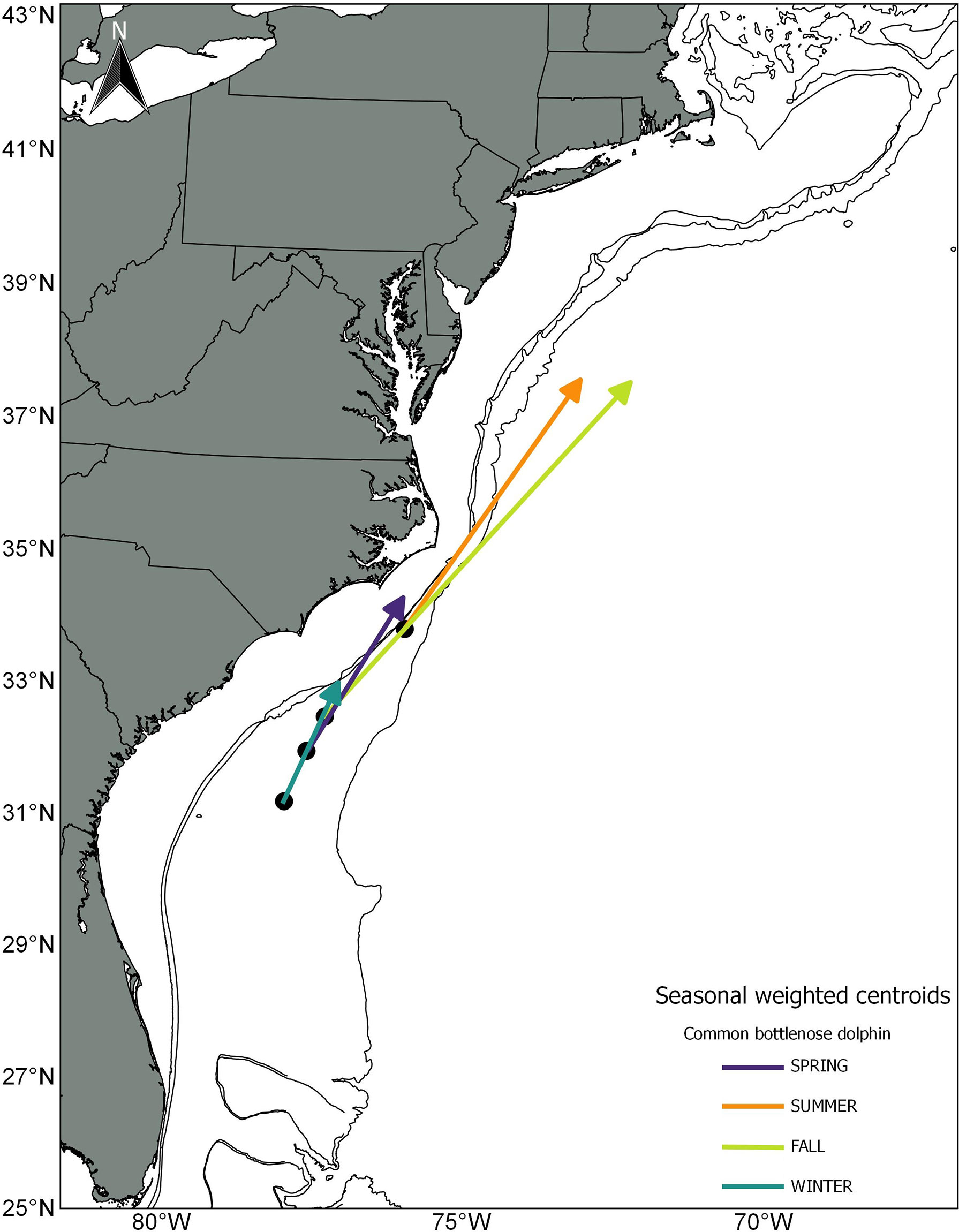
Figure 4 Direction and magnitude of core habitat shifts represented by the length of the line of the seasonal weighted centroid, for bottlenose dolphin between 2010 (black dot) and 2017 (tip of arrow).

FIGURE 5

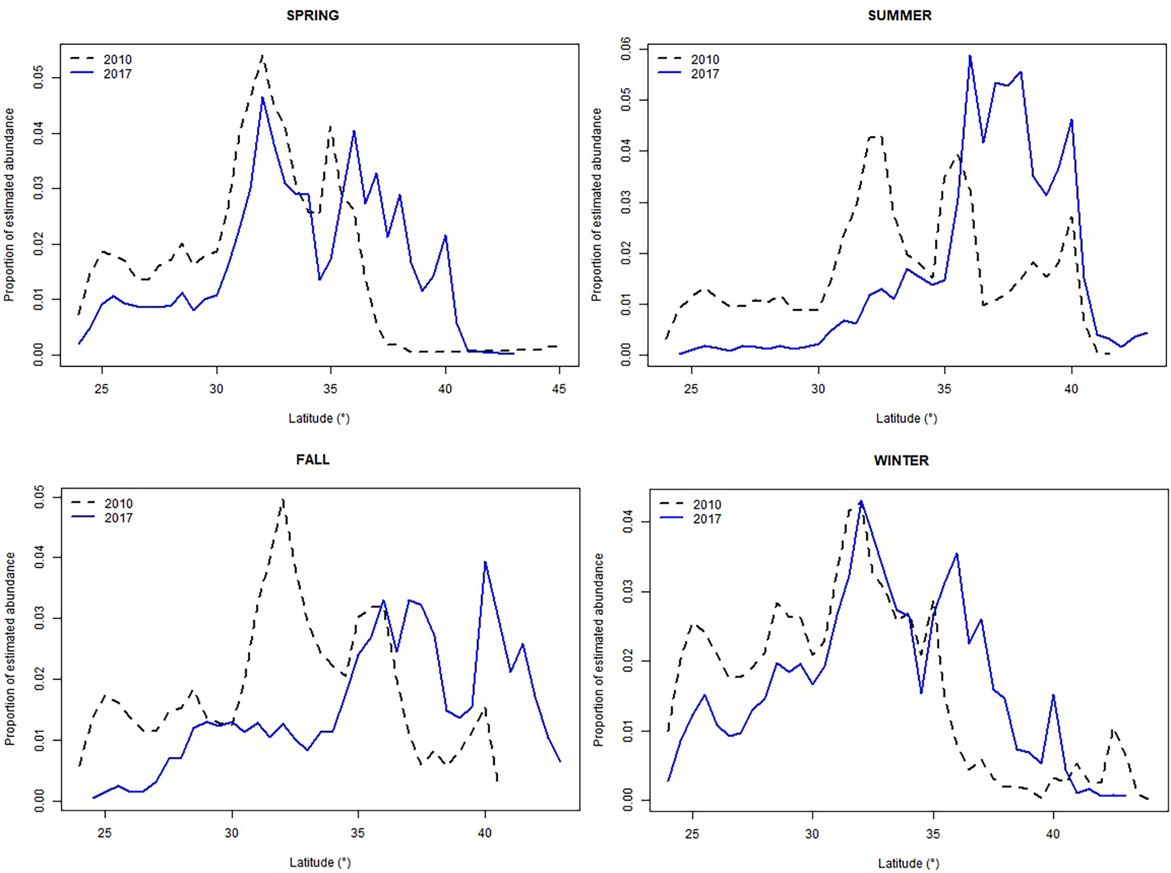
Figure 5 Seasonal comparison of the proportion of the estimated abundance within the core habitat for bottlenose dolphin by 0.5° latitudinal bins. 2010 dotted-black line, 2017 solid blue line.

Discussion

Climate change, most notably ocean warming is affecting the ecosystem in various ways leading to large and sometimes abrupt changes in the ecosystem’s structure. Those changes affect the interaction of multiple system covariates and can result in ecosystem reorganization (US NMFS NFSC, 2021). Previous studies used the premise of redistribution of marine organisms linked to their preferred thermal habitat, and several projections with future scenarios of species shifts were produced using coarse resolution global and earth climate models (Hobday et al., 2016; Tommasi et al., 2017). However, the difference in regional projections of climate change limit the confidence on the utility of those projections (Hawkins and Sutton, 2009; Frölicher et al., 2016). Our study explored a wider more expansive list of possible habitat predictors. We found bottom temperature and latitude more often correlated with the animal density, in comparison to SST or strength of SST fronts.

Latitude was the most common covariate included in the habitat density models. This covariate could be interpreted as denoting the general spatial patterns of a species distribution. Positive near-linear relationships between latitude and density were in the density-habitat models of the northern species usually found in waters north of North Carolina, about 37°N. In contrast, negative relationships were in the models for the southern species, such as the Atlantic spotted dolphins found mostly in waters south of New Jersey (about 40°N). The humpback whale’s model had a bimodal relationship with latitude that reflected its seasonal migration patterns up and down the coast. To model the large interannual variability in sei whale densities off the US coast, the most significant covariate was an interaction between latitude and time.

The second most common covariate included in the habitat density models was bottom temperature. Although SST and bottom temperature are somewhat related, the physical forcing factors for the two locations are different. It appears that bottom temperature was a good predictor of density for deep diving species, where this covariate could be interpreted to represent their prey preferences. The deepest divers that commonly feed at depths greater than 1500 m deep are the various beaked whales and Kogia sp. Their models indicated that high densities are in waters where the bottom temperature was below about 8°C. Other deep divers that commonly feed higher in the water column, at about 200 – 1000 m depth on species such as squid, appeared to be found in only a limited range of warmer bottom waters, such as about 7-17°C for sperm whales, pilot whales, Risso’s dolphins, common dolphins, bottlenose dolphins, and striped dolphins. The bottom temperature values with the higher than average densities of Atlantic spotted dolphins was bimodal, <6°C and >20°C, which appears to reflect the bimodal distribution of these animals off Florida and off Massachusetts.

Abiotic factors that are usually considered indicative of environmental (climate) changes include latitude, bottom temperature, SST, distance to the Gulf Stream. Biotic factors that could be indicative of organisms reacting to changing abiotic factors include primary productivity and chlorophyll a. These are the types of factors that were in the common bottlenose dolphin density-habitat model, which demonstrated dramatic seasonal shifts. The model covariates, in order of the contribution to the deviance explained, were interaction between SST and time, distance to the northern wall of the Gulf Stream, primary productivity, bottom temperature, bottom slope, chlorophyll a, and surface salinity.

Previous studies showed several limitations associated with statistical correlative models when used to extrapolate in time and areas where sampling effort was absent (Elith and Leathwick, 2009; Webber et al., 2011). For instance, the relationships implied from field data may not adequately describe factors determining species distributions, especially if the data are not collected consistently with a standardized protocol. Another limitation is large-scale environmental relationships developed from available data on past conditions, are generally considered less reliable to predict responses to extreme events or novel conditions under future climate changes (Hothorn et al., 2011; Williams et al., 2007).

This study uses data collected with standardized protocols from only the area of interest for the 2010-2017 time period. We also used high resolution contemporaneous values of the habitat covariates in the models to increase the confidence in the estimation of the habitat suitability. In addition, this study presumed a robust environmental multivariate nonlinear relationship with the distribution of cetacean species in the region (see Palka et al., 2021).

The tendencies on the cetacean habitat shifts identified in this paper are consistent with the shifts observed in fishing stocks within the same regions, which showed movement towards the northeastward and into deeper waters (US NMFS NFSC, 2021).

These species are primarily distributed in the Georges Bank and Gulf of Maine during summer and fall seasons. This study does not attempt to answer why they did not shift. However, perhaps it could be because all of these species typically inhabit the same areas, are considered prey generalists (as they can feed on a variety of prey ranging from krill to small schooling fish), and Northern sand lance (Ammodytes dubius) is known to be a key prey to all of these species (Weinrich et al., 2001; Craddock et al., 2009; Smith et al., 2015; Staudinger et al., 2020). As generalists they could be more adaptable to newly- available or changing prey species, if new prey species are arriving. Also, in this time and area since 2010 sand lance have probably been increasing because Atlantic herring (Clupea harengus) and Atlantic mackerel (Scomber scombrus) have been decreasing. Although scientists do not conduct assessments of Northern sand lance, this supposition is because the sand lance populations have been observed to oscillate out of phase with Atlantic herring and Atlantic mackerel (Staudinger et al., 2020; Suca et al., 2021), who have been decreasing since 2010 (Stock SMART 2021).

The results presented in this paper indicated the utility of using habitat models to estimate the core of habitat suitability. By including static and dynamic environmental covariates in the habitat models, these models provided an indicator of the seasonal and interannual variability and a good metric to detect habitat shifts and their magnitude. One important assumption of these models is the consistent statistical relationship within the spatiotemporal environment and the animal density (Chavez-Rosales et al., 2019). Based on this assumption, it is possible to interpolate the habitat preference of species in areas or periods of time within the study area and timeframe where surveys did not actually occur (Guisan et al., 2002). However, while these models are robust for the study area and timeframe, as indicated by the cross-validation analysis, the models are unable to directly detect changes in fundamental ecological processes such as predator-prey relationships through time and space. For this reason, in the future there is the need to incorporate more biological data related to possible prey availability into the habitat models formulation. Doing so would improve our understanding of the abundance and distribution of cetaceans in the region.

Habitat suitability estimated by specific habitat-based models such as those presented in this paper provide information to document past changes in the distribution and abundance of cetaceans as related to changes in their abiotic and biotic habitat. These past changes could then be used to predict potential future changes. Therefore, these habitat-based models have the potential to support management decisions related to the development of offshore regions for renewable energy and other activities and to promote conservation measures in a marine spatial planning context.

Data Availability Statement

The datasets presented in this study can be found in online repositories. The names of the repository/repositories and accession number(s) can be found below: https://github.com/NEFSC/READ-PSB-AMAPPS-public.

Author Contributions

DP and LG conceived the study, collected the cetacean survey data and assisted with the analyses. EJ processed survey and environmental data. S-CR conducted the analysis, prepared the figures and wrote the manuscript in collaboration with DP. All authors reviewed and edited the manuscript.

Funding

This study was funded by the US Department of Commerce, National Oceanic and Atmospheric Administration, National Marine Fisheries Services, by Interagency Agreements M14PG00005, M10G00075, and M19PG00007 between the US Department of Commerce, National Oceanic and Atmospheric Administration, National Marine Fisheries Services and the US Department of the Interior, Bureau of Ocean Energy Management, and by Interagency Agreements NEC-11-009, NEC-15-004, and NEC-16-011 between the US Department of Commerce, National Oceanic and Atmospheric Administration, National Marine Fisheries Services and the Department of the Navy, Office of the Chief of Naval Operations.

Conflict of Interest

SC-R and EJ are employed by Integrated Statistics in support of NOAA-Northeast Fisheries Science Center.

The remaining authors declare that the research was conducted in the absence of any commercial or financial relationships that could be construed as a potential conflict of interest.

Publisher’s Note

All claims expressed in this article are solely those of the authors and do not necessarily represent those of their affiliated organizations, or those of the publisher, the editors and the reviewers. Any product that may be evaluated in this article, or claim that may be made by its manufacturer, is not guaranteed or endorsed by the publisher.

Acknowledgments

We would like to thank the crews of the NOAA ships Henry B. Bigelow and Gordon Gunter and the NOAA Twin Otter aircrafts, all of the shipboard and aerial observers, and all the people involved in the data collection and analyses.

Supplementary Material

The Supplementary Material for this article can be found online at: https://www.frontiersin.org/articles/10.3389/fmars.2022.877580/full#supplementary-material

References

Barlow J., et al. (2009). Predictive Modeling of Cetacean Densities in the Eastern Pacific Ocean ( U.S. Department of Commerce, NOAA Technical Memorandum, NMFS-SWFSC-444), 206p. Available at: https://repository.library.noaa.gov/view/noaa/3666.

Google Scholar

Barlow J., Gerrodette T., Forcada J. (2001). Factors affecting perpendicular sighting distances on shipboard line-transect surveys for cetaceans. J. Cetacean. Res. Manage. 3, 201–212.

Google Scholar

Borchers D. L., Laake J. L., Southwell C., Paxton C. G. M. (2006). Accommodating Unmodeled Heterogeneity in Double-Observer Distance Sampling Surveys. Biometrics 62, 372–378. doi: 10.1111/j.1541-0420.2005.00493.x

PubMed Abstract | CrossRef Full Text | Google Scholar

Buckland S. T., Anderson D. R., Burnham K. P., Laake J. L., Borchers D., Thomas L. (2001). Introduction to Distance Sampling: Estimating Abundance of Biological Populations ( Oxford University Press).

Google Scholar

Chang, (2020). Shifting Habitats. Nat. Clim. Chang 10, 377. doi: 10.1038/s41558-020-0789-x

CrossRef Full Text | Google Scholar

Chavez-Rosales S., Palka D. L., Garrison L. P., Josephson E. A. (2019). Environmental Predictors of Habitat Suitability and Occurrence of Cetaceans in the Western North Atlantic Ocean. Sci. Rep. 9, 5833. doi: 10.1038/s41598-019-42288-6

PubMed Abstract | CrossRef Full Text | Google Scholar

Craddock J. E., Polloni P. T., Hayward B., Wenzel F. (2009). Food Habits of Atlantic White-Sided Dolphins (Lagenorhynchus Acutus) Off the Coast of New England. Fishery. Bull. 107 (3), 384–394.

Google Scholar

Elith J., Leathwick J. R. (2009). Species Distribution Models: Ecological Explanation and Prediction Across Space and Time. Ann. Rev. Ecol. Evol. Syst. 40, 677–697. doi: 10.1146/annurev.ecolsys.110308.120159

CrossRef Full Text | Google Scholar

Frölicher T. L., Rodgers K. B., Stock C. A., Cheung W. W. L. (2016). Sources of Uncertainties in 21st Century Projections of Potential Ocean Ecosystem Stressors. Global Biogeochem. Cycles 30, 1224–1243. doi: 10.1002/2015GB005338

CrossRef Full Text | Google Scholar

Garrison L. P. (2020). Abundance of Marine Mammals in Waters of the U.S. East Coast During Summer 2016 (75 Virginia Beach Conflict of Interest: Dr., Miami, FL: Southeast Fisheries Science Center, Protected Resources and Biodiversity Division), 17 pp.

Google Scholar

Goddard P. B., Yin J., Griÿes S. M., Zhang S. (2015). An Extreme Event of Sea-Level Rise Along the Northeast Coast of North America in 2009–2010. Nat. Commun. 2015, 6. doi: 10.1038/ncomms7346

CrossRef Full Text | Google Scholar

Guisan A., Edwards J. T. C., Hastie T. (2002). Generalized Linear and Generalized Additive Models in Studies of Species Distributions: Setting the Scene. Ecol. Model. 157, 89–100. doi: 10.1016/S0304-3800(02)00204-1

CrossRef Full Text | Google Scholar

Hammond P. S., Francis T. B., Heinemann D., Long K. J., Moore J. E., Punt A. E., Reeves R. R., Sepúlveda M., Sigurgsson G. M., Siple M. C., Víkingsson G., Wade P. R., Williams R., Zerbini A. N. (2021) Estimating the Abundance of Marine Mammal Populations. Front. Mar. Sci. 8:735770. doi: 10.3389/fmars.2021.735770

PubMed Abstract | CrossRef Full Text | Google Scholar

Hawkins E., Sutton R. (2009). The Potential to Narrow Uncertainty in Regional Climate Predictions. B. Am. Meteorol. Soc 90, 1095. doi: 10.1175/2009BAMS2607.1

CrossRef Full Text | Google Scholar

Hazen E., Jorgensen S., Rykaczewski R., Bograd S., Foley D., Jonsen I., et al. (2012). Predicted Habitat Shifts of Pacific Top Predators in a Changing Climate. Nat. Climate Change Lett. 6(3), 234–238. doi: 10.1038/NCLIMATE1686

CrossRef Full Text | Google Scholar

Hobday A. J., Alexander L. V., Perkins S. E., Smale D. A., Straub S. C., Oliver E. C. J., et al. (2016). A Hierarchical Approach to Defning Marine Heatwaves. Prog. Oceanography 141, 227–238. doi: 10.1016/j.pocean.2015.12.014

CrossRef Full Text | Google Scholar

Hothorn T., Muller J., Schroder B., Kneib T., Brandl R. (2011). Decomposing Environmental, Spatial, and Spatiotemporal Components of Species Distributions. Ecol. Monogr. 81, 329–347. doi: 10.1890/10-0602.1

CrossRef Full Text | Google Scholar

Kinlan B. P., Menza , C., Huettmann F. (2012). Chapter 6: Predictive Modeling of Seabird Distribution Patterns in the New York Bight. pp. 87-148. In: Menza C, Kinlan B.P, Dorfman D.S, Poti M., Caldow C(eds.). A Biogeographic Assessment of Seabirds, Deep Sea Corals and Ocean Habitats of the New York Bight: Science to Support Offshore Spatial Planning. NOAA Technical Memorandum NOS NCCOS 141. Silver Spring, MD. 224 pp. Available at: https://archive.org/details/BiogeographicAssessmentOfNewYorkBight

Google Scholar

Kleisner K. M., Fogarty M. J., McGee S., Barnett A., Fratantoni P., Greene J., et al. (2016). The Effects of Sub-Regional Climate Velocity on the Distribution and Spatial Extent of Marine Species Assemblages. PLos One, 11(2), 1–21. doi: 10.1371/journal.pone.0149220

CrossRef Full Text | Google Scholar

Laake J., Borchers D. (2004). Advanced Distance Sampling. Eds. Buckland S. T., Anderson D. R., Burnham K. P., Laake J. L., Thomas L. ( Oxford University Press), 108–189.

Google Scholar

Lavender E., Fox C., Borrows M. (2021). Modelling the Impacts of Climate Change on Thermal Habitat Suitability for Shallow-Water Marine Fish at a Global Scale. PLos One 16 (10), e0258184. doi: 10.1371/journal.pone.0258184

PubMed Abstract | CrossRef Full Text | Google Scholar

Marques F. C., Buckland S. T. (2003). Incorporating Covariates Into Standard Line Transect Analysis. Biometrics 59, 924–935. doi: 10.1111/j.0006-341X.2003.00107.x

PubMed Abstract | CrossRef Full Text | Google Scholar

Marra G., Wood S. (2011). Practical Variable Selection for Generalized Additive Models. Comput. Stat. Data Anal. 55, 2372–2387. doi: 10.1016/j.csda.2011.02.004

CrossRef Full Text | Google Scholar

Meynecke J., de Bie J., Barraqueta J., Seyboth E., Dey S., Lee S. B., et al. (2021). The Role of Environmental Drivers in Humpback Whale Distribution, Movement and Behavior: A Review. Front. Mar. Sci. 8. doi: 10.3389/fmars.2021.720774

PubMed Abstract | CrossRef Full Text | Google Scholar

Miller D. L., Burt M. L., Rexstad E. A., Thomas L., Gimenez O. (2013). Spatial Models for Distance Sampling Data: Recent Developments and Future Directions. Methods Ecol. Evol. 4, 1001–1010. doi: 10.1111/2041-210X.12105

CrossRef Full Text | Google Scholar

Morley J. W., Selden R. L., Latour R. J., Frölicher T. L., Seagraves R. J., Pinsky M. L. (2018). Projecting Shifts in Thermal Habitat for 686 Species on the North American Continental Shelf. PLos One 13, e0196127. doi: 10.1371/journal.pone.0196127

PubMed Abstract | CrossRef Full Text | Google Scholar

Palka D. (1996). Effects of Beaufort Sea State on the Sightability of Harbor Porpoises in the Gulf of Maine. Rep. Int. Whal. Commn. 46, 575–582.

Google Scholar

Palka D. (2012). Cetacean Abundance Estimates in US Northwestern Atlantic Ocean Waters From Summer 2011 Line Transect Survey ( US Dept Commer), 37 p. Available at: https://repository.library.noaa.gov/view/noaa/4312. National Marine Fisheries Service, 166 Water Street, Woods Hole, MA 02543-1026.

Google Scholar

Palka D. (2020). Cetacean Abundance in the US Northwestern Atlantic Ocean Summer 2016 ( US Dept Commer), 60 p. Available at: https://apps-nefsc.fisheries.noaa.gov/rcb/publications/crd2005.pdf.

Google Scholar

Palka D., Aichinger Dias L., Broughton E., Chavez-Rosales S., Cholewiak D., Davis G., et al. (2021). Atlantic Marine Assessment Program for Protected Species: FY15 – Fy19 (Washington DC: US Department of the Interior, Bureau of Ocean Energy Management), 330 p. Available at: https://marinecadastre.gov/espis/#/search/study/100066. OCS Study BOEM 2021-051.

Google Scholar

Palka D. L., Chavez-Rosales S., Josephson E., Cholewiak D., Haas H. L., Garrison L., et al. (2017). Atlantic Marine Assessment Program for Protected Species (Washington, DC: US Dept. of the Interior, Bureau of Ocean Energy Management, Atlantic OCS Region), 211 pp.

Google Scholar

Patel S., Winton M., Hatch J., Hass H., Saba V., Fay G., et al. (2021). Projected Shifts in Loggerhead Sea Turtle Thermal Habitat in the Northwest Atlantic Ocean Due to Climate Change. Sci. Rep. 11, 8850. doi: 10.1038/s41598-021-88290-9

PubMed Abstract | CrossRef Full Text | Google Scholar

Pinsky M. L., Worm B., Fogarty M. J., Sarmiento J. L., Levin S. A. (2013). Marine Taxa Track Local Climate Velocities. Science 341, 1239–1242. doi: 10.1126/science.1239352

PubMed Abstract | CrossRef Full Text | Google Scholar

Pinsky M. L., Selden R. L, Kitchel Z. J. and . (2020) Climate-driven shifts in marine species ranges: scaling from organisms to communities. Annu. Rev. Mar. Sci. 12:153–79. doi: 10.1146/annurev-marine-010419-010916

CrossRef Full Text | Google Scholar

Smith L. A., Link J. S., Cadrin S. X., Palka D. L. (2015). Consumption by Marine Mammals on the Northeast US Continental Shelf. Ecol. Appl. 25 (2), 373–389. doi: 10.1890/13-1656.1

PubMed Abstract | CrossRef Full Text | Google Scholar

Staudinger M. D., Goyert H., Suca J. J., Coleman K., Welch L., Llopiz J. K., et al. (2020). The Role of Sand Lances (Ammodytes Sp.) in the Northwest Atlantic Ecosystem: A Synthesis of Current Knowledge With Implications for Conservation and Management. Fish. Fisheries 31 (3), 522–556. doi: 10.1111/faf.12445

CrossRef Full Text | Google Scholar

Suca J. J., Wiley D. N., Silva T. L., Robuck A. R., Richardson D. E., Clancy S. G., et al. (2021). Sensitivity of Sand Lance to Shifting Prey and Hydrography Indicates Forthcoming Change to the Northeast US Shelf Forage Fish Complex. ICES. J. Mar. Sci. 78 (3), 1023–1037. doi: 10.1093/icesjms/fsaa251

CrossRef Full Text | Google Scholar

Thomas L., Buckland S. T., Rexstad E. A., Laake J. L., Strindberg S., Hedley S. L., et al. (2010). Distance Software: Design and Analysis of Distance Sampling Surveys for Estimating Population Size. J. Appl. Ecol. 47, 5–14. doi: 10.1111/j.1365-2664.2009.01737.x

PubMed Abstract | CrossRef Full Text | Google Scholar

Tommasi D., Stock C. A., Pegion K., Vecchi G. A., Methot R. D., Alexander M. A., et al. (2017). Improved Management of Small Pelagic Fisheries Through Seasonal Climate Prediction. Ecol. Appl. 27, 378–388. doi: 10.1002/eap.1458

PubMed Abstract | CrossRef Full Text | Google Scholar

US NMFS NFSC (2021). “State of the Ecosystem 2021,” in New England Revised, 43 p. doi: 10.25923/6pww-mw45

CrossRef Full Text | Google Scholar

Van Weelen C., Towers J. R., Bosker T. (2021). Impacts of Climate Change on Cetacean Distribution, Habitat and Migration. Climate Change Ecol. 1, 100009. doi: 10.1016/j.ecochg.2021.100009

CrossRef Full Text | Google Scholar

Webber B. L., Yates C. J., Le Maitre D. C., Scott J. K., Kriticos D. J., Ota N., et al. (2011). Modelling Horses for Novel Climate Courses: Insights From Projecting Potential Distributions of Native and Alien Australian Acacias With Correlative and Mechanistic Models. Div. Distrib. 17, 978–1000. doi: 10.1111/j.1472-4642.2011.00811.x

CrossRef Full Text | Google Scholar

Weinrich M. T., Belt C. R., Morin D. (2001). Behavior and Ecology of the Atlantic White-Sided Dolphin (Lagenorhynchus Acutus) in Coastal New England Waters. Mar. Mammal Sci. 17 (2), 231–248. doi: 10.1111/j.1748-7692.2001.tb01268.x

CrossRef Full Text | Google Scholar

Williams J. W., Jackson S. T., Kutzbach J. E. (2007). Projected Distributions of Novel and Disappearing Climates by 2100 AD. Proc. Natl. Acad. Sci. U.S.A. 104, 5738–5742. doi: 10.1073/pnas.0606292104

PubMed Abstract | CrossRef Full Text | Google Scholar

Wood S. N. (2011). Fast Stable Restricted Maximum Likelihood and Marginal Likelihood Estimation of Semiparametric Generalized Linear Models. J. R. Stat. Soc Ser. B 73, 3–36. doi: 10.1111/j.1467-9868.2010.00749.x

CrossRef Full Text | Google Scholar

Wood S. N., Augustin N. H. (2002). GAMs With Integrated Model Selection Using Penalized Regression Splines and Applications to Environmental Modeling. Ecol. Model. 157, 157–177. doi: 10.1016/S0304-3800(02)00193-X

CrossRef Full Text | Google Scholar