 Ivan H. Y. Kwong
 Frankie K. K. Wong
 Tung Fung1,2
- 1Department of Geography and Resource Management, The Chinese University of Hong Kong, Hong Kong, Hong Kong SAR, China
- 2Institute of Future Cities, The Chinese University of Hong Kong, Hong Kong, Hong Kong SAR, China
Continuous monitoring of coastal water qualities is critical for water resource management and marine ecosystem sustainability. While remote sensing data such as Sentinel-2 satellite imagery routinely provide high-resolution observations for time-series analysis, the cloud-based Google Earth Engine (GEE) platform supports simple image retrieval and large-scale processing. Using coastal waters of Hong Kong as the study area, this study utilized GEE to (i) query and pre-process all Sentinel-2 observations that coincided with in situ measurements; (ii) extract the spectra to develop empirical models for water quality parameters using artificial neural networks; and (iii) visualize the results using spatial distribution maps, time-series charts and an online application. The modeling workflow was applied to 22 water quality parameters and the results suggested the potential to predict the levels of several nutrients and inorganic constituents. In-depth analyses were conducted for chlorophyll-a, suspended solids and turbidity which produced high correlations between the predicted and observed values when validated with an independent dataset. The selected input variables followed spectral characteristics of the optical constituents. The results were considered more robust compared to previous works in the same region due to the automatic extraction of all available images and larger number of observations from different years and months. Besides visualizing long-term spatial and temporal variabilities through distribution maps and time-series charts, potential anomalies in the monitoring period including algal bloom could also be captured using the models developed from historical data. An online application was created to allow novice users to explore and analyze water quality trends with a simple web interface. The integrated use of remotely-sensed images, in situ measurements and cloud computing can offer new opportunities for implementing effective monitoring programs and understanding water quality dynamics. Although the obtained levels of accuracies were below the desired standard, the end-to-end cloud computing workflow demonstrated in this study should be further investigated considering the cost and computational efficiency for timely information delivery.
Introduction
Water quality has gradually experienced degradation in many coastal regions because of pollution and heavy use resulting from anthropogenic activities (Chen et al., 2004; Gholizadeh et al., 2016). In Hong Kong, the Harbour Area Treatment Scheme has been commenced since 2001 to improve the water quality of Victoria Harbour at a cost of US$ 2.5 billion (Xu et al., 2011). Nevertheless, the marine environment of Hong Kong is still under considerable pressure from local, regional and global stressors such as reclamation, overfishing, biological invasion, transboundary pollution and climate change (Lai et al., 2016). Continuous monitoring and assessment of the water quality are critical for water resource management and marine ecosystem sustainability.
Water quality can be considered as a general descriptor of water properties in terms of physical, chemical and biological characteristics (Ritchie et al., 2003). Many water quality parameters, such as chlorophyll-a (Chl-a), suspended solids (SS), and turbidity, have been commonly used as indicators (Hafeez et al., 2019; Topp et al., 2020). For instance, Chl-a is a photosynthetic pigment and can be used as indirect measurements of phytoplankton biomass, algal production and trophic state (Schalles, 2006; Flores-Anderson et al., 2020). Rapid growth of algae or cyanobacteria can lead to harmful algal blooms that adversely affect people and ecology (Poddar et al., 2019; Wang et al., 2020). SS refers to both inorganic and organic particles held in suspension throughout a water column (Topp et al., 2020). Their movements are related to sediment transport, nutrient cycle and water clarity and are often linked to economic activities in ports and waterways (Shahzad et al., 2018; Wang et al., 2018). Turbidity is closely related to SS and is a measurement of light scattering within a water column caused by particles (Matthews, 2011). Increasing turbidity can reduce light penetration and cause cloudiness of the water (Khan et al., 2021).
Traditionally, water samples are collected from the field and then analyzed in the laboratory. Although such in situ measurements offer high accuracy, they are costly, labor-intensive and time-consuming (Gholizadeh et al., 2016; Pizani et al., 2020). Spatial and temporal variations within the entire waterbody are also hard to be identified from the sampling points (Ouma et al., 2020). On the other hand, recent advances in remote sensing technology have enabled the extraction of spatial and temporal profiles of surface water by providing a synoptic and synchronized view from aerial or satellite platforms over a large area (Schaeffer et al., 2013; Ansper and Alikas, 2019; Flores-Anderson et al., 2020). Since the upwelling radiance from the water at various wavelengths often consists of signals from the optically active components of the water (Ritchie et al., 2003; Shahzad et al., 2018), the spectral shapes and magnitudes of the water-leaving reflectance can be used directly or indirectly to detect different water quality parameters through empirical or analytical models (Matthews, 2011; Salem et al., 2017; Wang and Yang, 2019).
Despite a large amount of satellite data being available for remote sensing of water quality, only a few satellites can provide sufficient spatial, spectral and temporal resolutions to resolve the complex water variability in coastal areas. Ocean color sensors specifically designed for marine purposes (e.g., SeaWiFS, MODIS, MERIS) (Hu et al., 2012) cannot fulfil the requirements of coastal water monitoring due to their coarse spatial resolutions (> 250 m) (Mouw et al., 2015). Land sensors with moderate resolutions, especially the Landsat series satellites (30 m), were found to be the most popular data resources, mainly because of their temporal coverage and easy accessibility (Wang and Yang, 2019). Still, the revisit time of Landsat-8 (16 days) limits its use in routine monitoring of water quality (Toming et al., 2016).
Currently, the Multispectral Instrument (MSI) onboard Sentinel-2, launched by the European Space Agency Copernicus program in 2015, has opened a new potential in water remote sensing (Drusch et al., 2012). The MSI sensor measures radiance in 13 spectral bands spanning from visible to shortwave infrared with 10–60 m spatial resolution, including three red-edge bands that can be advantageous over optically complex coastal waters (Pahlevan et al., 2017; Ansper and Alikas, 2019), and provides a 5-day revisit frequency with both Sentinel-2A and Sentinel-2B satellites (Toming et al., 2016). In particular geographical areas like Hong Kong which are located at the edge of the sensor swath, Sentinel-2 is also preferred over Landsat satellites since its wider swath width can provide complete coverage of the study area in a single scene.
Images obtained from Sentinel-2 MSI have been demonstrated to successfully derive water quality parameters in a variety of scenarios, such as inland water reservoirs (Ouma et al., 2020; Pizani et al., 2020; Pompêo et al., 2021), lakes (Liu et al., 2017; Ansper and Alikas, 2019; Free et al., 2020; Soomets et al., 2020), rivers (Kuhn et al., 2019), estuaries (Sent et al., 2021) and bays with aquaculture (Gernez et al., 2017; Soriano-González et al., 2019). However, most of these analyses focused on the development of algorithms and only utilized images acquired from a single date or a limited temporal range (Topp et al., 2020). The strength of remote sensing lies in providing both comprehensive historical records of water quality, which facilitates understanding of long-term environmental changes (Kim et al., 2020), and near real-time measurement at critical points, where in situ measurements are not readily available (Sobel et al., 2020). Considering that Sentinel-2 data will be available routinely for many years and free of charge, several studies also emphasized the importance of using multi-temporal images to provide time-series analysis of changes and trends (Toming et al., 2016; Tamiminia et al., 2020; Elhag et al., 2021).
When utilizing satellite images for routine monitoring of water quality parameters, researchers have argued that computational demands required for managing and analyzing large volumes of data can be a major bottleneck (Kumar and Mutanga, 2018; Page et al., 2019). Compared to conventional image processing techniques, Google Earth Engine (GEE), a cloud-based platform for large-scale geospatial analysis (Gorelick et al., 2017), has been demonstrated to provide easy accessibility to readily available data and powerful computing capabilities for a variety of applications (Traganos et al., 2018; Tamiminia et al., 2020; Jia et al., 2021; Li et al., 2021). However, only a few studies have attempted to exploit the functionality of GEE to develop an automated approach or even a web application that can further enhance usability of the outputs (Markert et al., 2018; Rudiyanto et al., 2019; Canty et al., 2020). Hence, this study aimed to fill the gap by developing a low-cost, end-to-end and efficient workflow that can provide rapid information for improving water quality monitoring.
Among the previous remote sensing-based studies of water quality in Hong Kong, Wong et al. (2007; 2008) used MODIS images to retrieve Chl-a, SS and turbidity for coastal waters of Hong Kong, but the coarse spatial resolution (500 m) limited their usability in the spatially complex environment. Tian et al. (2014) produced the first map of SS concentration at moderate spatial resolution (30 m) in the Deep Bay area of Hong Kong using HJ-1 satellite images, despite the fact that their study focused only on a narrow range of SS concentrations and a specific area inside Hong Kong. Nazeer and Nichol (2015) developed an empirical model for estimation of SS concentrations by combining Landsat-5, Landsat-7 and HJ-1 images, although they are old-generation satellites with less desirable band designations and data bit levels. A recent study by Hafeez et al. (2019) focused on the comparison of several machine learning techniques for improving water quality estimation with Landsat series satellites, while Hafeez and Wong (2019) tested the performance of using Sentinel-2 images to estimate Chl-a and SS in a single year. These studies were either limited to using few image dates and in situ samples for model development and validation, or not providing a solution to operational water monitoring in different scenarios.
The objective of this study was to develop an automated framework to retrieve the spatial and temporal patterns of different water quality parameters, specifically Chl-a, SS and turbidity, for coastal waters of Hong Kong by integrating Sentinel-2 image time-series, in situ measurements from monitoring stations and the GEE cloud computing capability. In particular, this study aimed to utilize GEE to (i) query and pre-process all Sentinel-2 observations that coincided with in situ measurements; (ii) extract the spectra to develop empirical models for water quality parameters using artificial neural networks (ANN); and (iii) visualize the results using spatial distribution maps, time-series charts and an online application. The first part of this study presents the processing workflow and demonstrates that it could be applied to all 22 water quality parameters collected by monitoring stations. The second part of this study focuses on the modeling results of three major water quality parameters, including Chl-a, SS and turbidity. Through evaluating the empirical modeling performance and analyzing the water quality changes, this study provided both theoretical and practical implications, facilitating the implementation of an effective water resource monitoring program.
Materials and Methods
Study Area
Hong Kong is a highly urbanized city lying at the northern limits of the Asian tropics between latitudes 22°08’N and 22°35’N and longitudes 113°49’E and 114°31’E (Figure 1). The climate is subtropical, with hot rainy summers from May to August and cool dry winters from November to March. Situated with the Pearl River Estuary to the west and surrounded by the South China Sea to the south and east, Hong Kong has a land area of 1,108 km2 including more than 250 offshore islands. The coastline extends around 1,200 km and the sea area is 1,648 km2. The marine waters support diverse forms of marine life ranging from microscopic algae to dolphins, and are used for navigation, recreation, seafood production, and supply of flushing and cooling water (Environmental Protection Department, 2021).

Figure 1 (A) The study area of this study, including the 10 water control zones defined by the Environmental Protection Department (EPD) of the Hong Kong government; (B) Location of Hong Kong in the regional context.
Due to the combination of anthropogenic activities and variable hydrographical conditions, the coastal waters of Hong Kong are physically and chemically complex (Hafeez et al., 2019). For example, in the western areas (e.g. Deep Bay and North Western Zones), estuarine waters are influenced by freshwater discharge from the Pearl River. Water quality in this area is also influenced by the sediment loads and nutrients in the river discharges (Zhou et al., 2007). Conversely, the eastern waters (e.g. Mirs Bay) are more oceanic and influenced by the Pacific currents (Lai et al., 2016). The central areas represent a transition zone that varies seasonally, in addition to the influence of local pollution load from Victoria Harbour (Xu et al., 2011). The water quality also varies spatiotemporally depending on two seasonal monsoons. While the northeast monsoon prevails and enhances the effect of China Coastal Current during winter, the southwest monsoon in summer transports continental shelf water landward (Zhou et al., 2012). The estuarine plume covers the northern part of South China Sea when the river discharge is large in summer. The normal tidal range in Hong Kong waters is between one and two meters, with flood tide for oceanic water to flow to the northwestern direction and ebb tide in the reversed direction.
Water Quality Parameters and Station-Based Data
The Environmental Protection Department (EPD) of the Hong Kong government has divided Hong Kong waters into 10 water control zones (Figure 1) based on the hydrodynamic characteristics and pollution status. A systematic marine water quality monitoring program has been in operation since 1986 to measure a total of 22 water quality parameters (Environmental Protection Department, 2021). The list of the measured parameters is shown in Table 1, and they are related to different aspects of water quality including (i) physical and aggregate properties, (ii) aggregate organic constituents, (iii) nutrients and inorganic constituents, and (iv) biological and microbiological examination. The modeling workflow was applied to all 22 parameters in the first part of the present study, while detailed analyses focused on three major parameters, including Chl-a, SS and turbidity.
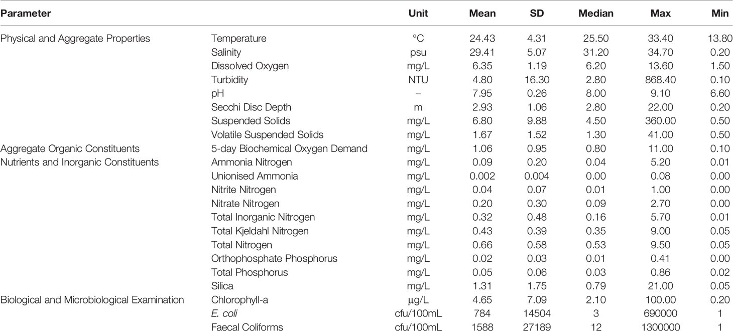
Table 1 Summary statistics of station-based monitoring data of the water quality parameters extracted in this study.
EPD takes measurements and collects water samples at 76 monitoring stations in open waters every month using their dedicated marine monitoring vessel equipped with Differential Global Positioning Systems (DGPS) and an advanced conductivity-temperature-depth (CTD) profiler. The water quality parameters are measured from three depths, including surface water (1 m below the sea surface), middle water (half the sea depth), and bottom water (1 m above the seabed). Water samples are collected in a 500 mL Nalgene bottle and analyzed by EPD’s in-house laboratory. To measure Chl-a concentration (µg/L), the American Public Health Association (APHA) 20ed 10200H2 spectrophotometric method based in-house GL-OR-34 method is used. For SS concentration (mg/L), the APHA 22ed 2540D weighing method based in-house GL-PH-23 method is used, while turbidity (NTU) is measured on-site by the OBS-3 turbidity sensor linked to a SEACAT 19+ CTD and Water Quality Profiler.
The marine water quality monitoring data are open data in the Hong Kong government online database (https://data.gov.hk/). The data are updated yearly and released usually in the third quarter of the next year. In this study, we retrieved the water quality data from 2015 to 2020 which match the availability of Sentinel-2 images. While this study was conducted in late 2021, station-based data covering the current year were not yet available. A summary of the station-based data is provided in Table 1.
Selection and Pre-Processing of Sentinel-2 Images
Sentinel-2 is an Earth observation mission from the Copernicus Program and consists of two identical satellites. Sentinel-2A was launched on 23rd June 2015 and Sentinel-2B was launched on 7th March 2017. The band configuration of Sentinel-2 is given in Table 2. The bands range from 443 nm to 2190 nm, featuring four bands at 10-m (Visible and near-infrared [NIR]), six bands at 20-m (red-edge and shortwave infrared [SWIR]) and three bands at 60-m (atmospheric) spatial resolution.
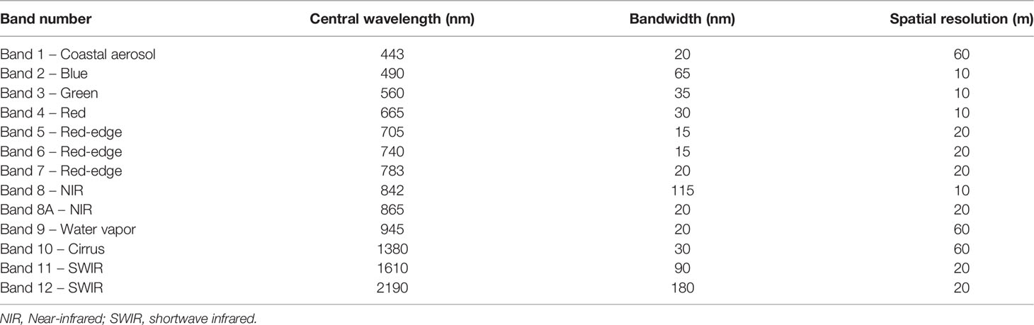
Table 2 Spectral bands for Sentinel-2 sensors (Drusch et al., 2012). Bands 8, 9 and 10 were eliminated in this study due to the wavelength overlap or absence of water surface information.
In this study, selection of suitable Sentinel-2 images and subsequent pre-processing steps were done using GEE (https://code.earthengine.google.com/). GEE includes both a web-based Code Editor in JavaScript language and a Python application programming interface (API) for data analysis outside the web environment (Tamiminia et al., 2020). All the analysis procedures in this study were written using GEE Python API in Google Colab (https://colab.research.google.com/) such that the codes can be directly executed through a web browser with minimal configuration.
The complete archive of Sentinel-2 images (Level-1C) from 2015 is available as an image collection in the GEE repository. Despite the ready availability of atmospherically corrected Level-2A products, this collection only contains images dating back to 2017, which makes it less suitable for time-series analysis. Instead, Level-1C images covering the study area were queried in GEE with a maximum cloudy pixel percentage of 20% according to metadata. A total of 120 cloud-limited scenes from 23rd October 2015 to 31st December 2021, covering all seasons of the year, were retrieved and used in this study (Table 3).
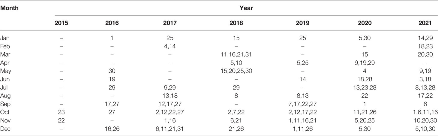
Table 3 Dates of the cloud-limited Sentinel-2 scenes retrieved and analyzed in this study.
The Level-1C Sentinel-2 data contained spectral values representing the top of atmosphere (TOA) reflectance. Atmospheric correction is an important process to obtain water-leaving reflectance by removing atmospheric interference from the total signal received by the satellite sensor (Soriano-González et al., 2019). This study implemented an atmospheric correction model called Py6S (Wilson, 2013), which is a Python interface of the “Second Simulation of the Satellite Signal in the Solar Spectrum” (6S) radiative transfer model (Vermote et al., 1997), to all Sentinel-2 images with the maritime aerosol setting. Py6S was chosen since it was found to be the best method over complex coastal waters of Hong Kong when tested using satellite images with similar resolutions (Nazeer et al., 2014) and relevant codes have been developed for GEE (Murphy, 2020).
For each atmospherically corrected image, a cloud mask was applied based on the s2cloudless dataset, which is a machine learning-based cloud detector precomputed on GEE (Zupanc, 2017). Cloud shadows were also estimated and masked using the position of detected clouds and the viewing geometry. Since some of the images were found to be affected by sun glints, a simple correction method was applied by subtracting 50% of the reflectance values of band 11 (SWIR) in each pixel from all bands. It was based on the assumption that the water-leaving radiance in SWIR wavelength is very low, thus a significant proportion of the SWIR signals that appear on the image could be attributed to sun glints and these signals correlate well with the glints experienced by other channels (Kay et al., 2009). The value was selected with reference to previous analysis of surface reflectance (Kuhn et al., 2019) and manual inspection of images acquired in adjacent swath with different viewing angles. In addition, the Modified Normalized Difference Water Index (MNDWI) for open waters (Xu, 2006), calculated as the difference-sum ratio of SWIR and visible green bands, was applied to all images to separate water pixels from land areas and remove low-quality pixels with a threshold value of zero.
Among the 13 spectral bands acquired by Sentinel-2, bands 9 (water vapor) and 10 (cirrus) were eliminated as they do not contain water surface information. Band 8 (NIR) was also removed since its wavelength overlaps with band 8A and the latter band provides more precise spectral measurement. The pre-processed images contained 10 spectral bands ranging from visible and NIR to SWIR wavelengths. The difference in spatial resolutions among spectral bands was not an issue in GEE which uses scale specified by the output to determine the appropriate level of input image pyramids.
Development of Empirical Models
Sentinel-2 reflectance values were extracted from the location of in situ measurements with an allowance of one-day difference, to ensure sufficient match-up points and consider the short water residence time of around two days in the wet season (Zhou et al., 2012). A 20-m buffer was adopted for each sampling point to reduce the effects of positional accuracy and noise from the sensor. All sampling locations were at least 200 m away from land to reduce adjacency effects. Furthermore, low-quality points were removed by Tukey’s fences method, which considered the point as an outlier if the value in any one of the spectral bands exceeded a distance of “1.5 times interquartile range” below the first or above the third quartiles. This resulted in a total of 352 observations, for which 300 observations in 2015–2019 were used for training and model development, while the remaining 52 observations in 2020 were used for validation, in order to demonstrate the model performance to estimate current water qualities from historical data.
Many algorithms have been proposed for retrieving water quality parameters from remote sensing reflectance. Among them, empirical methods aim to establish the relationships using statistical techniques and have advantages of computational simplicity and ease of implementation for different water quality parameters (Ritchie et al., 2003; Wang and Yang, 2019). A locally optimized algorithm is often recommended to provide better performances when calibrated with in situ observations (Tian et al., 2014; Yoon et al., 2019; Flores-Anderson et al., 2020). To establish a suitable model in this study, the following band ratios and arithmetic variables, which were developed with reference to bio-optical properties of waters (Matthews, 2011), were computed as input predictors.
Two-band ratios—The use of band ratios theoretically reduces the effects of tidal or seasonal variations and maximizes the sensitivity to water quality parameters against other constituents (Gons, 1999). For instance, a blue-green ratio uses the strong light absorption by carotenoids at 490 nm (blue) and minimal absorption of photosynthetic pigments at 560 nm (green). The ratio between 705 nm and 665 nm spectra is also based on the interaction between backscattering from particulate matter and the absorption features (Toming et al., 2016). Since there is little consistency in the optimal band ratios in different studies (Matthews, 2011), possible ratio combinations of all 10 spectral bands were computed and tested in this study. Instead of simple ratios, normalized band ratios were adopted in this study in order to limit the range between -1 and 1 (Equation 1).
Where i and j are any bands from 1 to 12 except 9 and 10, R(i) represents the reflectance of band i.
Three-band ratio—The three-band method was developed by Dall’Olmo and Gitelson (2005) with a basic principle to find the three-band combinations that are most relevant to the absorption coefficient of the water quality parameters (Wang and Yang, 2019). A typical example is the use of 665-nm, 705-nm and 740-nm wavelengths, which showed good agreement with in situ Chl-a data in turbid and productive waters (Ansper and Alikas, 2019). In this study, all possible combinations from three consecutive bands were calculated according to Equation 2.
Where i, j and k are any three consecutive bands from 1 to 12 except 9 and 10, R(i) represents the reflectance of band i.
Line-height variable—The line-height algorithm is based on band differences and measures the height of a reflectance peak at a specific wavelength from a linear baseline drawn between two sides of the peak (Gitelson et al., 1994). The fluorescence line height algorithm (Gower et al., 1999) and maximum chlorophyll index (Gower et al., 2005) are examples developed using the peaks of different MERIS bands related to Chl-a concentrations. To test the applicability of various choices of peak wavelengths, line-height variables were computed in this study from each of the 10 Sentinel-2 spectral bands with the adjacent two bands (Equation 3).
Where i, j and k are any three consecutive bands from 1 to 12 except 9 and 10, R(i) represents the reflectance of band i, λ(i) represents the central wavelength of band i.
The same empirical modeling procedures were then applied to each of the 22 water quality parameters. ANN is a supervised machine learning algorithm that consists of highly interconnected neurons to create weighted links between input data and output information (Atkinson and Tatnall, 1997). The typical model, called multilayer perceptron (MLP), uses a feed-forward connection arranged in input, hidden and output layers where summation and activation functions were performed. This type of model has been widely employed to estimate various water quality parameters (Chen et al., 2004; Chebud et al., 2012; Sagan et al., 2020) and was found to produce the highest accuracy when applied to Hong Kong waters previously (Hafeez et al., 2019). Recent studies also successfully utilized ANN models on time-series images created from GEE (Amani et al., 2020; Ghorbanian et al., 2022).
In the present study, the input layer consisted of the spectral bands and combinations, while the output layer contained the values of target water quality parameters. The candidate predictors included the original Sentinel-2 bands, their square and cubic values, as well as the three types of variables computed above. To determine an appropriate model architecture that could achieve the best possible accuracy, a 5-fold cross-validation on the training dataset was performed to select the optimal combination of parameters, including (i) five to twelve input variables which were chosen according to correlations with the dependent variable, (ii) one or two hidden layers with two to ten neurons in each layer, and (iii) L2 regularization parameter from 10-1 to 10-6 which penalizes large weights. The ANN models adopted the limited-memory Broyden–Fletcher–Goldfarb–Shanno (LBFGS) solver for weight optimization and logistic sigmoid as the activation function. The modeling procedures were implemented in Python with the open-source scikit-learn package on the web-based Google Colab platform.
Models Evaluation
The models developed based on the training dataset were also applied to the independent validation set. To assess the performances, Pearson’s correlation coefficients (r) were computed for both datasets to measure the strength of relationships between the predicted and observed values. Two metrics, including root-mean-square error (RMSE) and mean absolute error (MAE), were used to measure the deviations of the results (Equations 4 and 5). Furthermore, to obtain a scale-independent error measure in relative terms, symmetric mean absolute percentage error (SMAPE) was also computed (Equation 6) (Chen et al., 2017). The measure is resistant to outliers and has both the lower (0%) and the upper (200%) bounds.
Where ŷi is the predicted value and yi is the observed value of data point i, n is the number of data points.
Finally, the developed models were applied to all Sentinel-2 images to produce spatial distribution maps of the water quality parameters within the entire temporal range. The resulting maps were exported as assets in GEE. Using functions available in GEE, time-series charts and maps were generated to visualize the spatial and temporal patterns of each water quality parameter. To further exploit the potential of GEE, an online application was created through Earth Engine Apps (Kumar and Mutanga, 2018) which allowed users to explore and analyze water quality trends with a simple web interface. It should be noted that since ANN is not natively available in GEE, all the weights and biases of each neuron in the trained ANN models were manually transferred using GEE Python API.
Figure 2 shows the methodological flow of this study. It is noteworthy that while the present study focused on the end-to-end framework, the proposed workflow consisted of many interrelated components, including but not limited to the pre-processing steps and regression algorithms, which would simultaneously influence the modeling results and require further investigations.
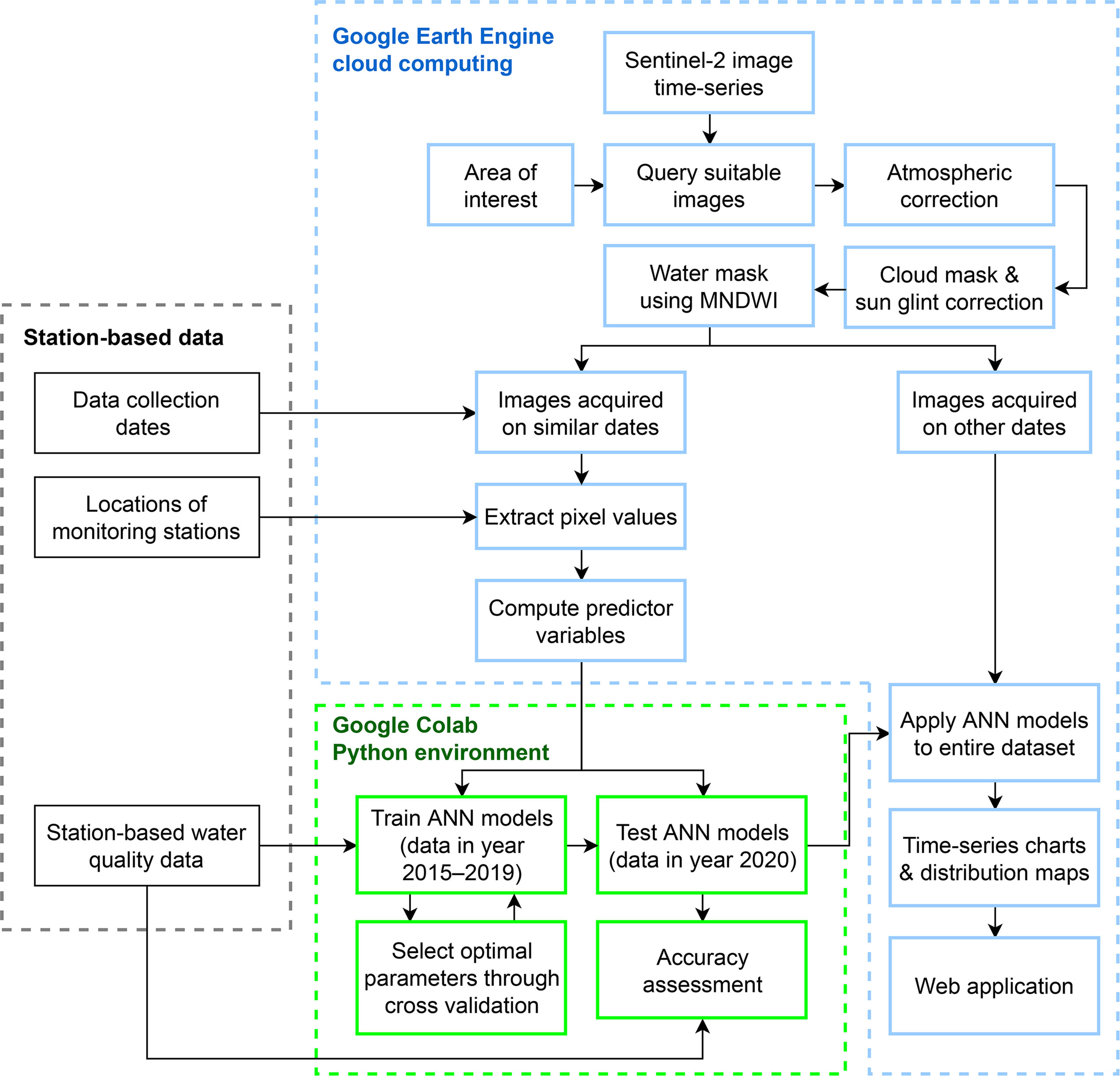
Figure 2 Flowchart of the proposed framework to estimate water quality parameters using Google Earth Engine (GEE) cloud computing platform and artificial neural network (ANN) algorithm. (MNDWI, Modified Normalized Difference Water Index).
Results and Discussion
Evaluation of ANN Regression Models for All Water Quality Parameters
Table 4 shows the evaluation metrics for the ANN models, including both model calibration and validation sets, developed for each of the 22 water quality parameters. The ANN models, optimized through cross-validations, selected a wide range of numbers of input variables and neurons for different parameters. For instance, the models developed for salinity and turbidity used 8 input variables and 2 neurons in a single hidden layer, indicating that the dependent variables correlated well with the predictors and can be estimated using relatively simple networks. Contrastingly, the modeling of parameters such as silica and Chl-a utilized 9–11 variables with 6–8 neurons in two hidden layers. Despite the complex network, the modeling results were promising for these parameters. When the training dataset was considered, correlation coefficients greater than 0.8 were obtained for salinity, SS, nitrate nitrogen, total inorganic nitrogen, silica and Chl-a. Among these six parameters, five of them (except SS) could produce r ≥ 0.845 in the validation set as well. This proved the applicability of ANN to develop regression models and predict the values of particular water quality parameters in this setting.
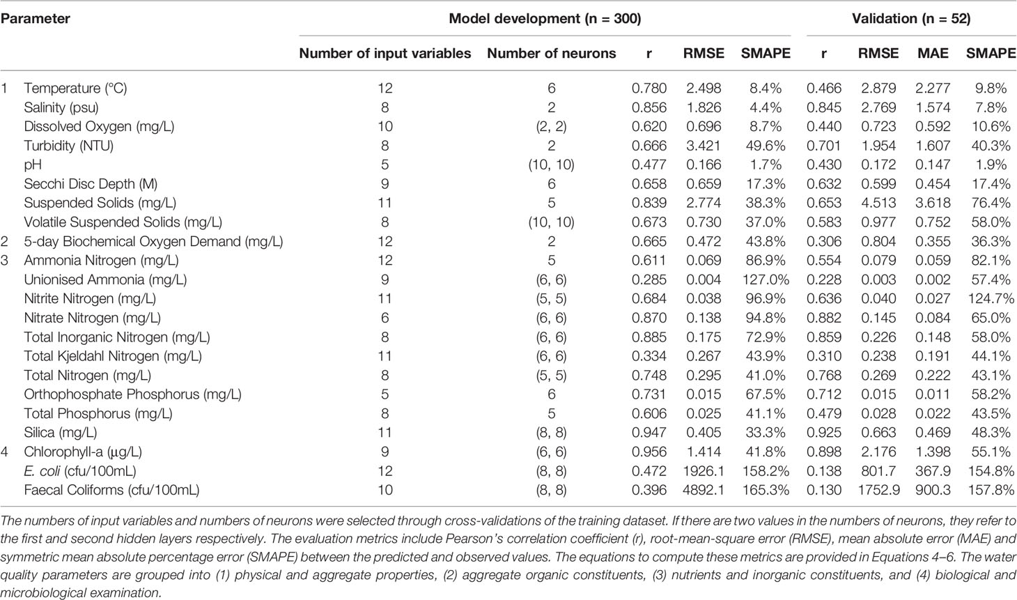
Table 4 Modeling results of the 22 water quality parameters calculated using artificial neural networks (ANN) on both training and validation datasets.
The water quality parameters investigated in this study could be categorized into physical properties, nutrient and inorganic constituents, and biological and microbiological examination. Results of the ANN models revealed that there was no clear pattern on the superiority of predicting particular groups of parameters. The physical properties of waters generally had moderate relationships with the spectral reflectance and the r values lied between 0.430 (pH) and 0.845 (salinity). The group of nutrient and inorganic constituents resulted in a wider range of r values from 0.228 (unionized ammonia) to 0.925 (silica). For biological and microbiological constituents, while Chl-a concentration led to a prediction model with promising fit (r = 0.898), E. coli and Faecal Coliforms generated the poorest results among all parameters tested in this study, with very weak correlations (r = 0.130–0.138) and large deviations (SMAPE = 154.8–157.8%) from the actual values. Although some scholars had reported substantial performance when applying regression models to estimate non-optical parameters including dissolved oxygen (Pizani et al., 2020), the agreement was not found in this study (r = 0.440). This could be explained by the complexity of coastal waters and the lack of consideration of interrelated optical properties among parameters (Kim et al., 2020).
From remote sensing perspective, some water quality parameters were considered as optically active components (Sobel et al., 2020), such as Chl-a and SS, which cause changes to the spectral properties of reflected light and are thus remotely detectable. Reviews by Gholizadeh et al. (2016) and Wang and Yang (2019) suggested that most of the existing studies concentrated on these optically active variables while other parameters without explicit optical properties were not well investigated. This study attempted to apply the same regression approach to all parameters and revealed a significant difference in the model performances in terms of correlation and other evaluation metrics. The findings in this study did not support that water quality parameters related to physical properties of water would produce better prediction performances compared to those related to nutrient and inorganic constituents. Instead, the potential to predict the levels of several types of nutrients and chemicals such as total nitrogen (r = 0.768), orthophosphate phosphorus (r = 0.712) and silica (r = 0.925) was also suggested. Nevertheless, since these water quality parameters were seldom studied using remote sensing methods (Gholizadeh et al., 2016), their spectral responses and modeling potentials would need to be further investigated.
Based on the ANN modeling results, the following sections would focus on three water quality parameters, namely Chl-a, SS and turbidity, which had relatively accurate estimations and strong relationships with the predictor variables. This also allowed in-depth analysis of the remote sensing-based techniques since these parameters have been investigated in similar studies.
Variables Used in Chl-a, SS and Turbidity Models
The variables used as inputs in the ANN models for Chl-a, SS and turbidity are described in Table 5. Through cross-validations, each model selected 8–11 predictors which provided relatively high correlations with the dependent variables. For the Chl-a model, it adopted a combination of band 1 (coastal aerosol), band 2 (blue), band 8A (NIR), blue-green ratio, three-band ratio of band 2, band 3 (green) and band 4 (red), as well as line-heights of band 2, band 4 and band 8A.
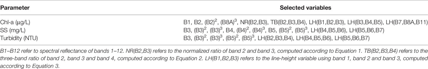
Table 5 The variables selected as inputs in the ANN models developed in this study for chlorophyll-a (Chl-a), suspended solids (SS) and turbidity.
As suggested in existing literature, there is little consistency in the effectiveness of different bands or band ratios in estimating various water quality parameters, which further depends on the parameter ranges and study areas (Matthews, 2011; Topp et al., 2020). For instance, although band 5 in Sentinel-2 corresponds to a well-known reflectance peak of Chl-a near 705 nm in high-biomass waters (Gons, 1999), none of the band combinations directly associated with this wavelength was selected in the model. While the three-band ratio variables were originally constructed using the red-edge wavelengths from 665 to 740 nm and were shown to be useful in Ansper and Alikas (2019) and Free et al. (2020), it became one of the significant predictors of Chl-a when the same equation was applied to the visible bands in the present study. These were coherent with previous studies of Hong Kong water, which proved that a locally calibrated model outperformed models established in other study areas including the standard Case-2 Regional/Coast Color (C2RCC) processing chain model (Hafeez et al., 2019).
Despite the variety of predictor combinations, the selected variables were consistent with the prominent spectral characteristics such as absorption and scattering features of the optical constituents. As shown in the Chl-a model, 6 out of the 9 selected variables were related to coastal aerosol, blue and green bands and blue-green ratio, which represented the theoretical behavior of Chl-a that absorbs blue lights and reflects green lights (Soriano-González et al., 2019). The properties were more evident for dinoflagellates and diatoms (Sadeghi et al., 2012), the two major phytoplankton classes present in Hong Kong waters (Cheung et al., 2021). The incorporation of band 8A also matched the observation by other studies that NIR bands could be helpful to separate Chl-a from other constituents in turbid coastal waters (Hafeez et al., 2019; Ouma et al., 2020).
For the SS and turbidity models, the selected variables were dominated by those generated from green, red and red-edge bands, their square and cubic values, as well as their line-heights against neighboring bands. Similarly, refractive index and grain size of SS in Hong Kong waters were found to be sensitive to the green and red wavelengths in previous work (Nazeer and Nichol, 2015). Red-edge wavelength also becomes influential when inorganic SS concentrations increase in turbid waters (Topp et al., 2020). For turbidity, algorithms involving the red band are generally adopted owing to the scattering of particulates (Matthews, 2011). In this study, it was interesting that 7 out of 8–11 variables appeared in both SS and turbidity models, and they used small numbers of neurons (2–5) in the single hidden layer. This provided another piece of evidence that these two water quality parameters are closely related to each other and have relatively simple relationships with spectral variables.
Performances of Chl-a, SS and Turbidity Models
Figure 3 compares the predicted and observed Chl-a, SS and turbidity values using both the training and validation datasets. While the ANN models performed well in the training phase as shown in the correspondence between the fitted lines and the one-to-one lines, overfitting was also not a problem in the models since they generated similar performances when applied to the independent validation sets. Considering the validation performance, for Chl-a, the ANN model was able to accurately predict a data point with high observed value, which likely represents an occasional algal bloom event. Further analysis using Spearman’s correlation showed that the correspondence between the predicted and observed values was also satisfactory without the effect of this outlier point. However, the model tended to slightly underestimate the Chl-a concentrations when the observed values were below 4 μg/L. For SS, while the fitted line corresponds well with the one-to-one line, Pearson’s correlation coefficient was lower (r = 0.653), probably due to the larger spread of values around the fitted line (RMSE = 4.513 mg/L, SMAPE = 76.4%). In contrast to Chl-a, the model tended to overestimate the SS values when the actual values were low (< 4 mg/L) and this pattern was visible in both the training and validation datasets. For turbidity, the agreement was also strong in terms of correlation coefficient (r = 0.701) and other error metrics (RMSE = 1.954 NTU, SMAPE = 40.3%). Nonetheless, when the observed values were large, overestimation could be an issue found from the scatterplot.
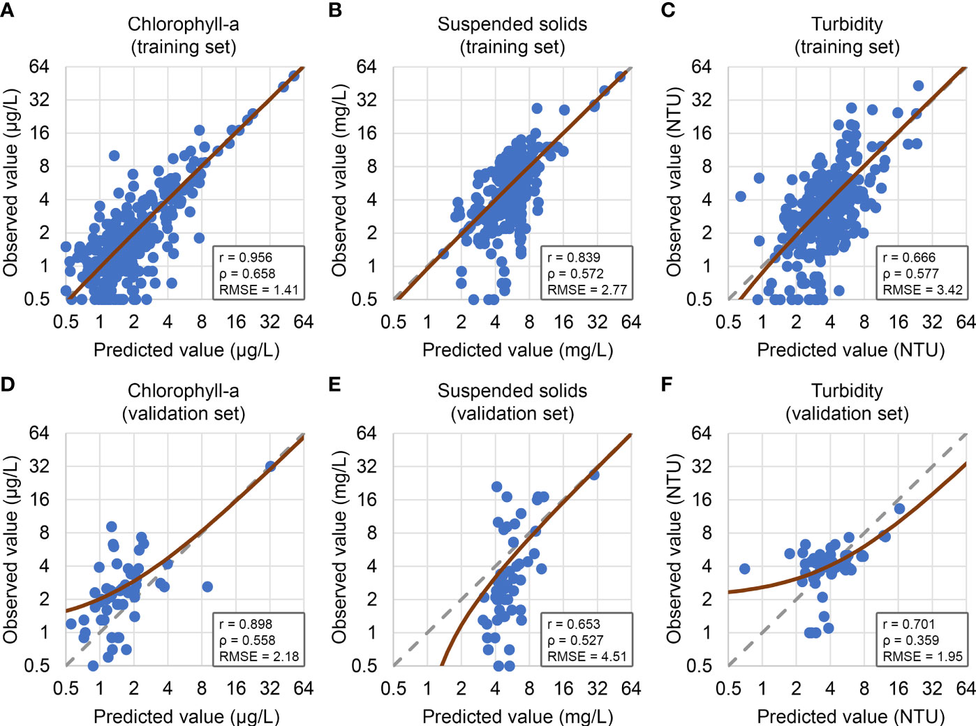
Figure 3 Scatterplots comparing the predicted and observed values of chlorophyll-a, suspended solids and turbidity using the training set (A–C) and validation set (D–F). The gray dotted lines indicate the one-to-one relationships and the red lines indicate the best-fitting lines. Note that the x- and y-axes are in logarithmic scale, while the best-fitting lines and all statistics are calculated based on the untransformed scale. Besides Pearson’s correlation coefficient (r) and root-mean-square error (RMSE), Spearman’s rank correlation (ρ) is also computed to provide a measure with lower sensitivity to outliers in the dataset.
The prediction errors for Chl-a found in this study (55.1%) exceeded the desired relative error of 35% set by NASA’s Ocean Biology and Biogeochemistry Program (McCain et al., 2006). However, the standard was specified for open ocean dominated by phytoplankton. Coastal and estuarine waters are commonly referred to as Case-2 waters (Morel and Prieur, 1977), with optical properties significantly influenced by various constituents including yellow substance and suspended materials, thus were expected to be challenging to develop algorithms for predicting water quality parameters.
To serve as a benchmark of the performance, modeling results were extracted from previous works on Hong Kong water and the accuracies were found to vary for different parameters (Table 6). For Chl-a, the results were comparable and had similar levels of correlations and errors. While the prediction of SS seemed to be less satisfactory than those obtained from previous methods, the prediction of turbidity produced lower correlation but lower errors as well. This comparison indicated that, in addition to the modeling algorithm, the selection of input data and pre-processing steps were more influential on the results.
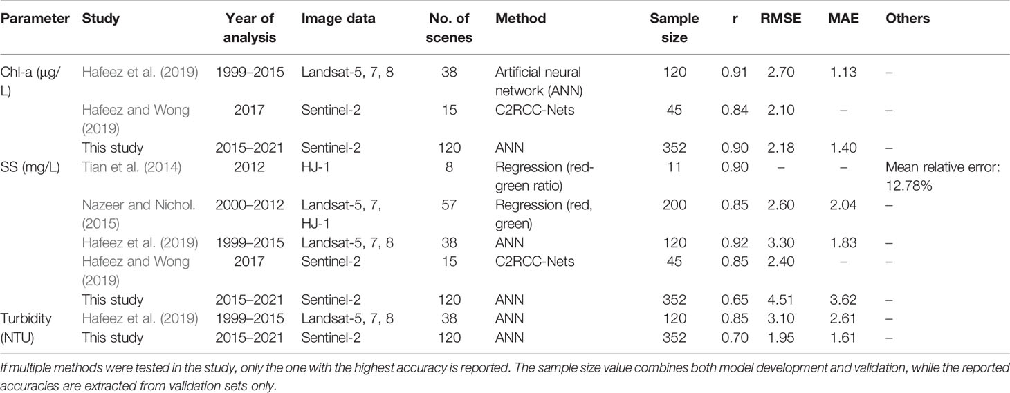
Table 6 Comparison of modeling results with other studies focusing on Hong Kong waters.
In view of this, the findings presented in this study were encouraging considering the following aspects: (i) This study represented an operational context that extracted all available images acquired by Sentinel-2A/B satellites, matched with station-based measurement and applied a fully automatic analysis workflow with the capability of GEE; (ii) While linear regression analysis is more popular in GEE due to easy implementation (Tamiminia et al., 2020), the use of ANN algorithm through this platform enabled manipulation of non-linear relationships (Forkuor et al., 2017) and rapid estimation of water quality parameters when new images become available; (iii) This study was more robust than previous works in the same study area, due to the larger number of observations and extensive use of images from different years and months, facilitating the applicability over the spatially and temporally variable water conditions; (iv) Besides the commonly used RMSE and MAE, this study also reported relative errors which enable meaningful comparisons across models developed in different water regions (Shcherbakov et al., 2013).
Visualization of Model Performance Using Time-Series Charts
The developed models were applied to all Sentinel-2 images to produce spatial distribution maps of Chl-a, SS and turbidity from 2015 to 2021. To visualize the temporal patterns of these water quality parameters, time-series charts were generated by plotting the average values estimated from each remotely-sensed image against time (Figure 4). The line graph illustrated that the shapes and magnitudes of remote sensing estimates generally matched well with station-based measurements. For example, the temporal changes of Chl-a concentration showed higher values commonly found during summer, which were revealed from both remote sensing estimation and station-based measurement. From the line graph, some of the peaks found from station-based measurements could also be obtained using remote sensing estimation, showing that the method proposed in this study could capture some of the extreme events as well. It should also be noted that differences in sampling locations and frequencies of the two measurement methods could affect their correspondence presented in the graph.
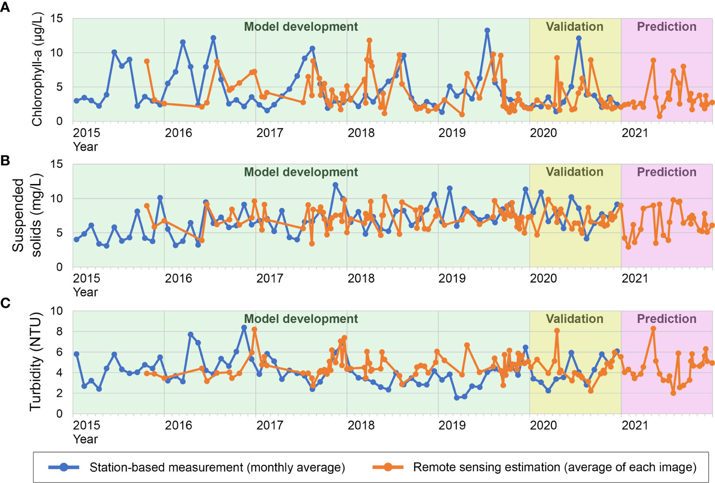
Figure 4 Time-series line chart of (A) chlorophyll-a concentration, (B) suspended solids, and (C) turbidity in Hong Kong water from 2015 to 2021, obtained from station-based measurement (blue lines) and remote sensing estimation (orange lines) respectively. For station-based measurement, values are calculated as the mean value of all measurements in all locations taken in the same month. For remote sensing estimations, values are calculated as the mean of all estimated values at the locations of monitoring stations in each image. Note that the two measurement methods also differ in sampling locations (e.g. affected by cloud cover and water pixels) and frequencies (e.g. image acquisition dates).
As shown in Figure 4, the temporal range in this study was separated into model development (2015–2019), validation (2020) and prediction (2021) according to the developed methodology. Historical observations are valuable in time-series to estimate the model coefficients, followed by predicting new values and identifying abnormal changes in the monitoring period (Hamunyela et al., 2020; Elhag et al., 2021). This was also demonstrated in this study and water qualities in later years were estimated using models calibrated from previous data. Since the data release of station-based measurement by the Hong Kong government usually has a time lag of more than half a year, continuous monitoring of the latest year (2021 in this study) could be complemented by the remote sensing approach.
Spatial and Temporal Variations of Chl-a, SS and Turbidity Across Hong Kong Waters
The spatial and seasonal variabilities in the whole study area are also visualized through high-resolution maps (Figure 5). In all seasons, it showed higher SS loads and turbidity in the western part compared to the eastern waters, mainly due to the contrasting effects of Pearl River discharge from the west and oceanic currents from the east (Lai et al., 2016). High values particularly during spring and summer, as a consequence of the southwest monsoon and strong riverine inputs (Environmental Protection Department, 2021), were also evidenced in the maps. The high Chl-a concentrations in the shallow waters of Deep Bay were consistent with those revealed in Hafeez et al. (2019) (8.0–15.6 μg/L), owing to domestic wastewater and agricultural runoff (Zhou et al., 2007).
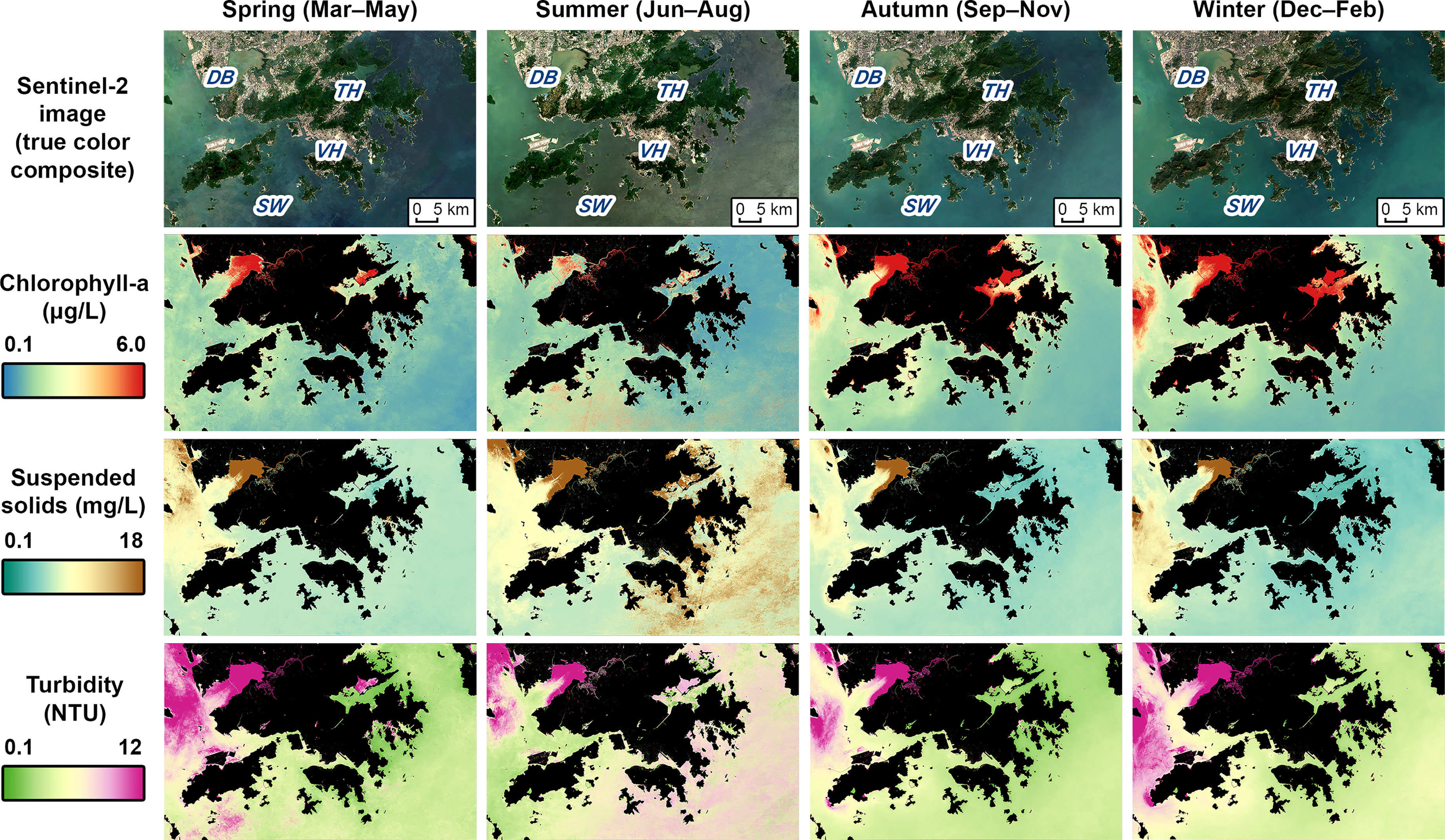
Figure 5 Spatial distribution maps of chlorophyll-a concentration, suspended solids and turbidity in Hong Kong water in the four seasons, calculated as the mean value of all remote sensing-based estimations within each meteorological season in 2015–2021. (DB, Deep Bay; VH, Victoria Harbour; TH, Tolo Harbour; SW, Southern Water).
In Victoria Harbour, while moderate values of Chl-a (7.0–10.0 μg/L) were reported in Hafeez et al. (2019), this study tended to observe lower concentrations on average (2.0–4.0 μg/L). This was probably because the present study utilized a larger number of images and Chl-a concentration tends to remain at low levels with high flushing rates most of the time throughout the year (Xu et al., 2010). Tolo Harbour, a land-locked inlet located in northeastern Hong Kong, was suggested to have highly eutrophic water and regular algal blooms due to restricted water exchange, low tidal flushing and persistent stratification (Lai et al., 2016). The maps produced in this study provided further observations that high Chl-a concentrations in that area tended to occur more frequently in autumn and winter. This seasonal variation matched with the findings of a recent forecasting study by Deng et al. (2022) and could be related to the downwelling process and concentration of algal biomass in that period (Xu et al., 2010). In the southern waters, slightly higher Chl-a concentrations were observed in summer from the produced maps, which also agrees with the observations by Zhou et al. (2012) that these areas represent the estuarine coastal frontal region and favor the development of algal blooms in July and August.
Besides seasonal trends, the robustness of the developed model was further demonstrated when applied on a particular occasion. During a red tide incident that occurred in Victoria Harbour from 13th to 16th July 2020 caused by phytoplankton species Amphora spp. (Agriculture, Fisheries and Conservation Department, 2021), the Chl-a concentration map produced from the Sentinel-2 image acquired on 13th Jul 2020 successfully revealed high values in that location (Figure 6). The estimated Chl-a values in the nearby areas were also consistent with station-based measurements within the same period. While moderate to high concentrations were found in Victoria Harbour and North Western Water Control Zones, the map was able to present low concentrations, on the contrary, in Port Shelter at the same period. These results again confirmed the prediction ability in the monitoring period using models calibrated from historical data, where potential anomalies in water conditions including algal bloom events and their spatial variabilities could be captured.
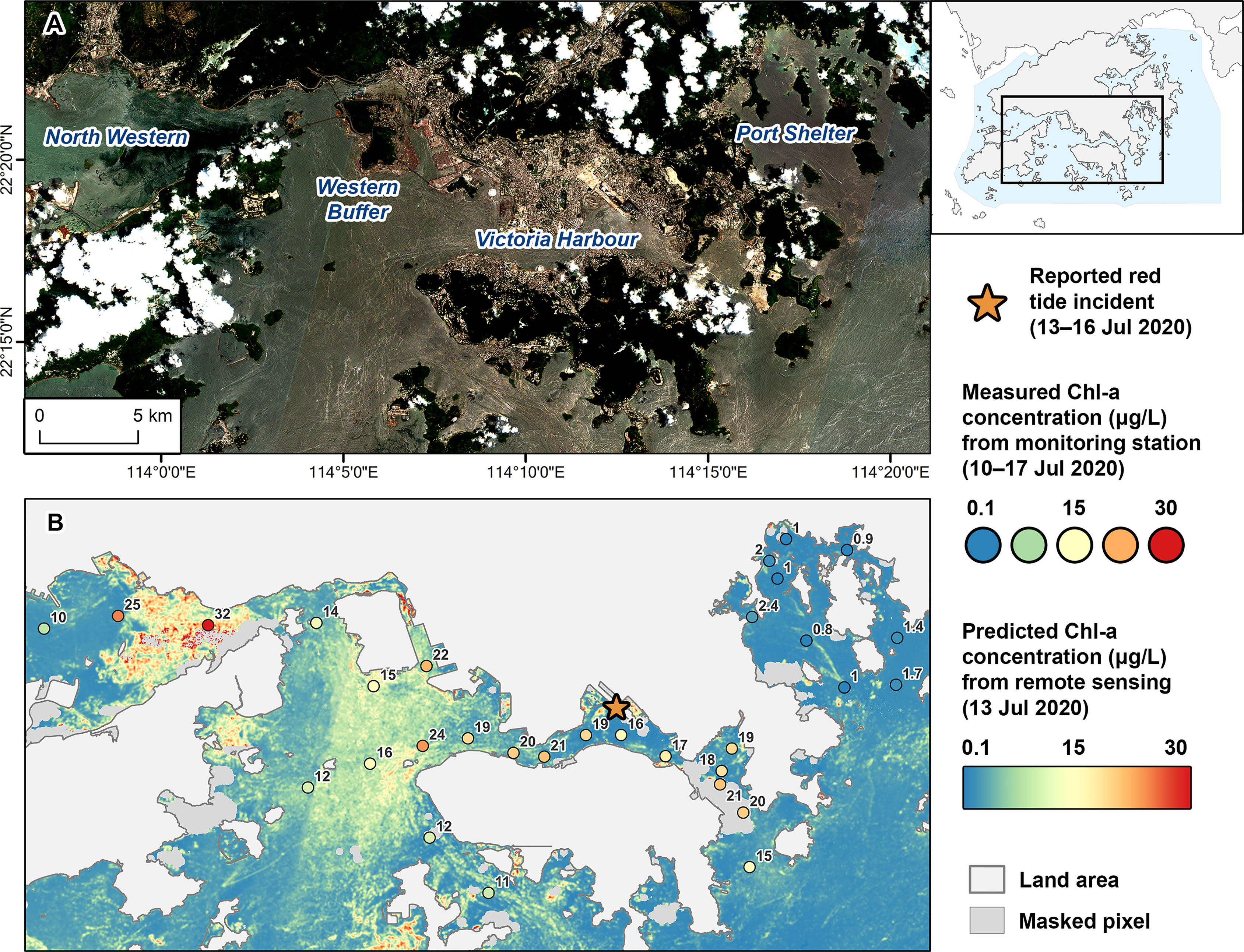
Figure 6 (A) True color composite of Sentinel-2 image acquired on 13th July 2020 and (B) the estimated chlorophyll-a (Chl-a) concentration map, overlaid with in situ data measured in the monitoring stations.
Customized GEE Application
Finally, using functions available in GEE, an online application was created (https://khoyinivan.users.earthengine.app/view/marine-water-quality-hk) to allow users to explore and analyze water quality trends with a simple web interface (Figure 7). Besides zooming and panning the map to show different locations, users can interact with the applications in several ways, including displaying the concentration map of water quality parameters for a specific date and plotting time-series charts of parameters for a specific location.
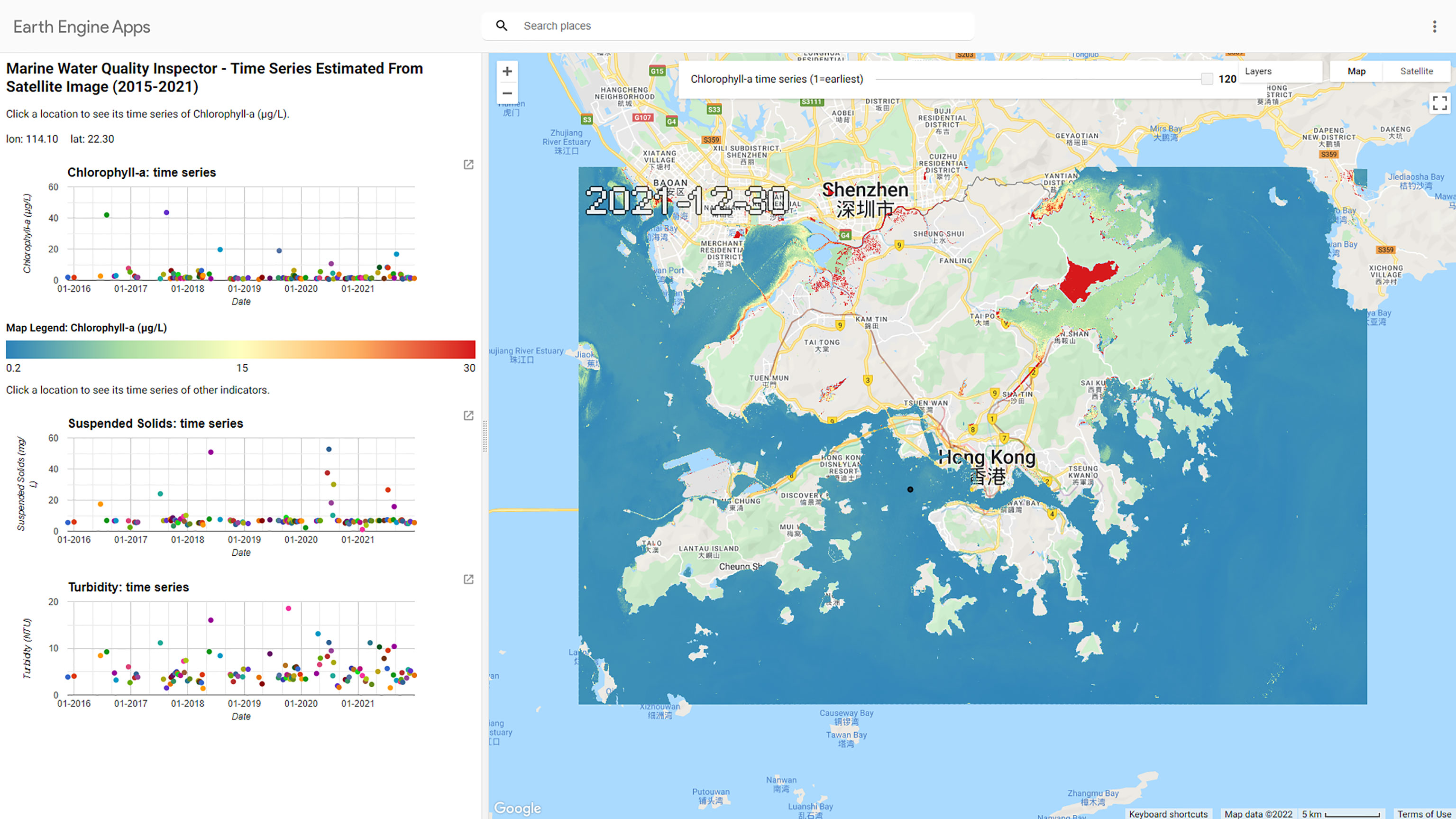
Figure 7 A screenshot of the developed online application in Google Earth Engine showing the water quality map for a specific date and time-series charts for a specific location.
Achievements and Limitations of This Study
The online application, together with the analysis workflow, takes advantage of the cloud computing GEE infrastructure and the readily available Sentinel-2 satellite images. In this study, the comprehensive archive of Sentinel-2 dataset was seamlessly searched and processed in the cloud platform, without the need for downloading image data as in the conventional processing approach (Kumar and Mutanga, 2018; Li et al., 2021). The method is cost-effective as the Sentinel-2 data, GEE and Python software are open-source and freely available. Sentinel-2 will revisit the study area every five days with the two-satellite constellation and become available in GEE (Rudiyanto et al., 2019). Since the mapping processes can also be implemented automatically with the algorithm coded in GEE and Python, this enables monitoring from continuously updated remote sensing datasets in a timely manner and generates actionable information for decision-making (Markert et al., 2018; Page et al., 2019). Although the obtained levels of accuracies were below the desired standard, the end-to-end cloud computing workflow demonstrated in this study should be investigated considering the cost and computational efficiency for rapid information delivery.
The developed methodology and GEE scripts can further be extended to larger scales to increase usability and transferability (Kumar and Mutanga, 2018). It was anticipated that integrated use of remote sensing, in situ measurements and computer modeling can lead to an enhanced knowledge of the water quality (Gholizadeh et al., 2016). Still, the remote sensing tool would require support from existing in situ monitoring infrastructure and established laboratories (Pompêo et al., 2021). Hence, the routine measurements of biophysical and chemical properties of water by EPD of the Hong Kong government provide great opportunities for experimentation in this study.
Nevertheless, the remote sensing approach is limited by satellite repeat cycles and cloud coverage. Sent et al. (2021) described that in their work, only 55% of the total images available over the 2-year study period were cloud-free and in good atmospheric conditions. The percentage was even smaller (31.7%, 120 out of 379 images) in this study (Table 3), due to the subtropical oceanic monsoon climate in Hong Kong (Tian et al., 2014). Moreover, the image availability was non-homogeneous throughout the year with fewer images available in the wet season (spring and summer), making routine water monitoring even more challenging. Future work can explore the combined use with other satellite missions, such as Landsat satellites (Page et al., 2019), to enhance the observing capability.
Another limitation in the model development process in this study was the lack of in situ reflectance data. The calibration and evaluation of the algorithms were performed solely using satellite-based reflectance and station-based water quality measurements, which inhibited the understanding of the atmospheric influence and the true relationships between water-leaving reflectance and water quality parameters (Yoon et al., 2019). As illustrated in Kuhn et al. (2019), 70–90% of the signals in water pixels came from atmospheric effects and the choice of correction methods could bias parameter retrieval accuracies, posing challenges to land observation satellites like Sentinel-2. Adjacency to land areas further affected the optical complexity of coastal waters and hindered the use of algorithms developed for open oceans (Moses et al., 2017), as evidenced by the high NIR and SWIR reflectance of water pixels in this study. Many scholars have performed intercomparison of various atmospheric correction and bio-optical algorithms (Gernez et al., 2017; Poddar et al., 2019; Soomets et al., 2020; Sent et al., 2021), using both in situ and satellite measurements, to assess the retrieval performances in specific regional waters. Future work can focus on the identification of optimal algorithms for predicting water quality parameters, including both optically active and inactive parameters, that can be incorporated into GEE applications for operational monitoring.
Conclusion
Using coastal waters of Hong Kong as the study area, this study utilized GEE to (i) query and pre-process all Sentinel-2 observations that coincided with in situ measurements; (ii) extract the spectra to develop empirical models for different water quality parameters using ANN; and (iii) present the results using spatial distribution maps, time-series charts and an online application. Together these features enabled novice users to discover, analyze and visualize spatial and temporal patterns from remotely-sensed images. This study demonstrated that the integration of Sentinel-2 satellite images, in situ measurements and the GEE cloud computing platform can offer new opportunities for providing cost-effective and timely prediction of water quality parameters. With multiple water quality parameters analyzed in this study, the mapping results could help comprehensive understanding the dynamics of water qualities within the study area in multiple years, raise awareness of environmental changes in relation to human activities and promote sound management policies. When longer records of both water quality measurements and freely available earth observation data become available in the future, more integrated and robust predictive models can be developed to continue to contribute towards an effective water resource monitoring framework.
Data Availability Statement
Publicly available datasets were analyzed in this study. This data can be found here: https://github.com/ivanhykwong/marine-water-quality-time-series-hk.
Author Contributions
IK and FW initiated this study. IK designed the methods, conducted the analysis, and drafted the manuscript. FW and TF supervised the work and improved on the result interpretation. All authors contributed to the article and approved the submitted version.
Conflict of Interest
The authors declare that the research was conducted in the absence of any commercial or financial relationships that could be construed as a potential conflict of interest.
Publisher’s Note
All claims expressed in this article are solely those of the authors and do not necessarily represent those of their affiliated organizations, or those of the publisher, the editors and the reviewers. Any product that may be evaluated in this article, or claim that may be made by its manufacturer, is not guaranteed or endorsed by the publisher.
Acknowledgments
The authors would like to thank the Environmental Protection Department (EPD) of the Hong Kong government for providing station-based coastal water quality data. Sentinel-2 image archive was provided by the European Space Agency (ESA) and acquired through the Google Earth Engine API. We thank the editors and all reviewers for their valuable comments on this manuscript.
References
Agriculture, Fisheries and Conservation Department (2021) Hong Kong Red Tide Database. Available at: https://redtide.afcd.gov.hk/urtin/#/maps?mode=1&lang=en (Accessed 31 January 2022).
Amani M., Kakooei M., Moghimi A., Ghorbanian A., Ranjgar B., Mahdavi S., et al. (2020). Application of Google Earth Engine Cloud Computing Platform, Sentinel Imagery, and Neural Networks for Crop Mapping in Canada. Remote Sens. 12 (21), 3561. doi: 10.3390/rs12213561
Ansper A., Alikas K. (2019). Retrieval of Chlorophyll a From Sentinel-2 MSI Data for the European Union Water Framework Directive Reporting Purposes. Remote Sens. 11 (1), 64. doi: 10.3390/rs11010064
Atkinson P. M., Tatnall A. R. L. (1997). Introduction Neural Networks in Remote Sensing. Int. J. Remote Sens. 18 (4), 699–709. doi: 10.1080/014311697218700
Canty M. J., Nielsen A. A., Conradsen K., Skriver H. (2020). Statistical Analysis of Changes in Sentinel-1 Time Series on the Google Earth Engine. Remote Sens. 12 (1), 46. doi: 10.3390/rs12010046
Chebud Y., Naja G. M., Rivero R. G., Melesse A. M. (2012). Water Quality Monitoring Using Remote Sensing and an Artificial Neural Network. Water Air. Soil Pollut. 223 (8), 4875–4887. doi: 10.1007/s11270-012-1243-0
Chen X., Li Y. S., Liu Z., Yin K., Li Z., Wai O. W. H., et al. (2004). Integration of Multi-Source Data for Water Quality Classification in the Pearl River Estuary and its Adjacent Coastal Waters of Hong Kong. Cont. Shelf. Res. 24 (16), 1827–1843. doi: 10.1016/j.csr.2004.06.010
Chen C., Twycross J., Garibaldi J. M. (2017). A New Accuracy Measure Based on Bounded Relative Error for Time Series Forecasting. PloS One 12 (3), e0174202. doi: 10.1371/journal.pone.0174202
Cheung Y. Y., Cheung S., Mak J., Liu K., Xia X., Zhang X., et al. (2021). Distinct Interaction Effects of Warming and Anthropogenic Input on Diatoms and Dinoflagellates in an Urbanized Estuarine Ecosystem. Glob. Change Biol. 27 (15), 3463–3473. doi: 10.1111/gcb.15667
Dall’Olmo G., Gitelson A. A. (2005). Effect of Bio-Optical Parameter Variability on the Remote Estimation of Chlorophyll-a Concentration in Turbid Productive Waters: Experimental Results. Appl. Opt. 44 (3), 412–422. doi: 10.1364/AO.44.000412
Deng T., Duan H.-F., Keramat A. (2022). Spatiotemporal Characterization and Forecasting of Coastal Water Quality in the Semi-Enclosed Tolo Harbour Based on Machine Learning and EKC Analysis. Eng. Appl. Comput. Fluid. Mech. 16 (1), 694–712. doi: 10.1080/19942060.2022.2035257
Drusch M., Del Bello U., Carlier S., Colin O., Fernandez V., Gascon F., et al. (2012). Sentinel-2: ESA's Optical High-Resolution Mission for GMES Operational Services. Remote Sens. Environ. 120, 25–36. doi: 10.1016/j.rse.2011.11.026
Elhag M., Gitas I., Othman A., Bahrawi J., Psilovikos A., Al-Amri N. (2021). Time Series Analysis of Remotely Sensed Water Quality Parameters in Arid Environments, Saudi Arabia. Environ. Dev. Sustain. 23 (2), 1392–1410. doi: 10.1007/s10668-020-00626-z
Environmental Protection Department (2021) Marine Water Quality in Hong Kong in 2020. Available at: https://www.epd.gov.hk/epd/sites/default/files/epd/english/environmentinhk/water/hkwqrc/files/waterquality/annual-report/marinereport2020.pdf (Accessed 31 January 2022).
Flores-Anderson A. I., Griffin R., Dix M., Romero-Oliva C. S., Ochaeta G., Skinner-Alvarado J., et al. (2020). Hyperspectral Satellite Remote Sensing of Water Quality in Lake Atitlán, Guatemala. Front. Environ. Sci. 8 (7). doi: 10.3389/fenvs.2020.00007
Forkuor G., Hounkpatin O. K. L., Welp G., Thiel M. (2017). High Resolution Mapping of Soil Properties Using Remote Sensing Variables in South-Western Burkina Faso: A Comparison of Machine Learning and Multiple Linear Regression Models. PloS One 12 (1), e0170478. doi: 10.1371/journal.pone.0170478
Free G., Bresciani M., Trodd W., Tierney D., O’Boyle S., Plant C., et al. (2020). Estimation of Lake Ecological Quality From Sentinel-2 Remote Sensing Imagery. Hydrobiologia 847 (6), 1423–1438. doi: 10.1007/s10750-020-04197-y
Gernez P., Doxaran D., Barillé L. (2017). Shellfish Aquaculture From Space: Potential of Sentinel2 to Monitor Tide-Driven Changes in Turbidity, Chlorophyll Concentration and Oyster Physiological Response at the Scale of an Oyster Farm. Front. Mar. Sci. 4 (137). doi: 10.3389/fmars.2017.00137
Gholizadeh M. H., Melesse A. M., Reddi L. (2016). A Comprehensive Review on Water Quality Parameters Estimation Using Remote Sensing Techniques. Sensors 16 (8), 1298. doi: 10.3390/s16081298
Ghorbanian A., Ahmadi S. A., Amani M., Mohammadzadeh A., Jamali S. (2022). Application of Artificial Neural Networks for Mangrove Mapping Using Multi-Temporal and Multi-Source Remote Sensing Imagery. Water 14 (2), 244. doi: 10.3390/w14020244
Gitelson A., Mayo M., Yacobi Y. Z., Parparov A., Berman T. (1994). The Use of High-Spectral-Resolution Radiometer Data for Detection of Low Chlorophyll Concentrations in Lake Kinneret. J. Plankton. Res. 16 (8), 993–1002. doi: 10.1093/plankt/16.8.993
Gons H. J. (1999). Optical Teledetection of Chlorophyll a in Turbid Inland Waters. Environ. Sci. Technol. 33 (7), 1127–1132. doi: 10.1021/es9809657
Gorelick N., Hancher M., Dixon M., Ilyushchenko S., Thau D., Moore R. (2017). Google Earth Engine: Planetary-Scale Geospatial Analysis for Everyone. Remote Sens. Environ. 202, 18–27. doi: 10.1016/j.rse.2017.06.031
Gower J. F. R., Doerffer R., Borstad G. A. (1999). Interpretation of the 685nm Peak in Water-Leaving Radiance Spectra in Terms of Fluorescence, Absorption and Scattering, and Its Observation by MERIS. Int. J. Remote Sens. 20 (9), 1771–1786. doi: 10.1080/014311699212470
Gower J., King S., Borstad G., Brown L. (2005). Detection of Intense Plankton Blooms Using the 709 Nm Band of the MERIS Imaging Spectrometer. Int. J. Remote Sens. 26 (9), 2005–2012. doi: 10.1080/01431160500075857
Hafeez S., Wong M. S. (2019). "Measurement of Coastal Water Quality Indicators Using Sentinel-2; An Evaluation Over Hong Kong and the Pearl River Estuary", in: IGARSS 2019 - 2019 IEEE International Geoscience and Remote Sensing Symposium), 8249-8252. doi: 10.1109/IGARSS.2019.8899342
Hafeez S., Wong M. S., Ho H. C., Nazeer M., Nichol J., Abbas S., et al. (2019). Comparison of Machine Learning Algorithms for Retrieval of Water Quality Indicators in Case-II Waters: A Case Study of Hong Kong. Remote Sens. 11 (6), 617. doi: 10.3390/rs11060617
Hamunyela E., Rosca S., Mirt A., Engle E., Herold M., Gieseke F., et al. (2020). Implementation of BFASTmonitor Algorithm on Google Earth Engine to Support Large-Area and Sub-Annual Change Monitoring Using Earth Observation Data. Remote Sens. 12 (18), 2953. doi: 10.3390/rs12182953
Hu C., Feng L., Lee Z., Davis C. O., Mannino A., McClain C. R., et al. (2012). Dynamic Range and Sensitivity Requirements of Satellite Ocean Color Sensors: Learning From the Past. Appl. Opt. 51 (25), 6045–6062. doi: 10.1364/AO.51.006045
Jia M., Wang Z., Mao D., Ren C., Wang C., Wang Y. (2021). Rapid, Robust, and Automated Mapping of Tidal Flats in China Using Time Series Sentinel-2 Images and Google Earth Engine. Remote Sens. Environ. 255, 112285. doi: 10.1016/j.rse.2021.112285
Kay S., Hedley J. D., Lavender S. (2009). Sun Glint Correction of High and Low Spatial Resolution Images of Aquatic Scenes: A Review of Methods for Visible and Near-Infrared Wavelengths. Remote Sens. 1 (4), 697–730. doi: 10.3390/rs1040697
Khan R. M., Salehi B., Mahdianpari M., Mohammadimanesh F. (2021). Water Quality Monitoring Over Finger Lakes Region Using Sentinel-2 Imagery on Google Earth Engine Cloud Computing Platform. ISPRS Ann. Photogramm. Remote Sens. Spatial. Inf. Sci. V-3-2021, 279–283. doi: 10.5194/isprs-annals-V-3-2021-279-2021
Kim Y. H., Son S., Kim H.-C., Kim B., Park Y.-G., Nam J., et al. (2020). Application of Satellite Remote Sensing in Monitoring Dissolved Oxygen Variabilities: A Case Study for Coastal Waters in Korea. Environ. Int. 134, 105301. doi: 10.1016/j.envint.2019.105301
Kuhn C., de Matos Valerio A., Ward N., Loken L., Sawakuchi H. O., Kampel M., et al. (2019). Performance of Landsat-8 and Sentinel-2 Surface Reflectance Products for River Remote Sensing Retrievals of Chlorophyll-a and Turbidity. Remote Sens. Environ. 224, 104–118. doi: 10.1016/j.rse.2019.01.023
Kumar L., Mutanga O. (2018). Google Earth Engine Applications Since Inception: Usage, Trends, and Potential. Remote Sens. 10 (10), 1509. doi: 10.3390/rs10101509
Lai R. W. S., Perkins M. J., Ho K. K. Y., Astudillo J. C., Yung M. M. N., Russell B. D., et al. (2016). Hong Kong’s Marine Environments: History, Challenges and Opportunities. Reg. Stud. Mar. Sci. 8, 259–273. doi: 10.1016/j.rsma.2016.09.001
Li J., Peng B., Wei Y., Ye H. (2021). Accurate Extraction of Surface Water in Complex Environment Based on Google Earth Engine and Sentinel-2. PloS One 16 (6), e0253209. doi: 10.1371/journal.pone.0253209
Liu H., Li Q., Shi T., Hu S., Wu G., Zhou Q. (2017). Application of Sentinel 2 MSI Images to Retrieve Suspended Particulate Matter Concentrations in Poyang Lake. Remote Sens. 9 (7), 761. doi: 10.3390/rs9070761
Markert K. N., Schmidt C. M., Griffin R. E., Flores A. I., Poortinga A., Saah D. S., et al. (2018). Historical and Operational Monitoring of Surface Sediments in the Lower Mekong Basin Using Landsat and Google Earth Engine Cloud Computing. Remote Sens. 10 (6), 909. doi: 10.3390/rs10060909
Matthews M. W. (2011). A Current Review of Empirical Procedures of Remote Sensing in Inland and Near-Coastal Transitional Waters. Int. J. Remote Sens. 32 (21), 6855–6899. doi: 10.1080/01431161.2010.512947
McCain C., Hooker S., Feldman G., Bontempi P. (2006). Satellite Data for Ocean Biology, Biogeochemistry, and Climate Research. Eos. Trans. AGU. 87 (34), 337–343. doi: 10.1029/2006EO340002
Morel A., Prieur L. (1977). Analysis of Variations in Ocean Color. Limnol. Oceanogr. 22 (4), 709–722. doi: 10.4319/lo.1977.22.4.0709
Moses W. J., Sterckx S., Montes M. J., De Keukelaere L., Knaeps E. (2017). “Chapter 3 - Atmospheric Correction for Inland Waters”, in Bio-Optical Modeling and Remote Sensing of Inland Waters. Eds. D.R M., I O., A.A G. (Amsterdam, Netherlands: Elsevier), 69–100.
Mouw C. B., Greb S., Aurin D., DiGiacomo P. M., Lee Z., Twardowski M., et al. (2015). Aquatic Color Radiometry Remote Sensing of Coastal and Inland Waters: Challenges and Recommendations for Future Satellite Missions. Remote Sens. Environ. 160, 15–30. doi: 10.1016/j.rse.2015.02.001
Murphy S. (2020) Atmospheric Correction of Sentinel 2 Imagery in Google Earth Engine Using Py6S. Available at: https://github.com/samsammurphy/gee-atmcorr-S2 (Accessed 31 January 2022).
Nazeer M., Nichol J. E. (2015). Combining Landsat TM/ETM+ and HJ-1 a/B CCD Sensors for Monitoring Coastal Water Quality in Hong Kong. IEEE Geosci. Remote. Sens. Lett. 12 (9), 1898–1902. doi: 10.1109/LGRS.2015.2436899
Nazeer M., Nichol J. E., Yung Y.-K. (2014). Evaluation of Atmospheric Correction Models and Landsat Surface Reflectance Product in an Urban Coastal Environment. Int. J. Remote Sens. 35 (16), 6271–6291. doi: 10.1080/01431161.2014.951742
Ouma Y. O., Noor K., Herbert K. (2020). Modelling Reservoir Chlorophyll-a, TSS, and Turbidity Using Sentinel-2a MSI and Landsat-8 OLI Satellite Sensors With Empirical Multivariate Regression. J. Sensors. 2020, 8858408. doi: 10.1155/2020/8858408
Page B. P., Olmanson L. G., Mishra D. R. (2019). A Harmonized Image Processing Workflow Using Sentinel-2/MSI and Landsat-8/OLI for Mapping Water Clarity in Optically Variable Lake Systems. Remote Sens. Environ. 231, 111284. doi: 10.1016/j.rse.2019.111284
Pahlevan N., Sarkar S., Franz B. A., Balasubramanian S. V., He J. (2017). Sentinel-2 MultiSpectral Instrument (MSI) Data Processing for Aquatic Science Applications: Demonstrations and Validations. Remote Sens. Environ. 201, 47–56. doi: 10.1016/j.rse.2017.08.033
Pizani F. M. C., Maillard P., Ferreira A. F. F., de Amorim C. C. (2020). Estimation of Water Quality in a Reservoir From Sentinel-2 MSI and Landsat-8 OLI Sensors. ISPRS Ann. Photogramm. Remote Sens. Spatial. Inf. Sci. V-3-2020, 401–408. doi: 10.5194/isprs-annals-V-3-2020-401-2020
Poddar S., Chacko N., Swain D. (2019). Estimation of Chlorophyll-a in Northern Coastal Bay of Bengal Using Landsat-8 OLI and Sentinel-2 MSI Sensors. Front. Mar. Sci. 6 (598). doi: 10.3389/fmars.2019.00598
Pompêo M., Moschini-Carlos V., Bitencourt M. D., Sòria-Perpinyà X., Vicente E., Delegido J. (2021). Water Quality Assessment Using Sentinel-2 Imagery With Estimates of Chlorophyll a, Secchi Disk Depth, and Cyanobacteria Cell Number: The Cantareira System Reservoirs (São Paulo, Brazil). Environ. Sci. Pollut. Res. 28 (26), 34990–35011. doi: 10.1007/s11356-021-12975-x
Ritchie J. C., Zimba P. V., Everitt J. H. (2003). Remote Sensing Techniques to Assess Water Quality. Photogramm. Eng. Remote Sens. 69 (6), 695–704. doi: 10.14358/PERS.69.6.695
Rudiyanto, Minasny B., Shah R. M., Che Soh N., Arif C., Indra Setiawan B. (2019). Automated Near-Real-Time Mapping and Monitoring of Rice Extent, Cropping Patterns, and Growth Stages in Southeast Asia Using Sentinel-1 Time Series on a Google Earth Engine Platform. Remote Sens. 11 (14), 1666. doi: 10.3390/rs11141666
Sadeghi A., Dinter T., Vountas M., Taylor B. B., Altenburg-Soppa M., Peeken I., et al. (2012). Improvement to the PhytoDOAS Method for Identification of Coccolithophores Using Hyper-Spectral Satellite Data. Ocean. Sci. 8 (6), 1055–1070. doi: 10.5194/os-8-1055-2012
Sagan V., Peterson K. T., Maimaitijiang M., Sidike P., Sloan J., Greeling B. A., et al. (2020). Monitoring Inland Water Quality Using Remote Sensing: Potential and Limitations of Spectral Indices, Bio-Optical Simulations, Machine Learning, and Cloud Computing. Earth-Sci. Rev. 205, 103187. doi: 10.1016/j.earscirev.2020.103187
Salem S. I., Higa H., Kim H., Kazuhiro K., Kobayashi H., Oki K., et al. (2017). Multi-Algorithm Indices and Look-Up Table for Chlorophyll-a Retrieval in Highly Turbid Water Bodies Using Multispectral Data. Remote Sens. 9 (6), 556. doi: 10.3390/rs9060556
Schaeffer B. A., Schaeffer K. G., Keith D., Lunetta R. S., Conmy R., Gould R. W. (2013). Barriers to Adopting Satellite Remote Sensing for Water Quality Management. Int. J. Remote Sens. 34 (21), 7534–7544. doi: 10.1080/01431161.2013.823524
Schalles J. F. (2006). “Optical Remote Sensing Techniques to Estimate Phytoplankton Chlorophyll a Concentrations in Coastal” in Remote Sensing of Aquatic Coastal Ecosystem Processes. Remote Sensing and Digital Image Processing. Eds. Richardson L., Ledrew E. (Dordrecht: Springer), 27–79.
Sent G., Biguino B., Favareto L., Cruz J., Sá C., Dogliotti A. I., et al. (2021). Deriving Water Quality Parameters Using Sentinel-2 Imagery: A Case Study in the Sado Estuary, Portugal. Remote Sens. 13 (5), 1043. doi: 10.3390/rs13051043
Shahzad M. I., Meraj M., Nazeer M., Zia I., Inam A., Mehmood K., et al. (2018). Empirical Estimation of Suspended Solids Concentration in the Indus Delta Region Using Landsat-7 ETM+ Imagery. J. Environ. Manage. 209, 254–261. doi: 10.1016/j.jenvman.2017.12.070
Shcherbakov M., Brebels A., Shcherbakova N. L., Tyukov A., Janovsky T. A., Kamaev V. A. (2013). A Survey of Forecast Error Measures. World Appl. Sci. J. 24, 171–176. doi: 10.5829/idosi.wasj.2013.24.itmies.80032
Sobel R. S., Kiaghadi A., Rifai H. S. (2020). Modeling Water Quality Impacts From Hurricanes and Extreme Weather Events in Urban Coastal Systems Using Sentinel-2 Spectral Data. Environ. Monit. Assess. 192 (5), 307. doi: 10.1007/s10661-020-08291-5
Soomets T., Uudeberg K., Jakovels D., Brauns A., Zagars M., Kutser T. (2020). Validation and Comparison of Water Quality Products in Baltic Lakes Using Sentinel-2 MSI and Sentinel-3 OLCI Data. Sensors 20 (3), 742. doi: 10.3390/s20030742
Soriano-González J., Angelats E., Fernández-Tejedor M., Diogene J., Alcaraz C. (2019). First Results of Phytoplankton Spatial Dynamics in Two NW-Mediterranean Bays From Chlorophyll-a Estimates Using Sentinel 2: Potential Implications for Aquaculture. Remote Sens. 11 (15), 1756. doi: 10.3390/rs11151756
Tamiminia H., Salehi B., Mahdianpari M., Quackenbush L., Adeli S., Brisco B. (2020). Google Earth Engine for Geo-Big Data Applications: A Meta-Analysis and Systematic Review. ISPRS. J. Photogramm. Remote Sens. 164, 152–170. doi: 10.1016/j.isprsjprs.2020.04.001
Tian L., Wai O. W. H., Chen X., Liu Y., Feng L., Li J., et al. (2014). Assessment of Total Suspended Sediment Distribution Under Varying Tidal Conditions in Deep Bay: Initial Results From HJ-1A/1B Satellite CCD Images. Remote Sens. 6 (10), 9911–9929. doi: 10.3390/rs6109911
Toming K., Kutser T., Laas A., Sepp M., Paavel B., Nõges T. (2016). First Experiences in Mapping Lake Water Quality Parameters With Sentinel-2 MSI Imagery. Remote Sens. 8 (8), 640. doi: 10.3390/rs8080640
Topp S. N., Pavelsky T. M., Jensen D., Simard M., Ross M. R. V. (2020). Research Trends in the Use of Remote Sensing for Inland Water Quality Science: Moving Towards Multidisciplinary Applications. Water 12 (1), 169. doi: 10.3390/w12010169
Traganos D., Aggarwal B., Poursanidis D., Topouzelis K., Chrysoulakis N., Reinartz P. (2018). Towards Global-Scale Seagrass Mapping and Monitoring Using Sentinel-2 on Google Earth Engine: The Case Study of the Aegean and Ionian Seas. Remote Sens. 10 (8), 1227. doi: 10.3390/rs10081227
Vermote E. F., Tanre D., Deuze J. L., Herman M., Morcette J. (1997). Second Simulation of the Satellite Signal in the Solar Spectrum, 6S: An Overview. IEEE Trans. Geosci. Remote Sens. 35 (3), 675–686. doi: 10.1109/36.581987
Wang C., Li W., Chen S., Li D., Wang D., Liu J. (2018). The Spatial and Temporal Variation of Total Suspended Solid Concentration in Pearl River Estuary During 1987–2015 Based on Remote Sensing. Sci. Tot. Environ. 618, 1125–1138. doi: 10.1016/j.scitotenv.2017.09.196
Wang L., Xu M., Liu Y., Liu H., Beck R., Reif M., et al. (2020). Mapping Freshwater Chlorophyll-a Concentrations at a Regional Scale Integrating Multi-Sensor Satellite Observations With Google Earth Engine. Remote Sens. 12 (20), 3278. doi: 10.3390/rs12203278
Wang X., Yang W. (2019). Water Quality Monitoring and Evaluation Using Remote Sensing Techniques in China: A Systematic Review. Ecosyst. Health Sustain. 5 (1), 47–56. doi: 10.1080/20964129.2019.1571443
Wilson R. T. (2013). Py6S: A Python Interface to the 6S Radiative Transfer Model. Comput. Geosci. 51, 166–171. doi: 10.1016/j.cageo.2012.08.002
Wong M. S., Lee K. H., Kim Y. J., Nichol E. J., Li Z., Emerson N. (2007). Modeling of Suspended Solids and Sea Surface Salinity in Hong Kong Using Aqua/MODIS Satellite Images. Kor. J. Remote Sens. 23 (3), 161–169. doi: 10.7780/kjrs.2007.23.3.161
Wong M. S., Nichol J. E., Lee K. H., Emerson N. (2008). Modeling Water Quality Using Terra/MODIS 500m Satellite Images. Int. Arch. Photogramm. Remote Sens. Spat. Inf. Sci. - ISPRS. Arch. 37, 679–684.
Xu H. (2006). Modification of Normalised Difference Water Index (NDWI) to Enhance Open Water Features in Remotely Sensed Imagery. Int. J. Remote Sens. 27 (14), 3025–3033. doi: 10.1080/01431160600589179
Xu J., Lee J. H. W., Yin K., Liu H., Harrison P. J. (2011). Environmental Response to Sewage Treatment Strategies: Hong Kong’s Experience in Long Term Water Quality Monitoring. Mar. Pollut. Bull. 62 (11), 2275–2287. doi: 10.1016/j.marpolbul.2011.07.020
Xu J., Yin K., Liu H., Lee J. H. W., Anderson D. M., Ho A. Y. T., et al. (2010). A Comparison of Eutrophication Impacts in Two Harbours in Hong Kong With Different Hydrodynamics. J. Mar. Syst. 83 (3), 276–286. doi: 10.1016/j.jmarsys.2010.04.002
Yoon J. E., Lim J. H., Son S., Youn S. H., Oh H. J., Hwang J. D., et al. (2019). Assessment of Satellite-Based Chlorophyll-a Algorithms in Eutrophic Korean Coastal Waters: Jinhae Bay Case Study. Front. Mar. Sci. 6 (359). doi: 10.3389/fmars.2019.00359
Zhou F., Liu Y., Guo H. (2007). Application of Multivariate Statistical Methods to Water Quality Assessment of the Watercourses in Northwestern New Territories, Hong Kong. Environ. Monit. Assess. 132 (1), 1–13. doi: 10.1007/s10661-006-9497-x
Zhou W., Yin K., Harrison P. J., Lee J. H. W. (2012). The Influence of Late Summer Typhoons and High River Discharge on Water Quality in Hong Kong Waters. Estuar. Coast. Shelf. Sci. 111, 35–47. doi: 10.1016/j.ecss.2012.06.004
Zupanc A. (2017) Improving Cloud Detection With Machine Learning. Available at: https://medium.com/sentinel-hub/improving-cloud-detection-with-machine-learning-c09dc5d7cf13 (Accessed 31 January 2022).
Keywords: water quality, Sentinel-2, Google Earth Engine, time-series, Hong Kong
Citation: Kwong IHY, Wong FKK and Fung T (2022) Automatic Mapping and Monitoring of Marine Water Quality Parameters in Hong Kong Using Sentinel-2 Image Time-Series and Google Earth Engine Cloud Computing. Front. Mar. Sci. 9:871470. doi: 10.3389/fmars.2022.871470
Received: 08 February 2022; Accepted: 31 March 2022;
Published: 10 May 2022.
Edited by:
Weiwei Sun, Ningbo University, ChinaCopyright © 2022 Kwong, Wong and Fung. This is an open-access article distributed under the terms of the Creative Commons Attribution License (CC BY). The use, distribution or reproduction in other forums is permitted, provided the original author(s) and the copyright owner(s) are credited and that the original publication in this journal is cited, in accordance with accepted academic practice. No use, distribution or reproduction is permitted which does not comply with these terms.
*Correspondence: Ivan H. Y. Kwong, a2hveWluaXZhbkBsaW5rLmN1aGsuZWR1Lmhr