Effects of Mixing and Stratification on the Vertical Distribution and Size Spectrum of Zooplankton on the Shelf and Slope of the Northern South China Sea

The northern shelf and off-shelf regions of the South China Sea (SCS) present a stark contrast between being eutrophic from terrestrial runoffs of nutrients and biota and being oligotrophic with multiple nutrient limitations due to the distance to land sources and stable permanent stratification. The abundance, size, and trophic structures of plankton in the shelf and off-shelf regions were studied in a joint Sino-German cruise conducted between September 1 and 24, 2018. A laser optical plankton counter was mounted on a water sampler-CTD (conductivity–temperature–depth) system for studying the horizontal and vertical distributions of plankton structures in a size range between 0.1 and 35 mm and their relationships with hydrographic and biological features in the northern SCS and its shelf region. Results revealed the subsurface chlorophyll maximum layer (SCM) below the pycnocline and plankton aggregation near the SCM about a depth of 50–60 m. The distributions of small plankton between 0.1 and 0.5 mm were strongly correlated with stratification and SCM compared to those of large plankton. Analyzing the intercept and slope of a normalized biovolume spectrum (NBVS) as an indicator for abundance and size structure of a plankton community, results revealed that in the shelf region, the slopes exhibited no significant vertical variations in the water column regardless of stratification and SCM. In contrast, in the off-shelf stratified water column, the intercepts and slopes were lower and flatter in the surface layer, higher and steeper in the SCM layer, and the lowest and flattest in the deep layer. Stirring by the typhoon also altered both the abundances and size structures of the plankton communities, with significant regional differences. This study elucidates the variances of plankton abundances, distributions, NBVS slopes, and intercepts among different water column structures in both shelf and off-shelf regions of the northern SCS.

Introduction

The plankton community structure is critical for ecosystem dynamics that determines the potential of primary production and efficiency to transform biomass between primary producers and high-trophic-level consumers (Proulx and Mazumder, 1998; Calbet and Landry, 2004; Ware and Thomson, 2005). In particular, the vertical distribution and grazing of zooplankton in the ocean have a significant impact on the community respiration and vertical carbon flux (Herman, 1983; Harris, 1988; Kiorboe, 1997; Buitenhuis et al., 2006; Turner, 2015; Briseno-Avena et al., 2020). Research on marine plankton based on particle sizes has gradually evolved from empirical observations and hypotheses into biomass spectrum theories (Sheldon et al., 1972; Platt and Denman, 1977; Silvert and Platt, 1978; Zhou and Huntley, 1997; Zhou, 2006). The normalized biomass spectrum theory is a currently well-established method to describe the plankton community. The two characteristic parameters (slope and intercept) of the normalized biomass spectrum are considered to be closely involved in biological processes (Sprules and Munawar, 1986; Sprules et al., 2016). For example, the slope is interpreted as the ratio of the change in abundance to the individual growth rates (Zhou and Huntley, 1997). Meanwhile, the slope reflects the trophic levels and assimilation efficiency of the community from the trophic structure analysis (Zhou, 2006). The intercept is considered as an indicator of the total abundance or biomass of the community (Sprules and Munawar, 1986; Gómez-Canchong et al., 2013). Therefore, analyses of structural characteristics and differences of biomass spectra can provide more information on community structures, productivity, and biomass transfer between trophic levels; i.e., in a specific area and season, the plankton size spectrum has distinct characteristics, reflecting specific community structures and ecological processes (Sheldon et al., 1972; Platt and Denman, 1977; Dickie et al., 1987; Zhou and Huntley, 1997; Zhou, 2006; Zhou et al., 2009; Basedow et al., 2014; Trudnowska et al., 2014). However, studies on the vertical variations of biomass spectra in the water column are rare. Previous studies have analyzed the differences of the slope and intercept in water layers distinguished based on water masses (Basedow et al., 2014; Marcolin et al., 2015b).

Traditional sampling methods for plankton are time-consuming even at low spatial–temporal resolution. Most of them use vertical plankton net tows or water samplers in a fixed depth range, which often prohibits from resolving vertical processes of plankton dynamics. With advances of marine technologies, acoustic, optical, and other plankton sampling instruments have appeared, which have supported observations, interpretations, and model development of plankton biomass spectra (Zhou et al., 2004; Yang et al., 2019; Briseno-Avena et al., 2020). The laser optical plankton counter (LOPC, RR Brooke Ocean Technologies, Dartmouth, Nova Scotia, CAN) is a high-precision counting instrument, which has been used to measure plankton abundances, size structures, and biomasses around the world (Herman and Harvey, 2006; Checkley et al., 2008; Basedow et al., 2013; Basedow et al., 2014; Trudnowska et al., 2014; Marcolin et al., 2015a). Deployments of an LOPC include being installed on a towed platform, mounted on a vertical profiler, or used in a laboratory. Size structure data from an LOPC have stimulated the advances of biomass spectrum theory and brought significant insight into regional food-web dynamics (Marcolin et al., 2013; Basedow et al., 2014; Trudnowska et al., 2014).

The South China Sea (SCS) is the third largest marginal sea (partially enclosed by islands, archipelagos, or peninsulas) in the world. It is a typical oligotrophic sea with low productivity (Su, 2004). Previous studies have focused on the composition, distribution characteristics, and living habits of plankton in the SCS (Tan et al., 2004; Li et al., 2006; Zhang et al., 2009). Though there are few studies on size structures and size spectra of zooplankton in the SCS, some results indicate correlations between general distributions and hydrological elements as well as physical processes based on size spectrum analyses (Zhou et al., 2014; Zhang et al., 2019; Chen et al., 2020). However, most of them are based on integrated water columns and vertical information on size structures of zooplankton is missing. Because the size structures have significant effects on biomass flow in an ecosystem, there is still an urgent need for simultaneous studies on detailed vertical hydrographic features, plankton distributions, and size spectra to understand the vertical biomass flow in food webs and fluxes.

Catastrophic events can cause significant alteration of a well-established ecosystem and ecosystem structure. There are a number of studies in the SCS on the effects of typhoons on the ecosystem. Most of them focused on the responses of nutrients and phytoplankton groups (Shang et al., 2015; Mao et al., 2019). Reports on zooplankton and size structure are rare. There is an urgent need to understand the effects of a typhoon on the vertical structures of zooplankton, that is, the responses of consumers to events in addition to nutrient fluxes and primary production.

In this study, the general patterns of zooplankton abundances, biomasses, and size structures relative to vertical features of physical processes were analyzed in the shelf and slope regions of the northern SCS using an LOPC. In terms of aggregations and trophic structures, the alterations of these zooplankton characteristics caused by a strong typhoon event were analyzed. The comparisons between the general patterns and alterations of an event were made for a better understanding of the functions of the vertical plankton community structures.

Data and Methods

Study Area

The survey area is located in northern SCS between 18°N and 22°N in latitude and between 112°E and 117°E in longitude across the continental shelf and slope areas (Figure 1). Hydrographic and LOPC data were collected at 64 stations during the Joint Sino-German cruise conducted during September 1 and 24, 2018. Three transects, S1, S2 and S3, were selected for detailed hydrographic and biological analyses. Data at stations 13 and 31 were lost due to instrument malfunction. Among all stations, 26 stations are located on the continental shelf with water depths less than 200 m, and 36 stations are located on the continental slope with water depths greater than 200 m. During this cruise, a super typhoon named Mangkhut passed through the northern SCS. The red box marks the stations sampled after the typhoon passed.

FIGURE 1

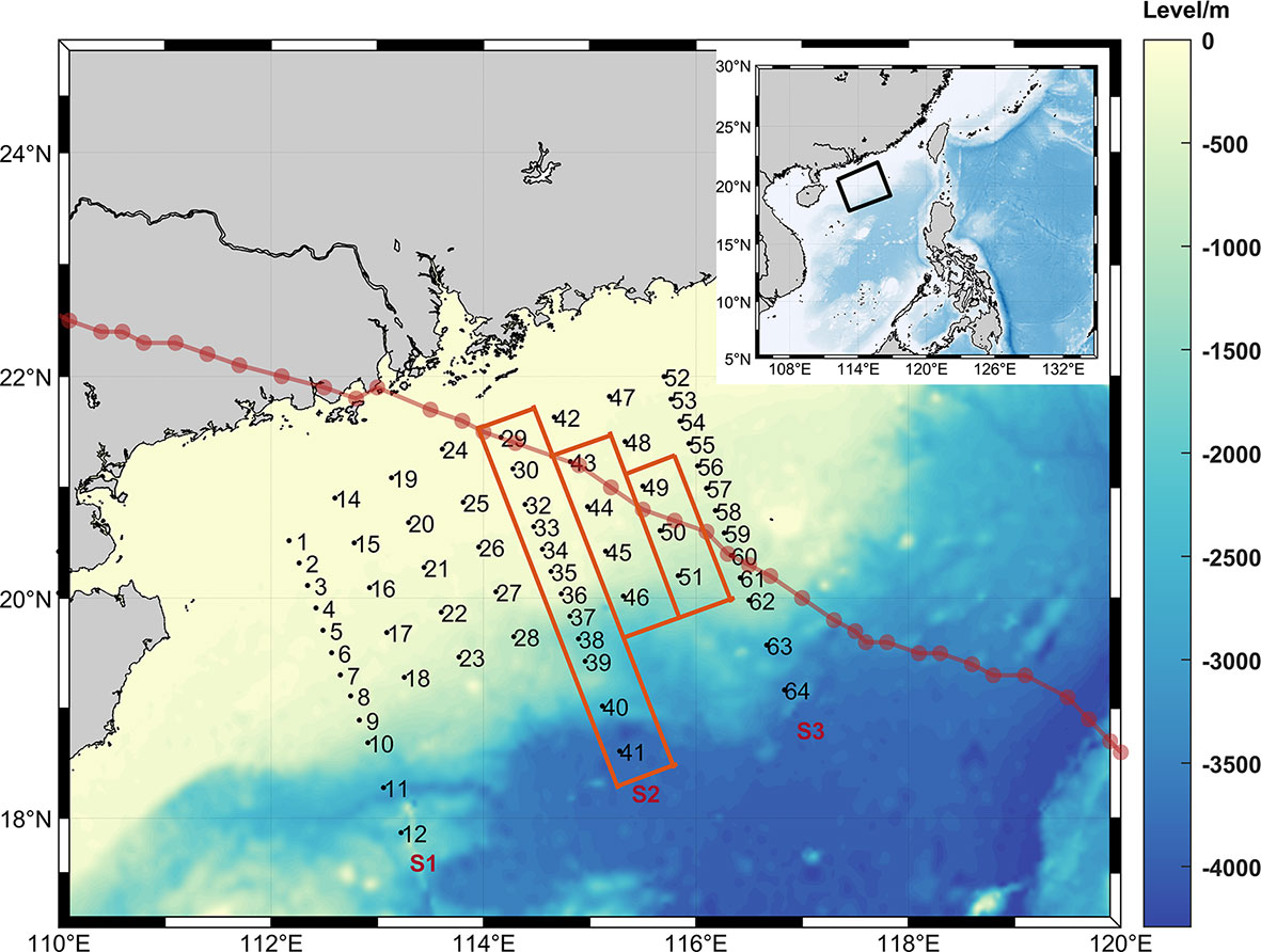
Figure 1 The study area in the SCS. The black dots and numbers are the sampling stations overlaid over topography. The 3 red boxes mark stations surveyed after the typhoon. The three long sections are S1, S2, and S3 from west to east, where S2 is the section investigated after the typhoon. The dark red solid line and dots are the path of the typhoon.

Sampling Methods

Temperature, salinity, and chlorophyll were measured by an SBE 911plus CTD (Seabird Electronics Inc., Bellevue WA, USA). The abundance and size structures of plankton were measured by an LOPC, which employs optical technologies to count and measure all particles between 0.1 and 35 mm passing through the light path in the sampling tunnel (7×7 cm wide) at 2 Hz (Herman, 2004). Compared with traditional biological sampling methods, an LOPC provides not only plankton data with high spatial-temporal resolutions but also the convenience to be deployed on various platforms such as a rosette water sampler or towed vehicle (Espinasse et al., 2018). In this survey, the LOPC was mounted on a rosette water sampler with a CTD. To avoid the effects of the rosette and CTD frames, only the data collected during the downcast are used. The counts of particles in size bins were recorded by the LOPC and data were downloaded after the instrument was recovered to the deck at each station. The size range of particles measured by an LOPC between 0.1 and 35 mm is primarily composed of mesozooplankton, microzooplankton, larger-sized phytoplankton, detritus, marine snow, and fecal particles (Espinasse et al., 2018; Zhang et al., 2019).

Data Processing

Water Column Vertical Structure

Brunt-Väisälä frequency (s⁻²) was applied to quantify the stratification, which is given by:

$\begin{array}{ll}{N}^2=-\frac{g}{\rho }\frac{\partial \rho }{\partial z},& (1)\end{array}$

where g is the acceleration constant of gravity (9.8 m s⁻²), ρ is the density (kg m⁻³), and z is the vertical axis (m). The smaller Brunt-Väisälä frequency indicates smaller density gradient and weaker stratification, and vice versa, indicating strong water column stratification.

Zooplankton Abundance and Biovolume Measured by LOPC

The downcast profile data were used for our analyses because the CTD-LOPC was lowered at a relatively stable speed without stopping for water sampling during the downcast. At each selected station, LOPC data were collected over the full water depth. During the data processing, the data down to 5 m below the sea surface were removed to avoid interference of bubbles in zooplankton measurements. The counts of particles largely depend on the volume of seawater passing through the instrument window during each sampling interval. In this study, we used the area of the opening multiplied by the depth change within the sampling time (0.5 s) as the sampling volume. The particle concentration was calculated by the particle count normalized by the sampling volume. In order to avoid repeated particle counting in strong wave conditions, the LOPC data with a depth increment of less than 0.1 m was deleted, considering the lowering speed of a CTD-LOPC of approximately 1 m s⁻¹ (Espinasse et al., 2018).

LOPC data are divided into single-element plankton (SEP) and multi-element plankton (MEP). SEP measures particles with size smaller than 1.8 mm. The instrument only records their counts and sizes in 128 size bins between 0.1 and 1.8 mm. MEP measurements count particles with body sizes greater than 1.5 mm, and record the shape of a MEP particle in addition to their counts (Herman, 2004). The particle size of a MEP particle can be calculated by a known formula and digital sizes (DS) in MEP elements (Checkley et al., 2008). It should be noted that the estimation of equivalence sphere diameter (ESD) ignores the shape of MEP particles.

$\begin{array}{ll}ESD=a_1+a_2{\displaystyle \sum DS}+a_3{\displaystyle \sum D{S}^2}+a_4{\displaystyle \sum D{S}^3},& (2)\end{array}$

where ∑DS is the sum of DSs in a MEP element, a₁ = 0.1806059, a₂ = 2.54589 × 10^-4, a₃ = -1.0988 × 10^-9, and a₄ = 9.54 × 10^-15.

In addition, the shape information of MEP could be used to calculate the transparency of the particles (Checkley et al., 2008; Basedow et al., 2013; Espinasse et al., 2018). The attnuation index (AI) was calculated as follows:

$\begin{array}{ll}AI=\frac{1}{\left(n-2\right)\times maxDS}{\displaystyle {\sum }_{i=2}^{n-1}D{S}_i},& (3)\end{array}$

where n is the number of elements and maxDS is the maximum DS of a MEP when it completely occludes a diode element. Thus, the closer the AI is to zero, the more transparent the particle is (Espinasse et al., 2018). We only retained the particles with AI > 0.4, by which non-zooplankton particles were excluded, such as marine snow or aggregates (Checkley et al., 2008; Gaardsted et al., 2010; Basedow et al., 2013; Basedow et al., 2014). Therefore, all SEPs and MEPs (AI > 0.4) were included in the measured data. At the same time, we also removed the incoherent M sequences (i.e., sequences manifested as incoherent sequence numbers of occluded elements). Studies have shown that when the particle concentration in seawater is extremely high (>10⁶ counts m⁻³), the instrument may record multiple particles as one when they passed through the laser array at the same time (Schultes and Lopes, 2009; Basedow et al., 2014).

After averaging LOPC concentrations at every 5-m depth interval, plankton concentrations of different size bins were obtained at each station. According to their sizes and concentrations, we estimated the zooplankton biovolume for different sizes within the LOPC size range. In this study, the biovolume was calculated based on the sphere volume formula instead of the ellipsoid volume formula as in the other studies. Not only are the zooplankton species measured in different shapes, the directions of the particles passing the LOPC tunnel are also uncertain. Assuming that particles passing through the tunnel are oriented randomly, this assumption is statistically equivalent to the ESD and the sphere volume formula based on ESD. By doing this, the data processing avoids any subjective hypothesis of ratios of major to minor axis for ellipsoid volume formula. All data are processed using internal programs developed by MATLAB software (MathWorks Company, USA).

Biological Volume Spectrum

The plankton size spectrum, also called size distribution, is a distribution curve between the size of the plankton and the biomass in the corresponding size interval. In order to obtain a size spectrum independent from sizes of size intervals, a normalized size spectrum is used by normalizing the biomass in a size bin by its size intervals (Platt and Denman, 1977). In recent years, scientists have developed several measures to represent the size of a plankter, such as body ESD, biovolume, dry weight, wet weight, and carbon content (Zhou et al., 2010a). In this study, we use the biovolume as the body size and biomass in a size interval. The size-dependent concentration data of zooplankton between 0.1 and 35 mm were integrated into 50 particle biovolume bins with an equal spacing based on the logarithmic scale. Then, the biomass in each biovolume bin was divided by the biovolume bin interval in order to obtain the normalized biovolume spectrum (Platt and Denman, 1977), i.e.,

$\begin{array}{ll}b=\frac{Biovolume concentration \left(m{m}^3/m^3\right) in the size bin \left(w,w+\Delta w\right)}{The size bin interval \left(\Delta w,m{m}^3\right)} \left(m^{-3}\right),& (4)\end{array}$

where b is normalized biovolume spectrum (NBVS), biovolume is in mm³, water volume filtered is in m³, w is the size of the individual plankton in mm³, and Δw is the interval of each particle size bin in mm³. The median value in each particle size class is used to represent the biovolume size of this size bin. In the double logarithmic coordinates, we apply the least square method to fit the biological volume spectrum to a straight line, that is

$\begin{array}{ll}log\left(b\right)=\beta +\alpha log\left(w\right),& (5)\end{array}$

where β is the intercept and α is the slope of the line known as the slope of an NBVS. However, the intercept β is the value of log(b) when log(w) is zero or w is the unit. The intercept is determined by both the slope and the distance of measurements away from the unit (Gómez-Canchong et al., 2013). To avoid the distance from the unit, the intercepts of log(b) at the midpoint of the log(w) size range measured were used as suggested by Daan et al. (2005). Another advantage of using the intercepts at the middle of the log size range is that this intercept is independent of the slope and is more realistic to represent the total abundance of the plankton community (Sprules et al., 2016).

Results

Hydrography

The sea surface temperature and salinity distributions show a large-scale eddy with cold and salty water center at approximately 20.75°N and 114.7°E (Figure 2). During the survey, a typhoon passed by the study area. This lower temperature and high salinity center could be caused by either wind mixing or a large-scale eddy with upwelling. The surface temperatures at those stations (stations 29–41, 43–46, and 49–51) surveyed after the typhoon were about 1.5°C lower than that of other stations. The surface salinity was between 32 nearshore and 34 off-shelf. After the typhoon, the temperature and salinity of the water column changed due to mixing of the 0–50 m water column (Figure 3). The low salinity water was a mixture between freshwater runoffs and nearshore water. The salinity values at most shelf and off-shelf stations were about 33.5, while the surface salinity at the sites after the typhoon were about 33.8, presumably due to mixing and Ekman pumping.

FIGURE 2

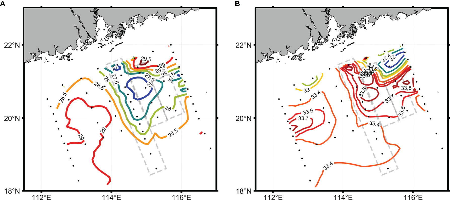
Figure 2 Sea surface temperature (SST, °C) (A) and sea surface salinity (SSS) (B) in the study area. The gray dashed boxes are the stations sampled after the typhoon.

FIGURE 3

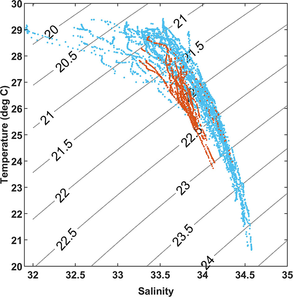
Figure 3 T–S diagram of 62 stations from surface to 50 m depth. Blue solid points are water columns before the typhoon and orange solid points are water columns affected by the typhoon.

In summer, the water column was stratified in the northern SCS (Figure 4). The mixed layer was shallower than 30 m, and the thermocline and halocline were hydrostatically stable in the upper 50 m. The stratification of the water column varied between shelf and off-shelf regions and also before and after the typhoon. The water column on the shelf was well stratified before the typhoon arrived (Figures 4A, C). After the typhoon, the shallow water columns on the shelf were mixed (Figure 4B). On and off slope, the water columns were deep enough to remain stratified though the mixed layers deepened (Figure 4). Several bulges of isotherms and isohaline on transects S1–3 appeared near the 200-m isobath. At these stations, the salinity of the mixed layer was higher than those of the surrounding stations and the temperatures were lower than those of the surrounding stations. The salinity was increased, the halocline was disturbed, and the stratification strength was weakened.

FIGURE 4

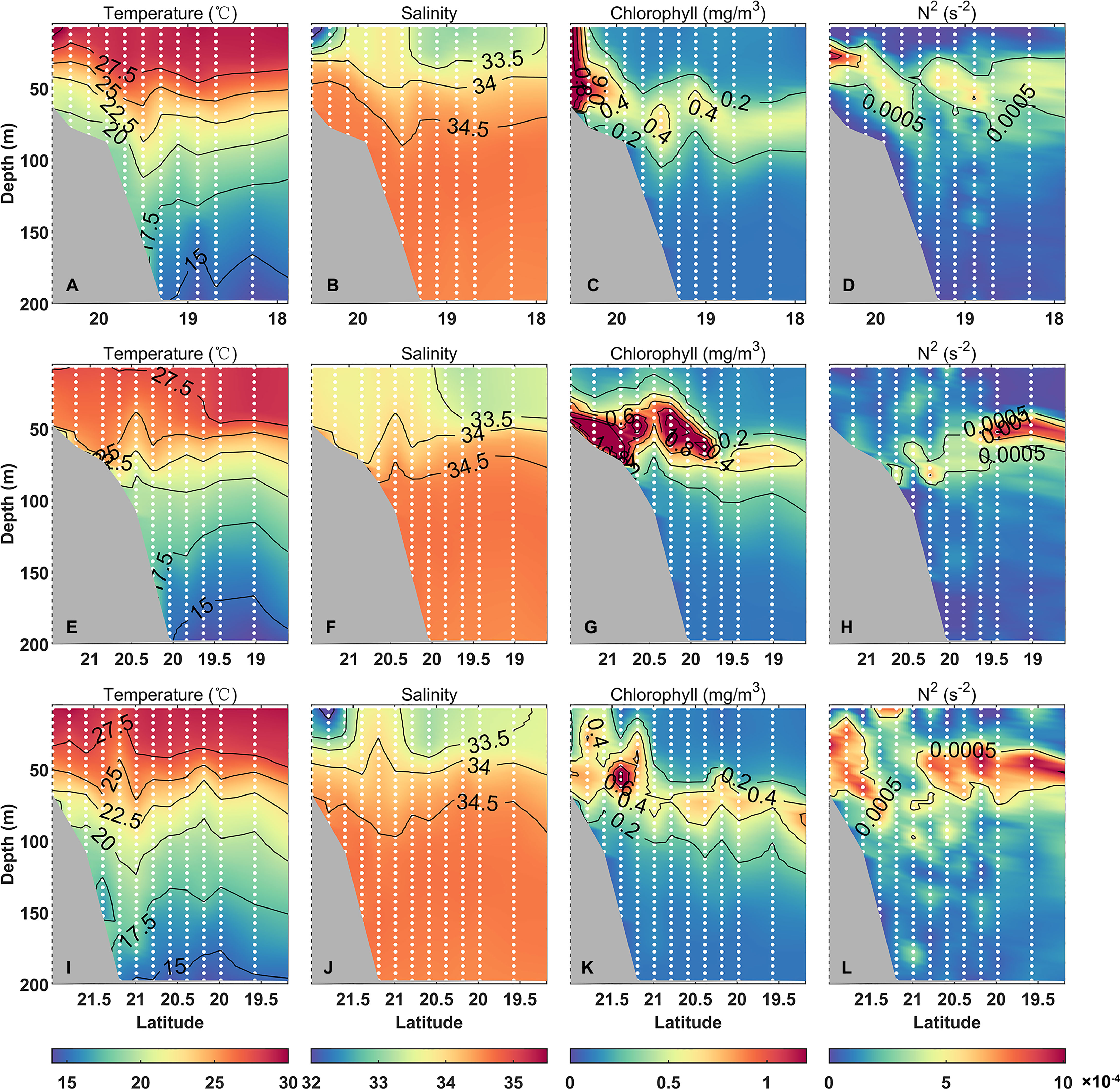
Figure 4 Three transects [S1: (A–D), S2: (E–H), S3: (I–L)] of temperature (°C, left panel), salinity (the second panel), chlorophyll concentration (mg/m³, the third panel), and Brunt-Väisälä frequency (s⁻², right panel). The solid white dots are the positions of the sites.

To measure the degree of water column stratification, Brunt-Väisälä frequency (N²) was computed along transects S1, S2, and S3 (Figure 4). The N² maximum was between 25 and 85 m, shallower on the shelf region by about 30 m, and deeper in the off-shelf area by about 50 m. Because the water column on transect S2 was affected by the typhoon, the N² maximum was at about 85 m at stations 33 and 35.

Chlorophyll Distribution

In summer 2018, the chlorophyll maximum in the northern SCS appeared in the subsurface layer, with a depth of about 50–75 m (Figure 4). The subsurface chlorophyll maximum (SCM) in the slope region was deeper than that of the shelf, and the deepest at station 64 was at approximately 82.5 m. The average chlorophyll concentration within the shallow water column at 200 m in the northern SCS was 0.36 mg m⁻³, measured by a calibrated fluorometer except for the abnormal value of station 1. The average chlorophyll concentration in the water column at station 32 affected by the typhoon was the highest, 0.84 mg m⁻³, and the concentration at station 11 at the slope area was 0.18 mg m⁻³, which is the station with the lowest chlorophyll concentration. The chlorophyll concentrations of the nearshore shelf stations were generally higher than those of the off-shelf slope regions. The chlorophyll concentrations of the stations after the typhoon were systematically higher than those of the other stations surveyed before the typhoon. The maximum chlorophyll concentrations on the shelf were generally greater than 1.0 mg m⁻³. On the shelf, the pycnocline and SCM co-occurred in the shallow-water region, while the deep-water shelf region has the SCM in the lower half of the pycnocline.

Spatial Distributions of Plankton

The average abundance of plankton in the upper 200 m was 10.74×10⁴ ind. m⁻³ (Figure 5). The maximum abundance was 33.58×10⁴ ind. m⁻³ at station 2 near the coast while the lowest abundance was 2.31×10⁴ ind. m⁻³ at station 23 in the continental slope area. At the same time, the average biomass in the SCS was 1.21×10³ mm³ m⁻³ (Figure 5). The maximum biovolume was 17.98×10³ mm³ m⁻³ at station 30 near the coast while the lowest biovolume was 0.13×10³ mm³ m⁻³ at station 28 in the continental slope area. The plankton abundance (p < 0.01) and biovolume (p < 0.01) in the continental slope were generally lower than those in the shelf region. There were significant changes in abundance (p < 0.05) after the typhoon while the changes in biovolume were not significant (Supplementary Table 1).

FIGURE 5

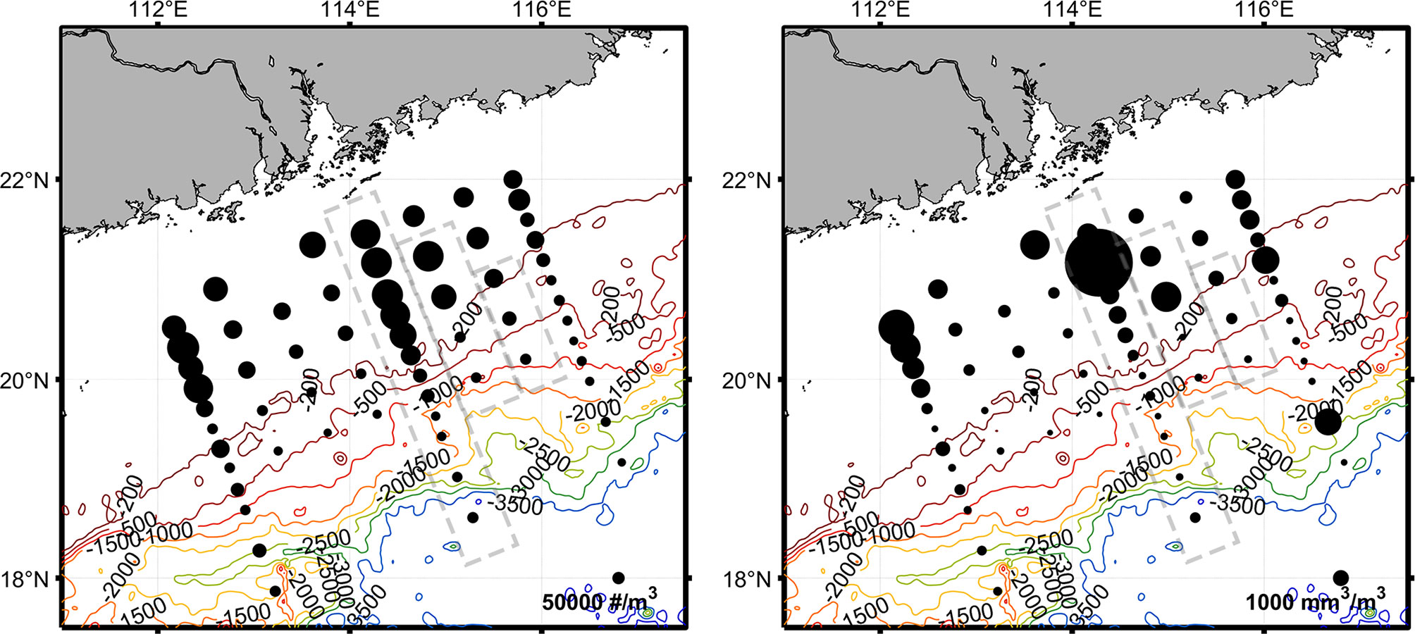
Figure 5 The water column average of plankton abundance distribution (#/m³, left panel) and biovolume concentration (mm³/m³, right panel) in northern SCS. The gray dashed boxes are the stations sampled after the typhoon.

The zooplankton distributions of 5 different size groups are shown along the 3 transects (Figure 6). The plankton biovolume concentrations were higher in the upper 100 m than that at depth. The abundance and biovolume concentrations of zooplankton near the pycnocline were the highest (Figure 6). Especially in the off-slope region, the biovolume maximum layer of small-size plankton was co-occurring well with the pycnocline, while the distribution of large-size plankton was less correlated with the pycnocline. Before the typhoon, the biovolume (r² = 0.52, p < 0.01) and abundance (r² = 0.70, p < 0.01) in the off-shelf region were aggregated near the density discontinuity and more dispersed in the shelf region (biovolume: r² = 0.19, p < 0.01; abundance: r² = 0.28, p < 0.01). At the stations on the shelf on transect S2 affected by the typhoon, the water columns were fully mixed, and plankton was evenly distributed in the water column without aggregations (biovolume: r² = −0.32, p < 0.01; abundance: r² = −0.24, p < 0.05) (Supplementary Table 2).

FIGURE 6

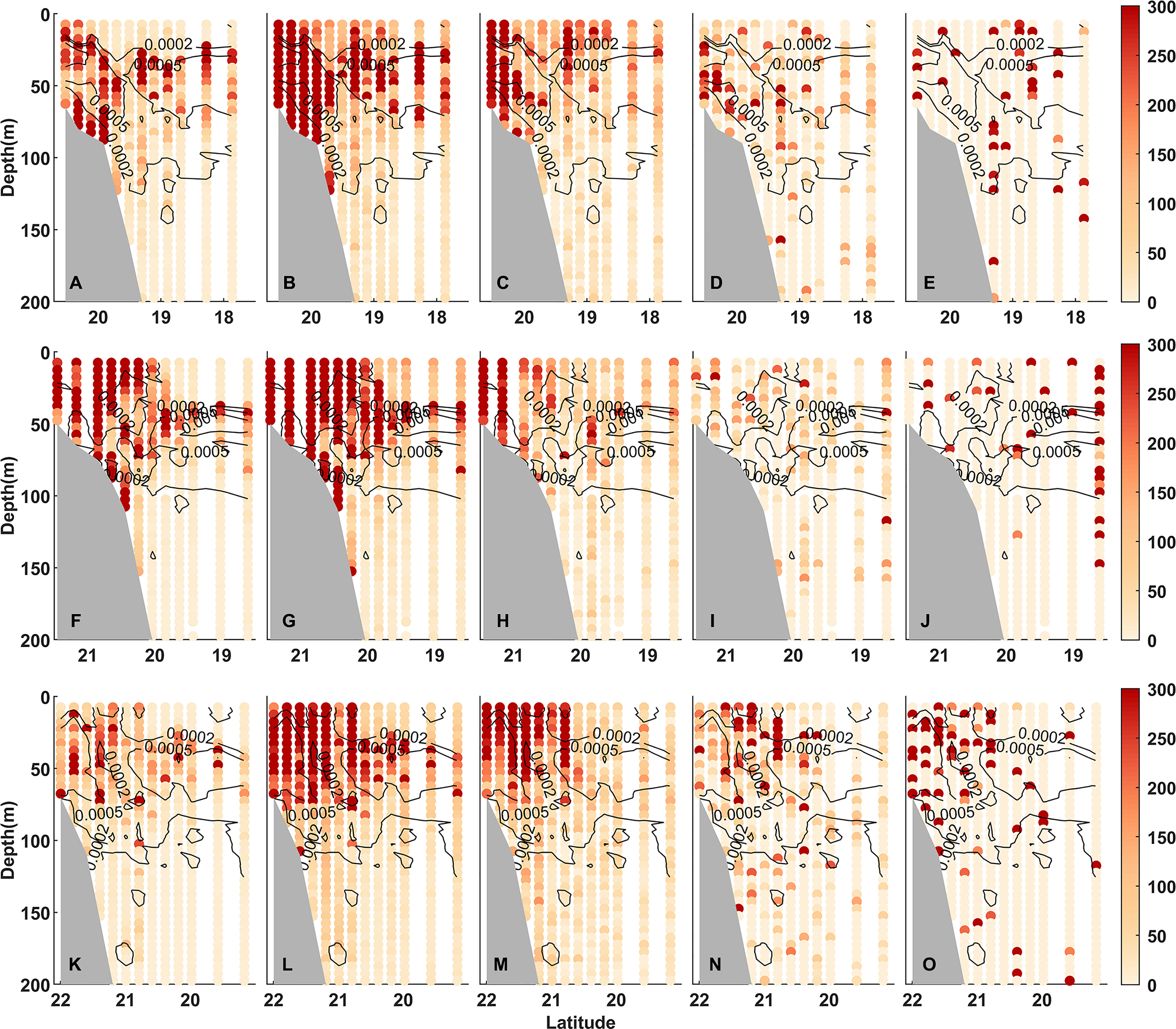
Figure 6 Contours are Brunt-Väisälä frequency (s⁻²) and solid circles are biovolume (mm³/m³) of five size groups [(A, F, K) 0.1–0.2 mm, (B, G, L) 0.2–0.5 mm, (C, H, M) 0.5–1.0 mm, (D, I, N) 1.0–2.0 mm, and (E, J, O) >2.0 mm] along transect S1 (upper panel), S2 (middle panel), and S3 (lower panel).

The Slope and Intercept of Biovolume Spectrum

The slopes of the size spectra along these 3 transects varied between −0.4 and −1.2 (Figure 7). The slope showed obvious differences between shelf and off-shelf regions (p < 0.01). At the same time, the intercepts exhibited similar variations to the slopes, ranging from 2 to 4.5 with the regional differences (p < 0.01) (Supplementary Table 1). Regional differences in slopes and intercepts of NBVS were reflected in the variations in the water column. In the off-shelf region, the slopes and intercepts presented significant negative correlation (r² = −0.61, p < 0.01) and positive correlation (r² = 0.67, p < 0.01) with stratification, respectively. In contrast, the correlations were weaker on the shelf (slope: r² = −0.14, p>0.05; intercept: r² = 0.26, p < 0.01) (Supplementary Table 2).

FIGURE 7

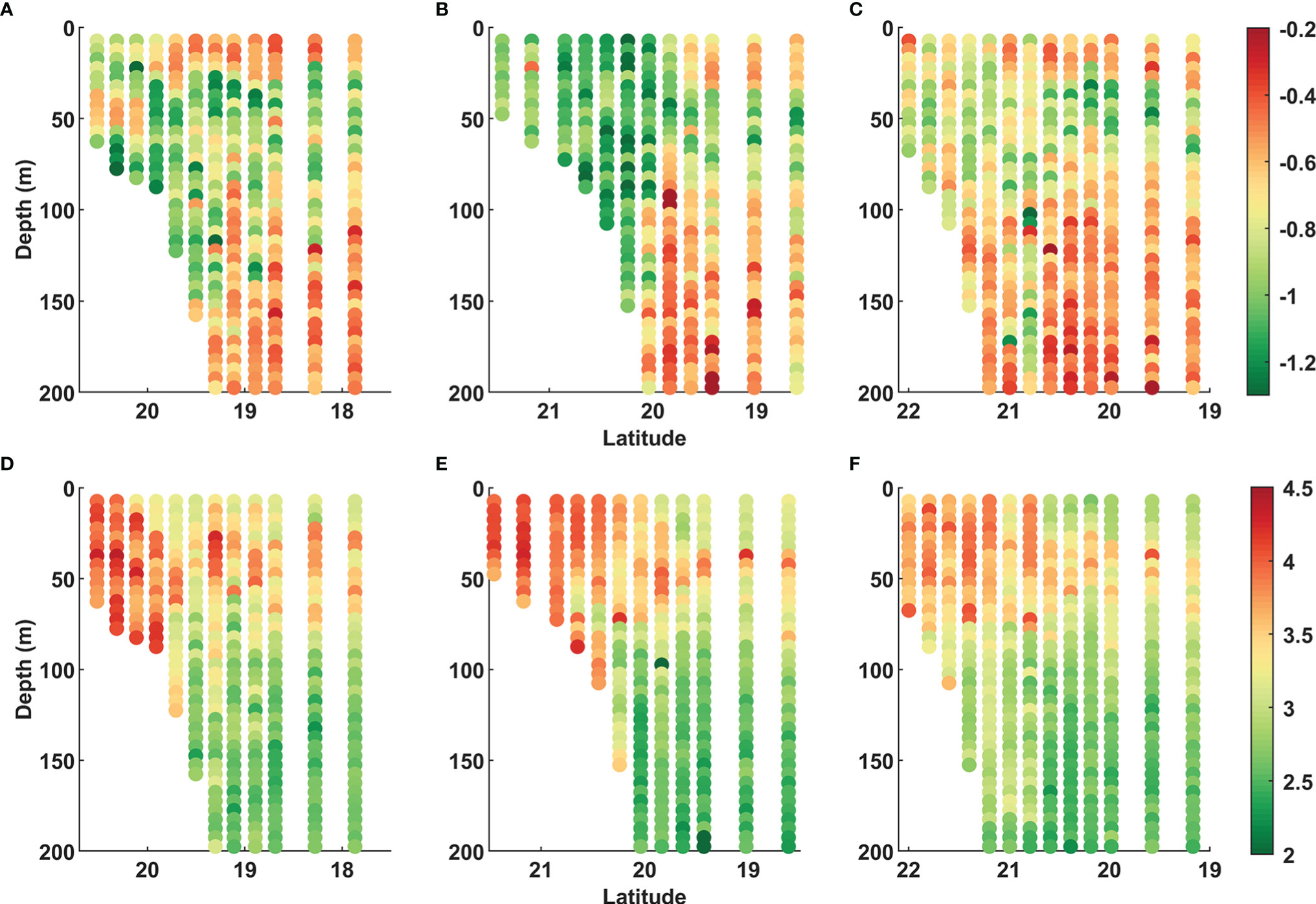
Figure 7 Slopes (A–C) and intercepts (D–F) of NBVS in transect S1 (left panel), S2 (middle panel), and S3 (right panel).

The stations of the three sections were divided into four groups according to measurements before and after the typhoon, and regions on shelf and off the shelf. The slopes and intercepts of NBVS were computed, and the differences and variations in slopes and intercepts were analyzed. The stratification in the off-shelf area was stronger than that of the shelf, and the slopes and intercepts exhibited strong vertical variations (Figure 8). In the off-shelf area, the slopes were flatter between −0.4 and −0.6 in the upper layers (0–30 m), steeper between −0.9 and −1.1 in the pycnocline and SCM (30–80 m), and flattest in the deep-water column (>80 m) (Figure 8), while the slopes in the shelf area varied by approximately −0.8 with less variations in the vertical. In the shelf region after the typhoon, the strong mixing caused the destratification leading to a uniformly mixed water column. The vertical variations of the slopes were small, while the slopes were significantly steeper than those before the typhoon (p < 0.01, Supplementary Table 1). The intercepts of NBVS were the highest (approximately 4.0) at the surface and decreased with depth in the shelf area both before and after the typhoon. In the off-shelf region, the curves of buoyancy frequency indicated that the mixed layer was deepened by typhoon steering. The corresponding patterns between stratification structure, slopes, and intercepts remained consistent with those before the typhoon. The intercepts were approximately 3.0 in the mixed layer, and increased to a maximum (near 4.0) at the pycnocline and decreased to approximately 2.5 at 200 m.

FIGURE 8

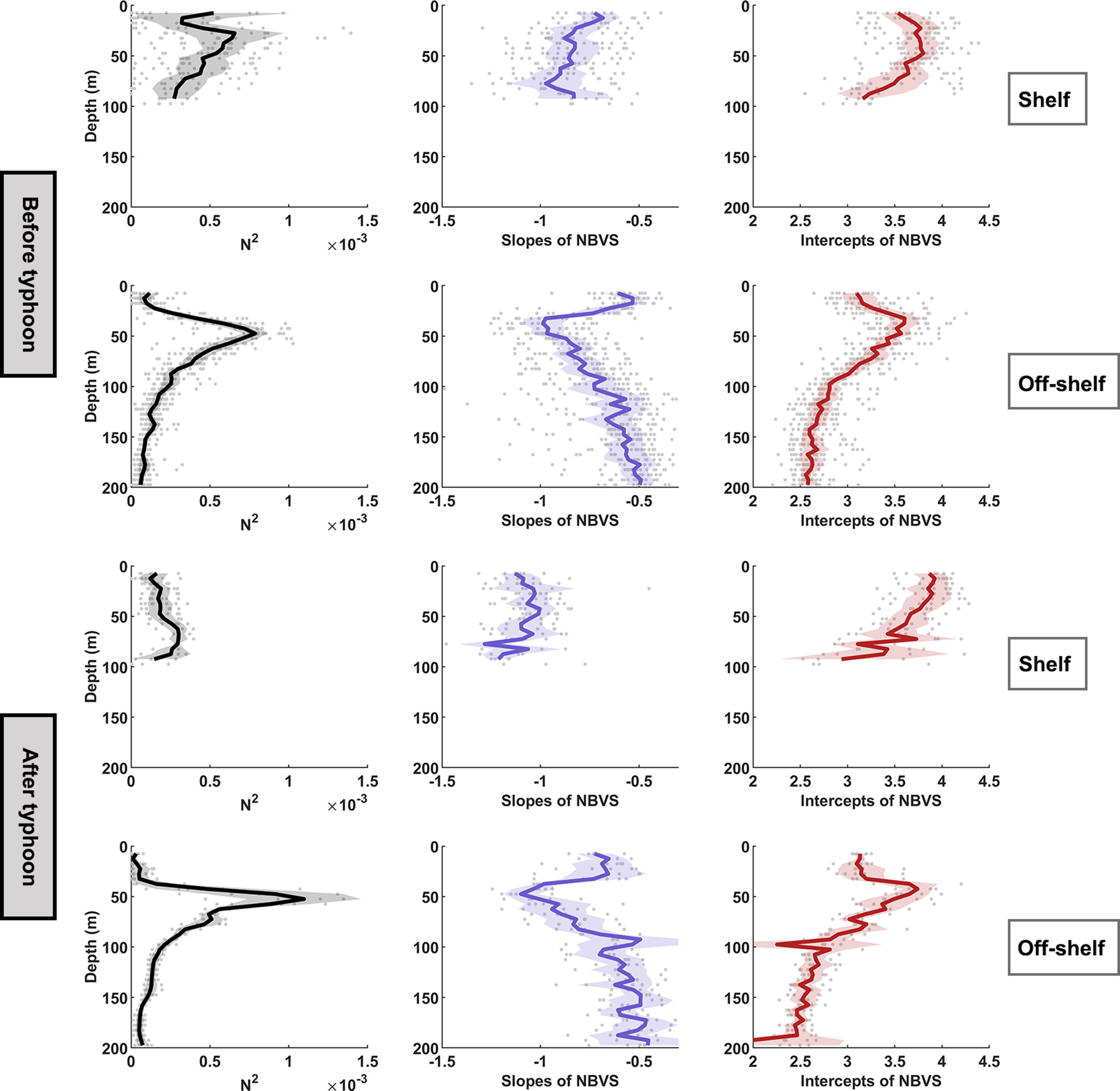
Figure 8 Variations in N² (s⁻²), the slopes of NBVS, and the intercepts of NBVS with depth in the shelf and off-regions during pre-typhoon and post-typhoon periods. Dark thick solid lines are averages, light transparent filled areas are the 95% confidence intervals, and the light gray points are the measured data within the groups.

To compare the NBVS between different layers and to understand the impact of the typhoon, we conducted statistical analysis of the slopes and intercepts of the three vertical layers before and after the typhoon (Figure 9). These three layers were the mixed layer (0–30 m), the subsurface layer (30–80 m) including pycnocline and SCM, and the deep layer (>80 m). After the typhoon on the shelf, the slopes in these three layers became steeper, especially in the upper layer. Although the slopes in the upper and subsurface layers in off-shelf regions also became steeper, the changes of these slopes were less than those on the shelf. The slopes in the deep water were even flatter, that is, less affected by the typhoon. The intercepts on the shelf increased in the upper layer and decreased in the deep water after the typhoon. The intercepts in the subsurface layer including SCM in the off-shelf areas were the highest in the vertical before and after the typhoon. The intercepts in the mixed layer and subsurface layer were not significantly changed by the typhoon effect (Figure 9).

FIGURE 9

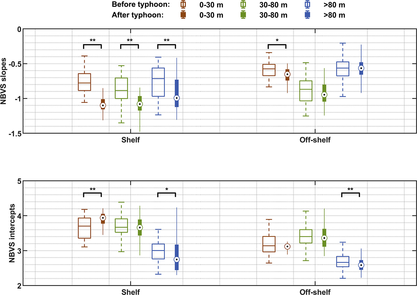
Figure 9 The slopes (upper panel) and intercepts (lower panel) of each layer in the shelf and off-shelf regions before and after the typhoon. The hollow bars are the averages before the typhoon, the solid bars are the averages after the typhoon, and the short lines or circles in the boxes are the medians. Each data group before and after the typhoon was tested by the Mann–Whitney U test. The test results are marked above the short black lines. **p < 0.01, *p < 0.05.

Discussion

Ground Truth of LOPC Data

The design and purpose of an LOPC are not made to distinguish living or nonliving particles such as plankton and marine snow during the sampling process. The ground truth relies on other sampling methods such as plankton net tows and camera systems (Wiebe and Benfield, 2003). A number of studies have tried to separate plankton and aggregates using different reference parameters or mathematical models (Jackson and Checkley, 2011; Petrik et al., 2013; Trudnowska et al., 2018). AI is a parameter calculated based on shape information recorded by LOPC, using it to separate very transparent aggregates or marine snow, applied in many studies and proven to be effective (Checkley et al., 2008; Gaardsted et al., 2010; Basedow et al., 2013; Basedow et al., 2014; Wiedmann et al., 2014). Particles with AI < 0.4 were excluded, which was a stringent condition (Gaardsted et al., 2010; Basedow et al., 2013). Although it ensured that most of the transparent aggregates were separated from zooplankton, it was also possible that some transparent zooplankton such as hydrozoans were excluded. Based on previous results, the proportion of hydrozoans in the investigation area was small, so we still used 0.4 as the differentiation threshold (Zhang et al., 2019).

In order to verify biomass measurements by an LOPC, samples from other plankton sampling instruments were used for comparison (Gaardsted et al., 2010; Basedow et al., 2013; Marcolin et al., 2015a; Kydd et al., 2018). In this study, we used the abundance and biomass data of certain species collected by plankton nets from the previous investigations in the northern SCS for interpreting plankton species vs. abundances and sizes of LOPC measurements. Between an LOPC size range and specific plankton species, the comparative results of biomasses measured by an LOPC and net tows are in the same order of magnitude (Table 1). The values from LOPC measurements are typically higher than that of net tows (Schultes and Lopes, 2009; Gaardsted et al., 2010; Watkins et al., 2017). Zooplankton can easily avoid a net or be squeezed out through the mesh of a net.

TABLE 1

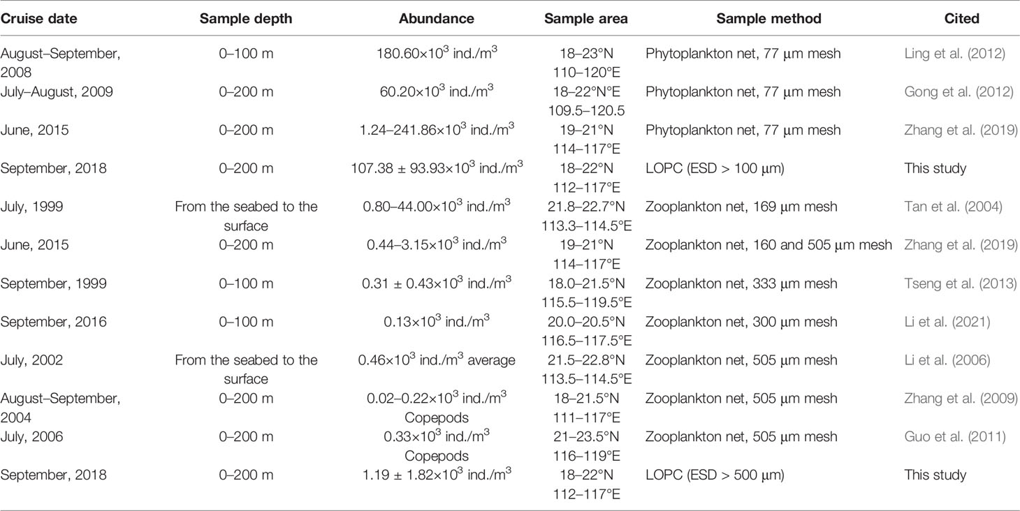
Table 1 Data about plankton abundance from previous studies and this study in different size groups in the northern SCS.

The plankton community compositions were analyzed based on the taxonomic information for a set of size intervals previously investigated using live zooplankton samples collected by plankton nets in the northern SCS. Plankton smaller than 200 μm are primarily composed of diatoms like Rhizosolenia, Coscinodiscus, and Chaetoceros as well as dinoflagellates such like Ceratium (Zhang, 2016). Although microplankton such as ciliates are an important part of zooplankton smaller than 200 μm feeding on picophytoplankton, many studies indicate that their abundances are still low compared with that of phytoplankton in the same size range (Strom, 2002; Calbet and Landry, 2004; Leising et al., 2005). Some large phytoplankton (Rhizosolenia and Chaetoceros) and copepods dominate in the 200- to 500-μm size range (Zhang, 2016; Zhang et al., 2019). Zooplankton larger than 500 μm is primarily composed of copepoda, accounting for 70% of the total zooplankton, of which copepoda dominated in the 0.5–1.0 mm group; in the 1.0–2.0 mm size class, copepoda and Chaetognatha were the main components, and the larger than 2.0 mm group included Chaetognatha, Euphausiacea, and copepoda (Zhang et al., 2019). Copepods are the most dominant component of zooplankton in the northern SCS, and their grazing rate of phytoplankton reaches 20% (Chen et al., 2015). Picophytoplankton are the dominant population of phytoplankton in the northern SCS, which are more frequently consumed by microzooplankton (Calbet and Landry, 2004; Chen et al., 2013; Pan et al., 2017). Copepods may not be able to directly ingest these small algae, making carnivorous and omnivorous zooplankton important links between trophic levels (Chen et al., 2017).

Pycnocline and Biomass Maxima

It has been observed that zooplankton are concentrated within the pycnocline because aggregates and marine snow are accumulated in the pycnocline (Herman, 1983; Harris, 1988; Möller et al., 2012; Trudnowska et al., 2016). Previous studies have found that the accumulation of aggregates or marine snow in the pycnocline is caused by a rapid decrease in settling speed due to the steep density gradient (Möller et al., 2012; Espinasse et al., 2018). In such a case, the SCM is typically above the pycnocline so that dead phytoplankton cells or exopolymers are forming marine snow while sinking into the pycnocline where they accumulate (Alldredge and Silver, 1988; Turner, 2002; Espinasse et al., 2018; Briseno-Avena et al., 2020). In this study, the SCM was generally located below the pycnocline so that the marine snow or aggregates will sink deeper into the ocean without being stopped by any density gradient. There are possibilities of fecal pellets or debris falling into the pycnocline attracting zooplankton to aggregate. As the results showed, most of the excluded particles (AI < 0.4) were concentrated near the pycnocline (Supplementary Figure 1). One thing noticeable was that at some stations in this study, the maximum biovolume layer mismatched the SCM layer. Biovolume maxima are typically above the SCM. It is well known that due to photo quenching, the SCM may not be the biomass maximum. Our findings are consistent with the relationship between photo quenching and SCM. This phenomenon that zooplankton biovolume maxima are above the SCM has also been found in other sea areas, but detailed reasons for this mismatch are not clear (Herman, 1983; Roman et al., 1986; Harris, 1988; Briseno-Avena et al., 2020).

Size-Dependent Distribution of Zooplankton

The results on size–distribution relationships of zooplankton reveal the trend that smaller plankton is greatly associated with stratification while larger plankton tend to be less associated with stratification (Figure 6). In the size range of less than 500 μm, there are primarily composed of phytoplankton and small zooplankton. Both phytoplankton and small zooplankton have very limited mobility. Their vertical distributions are dependent on density differences between plankton and ambient water and mixing. At the pycnocline, the rapid density increase leads to an accumulation of biomass. In the pycnocline, it is also difficult for the small-sized zooplankton, such as ciliates, to cross the stratification and move vertically because of their weak capability to overcome buoyancy forces. Trudnowska et al. (2016) reported that 0.3- to 0.8-mm particles aggregated at density discontinuities to facilitate their retention of their location. Larger zooplankton, such as copepods or krill larvae, and have strong swimming ability. They can move vertically in the water column by controlling their buoyancy, possessing a competitive advantage for food (Yayanos et al., 1978; Pond and Tarling, 2011). Overall, the biovolume concentrations of large particles in the deep water were reduced less than those of small particles, indicating their capabilities of grazing and swimming.

Regional Variations in Plankton Community

A normalized size spectrum provides two important parameters, slope and intercept, with an assumption of linearity (Platt and Denman, 1977; Zhou and Huntley, 1997; Zhou, 2006). The intercept is interpreted as total abundance while the slope is interpreted as the community size structure. The variations of slopes and intercepts in the water column exhibited regional differences. In the off-shelf surface water, the primary productivity and biovolume concentrations (smaller intercepts) in the surface water were lower due to the oligotrophic condition, and the slopes of NBVS were flatter as an indicator of lower small-sized plankton proportion. Total abundance was highest in the off-shelf SCM. The slopes of NBVS were steeper, indicating not only more small, lower trophic particulate organic matter available to feed grazers but also lower energy transfer efficiency or fewer trophic levels (Zhou, 2006; Atkinson et al., 2020).

In contrast to the persistent and stable stratification in the off-shelf area, the shelf region was affected by various factors such as upwellings, terrestrial runoffs, and sediment resuspensions. The size structures in the water columns exhibited homogeneity. Total abundance was high in both the mixed and subsurface layers, with small-sized plankton dominating the community. These implied a higher potential productivity and more herbivorous zooplankton of the entire water column on the shelf (Zhou, 2006; Trudnowska et al., 2014). Onshore–offshore variations in the abundance, predominant species, and richness of zooplankton in northern SCS have been reported (Zhang et al., 2009). Regional differences in zooplankton community size structure might be attributed to differences in phytoplankton communities. It has been indicated that microphytoplankton with high concentration on the shelf gradually shifted to picophytoplankton dominated in phytoplankton community in open sea (Dong et al., 2018). In the shelf region, small copepods increased their proportion in the community by aggregation or reproduction because they preferred to feed on microphytoplankton rather than on picophytoplankton (Calbet and Landry, 2004; Pan et al., 2017).

Effects of Typhoon

The typhoon-induced destratification was evident as well-mixed water columns on the shelf along transect S2 in Figures 4 and 8. Both the bottom of the mixed layer and SCM deepened to the sea bottom about 70 m after the typhoon. The small particle concentrations measured by the LOPC indicated high values near the bottom, implying that the SCM was related to re-suspension of settled materials (Figure 6F). The chlorophyll concentrations on the shelf increased after the typhoon. In the previous study on nutrients about the “Mangkhut” event, nutrients increased significantly (nitrate and phosphate increased by about 80% and 36%) in the shelf region due to the impact of the typhoon (Kuss et al., 2021). In the SCS, the growth of phytoplankton was limited by nitrogen and the increase of nitrate was considered to be the key precondition for the blooms in oligotrophic water (Pan et al., 2017; Liu and Tang, 2018). After the typhoon, the oligotrophic algae (mainly picophytoplankton) in the oligotrophic waters decreased significantly, and the microphytoplankton became the dominant species (Chen et al., 2009).

The stirring of the typhoon caused the steeper slopes and the higher intercepts of the upper layer on the shelf (Figure 9). The enhanced abundance in the upper layer should be a result of the nutrients supplemented by the typhoon process promoting the growth and reproduction of phytoplankton and thus small zooplankton reflecting a positive change as a result of additional food. The doubling rates of phytoplankton and zooplankton are typically 2 to 10 days in the size range of our study (Hirst and Bunker, 2003; Zhou et al., 2010b; Lin et al., 2013). The time difference between the typhoon and sampling at shelf stations 29–34 was approximately 4–5 days. The steeper slopes might imply a decrease in trophic transfer efficiency or an increase in herbivorous species as the phytoplankton community was altered (Zhou, 2006; Trudnowska et al., 2014; Atkinson et al., 2020), whereas the decrease in abundance in the layer deeper than 80 m may be due to the mixing, accelerating the settling of large-sized zooplankton, resulting in steeper slopes.

We took it for granted that mixing would have a positive effect on the abundance of the off-shelf region, but this did not turn out to be the result. The abundance of plankton at the off-shelf sites presented little difference from before, which was consistent with the previous results. Kuss et al. (2021) have reported that the changes of nutrients and POC in the off-shelf area after the typhoon were not significant or even decreased in this typhoon event. Therefore, in the continental slope area, the typhoon process did not promote plankton reproduction. Along with the deepening of the mixed layer, the larger sinking flux of large-sized plankton may have reduced their proportion of the community, resulting in the steeper slopes of NBVS. Previous studies have reported differences in nutrient and phytoplankton responses between shelf and off-shelf regions. Nutrients on the shelf were more easily elevated to the surface than those on the off-shelf (Fogel et al., 1999). After the typhoon, large-sized phytoplankton increased more in the shelf region than in the open sea (Ma et al., 2021). These differences were also reflected in the zooplankton community and NBVS.

Summary

The distributions of plankton NBVS in the northern SCS were strongly associated with shelf and off-shelf regions in the horizontal direction, and stratification, SCM, and depth of the water column in the vertical direction. In the shelf region, the primary production was enhanced by runoffs of nutrients and biota, and the biovolume concentrations in different size bins were higher and enhanced in SCM; the slopes of NBVS were vertically homogeneous and relatively steep, indicating a primary production dominated by the plankton community structure. In the off-shelf region under the oligotrophic condition, the biovolume concentrations of smaller plankton were featured with lower biovolume concentration and flatter NBVS in the surface water, higher biovolume concentration and steeper NBVS in SCM, and lower biovolume concentration and flatter NBVS in the deep water. Effects of mixing by typhoons on the plankton communities in the shelf and off-shelf areas can be interpreted in terms of slopes and intercepts of NBVS. The mixing steered by the typhoon changed the slope became steeper and intercept to higher for a size structured plankton community in the mixed layer and SCM, implying an increase in the proportion of small-sized plankton. In general, typhoons can enhance nutrient supply and primary production in the upper layer, resulting in high production of the plankton community. These will lead to a higher intercept and a steep slope of an NBVS. There have been few investigations on NBVS in the northern SCS due to the limitation of technical methods. Most studies on NBVS were established on the average biomass from the surface to a broad depth range covering mixed layer, pycnocline, and SCM, ignoring the changes in the vertical direction so far. This study found that the vertical variations of 2 NBVS parameters, i.e., intercept and slope, are strongly correlated with stratification, SCM, and depth.

Data Availability Statement

The raw data supporting the conclusions of this article will be made available by the authors, without undue reservation.

Author Contributions

KC and MZ designed the original ideas presented in this manuscript. KC, YZ, and JW collected the field measurements. KC and CS analyzed the LOPC data. KC wrote the manuscript. MZ, JW, YZ, and ZZ revised and improved the manuscript. All authors contributed to the article and approved the submitted version.

Conflict of Interest

The authors declare that the research was conducted in the absence of any commercial or financial relationships that could be construed as a potential conflict of interest.

Publisher’s Note

All claims expressed in this article are solely those of the authors and do not necessarily represent those of their affiliated organizations, or those of the publisher, the editors and the reviewers. Any product that may be evaluated in this article, or claim that may be made by its manufacturer, is not guaranteed or endorsed by the publisher.

Acknowledgments

This research work is funded by the International Cooperation of the National Natural Science Foundation of China (No. 41861134040), the National Program on Key Basic Research Project of China (973 Program, No. 2014CB441500), the Sino-German Cooperation in ocean and polar research-Megacity’s fingerprint in Chinese marginal seas: Pollutant fingerprints and dispersal transformation (MEGAPOL), and the National Natural Science Foundation of China (No. 41706014). JW is supported by MEGAPOL with the contract number BMBf (03F0786A) Federal Ministry of Education and Research. MZ would like to acknowledge the support from the captains and crew of R/V Haiyang Dizhi 10. KC would like to acknowledge Shuangzhao Li and Zhiqiang Su for their help in data collection.

Supplementary Material

The Supplementary Material for this article can be found online at: https://www.frontiersin.org/articles/10.3389/fmars.2022.870021/full#supplementary-material

References

Alldredge A. L., Silver M. W. (1988). Characteristics, Dynamics and Significance of Marine Snow. Prog. Oceanog. 20 (1), 41–82. doi: 10.1016/0079-6611(88)90053-5

CrossRef Full Text | Google Scholar

Atkinson A., Lilley M. K. S., Hirst A. G., McEvoy A. J., Tarran G. A., Widdicombe C., et al. (2020). Increasing Nutrient Stress Reduces the Efficiency of Energy Transfer Through Planktonic Size Spectra. Limnol. Oceanog. 66 (2), 422–437. doi: 10.1002/lno.11613

CrossRef Full Text | Google Scholar

Basedow S. L., Tande K. S., Norrbin M. F., Kristiansen S. A. (2013). Capturing Quantitative Zooplankton Information in the Sea: Performance Test of Laser Optical Plankton Counter and Video Plankton Recorder in a Calanus Finmarchicus Dominated Summer Situation. Prog. Oceanog. 108, 72–80. doi: 10.1016/j.pocean.2012.10.005

CrossRef Full Text | Google Scholar

Basedow S. L., Zhou M., Tande K. S. (2014). Secondary Production at the Polar Front, Barents Sea, August 2007. J. Mar. Syst. 130, 147–159. doi: 10.1016/j.jmarsys.2013.07.015

CrossRef Full Text | Google Scholar

Briseno-Avena C., Prairie J. C., Franks P. J. S., Jaffe J. S. (2020). Comparing Vertical Distributions of Chl-A Fluorescence, Marine Snow, and Taxon-Specific Zooplankton in Relation to Density Using High-Resolution Optical Measurements. Front. Mar. Sci. 7. doi: 10.3389/fmars.2020.00602

CrossRef Full Text | Google Scholar

Buitenhuis E., Le Quéré C., Aumont O., Beaugrand G., Bunker A., Hirst A., et al. (2006). Biogeochemical Fluxes Through Mesozooplankton. Global Biogeochem. Cycle. 20 (2), GB2003. doi: 10.1029/2005gb002511

CrossRef Full Text | Google Scholar

Calbet A., Landry M. R. (2004). Phytoplankton Growth, Microzooplankton Grazing, and Carbon Cycling in Marine Systems. Limnol. Oceanog. 49 (1), 51–57. doi: 10.4319/lo.2004.49.1.0051

CrossRef Full Text | Google Scholar

Checkley D. M., Davis R. E., Herman A. W., Jackson G. A., Beanlands B., Regier L. A. (2008). Assessing Plankton and Other Particles in Situ With the SOLOPC. Limnol. Oceanog. 53 (5_part_2), 2123–2136. doi: 10.4319/lo.2008.53.5_part_2.2123

CrossRef Full Text | Google Scholar

Chen Y. L. L., Chen H. Y., Jan S., Tuo S. H. (2009). Phytoplankton Productivity Enhancement and Assemblage Change in the Upstream Kuroshio After Typhoons. Mar. Ecol. Prog. Ser. 385, 111–126. doi: 10.3354/meps08053

CrossRef Full Text | Google Scholar

Chen Y., Lin S., Wang C., Yang J., Sun D. (2020). Response of Size and Trophic Structure of Zooplankton Community to Marine Environmental Conditions in the Northern South China Sea in Winter. J. Plankton. Res. 42 (3), 378–393. doi: 10.1093/plankt/fbaa022

CrossRef Full Text | Google Scholar

Chen M., Liu H., Chen B. (2017). Seasonal Variability of Mesozooplankton Feeding Rates on Phytoplankton in Subtropical Coastal and Estuarine Waters. Front. Mar. Sci. 4. doi: 10.3389/fmars.2017.00186

CrossRef Full Text | Google Scholar

Chen M. R., Liu H. B., Song S. Q., Sun J. (2015). Size-Fractionated Mesozooplankton Biomass and Grazing Impact on Phytoplankton in Northern South China Sea During Four Seasons. Deep-Sea. Res. Part Ii-Topical. Stud. Oceanog. 117, 108–118. doi: 10.1016/j.dsr2.2015.02.026

CrossRef Full Text | Google Scholar

Chen B., Zheng L., Huang B., Song S., Liu H. (2013). Seasonal and Spatial Comparisons of Phytoplankton Growth and Mortality Rates Due to Microzooplankton Grazing in the Northern South China Sea. Biogeosciences 10 (4), 2775–2785. doi: 10.5194/bg-10-2775-2013

CrossRef Full Text | Google Scholar

Daan N., Gislason H., G. Pope J., C. Rice J. (2005). Changes in the North Sea Fish Community: Evidence of Indirect Effects of Fishing? ICES. J. Mar. Sci. 62 (2), 177–188. doi: 10.1016/j.icesjms.2004.08.020

CrossRef Full Text | Google Scholar

Dickie L. M., Kerr S. R., Boudreau P. R. (1987). Size-Dependent Processes Underlying Regularities in Ecosystem Structure. Ecol. Monogr. 57 (3), 233–250. doi: 10.2307/2937082

CrossRef Full Text | Google Scholar

Dong Y., Li Q. P., Liu Z., Wu Z., Zhou W. (2018). Size-Dependent Phytoplankton Growth and Grazing in the Northern South China Sea. Mar. Ecol. Prog. Ser. 599, 35–47. doi: 10.3354/meps12614

CrossRef Full Text | Google Scholar

Espinasse B., Basedow S., Schultes S., Zhou M., Berline L., Carlotti F. (2018). Conditions for Assessing Zooplankton Abundance With LOPC in Coastal Waters. Prog. Oceanog. 163, 260–270. doi: 10.1016/j.pocean.2017.10.012

CrossRef Full Text | Google Scholar

Fogel M. L., Aguilar C., Cuhel R., Hollander D. J., Willey J. D., Paerl H. W. (1999). Biological and Isotopic Changes in Coastal Waters Induced by Hurricane Gordon. Limnol. Oceanog. 44 (6), 1359–1369. doi: 10.4319/lo.1999.44.6.1359

CrossRef Full Text | Google Scholar

Gaardsted F., Tande K. S., Basedow S. L. (2010). Measuring Copepod Abundance in Deep-Water Winter Habitats in the NE Norwegian Sea: Intercomparison of Results From Laser Optical Plankton Counter and Multinet. Fish. Oceanog. 19 (6), 480–492. doi: 10.1111/j.1365-2419.2010.00558.x

CrossRef Full Text | Google Scholar

Gómez-Canchong P., Blanco J. M., Quiñones R. A. (2013). On the Use of Biomass Size Spectra Linear Adjustments to Design Ecosystem Indicators. Scientia. Mar. 77 (2), 257–268. doi: 10.3989/scimar.03708.22A

CrossRef Full Text | Google Scholar

Gong X. Z., Wei M. A., Tian W., Sun J. (2012). Netz-Phytoplankton Community in the Northern South China Sea in Summer 2009. Periodic. Ocean. Univ. China 42 (4), 48–54. 10.3969/j.issn.1672-5174.2012.04.007

Google Scholar

Guo D.-h., Huang J.-q., Li S.-j. (2011). Planktonic Copepod Compositions and Their Relationships With Water Masses in the Southern Taiwan Strait During the Summer Upwelling Period. Continent. Shelf. Res. 31 (6), S67–S76. doi: 10.1016/j.csr.2011.01.019

CrossRef Full Text | Google Scholar

Harris R. P. (1988). Interactions Between Diel Vertical Migratory Behavior of Marine Zooplankton and the Subsurface Chlorophyll Maximum. Bull. Mar. Sci. -Miami-. 43 (3), 663–674. doi: 10.1515/botm.1988.31.6.555

CrossRef Full Text | Google Scholar

Herman A. W. (1983). Vertical Distribution Patterns of Copepods, Chlorophyll, and Production in Northeastern Baffin Bay. Limnol. Oceanog. 28 (4), 709–719. doi: 10.4319/lo.1983.28.4.0709

CrossRef Full Text | Google Scholar

Herman A. W. (2004). The Next Generation of Optical Plankton Counter: The Laser-OPC. J. Plankton. Res. 26 (10), 1135–1145. doi: 10.1093/plankt/fbh095

CrossRef Full Text | Google Scholar

Herman A. W., Harvey M. (2006). Application of Normalized Biomass Size Spectra to Laser Optical Plankton Counter Net Intercomparisons of Zooplankton Distributions. J. Geophys. Res. 111 (C5), C05S05. doi: 10.1029/2005jc002948

CrossRef Full Text | Google Scholar

Hirst A. G., Bunker A. J. (2003). Growth of Marine Planktonic Copepods: Global Rates and Patterns in Relation to Chlorophyll a, Temperature, and Body Weight. Limnol. Oceanog. 48 (5), 1988–2010. doi: 10.4319/lo.2003.48.5.1988

CrossRef Full Text | Google Scholar

Jackson G. A., Checkley D. M. (2011). Particle Size Distributions in the Upper 100m Water Column and Their Implications for Animal Feeding in the Plankton. Deep. Sea. Res. Part I.: Oceanog. Res. Pap. 58 (3), 283–297. doi: 10.1016/j.dsr.2010.12.008

CrossRef Full Text | Google Scholar

Kiorboe T. (1997). Population Regulation and Role of Mesozooplankton in Shaping Marine Pelagic Food Webs. Hydrobiologia 363 (1), 13–27. doi: 10.1023/a:1003173721751

CrossRef Full Text | Google Scholar

Kuss J., Frazão H. C., Schulz-Bull D. E., Zhong Y., Gao Y., Waniek J. J. (2021). The Impact of Typhoon “Mangkhut” on Surface Water Nutrient and Chlorophyll Inventories of the South China Sea in September 2018. J. Geophys. Res.: Biogeosci. 126 (12), e2021JG006546. doi: 10.1029/2021jg006546

CrossRef Full Text | Google Scholar

Kydd J., Rajakaruna H., Briski E., Bailey S. (2018). Examination of a High Resolution Laser Optical Plankton Counter and FlowCAM for Measuring Plankton Concentration and Size. J. Sea. Res. 133, 2–10. doi: 10.1016/j.seares.2017.01.003

CrossRef Full Text | Google Scholar

Leising A. W., Horner R., Pierson J. J., Postel J., Halsband-Lenk C. (2005). The Balance Between Microzooplankton Grazing and Phytoplankton Growth in a Highly Productive Estuarine Fjord. Prog. Oceanog. 67 (3-4), 366–383. doi: 10.1016/j.pocean.2005.09.007

CrossRef Full Text | Google Scholar

Ling J., Dong J., Zhang Y., Wang Y., Deng C., Lin L., et al. (2012). Structure Characteristics of Phytoplankton Community in Northern South China Sea in the Summer of 2008. J. Biol. 29 (2), 42–45. doi: 10.3969/j.issn.2095-1736.2012.02.042

CrossRef Full Text | Google Scholar

Lin K. Y., Sastri A. R., Gong G. C., Hsieh C. H. (2013). Copepod Community Growth Rates in Relation to Body Size, Temperature, and Food Availability in the East China Sea: A Test of Metabolic Theory of Ecology. Biogeosciences 10 (3), 1877–1892. doi: 10.5194/bg-10-1877-2013

CrossRef Full Text | Google Scholar

Li K., Ren Y., Ke Z., Li G., Tan Y. (2021). Vertical Distributions of Epipelagic and Mesopelagic Zooplankton in the Continental Slope of the Northeastern South China Sea. J. Trop. Oceanog. 40 (2), 61–73. doi: 10.11978/2020061

CrossRef Full Text | Google Scholar

Liu F., Tang S. (2018). Influence of the Interaction Between Typhoons and Oceanic Mesoscale Eddies on Phytoplankton Blooms. J. Geophys. Res.: Ocean. 123 (4), 2785–2794. doi: 10.1029/2017JC013225

CrossRef Full Text | Google Scholar

Li K. Z., Yin J. Q., Huang L. M., Tan Y. H. (2006). Spatial and Temporal Variations of Mesozooplankton in the Pearl River Estuary, China. Estuar. Coast. Shelf. Sci. 67 (4), 543–552. doi: 10.1016/j.ecss.2005.12.008

CrossRef Full Text | Google Scholar

Mao Y., Sun J., Guo C., Wei Y., Wang X., Yang S., et al. (2019). Effects of Typhoon Roke and Haitang on Phytoplankton Community Structure in Northeastern South China Sea. Ecosys. Health Sustain. 5 (1), 144–154. doi: 10.1080/20964129.2019.1639475

CrossRef Full Text | Google Scholar

Marcolin C., d R., Schultes S., Jackson G. A., Lopes R. M. (2013). Plankton and Seston Size Spectra Estimated by the LOPC and ZooScan in the Abrolhos Bank Ecosystem (SE Atlantic). Continent. Shelf. Res. 70, 74–87. doi: 10.1016/j.csr.2013.09.022

CrossRef Full Text | Google Scholar

Marcolin C. R., Gaeta S., Lopes R. M. (2015b). Seasonal and Interannual Variability of Zooplankton Vertical Distribution and Biomass Size Spectra Off Ubatuba, Brazil. J. Plankton. Res. 37 (4), 808–819. doi: 10.1093/plankt/fbv035

CrossRef Full Text | Google Scholar

Marcolin C. R., Lopes R. M., Jackson G. A. (2015a). Estimating Zooplankton Vertical Distribution From Combined LOPC and ZooScan Observations on the Brazilian Coast. Mar. Biol. 162 (11), 2171–2186. doi: 10.1007/s00227-015-2753-2

CrossRef Full Text | Google Scholar

Ma C., Zhao J., Ai B., Sun S., Zhang G., Huang W., et al. (2021). Assessing Responses of Phytoplankton to Consecutive Typhoons by Combining Argo, Remote Sensing and Numerical Simulation Data. Sci Total Environ. 790 148086. doi: 10.1016/j.scitotenv.2021.148086

CrossRef Full Text | Google Scholar

Möller K. O., St John M., Temming A., Floeter J., Sell A. F., Herrmann J. P., et al. (2012). Marine Snow, Zooplankton and Thin Layers: Indications of a Trophic Link From Small-Scale Sampling With the Video Plankton Recorder. Mar. Ecol. Prog. Ser. 468, 57–69. doi: 10.3354/meps09984

CrossRef Full Text | Google Scholar

Pan G., Chai F., Tang D., Wang D. (2017). Marine Phytoplankton Biomass Responses to Typhoon Events in the South China Sea Based on Physical-Biogeochemical Model. Ecol. Model. 356, 38–47. doi: 10.1016/j.ecolmodel.2017.04.013

CrossRef Full Text | Google Scholar

Petrik C. M., Jackson G. A., Checkley D. M. (2013). Aggregates and Their Distributions Determined From LOPC Observations Made Using an Autonomous Profiling Float. Deep. Sea. Res. Part I.: Oceanog. Res. Pap. 74, 64–81. doi: 10.1016/j.dsr.2012.12.009

CrossRef Full Text | Google Scholar

Platt T., Denman K. (1977). Organisation in the Pelagic Ecosystem. Helgolnder. Wissenschaftliche. Meeresuntersuchungen. 30 (1-4), 575–581. doi: 10.1007/BF02207862

CrossRef Full Text | Google Scholar

Pond D. W., Tarling G. A. (2011). Phase Transitions of Wax Esters Adjust Buoyancy in Diapausing Calanoides Acutus. Limnol. Oceanog. 56 (4), 1310–1318. doi: 10.4319/lo.2011.56.4.1310

CrossRef Full Text | Google Scholar

Proulx M., Mazumder A. (1998). Reversal of Grazing Impact on Plant Species Richness in Nutrient-Poor vs. Nutrient-Rich Ecosystems. Ecology 79 (8), 2581–2592. doi: 10.1890/0012-9658(1998)079[2581:Rogiop]2.0.Co;2

CrossRef Full Text | Google Scholar

Roman M. R., Yentsch C. S., Gauzens A. L., Phinney D. A. (1986). Grazer Control of the Fine-Scale Distribution of Phytoplankton in Warm-Core Gulf Stream Rings. J. Mar. Res. 44 (4), 795–813. doi: 10.1357/002224086788401657

CrossRef Full Text | Google Scholar

Schultes S., Lopes R. M. (2009). Laser Optical Plankton Counter and Zooscan Intercomparison in Tropical and Subtropical Marine Ecosystems. Limnol. Oceanography-Method. 7, 771–784. doi: 10.4319/lom.2009.7.771

CrossRef Full Text | Google Scholar

Shang X., Zhu H., Chen G., Xu C., Yang Q. (2015). Research on Cold Core Eddy Change and Phytoplankton Bloom Induced by Typhoons: Case Studies in the South China Sea. Adv. Meteorol. 2015340432. doi: 10.1155/2015/340432

CrossRef Full Text | Google Scholar

Sheldon R. W., Prakash A., Sutcliffe W. H. (1972). The Size Distribution of Particles in the Ocean1. Limnol. Oceanog. 17 (3), 327–340. doi: 10.4319/lo.1972.17.3.0327

CrossRef Full Text | Google Scholar

Silvert W., Platt T. (1978). Energy Flux in the Pelagic Ecosystem: A Time-Dependent Equation. Limnol. Oceanog. 23 (4), 813–816. doi: 10.4319/lo.1978.23.4.0813

CrossRef Full Text | Google Scholar

Sprules W. G., Barth L. E., Giacomini H. (2016). Surfing the Biomass Size Spectrum: Some Remarks on History, Theory, and Application. Can. J. Fish. Aquat. Sci. 73 (4), 477–495. doi: 10.1139/cjfas-2015-0115

CrossRef Full Text | Google Scholar

Sprules W. G., Munawar M. (1986). Plankton Size Spectra in Relation to Ecosystem Productivity, Size, and Perturbation. Can. J. Fish. Aquat. Sci. 43 (9), 1789–1794. doi: 10.1139/f86-222

CrossRef Full Text | Google Scholar

Strom S. (2002). Novel Interactions Between Phytoplankton and Microzooplankton: Their Influence on the Coupling Between Growth and Grazing Rates in the Sea. Hydrobiologia 480 (1-3), 41–54. doi: 10.1023/a:1021224832646

CrossRef Full Text | Google Scholar

Su J. (2004). Overview of the South China Sea Circulation and its Influence on the Coastal Physical Oceanography Outside the Pearl River Estuary. Continent. Shelf. Res. 24 (16), 1745–1760. doi: 10.1016/j.csr.2004.06.005

CrossRef Full Text | Google Scholar

Tan Y., Huang L., Chen Q., Huang X. (2004). Seasonal Variation in Zooplankton Composition and Grazing Impact on Phytoplankton Standing Stock in the Pearl River Estuary, China. Continent. Shelf. Res. 24 (16), 1949–1968. doi: 10.1016/j.csr.2004.06.018

CrossRef Full Text | Google Scholar

Trudnowska E., Basedow S. L., Blachowiak-Samolyk K. (2014). Mid-Summer Mesozooplankton Biomass, its Size Distribution, and Estimated Production Within a Glacial Arctic Fjord (Hornsund, Svalbard). J. Mar. Syst. 137, 55–66. doi: 10.1016/j.jmarsys.2014.04.010

CrossRef Full Text | Google Scholar

Trudnowska E., Gluchowska M., Beszczynska-Möller A., Blachowiak-Samolyk K., Kwasniewski S. (2016). Plankton Patchiness in the Polar Front Region of the West Spitsbergen Shelf. Mar. Ecol. Prog. Ser. 560, 1–18. doi: 10.3354/meps11925

CrossRef Full Text | Google Scholar

Trudnowska E., Sagan S., Błachowiak-Samołyk K. (2018). Spatial Variability and Size Structure of Particles and Plankton in the Fram Strait. Prog. Oceanog. 168, 1–12. doi: 10.1016/j.pocean.2018.09.005

CrossRef Full Text | Google Scholar

Tseng L.-C., Dahms H.-U., Chen Q.-C., Hwang J.-S. (2013). Geospatial Variability in the Autumn Community Structure of Epipelagic Zooplankton in the Upper Layer of the Northern South China Sea. Zool. Stud. 52 (1), 2. doi: 10.1186/1810-522x-52-2

CrossRef Full Text | Google Scholar

Turner J. T. (2002). Zooplankton Fecal Pellets, Marine Snow and Sinking Phytoplankton Blooms. Aquat. Microbial. Ecol. 27 (1), 57–102. doi: 10.3354/ame027057

CrossRef Full Text | Google Scholar

Turner J. T. (2015). Zooplankton Fecal Pellets, Marine Snow, Phytodetritus and the Ocean’s Biological Pump. Prog. Oceanog. 130, 205–248. doi: 10.1016/j.pocean.2014.08.005

CrossRef Full Text | Google Scholar

Ware D. M., Thomson R. E. (2005). Bottom-Up Ecosystem Trophic Dynamics Determine Fish Production in the Northeast Pacific. Science 308 (5726), 1280–1284. doi: 10.1126/science.1109049

PubMed Abstract | CrossRef Full Text | Google Scholar

Watkins J. M., Collingsworth P. D., Saavedra N. E., O’Malley B. P., Rudstam L. G. (2017). Fine-Scale Zooplankton Diel Vertical Migration Revealed by Traditional Net Sampling and a Laser Optical Plankton Counter (LOPC) in Lake Ontario. J. Great. Lakes. Res. 43 (5), 804–812. doi: 10.1016/j.jglr.2017.03.006

CrossRef Full Text | Google Scholar

Wiebe P. H., Benfield M. C. (2003). From the Hensen Net Toward Four-Dimensional Biological Oceanography. Prog. Oceanog. 56 (1), 7–136. doi: 10.1016/S0079-6611(02)00140-4

CrossRef Full Text | Google Scholar

Wiedmann I., Reigstad M., Sundfjord A., Basedow S. (2014). Potential Drivers of Sinking Particle's Size Spectra and Vertical Flux of Particulate Organic Carbon (POC): Turbulence, Phytoplankton, and Zooplankton. J. Geophys. Res.: Ocean. 119 (10), 6900–6917. doi: 10.1002/2013jc009754

CrossRef Full Text | Google Scholar

Yang C., Xu D., Chen Z., Wang J., Xu M., Yuan Y., et al. (2019). Diel Vertical Migration of Zooplankton and Micronekton on the Northern Slope of the South China Sea Observed by a Moored ADCP. Deep. Sea. Res. Part II.: Top. Stud. Oceanog. 167, 93–104. doi: 10.1016/j.dsr2.2019.04.012

CrossRef Full Text | Google Scholar

Yayanos A. A., Benson A. A., Nevenzel J. C. (1978). The Pressure-Volume-Temperature (PVT) Properties of a Lipid Mixture From a Marine Copepod, Calanus Plumchrus: Implications for Buoyancy and Sound Scattering. Deep. Sea. Res. 25 (3), 257–268. doi: 10.1016/0146-6291(78)90591-X

CrossRef Full Text | Google Scholar

Zhang W. (2016). Normalized Biomass Size Spectra of Plankton Community of South China Sea Northern Slope in Autumn and Summer (Beijing: The University of Chinese Academy of Sciences).

Google Scholar

Zhang W., Sun X., Zheng S., Zhu M., Liang J., Du J., et al. (2019). Plankton Abundance, Biovolume, and Normalized Biovolume Size Spectra in the Northern Slope of the South China Sea in Autumn 2014 and Summer 2015. Deep. Sea. Res. Part II.: Top. Stud. Oceanog. 167, 79–92. doi: 10.1016/j.dsr2.2019.07.006

CrossRef Full Text | Google Scholar

Zhang W., Tang D., Yang B., Gao S., Sun J., Tao Z., et al. (2009). Onshore–offshore Variations of Copepod Community in Northern South China Sea. Hydrobiologia 636 (1), 257–269. doi: 10.1007/s10750-009-9955-x

CrossRef Full Text | Google Scholar

Zhou M. (2006). What Determines the Slope of a Plankton Biomass Spectrum? J. Plankton. Res. 28 (5), 437–448(412). doi: 10.1093/plankt/fbi119

CrossRef Full Text | Google Scholar

Zhou M., Carlotti F., Zhu Y. (2010b). A Size-Spectrum Zooplankton Closure Model for Ecosystem Modelling. J. Plankton. Res. 32 (8), 1147–1165. doi: 10.1093/plankt/fbq054

CrossRef Full Text | Google Scholar

Zhou L., Huang L., Tan Y., Lian X., Li K. (2014). Size-Based Analysis of a Zooplankton Community Under the Influence of the Pearl River Plume and Coastal Upwelling in the Northeastern South China Sea. Mar. Biol. Res. 11 (2), 168–179. doi: 10.1080/17451000.2014.904882

CrossRef Full Text | Google Scholar

Zhou M., Huntley M. E. (1997). Population Dynamics Theory of Plankton Based on Biomass Spectra. Mar. Ecol. Prog. Ser. 159, 61–73. doi: 10.3354/meps159061

CrossRef Full Text | Google Scholar

Zhou M., Tande K. S., Zhu Y., Basedow S. (2009). Productivity, Trophic Levels and Size Spectra of Zooplankton in Northern Norwegian Shelf Regions. Deep. Sea. Res. Part II.: Top. Stud. Oceanog. 56 (21-22), 1934–1944. doi: 10.1016/j.dsr2.2008.11.018

CrossRef Full Text | Google Scholar

Zhou L., Tan Y., Huang L., Lian X. (2010a). The Advances in the Aquatic Q28 Particle/Biomass Size Spectra Study. Acta Ecologica Sinica. 30 (12), 3319–3333.

Google Scholar

Zhou M., Zhu Y., Peterson J. O. (2004). In Situ Growth and Mortality of Mesozooplankton During the Austral Fall and Winter in Marguerite Bay and its Vicinity. Deep. Sea. Res. Part II.: Top. Stud. Oceanog. 51 (17-19), 2099–2118. doi: 10.1016/j.dsr2.2004.07.008

CrossRef Full Text | Google Scholar