Content-Aware Segmentation of Objects Spanning a Large Size Range: Application to Plankton Images

As the basis of oceanic food webs and a key component of the biological carbon pump, planktonic organisms play major roles in the oceans. Their study benefited from the development of in situ imaging instruments, which provide higher spatio-temporal resolution than previous tools. But these instruments collect huge quantities of images, the vast majority of which are of marine snow particles or imaging artifacts. Among them, the In Situ Ichthyoplankton Imaging System (ISIIS) samples the largest water volumes (> 100 L s^-1) and thus produces particularly large datasets. To extract manageable amounts of ecological information from in situ images, we propose to focus on planktonic organisms early in the data processing pipeline: at the segmentation stage. We compared three segmentation methods, particularly for smaller targets, in which plankton represents less than 1% of the objects: (i) a traditional thresholding over the background, (ii) an object detector based on maximally stable extremal regions (MSER), and (iii) a content-aware object detector, based on a Convolutional Neural Network (CNN). These methods were assessed on a subset of ISIIS data collected in the Mediterranean Sea, from which a ground truth dataset of > 3,000 manually delineated organisms is extracted. The naive thresholding method captured 97.3% of those but produced ~340,000 segments, 99.1% of which were therefore not plankton (i.e. recall = 97.3%, precision = 0.9%). Combining thresholding with a CNN missed a few more planktonic organisms (recall = 91.8%) but the number of segments decreased 18-fold (precision increased to 16.3%). The MSER detector produced four times fewer segments than thresholding (precision = 3.5%), missed more organisms (recall = 85.4%), but was considerably faster. Because naive thresholding produces ~525,000 objects from 1 minute of ISIIS deployment, the more advanced segmentation methods significantly improve ISIIS data handling and ease the subsequent taxonomic classification of segmented objects. The cost in terms of recall is limited, particularly for the CNN object detector. These approaches are now standard in computer vision and could be applicable to other plankton imaging devices, the majority of which pose a data management problem.

1 Introduction

1.1. Plankton Imaging Enables Fine Scale Studies

Planktonic organisms play crucial roles in the ocean: photosynthetic phytoplankton is responsible for about half of the primary production of the biosphere (Field et al., 1998) and is the basis of oceanic food webs (Falkowski, 2012); zooplankton acts as a trophic link between phytoplankton and higher trophic levels (Ware and Thomson, 2005; Frederiksen et al., 2006) and is a key component of the biological carbon pump, sequestering organic carbon at depth (Longhurst and Glen Harrison, 1989). Plankton comprises organisms from very diverse taxonomic groups (de Vargas et al., 2015) that span from micrometer scale picoplankton to meter-long Cnidarians (Lombard et al., 2019). Given this very wide size range, plankton sampling instruments cannot tackle all organisms at once and typically target a reduced size range instead (Lombard et al., 2019).

The power law underlying plankton or marine snow particle size spectra means that concentration drastically increases when size decreases: the relationship is linear in log-log form (Sheldon and Parsons, 1967; Sheldon et al., 1972; Stemmann and Boss, 2012; Lombard et al., 2019). The larger organisms, which each contribute significantly to biomass, are rare but easy to detect. Yet, it is critical to also focus on the smaller objects, to avoid artificially cutting the effective size range of any instrument, thus potentially discarding the most numerous objects in the sample (Lombard et al., 2019). Moreover, as marine snow particles cannot grow past a few centimeters because of disaggregation (Alldredge and Silver, 1988; Alldredge et al., 1990), the ratio of particles to plankton also decreases with increasing size. Therefore, while targeting small planktonic organisms is desirable, it comes with the difficulty of separating them from the largely dominant particles within the same size range.

While large scale plankton distribution patterns are resolved to a certain extent (Rutherford et al., 1999; Rombouts et al., 2009; Tittensor et al., 2010; Ibarbalz et al., 2019; Brandão et al., 2021), much remains to be discovered regarding fine scale distribution, in particular for zooplankton. For phytoplankton, submesoscale dynamics are known to influence their distribution and concentration: vertical currents may affect nutrient and cell distribution relative to the euphotic zone, thus affecting growth rate, horizontal currents can stir patches into filaments. These changes are expected to propagate to higher trophic levels (zooplankton, fish, etc.) (Lévy et al., 2018). Indeed, the trophic and reproductive interactions of zooplankton occur at the scale of organisms (µm to cm). Therefore, a local concentration of phytoplankton, in a thin layer for example, has more immediate consequences on the survival and development of zooplanktonic grazers than the average chlorophyll a concentration in the region. Thus, studying zooplankton distribution at fine scales, in relation with submesoscale dynamics, becomes relevant to understand the processes driving its distribution at regional scale.

Our lack of knowledge regarding the fine scale distribution of plankton partly stems from the difficulty to adequately sample it at such a small scale. Traditional plankton collection methods such as pumps, nets, and bottles typically integrate organisms over some vertical and/or horizontal distance and make it difficult to associate organism concentrations with their immediate environmental context (Remsen et al, 2004; Benfield et al., 2007; Lombard et al., 2019). Moreover, most damage fragile organisms and fail to sample some of them properly (Remsen et al., 2004).

As an alternative, in situ pelagic imaging instruments such as the Imaging FlowCytoBot (IFCB) (Olson and Sosik, 2007), the In Situ Ichthyoplankton Imaging System (ISIIS) (Cowen and Guigand, 2008), the Underwater Vision Profiler (UVP) (Picheral et al., 2010), and the Scripps Plankton Camera (SPC) (Orenstein et al., 2020) (see Lombard et al. (2019) for a detailed list) allow studying plankton distribution at all scales: from the fine ones they resolve in each sample to long time scales and global spatial coverage through the accumulation of individual samples (Stemmann et al., 2008; Forest et al., 2012; Robinson et al., 2021; Irisson et al., 2022). As a non-destructive sampling approach, these instruments allow investigating fragile planktonic objects, such as Rhizaria (Dennett et al., 2002; Biard et al., 2016; Biard and Ohman, 2020), Cnidaria and Ctenophora (Luo et al., 2014), or marine snow aggregates (Guidi et al., 2008; Guidi et al., 2015). Still, in situ imaging systems typically sample smaller volumes than plankton nets (Lombard et al., 2019), limiting their quantitative application to abundant taxa. To quantify rarer planktonic groups, sampling effort has to be increased to improve the chances of detection. For example, the ISIIS was initially developed with a very high sampling volume to study the very sparsely distributed fish larvae. Because of this, all in situ imaging instruments collect vast amounts of data, although the acquisition rate varies from one instrument to the next. ISIIS, for instance, collects up to 11 million objects per hour of sampling, while IFCB collects images at a rate of ~10,000 per hour (Sosik and Olson, 2007). Thus all these systems need efficient and automated data processing approaches, albeit with different stringency.

In addition, high resolution sampling is required to tackle questions that used to be out of reach, such as fine-scale plankton distribution in relation with environmental conditions (McClatchie et al., 2012; Greer et al., 2015; Briseño-Avena et al., 2020), plankton patch structure (Robinson et al., 2021), interactions between zooplankton and phytoplankton fine layers (Greer et al., 2013; Greer et al., 2020a; Schmid and Fortiers, 2019) or co-occurrences revealing biological interactions such as predation (Greer et al., 2014; Schmid et al., 2020; Swieca et al., 2020; Greer et al., 2021).

1.2. Objects Need to be Extracted Automatically From Pelagic Images

The first data processing step is separating relevant organisms and particles from the background in raw images, i.e. image segmentation. Various segmentation methods have been applied for images collected by commonly used in situ imaging devices: the UVP relies on a fixed gray level threshold (Picheral et al., 2010), the IFCB uses an algorithm based on edge detection (Olson and Sosik, 2007), the SPC (Orenstein et al., 2020) runs a canny edge detector to initialize the segmentation of its dark-field microscopy images. To segment images generated by the Zooglider, a glider equipped with a shadowgraph, Ohman et al. (2019) also applied a canny edge detector. Finally, to segment shadowgrams from the ISIIS, Tsechpenakis et al. (2007) and Iyer, (2012) used statistical modeling of the background of the image and identified anomalies over this background as objects of interest.

The ISIIS is deployed in an undulating manner, between the surface and a given depth (Cowen and Guigand, 2008). It targets organisms in the range 250 µm - 10 cm. Together with grayscale images, it continually records environmental variables (temperature, salinity, fluorescence, dissolved oxygen and irradiance). The use of shadowgraphy combined with a specific lens and lighting system provide a large depth of field and allow a high sampling rate (28 kHz line scan camera). Therefore, the ISIIS is capable of sampling volumes of waters larger than all other in situ imaging instruments [> 100 L s^-1; Lombard et al. (2019)]. This optical design also ensures that the organism’s size is not affected by its position within the depth of field. Shadowgraphs are also able to detect heterogeneities in the medium that is traversed by the light, which makes them excellent to image transparent organisms such as plankton, gelatinous organisms in particular. But it also makes them sensitive to other sources of heterogeneity, such as suspended particles or water density changes. ISIIS may thus generate noisy images when deployed in turbid waters (Luo et al., 2018; Greer et al., 2018) or across strong density gradients (Figures 1D–F) (Faillettaz et al., 2016). Furthermore, the use of a line scan camera means that marks or dust on the lens cause continuous streaks in the generated images (the line continuously scans the same speckle; Figures 1A, D). Those can be partially removed by applying a flat-fielding procedure, whereby the average gray value computed per row over a few thousand scanned lines is subtracted from the incoming new values (Figures 1B, E) (Faillettaz et al., 2016; Luo et al., 2018; Greer et al., 2018).

FIGURE 1

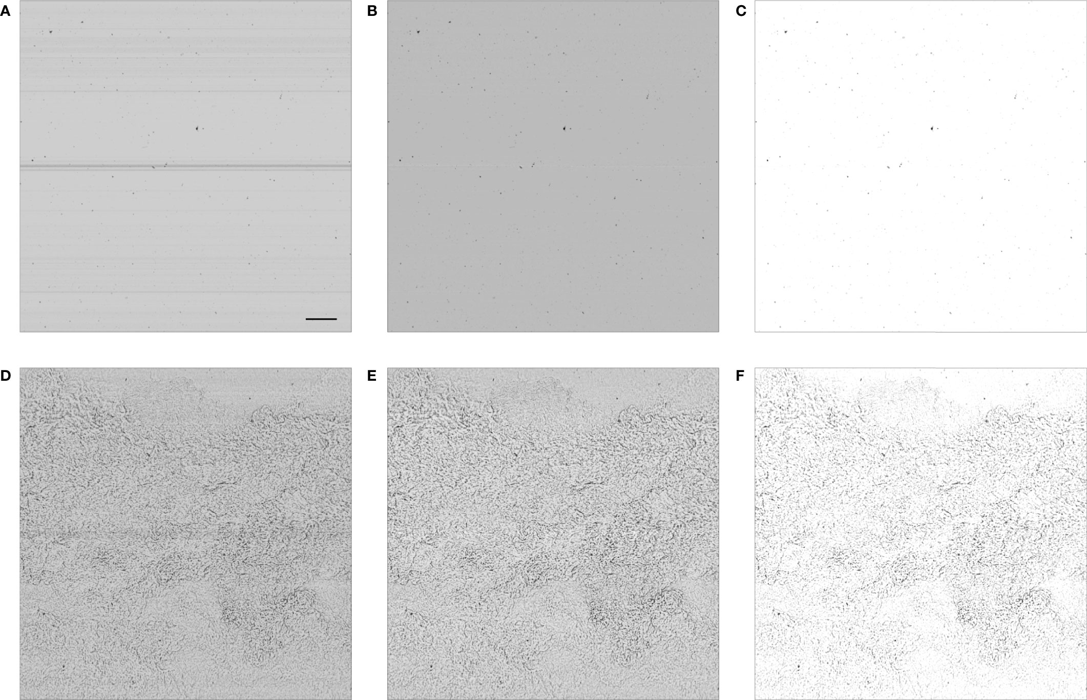
Figure 1 ISIIS frames in clean waters (A–C) and across a density change (D–F). The signature of this density change is similar to what a shadowgraph would image in air, above a burning candle. The panels are: (A, D) raw output; (B, E) after flat-fielding; (C, F) after contrasting. The camera scans vertically and the image is acquired from the right edge, as ISIIS moves through the water. In panel (A), the scale bar represents 1 cm and is applicable to other panels.

The very characteristics that give the ISIIS its qualities as a plankton imager (large sampling volume, high speed, ability to detect transparent objects) also mean that it creates a huge amount of images, the background of which is often non-uniform. This makes segmentation of planktonic objects from raw images far from trivial. To perform this segmentation, the processing pipeline was initially based on anomalies from a gaussian mixture model of the background gray levels without flat-fielding (Tsechpenakis et al., 2007) and later on k-harmonic means clustering on flat-fielded images (Iyer, 2012). This latter method was used in several studies (Luo et al., 2018; Greer et al., 2018; Schmid et al., 2020) and the full pipeline was open sourced in order to make plankton imaging more accessible and lower entry barriers (Schmid et al., 2021). Other studies relied on flat-fielding followed by segmentation above a fixed gray level (Faillettaz et al., 2016; Greer et al., 2020a; Greer et al., 2020b). However, most of these studies focused on the larger end of size range targeted by the ISIIS, by considering only objects above a given size threshold (Table 1), often because those were desirable targets, not noise. Similarly, for their canny edge detector applied to ZooGlider images, Ohman et al. (2019) considered objects larger than 100 pixels (Equivalent Spherical Diameter, or ESD of 0.45 mm). However, the algorithm failed when too many particles were present and had to fall back to a less sensitive (i.e. higher) gray threshold. As shown above, both planktonic organisms and particles are much more abundant towards the smaller end of the spectrum, meaning that such methods had to ignore a non-negligible part of planktonic organisms and marine snow in order to discard the background noise.

TABLE 1

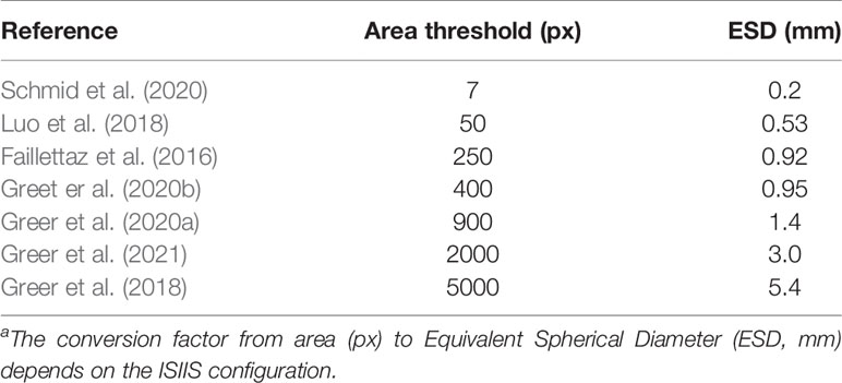
Table 1 Threshold in object area (number of pixels considered as part of the object) in studies exploiting ISIIS data.

1.3. Marine Snow and Imaging Artifacts Dominate In Situ Images and Complicate Plankton Detection

Marine snow particles are much more abundant than plankton in the ocean (Lombard et al., 2019), which means that the vast majority (often > 85%) of images captured by in situ plankton imaging instruments are actually of various marine snow items (fecal pellets, large aggregates, small organism pieces, etc.; (Stemmann et al., 2000; Picheral et al., 2010; Stemmann and Boss, 2012)). Therefore, for plankton ecology studies, the bottleneck has often become the processing and filtering of collected images (Irisson et al., 2022). To reduce the proportion of detrital particles and focus on photosynthetic plankton, the IFCB and the FlowCam can use fluorescence image triggering, hence imaging only items that contain chlorophyll (Sieracki et al., 1998; Sosik and Olson, 2007). This is not possible over the large volumes and for the non-photosynthetic organisms that ISIIS or other zooplankton imagers target. Furthermore, density anomalies lead to the characteristically noisy shadowgrams presented above (Figures 1D–F), from which numerous artifactual “particles” are detected by the usual image processing pipelines. Those artifacts or noise, together with marine snow, can constitute 99% of the objects detected. Such an extreme class imbalance makes the automatic classification of these objects through machine learning a very arduous task (Lee et al., 2016).

Even for a trained human operator, the differentiation of some planktonic classes from the proteiform marine snow aggregates and noise, as well as distinction between marine snow and noise themselves, can be very challenging. Towards the smaller end of the size spectrum it becomes virtually impossible. Indeed, once these small objects are segmented out, the low pixel count combined with the lack of information regarding their context in the image makes their identification very difficult, for humans and computers alike (Parikh et al., 2012). Hence, one solution could be to focus solely on planktonic organisms from the segmentation step already and try to avoid segmenting non-planktonic objects, thanks to their broader context in the image, still accessible at this step. This should result in a much more manageable amount of data to classify and a lesser class imbalance. This approach requires the development of specific and “intelligent” segmentation methods that target specific objects only. The purpose of this work was (i) to develop such “intelligent” segmentation approaches and (ii) to compare them with classic methods to test whether they significantly improve the data processing pipeline. With this in mind, we benchmarked three segmentation methods against a ground-truth human segmentation using a dataset collected by the ISIIS in the North-Western Mediterranean Sea.

2 Materials and Methods

2.1. Image Segmentation Methods

2.1.1. Threshold-Based Segmentation

The simplest segmentation method is to threshold pixels below a given gray level: adjoining pixels darker than the threshold are considered as segments. This threshold can be a value fixed a priori or dynamically computed from the properties of each image. For example, the classic method of Otsu (1979) is to examine the histogram of intensity levels and define the threshold so that it separates pixels into two relatively homogeneous intensity classes. Here either a fixed threshold was set or the threshold was defined based on a quantile of the histogram of gray levels. This quantile-based approach resulted in a darker segmentation threshold on noisy images, such as those captured around the strong density gradient induced by the thermocline (Figures 1D–F), which were richer in dark pixels. It was well adapted to limit the number of artifact segments generated from these images. Moreover, the first quartile is barely affected by the presence of relatively large dark objects such as jellyfish tentacles, making the segmentation threshold robust to these natural occurrences. After thresholding, segments defined by connected components were dilated by 3 pixels and eroded by 2 pixels to fill potential holes in transparent organisms and reconnect thin appendages to the organisms bodies. Finally, only segments larger than 50 pixels (400 µm in ESD) were retained, because it was the minimum size at which taxonomists could recognise organisms.

2.1.2. Threshold-MSER (T-MSER) Segmentation

This approach uses a signal-to-noise ratio (SNR) cutoff, calculated on images after flat-fielding, to determine whether the frame should be segmented using a Maximally Stable Extremal Region approach (MSER, Matas et al. (2004)), or if areas of high noise should first be filtered out using a naive thresholding approach before applying MSER. MSER was successfully applied to the segmentation of ZOOVIS imagery (Bi et al., 2015; Cheng et al., 2019). SNR can be used to determine the relative noise level in an image and was computed as

$\begin{array}{ll}\text{SNR}=20\times \text{log }\left(\frac{S}{N}\right)& (1)\end{array}$

where S is the signal, defined as the mean of the input data, and N is the noise, computed as the standard deviation around that mean. Here, flat-fielded frames with low SNR (i.e. high noise) were binarized using a fixed thresholding in order to extract continuous regions of interest with darker pixel values. The regions identified in this way were then extracted using a mask and subsequently re-segmented using the MSER approach. MSER detects stable connected regions in images, which are areas that stay nearly unchanged over a wide range of grayscale thresholds. MSER can be tuned to allow for varying degrees of stable region area and the range of pixel gray values tested in the dynamic thresholding. High SNR frames are directly segmented using the MSER approach (Figure 2 skip from step B to step D). Going from a pure MSER approach to the threshold+MSER (T-MSER) on low SNR (< 50) frames increased the recall on the test data from 65% to 85%, while also substantially increasing precision. This SNR and MSER method is written in C++17. The OpenCV and OpenMP Python packages were used for general computer vision and parallel processing for high processing efficiency, respectively.

FIGURE 2

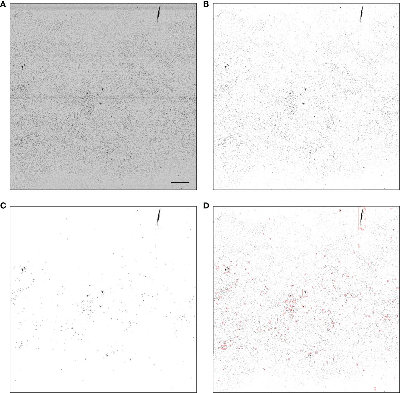
Figure 2 Example MSER segmentation of a noisy raw frame (with low SNR). (A) Raw output; (B) after flat-fielding; (C) regions of interest created through naive thresholding; (D) regions of interest and their bounding boxes created by applying MSER to (C). In a low SNR frame such as the one above the processing steps are (A–D), while in a high SNR frame the processing steps are (A, B, D). In panel (A), the scale bar represents 1 cm and is applicable to other panels.

2.1.3. Threshold-CNN (T-CNN) Segmentation

Another solution is to use Convolutional Neural Networks to either detect (i.e. define bounding boxes around) or segment (i.e. define a pixel mask of) objects of interest. Such approaches open the possibility to focus the detection on some types of objects (here, plankton) and ignore others (here, marine snow and artifacts); this is also called content-aware object detection or segmentation. However, CNNs tend to underperform at detecting objects across a large size range, especially for objects starting from a few dozen pixels (Cai et al., 2016). They work best when the target objects are of the same size as the receptive field of the model (Eggert et al., 2016). Thus, the development of detectors implementing receptive fields of various sizes constituted a major improvement, as they allowed detecting objects across a larger size range (Cai et al., 2016). In particular, we chose the Detectron2 library (Wu et al., 2019) developed by Facebook AI Research, which provides state-of-the-art object detection and segmentation algorithms, as well as pre-trained models for such tasks. Detectron2 includes a feature pyramid network (Lin et al., 2017) backbone that extracts feature maps across multiple scales to enable the detection of objects of various sizes, which was critical in our application to plankton images. Yet, this was not enough to cover the very large size range of organisms imaged by the ISIIS (from 50 to hundreds of thousands of pixels in area).

As explained above, marine snow particles and density-induced imaging artifacts are especially dominant compared to plankton in the smaller size classes. Therefore, our CNN pipeline was set up to segment the smaller objects, from 50 to 400 pixels in area, where the ability to specifically segment plankton makes the most difference. Above 400 pixels, the quantile-based threshold approach, with dilation and erosion, was used because it was simple and did not generate too many non-plankton segments.

In Detectron2, we used Mask R-CNN (He et al., 2017), which allows simultaneous bounding box detection and instance segmentation. The model was initialized with weights trained on the COCO reference dataset¹ but, for it to detect planktonic organisms on ISIIS images, it has to be fine-tuned on a dataset of ground truth bounding boxes and masks of such organisms. This dataset was generated by manually delineating all recognizable planktonic organisms in a set of ISIIS images, using a digital pen on a tablet computer. This produced 23,197 ground truth masks, from which bounding boxes were computed. Among those, 10,878 object were in the 50-400 pixels area range and usable. A 524×524 pixels crop was generated around every ground truth object (pushing the crop back inside the image when it crossed the edges). The choice of this particular size is a tradeoff between the maximum size of planktonic organisms that can be detected and the memory available on the graphics card. Moreover, it is in the line with common input sizes for segmentation models and was convenient to generate a tiling on ISIIS images. Several objects could be present in a crop. The crops were then split into 70% for training, 15% for validation, and 15% for testing. This split was stratified by the average gray level of the crop to ensure that both noisy (darker) and clean (lighter) images were present in each split, so that the model was presented with all kinds of images during training. Indeed, a model trained on clean images only would have performed poorly on noisy ones.

Detectron2 can perform multiclass object detection or segmentation, meaning that objects are both detected/segmented and classified in a single step. However, it requires sufficient examples in each class for training. This condition could not be satisfied here, given how time-consuming it was to obtain pixel-level masks for every object and because plankton samples are usually dominated by a few abundant taxa while most others are very rare (Ser-Giacomi et al., 2018). Since the focus of this study is on segmentation, we decided to perform one-class object detection/segmentation, thus training the model to recognize planktonic organisms of any taxon. This implies that classification needs to be done after segmentation. Once an object is detected, this sequential, rather than concurrent, approach does not affect the result of the classification, since the same information is available to the subsequent classifier as to the concurrent one. Furthermore, focusing on segmentation only is also more comparable with the two other methods described above.

The model was trained for 30,000 iterations, and evaluation was run on the validation set every 1,000 iterations to ensure that the validation loss reached a plateau. The learning rate was set to 0.0005 initially and decreased 10 fold after 10,000 and 20,000 iterations. To increase the generality of the detector, data augmentation was used in the form of random resizing of the 524 pixels crops (to 640, 672, 704, 736, 768 or 800 pixels) and random horizontal flipping. The test set was used to assess theoretical performance after training and guide the choice of model settings; the actual performance was assessed on a separate, real-world dataset (presented below).

To apply the trained model to new images, a tiling of 524×524 pixels crops (the size used during model training) was generated over each input image, resulting in an overlap of 143 pixels vertically and 135 pixels horizontally. The overlap ensured that detectable objects spread over two crops were not missed. Crops were upscaled to 900×900 pixels to improve detection of small objects (Eggert et al., 2016). For each crop, the model predicted the bounding boxes of objects and their masks. We only considered the boxes, resolved overlaps in detections caused by overlapping crops, and submitted each box to exactly the same quantile-based thresholding as what was used above 400 pixels. This was preferred over using Detectron’s mask proposals because their outline was not as detailed or replicable as the threshold-based ones. Furthermore, it also ensured that morphometric measurements performed on the masks (area in particular) were exactly comparable between the objects that went through the CNN and those above 400 pixels that were defined by simple thresholding. For each bounding box proposal, the model computes a confidence score. We retained all boxes with a score over 0.1, which is a quite low confidence threshold designed to increase the chance of detecting all objects of interest (i.e. favor recall) at the cost of some false positive detections (i.e. lower precision). Those false positives (i.e. segmented objects that are not plankton) will have the opportunity to be eliminated later, when segments are classified taxonomically.

The CNN was coded in Python with PyTorch, the original implementation library for Detectron2. Training was conducted on an Nvidia Quadro RTX 8000 GPU and the code is available at https://github.com/ThelmaPana/Detectron2_plankton_training. The combined CNN and threshold segmentation pipeline is implemented in https://github.com/jiho/apeep and this was run in several Linux-based environments, using various Nvidia GPUs.

2.2. Application to ISIIS Data from VISUFRONT Campaign

We evaluated these segmentation methods on ISIIS data from the VISUFRONT campaign, which sampled the Ligurian current front (North Western Mediterranean Sea), in the 0-100 m depth range, during summer 2013. Towed at a speed of 2 m s^-1 (4kts) and set for a 28 kHz scanning rate, the ISIIS sampled 108 L per second. The 2048 pixels high continuous image strip created by the line scan camera moving in the water was cut in 2048×2048 pixels frames for storage. The ISIIS captured marked volutes caused by water density variations (Figures 1D–F), mostly driven by temperature changes around the thermocline, previously described by Faillettaz et al. (2016).

The continuous image strip was reassembled from the stored 2048×2048 pixels frames. Each line of pixels was flat-fielded by subtracting the row-wise average over a 8000 pixels moving window, hence removing streaks (Figures 1A, B, D, E). The cleaned image was cut into 10,240 pixels long images (5 frames, instead of 1) to reduce the probability of cutting objects across images while keeping the memory footprint of each image manageable. Finally, the image was contrasted by stretching the intensity range between percentiles 0 and 40 (Figures 1B, C, E, F). These values were chosen by iteration, through discussions with the taxonomist in charge of delineating planktonic organisms from raw images, as to achieve the highest distinguishability for those.

A ground truth dataset was generated by manually delineating all planktonic organisms (using a digital pen and tablet) in 106 10,240×2048 pixels images, regularly spread across a full transect, hence representative of different environments. This resulted in 3,356 objects that were later taxonomically sorted into 24 taxa (Figure 3), in the Ecotaxa web application (Picheral et al., 2017). This dataset was completely independent from the one that was used to train, validate and test the Detectron2 model. Some images were checked by two independent operators to check their consistency; when this was done, no differences were found.

FIGURE 3

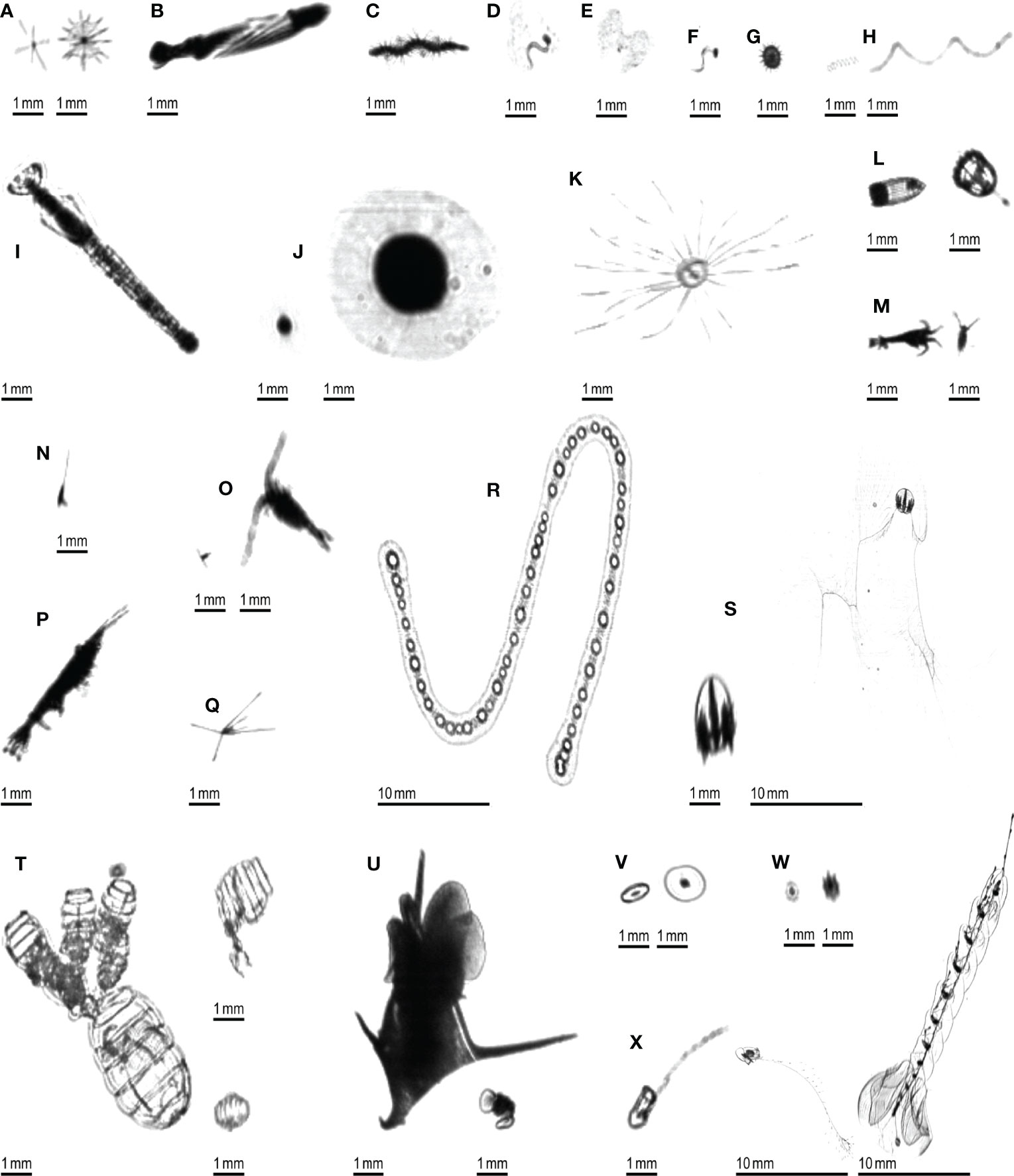
Figure 3 Examples of planktonic organisms imaged by the ISIIS. (A) Acantharea; (B) Actinopterygii; (C) Annelida; (D) Appendicularia; (E) Appendicularia (house only); (F) Appendicularia (body only); (G) Aulacanthidae; (H) Bacillariophyceae; (I) Chaetognatha; (J) solitary Collodaria; (K) Hydrozoa; (L) Cnidaria (other than Hydrozoa); (M) Crustacea (other than Harpacticoida, Copepoda and Eumalacostraca); (N) Harpacticoida; (O) Copepoda (other than Harpacticoida); (P) Eumalacostraca; (Q) Echinodermata (pluteus larva); (R) colonial Collodaria; (S) Ctenophora; (T) Doliolida; (U) Mollusca; (V) Pyrocystis; (W) Rhizaria (other than Acantharea; Aulacanthidae and Collodaria); (X) Siphonophorae.

Segments from each of the three automated methods were matched with ground truth segments of the same image. A bounding box intersection over union (IoU) score higher than 10% was considered as a match between segments. This threshold was set after manually inspecting a set of potential matches with various IoU values and was found to be the best value to discriminate between true and false matches. In case a ground truth segment matched multiple automatic segments, only one match was retained, to avoid inflating artificially the number of matches from the automated pipelines. In case an automatic segment matched multiple ground truth segments, the match was not counted either because it corresponded to a large segment that encompassed several organisms likely belonging to different taxa, which would make it unexploitable ecologically. Both choices made the match metrics conservative.

From these matches, global precision and recall were computed to summarize performance. Precision was computed as the proportion of automatic segments that matched ground truth segments. A 100% precision means that the algorithm only extracted ground truth segments. Recall was computed as the proportion of ground truth segments detected by the automated segmentation algorithm. A 100% recall means the algorithm did segment every manually delineated organism. Precision and recall scores were also computed per size class, where size was defined as the length of the diagonal of the bounding box; size classes were defined as intervals of 10 pixels, from 10 to 100 pixels, plus a class > 100 pixels. These size classes do not aim at reflecting any ecological groups but were designed to split segments into roughly balanced classes. Recall was also computed for each taxonomic group defined in the ground truth segments. Precision does not make sense for taxonomic groups since it would only reflect the performance of the classification, not of the segmentation. The particle matching and metric computation code is available at https://github.com/ThelmaPana/segmentation_benchmark.

3 Results

3.1. Number and Size Distribution of Segments

On the 106 images of the segmentation benchmark dataset, 3,356 organisms were manually segmented, whereas the automated pipelines generated many more segments, especially the threshold-based one (Table 2).

TABLE 2

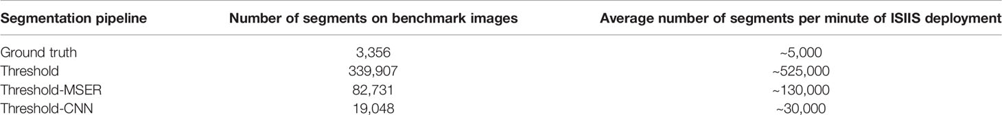
Table 2 Number of segments generated by each pipeline on the 106 benchmark images and estimation of the amount of segments they would produce on one minute of ISIIS data.

The normalized abundance size spectra (NASS) (Figure 4) display the expected linear decrease of abundance with size in log-log scale. For the ground truth segments, the curve dips below this linear relationship for objects of 25 pixels in diagonal and smaller (dotted vertical line on Figure 4). Since this dataset specifically targeted recognisable planktonic organisms, this dip highlights that not all organisms below this size could be detected by a human taxonomist upon detailed examination of the images (Lombard et al., 2019). The discontinuity is towards smaller diagonal sizes in the automated pipelines, but likely because many of the small segments are of non-plankton objects.

FIGURE 4

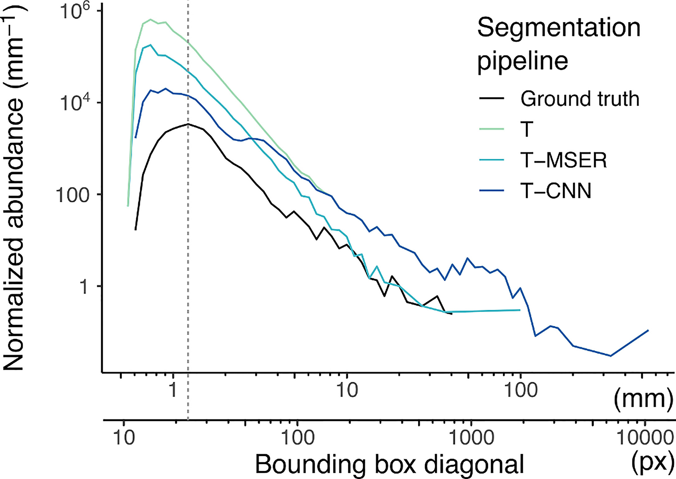
Figure 4 Normalized abundance size spectra (NASS) of all segments generated by the benchmarked pipelines and ground truth segmentation. To compute the NASS, segments were grouped into size classes on a log2 scale, each class size being two times wider than the previous one. Normalized abundance was computed by dividing the number of segments in each class by the size class width, resulting in an adimensional quantity (number of segments) divided by a length (mm here). The double x-axis is the length of the diagonal bounding box displayed both in pixels and after conversion in mm. The dotted vertical line highlights the slope discontinuity in the size spectrum of ground truth segments. Note that both axes use log10 scaling. T, threshold-based; T-MSER, threshold-MSER; T-CNN, threshold-CNN.

All automated pipelines have NASS curves above the ground truth, which highlights the fact that they segmented non-plankton objects. This was true over the entire size range but was particularly pronounced for the smaller size classes. Above 10 mm/200 pixels in diagonal, the T-MSER pipeline produced a number of segments comparable to the ground truth, which is satisfying, although it does not guarantee that those are of the same objects (it might have missed some plankton and segmented marine snow/artifacts in the same size range; see precision and recall performances for the largest size class in Figure 5 below). From the maximal size down to ~70 pixels in diagonal, the T and T-CNN pipelines produced the same segments. This coincides with the critical size of 400 pixels in area at which the segmentation method switched from threshold-based to content-aware. Indeed, the conversion from area to bounding box diagonal is not linear because it depends on the shape of the objects. For an object of 400 pixels in area, the bounding box diagonal is between 30 and 70 pixels. This shows that the T-CNN pipeline was effective in reducing the number of segments compared to naive thresholding, because the NASS diverges below that size.

FIGURE 5

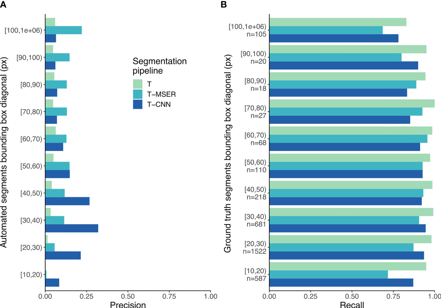
Figure 5 Precision (A) and recall (B) scores per size class. In (B), n indicates the number of segments per size class for the ground truth dataset. T, threshold-based; T-MSER, threshold-MSER; T-CNN, threshold-CNN.

A linear regression performed on the linear portion of the NASS (diagonal values between 30 and 500 pixels) followed by an analysis of covariance demonstrated significant difference in slopes between the segmentation methods: F(3,105) = 133.07; p < 0.001 (Table S1). Post hoc analysis showed a significant difference between all segmentation methods (p < 0.001 for all pairs) (Table S2).

3.2. Global Performance Statistics

Overall, the three pipelines demonstrate good recall: when looking at the total number of segments, they all captured over 85% of the ground truth organisms. The T-CNN pipeline largely outperformed both the threshold-based and T-MSER pipelines in terms of precision (Table 3). In other words, although it segmented almost all planktonic objects, the threshold-based pipeline generated mostly non-plankton segments (~99%), composed of both marine snow and density volutes artifacts. The T-CNN pipeline also produced non-planktonic segments but they “only” represented 84% of segments, while still segmenting a good proportion of planktonic objects. The T-MSER performed somewhere in between those two extremes.

TABLE 3

Table 3 Precision and recall values of the automated pipelines evaluated against the 3,356 ground truth organisms.

3.3. Performances Per Size Class

Because the behavior of the pipelines seems to vary with size (Figure 4), it seems relevant to break down the matching statistics per size class. With the threshold-based pipeline, precision decreased with size: smaller segments included a lower proportion of planktonic organisms than larger ones (Figure 5A). The T-CNN pipeline had better precision than the others for small segments while T-MSER had a better precision for larger segments. In terms of recall, the threshold-based pipeline always performed better than the others, regardless of size class (Figure 5B). The T-MSER pipeline performed as well as the T-CNN pipeline on middle size classes, but achieved a lower recall for both very small and very large segments.

3.4. Performances Per Taxonomic Group

In the ground truth dataset, half of the 24 detected taxa were represented by fewer than 18 individuals (median is 18.5), hence inducing little resolution and large variance in the performance statistics of segmentation pipelines. Among the other half of the taxa, the recall of the T-CNN pipeline was lower than that of the threshold pipeline by more than 10% for only two taxa (Bacillaryophycea and Doliolida) and for only four in the case of the T-MSER pipeline (Bacillariophyceae, Ctenophora, Acantharea, and other Rhizaria; Figure 6). The lowest recall values were reached for Bacillariophyceae and Ctenophora, for all pipelines. In concordance with the consistent recall performance across size classes, taxa-wise recall performance of the T-CNN pipeline do not seem linked to organism size: small organisms (e.g. Acantharea, Pyrocystis) were accurately detected.

FIGURE 6

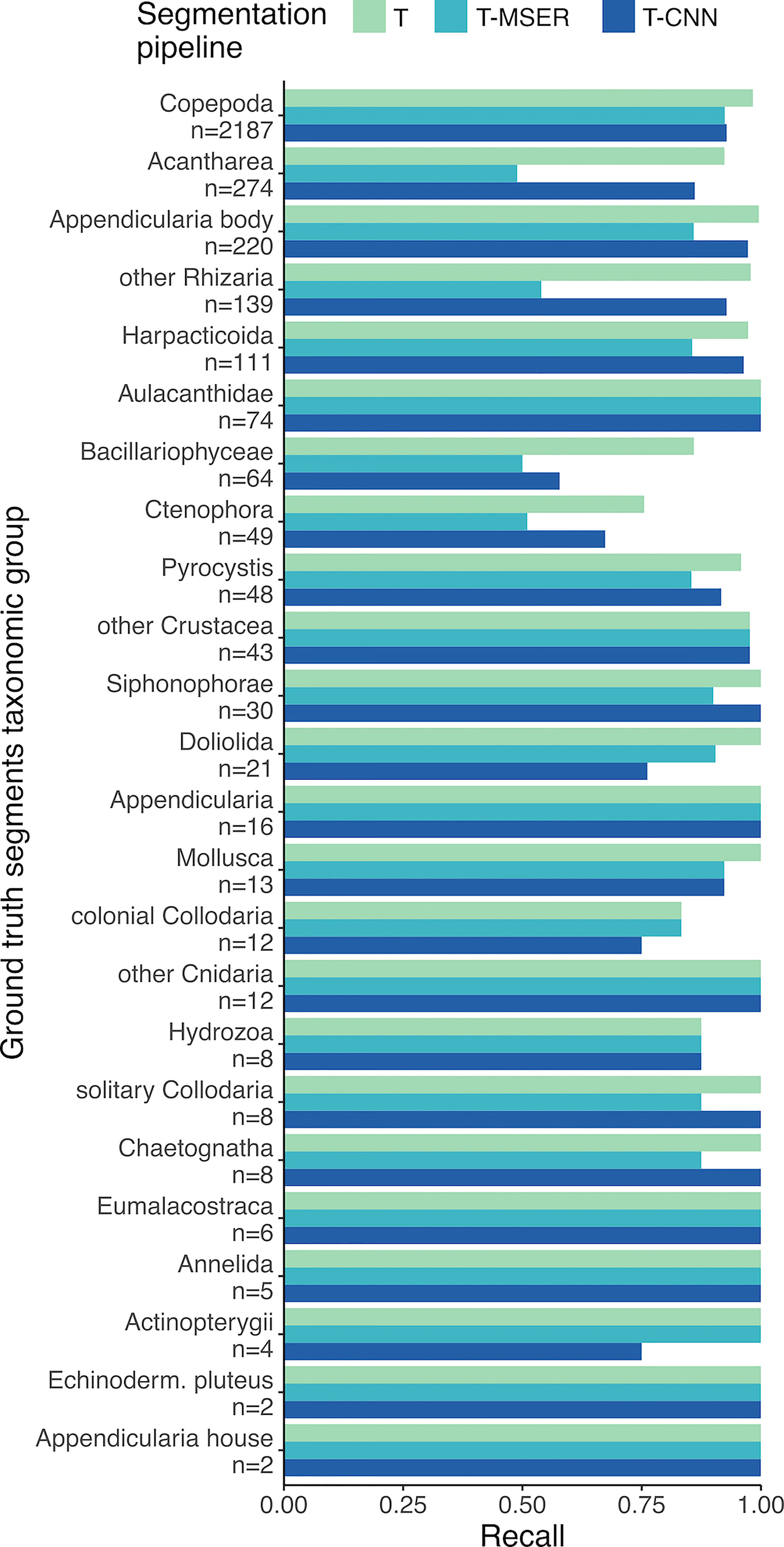
Figure 6 Recall scores per taxon. n is the number of individuals from each taxon in the 106 benchmark images and taxa are sorted in decreasing order of abundance. T, threshold-based; T-MSER, threshold-MSER; T-CNN, threshold-CNN.

4 Discussion

4.1. Summary of Results

The threshold-based pipeline performed an exhaustive segmentation: planktonic organisms were almost all properly detected, yet they were drowned in the overwhelming majority of non-planktonic objects (Table 2). The T-CNN pipeline reduced this problem, significantly increasing precision (Table 3 and Figure 5A) while still achieving a very good detection of plankton across the entire size range targeted by ISIIS. The T-MSER pipeline also reduced the segmentation of non-planktonic objects, especially at the top-end of the size range, but detected fewer planktonic organisms than the other pipelines (Figure 5B). Despite the large decrease in number of segmented objects, for most taxa, the MSER or CNN pipelines reduced recall by less than 10% (Figure 6). One explanation for these differences is that naive thresholding captured a lot of noise (i.e. density volutes) and, additionally, broke it into many small segments. The use of either MSER or a CNN allowed ignoring these noise segments and/or not breaking them apart, hence producing much fewer non-planktonic segments. The decrease in abundance below the expected slope at the smaller end of the size spectrum of ground truth segments (Figure 4) suggests that identification of planktonic organisms becomes non-exhaustive below 25 pixels in bounding box diagonal. Below this size, which amounts to 600 µm in ESD on average, some organisms can still be detected. This means that relative concentrations between locations/times can likely be exploited within a taxon but that further filtering and corrections are needed to reach absolute concentrations.

The statistical difference between NASS slopes (Figure 4) indicates that they segment different kinds and amounts of non-planktonic objects, compared to the all-plankton ground truth. This implies that the output of different segmentation approaches should not be directly compared in terms of size distribution. Segmentation methods were already shown to have an impact on the definition of particle size and shape, which propagates to subsequent analyses such as particle flux estimates (Giering et al., 2020). This slope discrepancy as well as the vastly larger intercept of the NASS of automated pipelines compared to the ground truth means that the computation of an appropriate plankton size spectrum requires a classification step that would exclude non-planktonic objects.

4.2. Targeted Organisms

Some taxa were systematically less often detected than others. Some of the not detected Bacillariophyceae were large, blurry, and too translucent (Figure 3H) to be caught by the threshold-based branch of the T-CNN pipeline or by the T-MSER method. The other, smaller, ones that were missed by the content-aware branch of T-CNN were not detected because they were quite different from the ones used during training (blurrier). Integrating more representative examples of Bacillariophyceae for CNN training could have improved performance on this taxon. Similarly, doliolids (Figure 3T), that were often large, should have been segmented by the threshold-based branch of T-CNN as well as by T-MSER. The ones missed, mostly by T-CNN, were also blurry and too translucent for intensity-based thresholding with a single threshold. Ctenophores (likely of the Mertensiidae family, Figure 3S) displayed thin, translucent tentacles that were often missed by threshold-based methods. Therefore, only the body was segmented, which resulted in a bounding box IoU value < 0.1, too low to be considered a match with the ground truth segment that included the tentacles. Still, a later CNN classifier should be able to correctly identify even such portions of organisms, as CNNs were shown to mostly rely on local shape and texture features instead of on the global shape (Baker et al., 2018; Baker et al., 2020). Finally, the T-MSER pipeline resulted in a lower recall for Acantharea and other Rhizaria (Figures 3A, W). This seems to stem from a too aggressive thresholding step in low SNR high noise frames, the pre-processing step before MSER is applied. Further fine-tuning would likely allow it to retain more or all Acantharea and other Rhizaria images.

In the present study, we aimed at performing an exhaustive detection of every planktonic organism across the size range targeted by the ISIIS. However, in general, the segmentation algorithm should be chosen according to the target organisms. For example, to focus on organisms towards the larger end of the ISIIS size range (e.g. > 10 mm), where particles — mostly marine snow aggregates — are much less abundant, a simple gray-level threshold seems sufficient.

4.3. Processing Time and Cost

The quantile-based thresholding pipeline ran on a single CPU core at a rate of 30 minutes of processing for 1 minute of ISIIS data (0.03x), on an Intel Xeon E5-2643 v3 (3.40 GHz). Its memory requirements were limited so it was easy to run simultaneous processing of multiple batches of data on a multi-core/multi-processor machine, but the treatment of ISIIS data as a continuous stream for flat-fielding prevented automatic multithreading. The T-CNN pipeline required a GPU with sufficient memory (48 GB, on aNvidia Quadro RTX 8000 in our case) to efficiently train the CNN portion and to fit ISIIS images in at evaluation time. It processed data at the same rate as the threshold-based pipeline (30 min processing for 1 min of data, or 0.03x). The T-MSER pipeline was optimized for speed and utilized the 8 cores of an AMD Ryzen 3700, processing one minute of ISIIS data in 50 seconds (1.2x), or 6 min 40 s of processing for 1 min of ISIIS data (0.15x) when considering running on one core.

The MSER implementation followed Matas et al. (2004) closely. The optimization of the T-MSER approach stems from adding the SNR switch, which leads to the pre-processing of high-noise images with naive thresholding, while going straight to the MSER-based detection in low noise images. Adding these changes increased segmentation recall from 65% to 85%. Further optimization included making the code multi-thread ready for deployment on High Performance Computing infrastructures. Using the specialized CPUs of these infrastructures, such as the AMD EPYC 7742 (64 cores, 128 threads) performance could improve well above 1.2x. At current data collection rates of 75-100 h of ISIIS data per scientific cruise, a real time or faster than real time segmentation approach constitutes a substantial benefit.

At first glance, the T-CNN pipeline seems expensive in terms of set up and architecture: it requires a GPU with sufficient memory to operate, implies the use of relatively new deep learning coding frameworks and the preparation of a training set with manual delineation of thousands of planktonic organisms. But these costs are offset by the time gained not processing a multitude of particles in each image, resulting in a processing rate comparable to that of the pure threshold-based pipeline, as stated above. Furthermore, the fact that T-CNN produced 20 times fewer segments will also considerably reduce the classification time (often CNN based too). Finally, since recall barely decreased, the objects ignored were mostly the dominant non-plankton objects, as per design; this will diminish the imbalance among classes that classifiers are sensitive too, further improving the classification step. Moreover, both the Detectron2 library and the baseline model on which the T-CNN pipeline relies are easily downloadable and well documented². With GPU resources becoming increasingly available for scientific research and the associated frameworks becoming easier to use, such tools are poised to become more powerful and accessible.

4.4. Detection of Small Objects by CNN Models

The detection of objects measuring just a few pixels is still a research problem in its own right in computer sciences (Eggert et al., 2017), coined very low resolution recognition problems (Wang et al., 2016). They are characterized by targets smaller than 16×16 pixels, which can be challenging even for the perceptual abilities of human experts. They target applications for company logo detection (Eggert et al., 2016; Eggert et al., 2017), face recognition from video surveillance, or text recognition (Wang et al., 2016). The receptive fields of common object detection architectures match the target object size and range from 50×50 to 450×450 pixels which is much larger than the small objects targeted in low resolution studies (Eggert et al., 2017). Here, the smallest organisms targeted had an area of 50 pixels, which corresponded to a bounding box diagonal of 12 pixels, or an 8x8 pixels square. Thus the exhaustive detection of plankton organisms in ISIIS images, including the smaller ones, clearly falls in the domain of very low resolution recognition. A common solution is image upscaling, as highlighted by Eggert et al. (2016), which we implemented in the present work. The 524×524 pixels crops were upscaled to 900×900 pixels before evaluation in the Detectron2 model. The 900 pixels size is a compromise between detection accuracy, usage of the GPU memory, and processing time. Other approaches for multi-scale object detection are described by (Cai et al., 2016) and include magnification of regions susceptible to contain small objects (Eggert et al., 2016) or the integration of contextual information outside of regions of interest (Bell et al., 2016).

No automated segmentation method is perfect; depending on their settings, they either avoid objects other than their targets but miss some objects of interest (high precision, low recall) or detect most objects of interest but also many others (high recall, low precision). If the segmentation or object detection task is followed by a classification step, which is always the case for plankton imaging, we advocate in favor of recall over precision during segmentation, provided that the amount of data remains manageable. Hence, a maximum number of planktonic objects have the opportunity to be classified. The precision can be improved after classification, by filtering out low confidence, usually error prone, predictions based on the score given by the classifier (Faillettaz et al., 2016; Luo et al., 2018).

To extract planktonic organisms of various taxa from ISIIS images, full instance segmentation would have been the most elegant approach, outputting classified mask instances in a single step (Dai et al., 2016). Several obstacles still lay ahead for this approach to be applicable. First, training an instance segmentation model to recognize each taxonomic group would require hundreds to thousands of ground truth (i.e. human-produced) masks of all taxa. Given the long tailed distribution of taxa concentrations in the planktonic world, with many rare taxa, in particular the largest ones, this would require a considerable amount of searching and labeling effort. Indeed, assembling enough examples to train classifications models is already challenging (Irisson et al., 2022) and manual delineation of each organism is much more time consuming than manual classification. A second obstacle is the size range of organisms imaged by ISIIS. Although Detectron2 does produce multi-scale feature maps through a Feature Pyramid Network in order to apply receptive fields of multiple size, the ratio between the largest and the smallest feature maps is only 16. Here, the ratio between the smallest and largest bounding box diagonals of manually segmented organisms is 65 and can reach > 180 in more exhaustive ISIIS datasets. To tackle this span, one could theoretically set up an ensemble of detectors, fed with crops of different sizes, each one targeting a restricted size range. Yet, this would be a particularly computationally demanding and complex set up, for a gain yet to be determined since, for larger sizes, the proportion of non-plankton objects, and therefore the advantage of a CNN-based segmentation, diminishes. Finally, masks generated by instance segmentation models currently lack both precision (their outline is smoothed, not matching the fine appendages of plankton) and reproducibility (because of the randomness included during training to avoid overfitting, two models trained on the same data will output different masks). These drawbacks are particularly critical for plankton application, where the size of the organisms, computed from their masks, is often of interest.

5 Conclusion and Perspectives

We developed combined segmentation pipelines able to detect planktonic organisms spanning a broad size range. The fact that all methods comprised a deterministic, threshold-based segmentation ensured that particle shapes and measurement were consistent over the whole size range. Still, the segmentation method affected the shape of the size spectrum and additional processing steps (including classification) are needed to extract the correct size structure of living organisms. The MSER method limited over-segmentation of background noise objects and extracted more consistent segments, at a very high processing rate. This speed opens the possibility for near-real time processing, which is particularly relevant for adaptive sampling during a cruise or an early warning system in a time series context. Although at the lower limit of the detection capabilities of CNNs, our content-aware approach was able to detect planktonic organisms among an overwhelming number of marine snow and noise images, exhibiting the best recall of the three methods. Therefore, the ideal segmentation approach depends on the study objectives and operational constraints.

These approaches seem relevant for imaging studies focused on living planktonic organisms, since they reduce the number of objects from non-plankton classes that are extracted. In turn, this dampens the imbalance towards these classes, laying the foundations for easier, faster, and more accurate subsequent object classification by (i) reducing the amount of work needed to generate a training set with similar class distribution, which is essential to avoid the caveat of dataset shift (Moreno-Torres et al., 2012); (ii) decreasing the computation time because there are fewer objects; and (iii) limiting the contamination of the rare planktonic classes by the dominant, non-plankton, ones.

Although CNN-based object detection may seem overwhelming at first, both in terms of set up and processing time, it actually is fast enough and within the reach of marine ecologists, particularly now that artificial intelligence frameworks and GPU computing are being made more accessible. This work constitutes a step towards the “intelligent” segmentation of ecological images, even at low resolution, which could find even wider applications such as the automated separation of objects overlapping onto each other on an image for more accurate species counts, the detection and classification in a single step for more automated surveys, or the extraction of individual-level traits to track e.g., reproductive organs development, for a richer exploitation of ecological images (Orenstein et al., 2021). Such tasks are in no way limited to plankton images and are common in data collected by trawl cameras, benthic observations or surveying cameras, vessel monitoring cameras, etc.

In this era of data-driven oceanography, the volume of data collected is increasing sharply, thanks to technological advances such as high frequency imagery, autonomous instruments (e.g. floats, gliders), satellite-based methods as well as environmental -omics approaches permitted by high throughput sequencing. In this context of abundant data, the development of automated and efficient data processing techniques becomes a key element in drawing a holistic understanding of oceanic ecosystems; it is needed to provide an extensive description of biodiversity, including species distributions as well as estimates of biomass and abundance.

Data Availability Statement

The raw data supporting the conclusions of this article will be made available by the authors, without undue reservation.

Author Contributions

J-OI and TP conceptualized the study. LC-C and TP generated and taxonomically sorted ground truth plankton segments. BW and TP developed the CNN segmentation method. J-OI and TP developed the threshold-based and the T-CNN processing pipelines. MS, DD, ST, CS, and RC set up and ran the T-MSER method. TP prepared the original draft. All co-authors proof-read the manuscript prior to submission. All authors read and approved the final manuscript.

Funding

This study is part of project “World Wide Web of Plankton Image Curation”, funded by the Belmont Forum through the Agence Nationale de la Recherche ANR-18-BELM-0003-01 and the National Science Foundation (NSF) #ICER1927710. Funding also came from NSF #OCE2125407. The Extreme Science and Engineering Discovery Environment (XSEDE) provided computing resources to the US team through grant #TG-OCE170012. Data acquisition during the VISUFRONT cruise was funded by the Partner University Fund and supported by the French Oceanographic Fleet through ship time. TP’s doctoral fellowship was granted by the French Ministry of Higher Education, Research and Innovation (#3500/2019).

Conflict of Interest

Author Ben Woodward was employed by company CVision AI.

The remaining authors declare that the research was conducted in the absence of any commercial or financial relationships that could be construed as a potential conflict of interest.

Publisher’s Note

All claims expressed in this article are solely those of the authors and do not necessarily represent those of their affiliated organizations, or those of the publisher, the editors and the reviewers. Any product that may be evaluated in this article, or claim that may be made by its manufacturer, is not guaranteed or endorsed by the publisher.

Acknowledgments

The authors would like to thank the officers and crew of the R/V Tethys 2 who made the VISUFRONT campaign a success, as well as the additional scientists who took part in the cruise: R Faillettaz, C M Guigand, F Lombard, M Lilley, and J Luo.

Supplementary Material

The Supplementary Material for this article can be found online at: https://www.frontiersin.org/articles/10.3389/fmars.2022.870005/full#supplementary-material

Footnotes

1. ^ https://github.com/facebookresearch/detectron2/blob/main/configs/COCO-InstanceSegmentation/mask_rcnn_R_50_FPN_3x.yaml/

References

Alldredge A. L., Granata T. C., Gotschalk C. C., Dickey T. D. (1990). The Physical Strength of Marine Snow and Its Implications for Particle Disaggregation in the Ocean. Limnol. Oceanog. 35, 1415–1428. doi: 10.4319/lo.1990.35.7.1415

CrossRef Full Text | Google Scholar

Alldredge A. L., Silver M. W. (1988). Characteristics, Dynamics and Significance of Marine Snow. Prog. Oceanog. 20, 41–82. doi: 10.1016/0079-6611(88)90053-5

CrossRef Full Text | Google Scholar

Baker N., Lu H., Erlikhman G., Kellman P. J. (2018). Deep Convolutional Networks do Not Classify Based on Global Object Shape. PloS Comput. Biol. 14, e1006613. doi: 10.1371/journal.pcbi.1006613

PubMed Abstract | CrossRef Full Text | Google Scholar

Baker N., Lu H., Erlikhman G., Kellman P. J. (2020). Local Features and Global Shape Information in Object Classification by Deep Convolutional Neural Networks. Vision Res. 172, 46–61. doi: 10.1016/j.visres.2020.04.003

PubMed Abstract | CrossRef Full Text | Google Scholar

Bell S., Zitnick C. L., Bala K., Girshick R. (2016). “Inside-Outside Net: Detecting Objects in Context With Skip Pooling and Recurrent Neural Networks,” in Proceedings of the IEEE Conference on Computer Vision and Pattern Recognition (CVPR), 2874–2883.

Google Scholar

Benfield M., Grosjean P., Culverhouse P., Irigolen X., Sieracki M., Lopez-Urrutia A., et al. (2007). RAPID: Research on Automated Plankton Identification. Oceanography 20, 172–187. doi: 10.5670/oceanog.2007.63

CrossRef Full Text | Google Scholar

Biard T., Ohman M. D. (2020). Vertical Niche Definition of Test-Bearing Protists (Rhizaria) Into the Twilight Zone Revealed by in Situ Imaging. Limnol. Oceanog. 65, 2583–2602. doi: 10.1002/lno.11472

CrossRef Full Text | Google Scholar

Biard T., Stemmann L., Picheral M., Mayot N., Vandromme P., Hauss H., et al. (2016). In Situ Imaging Reveals the Biomass of Giant Protists in the Global Ocean. Nature 532, 504–507. doi: 10.1038/nature17652

PubMed Abstract | CrossRef Full Text | Google Scholar

Bi H., Guo Z., Benfield M. C., Fan C., Ford M., Shahrestani S., et al. (2015). ). A Semi-Automated Image Analysis Procedure for In Situ Plankton Imaging Systems. PloS One 10, e0127121. doi: 10.1371/journal.pone.0127121

PubMed Abstract | CrossRef Full Text | Google Scholar

Brandão M. C., Benedetti F., Martini S., Soviadan Y. D., Irisson J.-O., Romagnan J.-B., et al. (2021). Macroscale Patterns of Oceanic Zooplankton Composition and Size Structure. Sci. Rep. 11, 15714. doi: 10.1038/s41598-021-94615-5

PubMed Abstract | CrossRef Full Text | Google Scholar

Briseño-Avena C., Schmid M. S., Swieca K., Sponaugle S., Brodeur R. D., Cowen R. K. (2020). Three-Dimensional Cross-Shelf Zooplankton Distributions Off the Central Oregon Coast During Anomalous Oceanographic Conditions. Prog. Oceanog. 188, 102436. doi: 10.1016/j.pocean.2020.102436

CrossRef Full Text | Google Scholar

Cai Z., Fan Q., Feris R. S., Vasconcelos N. (2016). “A Unified Multi-Scale Deep Convolutional Neural Network for Fast Object Detectionv,” in European Conference on Computer Vision (ECCV), 1607.07155.

Google Scholar

Cheng K., Cheng X., Wang Y., Bi H., Benfield M. C. (2019). Enhanced Convolutional Neural Network for Plankton Identification and Enumeration. PloS One 14, e0219570. doi: 10.1371/journal.pone.0219570

PubMed Abstract | CrossRef Full Text | Google Scholar

Cowen R. K., Guigand C. M. (2008). In Situ Ichthyoplankton Imaging System (ISIIS): System Design and Preliminary Results. Limnol. Oceanog.: Methods 6, 126–132. doi: 10.4319/lom.2008.6.126

CrossRef Full Text | Google Scholar

Dai J., He K., Sun J. (2016). “Instance-Aware Semantic Segmentation via Multi-Task Network Cascades,” in Proceedings of the IEEE Conference on Computer Vision and Pattern Recognition (CVPR), 3150–3158.

Google Scholar

Dennett M. R., Caron D. A., Michaels A. F., Gallager S. M., Davis C. S. (2002). Video Plankton Recorder Reveals High Abundances of Colonial Radiolaria in Surface Waters of the Central North Pacific. J. Plank. Res. 24, 797–805. doi: 10.1093/plankt/24.8.797

CrossRef Full Text | Google Scholar

de Vargas C., Audic S., Henry N., Decelle J., Mahé F., Logares R., et al. (2015). Eukaryotic Plankton Diversity in the Sunlit Ocean. Science 348, 1261605. doi: 10.1126/SCIENCE.1261605

PubMed Abstract | CrossRef Full Text | Google Scholar

Eggert C., Brehm S., Winschel A., Zecha D., Lienhart R. (2017). “A Closer Look: Small Object Detection in Faster R-CNN,” in Proceedings of the IEEE International Conference on Multimedia and Expo (ICME), 421–426. doi: 10.1109/ICME.2017.8019550

CrossRef Full Text | Google Scholar

Eggert C., Winschel A., Zecha D., Lienhart R. (2016). “Saliency-Guided Selective Magnification for Company Logo Detection,” in 23rd International Conference on Pattern Recognition (ICPR), 651–656. doi: 10.1109/ICPR.2016.7899708

CrossRef Full Text | Google Scholar

Faillettaz R., Picheral M., Luo J. Y., Guigand C., Cowen R. K., Irisson J.-O. (2016). Imperfect Automatic Image Classification Successfully Describes Plankton Distribution Patterns. Methods Oceanog. 15–16, 60–77. doi: 10.1016/J.MIO.2016.04.003

CrossRef Full Text | Google Scholar

Falkowski P. (2012). Ocean Science: The Power of Plankton. Nature 483, S17–S20. doi: 10.1038/483S17a

PubMed Abstract | CrossRef Full Text | Google Scholar

Field C. B., Behrenfeld M. J., Randerson J. T., Falkowski P. (1998). Primary Production of the Biosphere: Integrating Terrestrial and Oceanic Components. Science 281, 237–240. doi: 10.1126/science.281.5374.237

PubMed Abstract | CrossRef Full Text | Google Scholar

Forest A., Stemmann L., Picheral M., Burdorf L., Robert D., Fortier L., et al. (2012). Size Distribution of Particles and Zooplankton Across the Shelf-Basin System in Southeast Beaufort Sea: Combined Results From an Underwater Vision Profiler and Vertical Net Tows. Biogeosciences 9, 1301–1320. doi: 10.5194/bg-9-1301-2012

CrossRef Full Text | Google Scholar

Frederiksen M., Edwards M., Richardson A. J., Halliday N. C., Wanless S. (2006). From Plankton to Top Predators: Bottom-Up Control of a Marine Food Web Across Four Trophic Levels. J. Anim. Ecol. 75, 1259–1268. doi: 10.1111/j.1365-2656.2006.01148.x

PubMed Abstract | CrossRef Full Text | Google Scholar

Giering S. L. C., Hosking B., Briggs N., Iversen M. H. (2020). The Interpretation of Particle Size, Shape, and Carbon Flux of Marine Particle Images Is Strongly Affected by the Choice of Particle Detection Algorithm. Front. Mar. Sci. 7. doi: 10.3389/fmars.2020.00564

CrossRef Full Text | Google Scholar

Greer A. T., Boyette A. D., Cruz V. J., Cambazoglu M. K., Dzwonkowski B., Chiaverano L. M., et al. (2020a). Contrasting Fine-Scale Distributional Patterns of Zooplankton Driven by the Formation of a Diatom-Dominated Thin Layer. Limnol. Oceanog. 65, 2236–2258. doi: 10.1002/lno.11450

CrossRef Full Text | Google Scholar

Greer A. T., Chiaverano L. M., Luo J. Y., Cowen R. K., Graham W. M. (2018). Ecology and Behaviour of Holoplanktonic Scyphomedusae and Their Interactions With Larval and Juvenile Fishes in the Northern Gulf of Mexico. ICES. J. Mar. Sci. 75, 751–763. doi: 10.1093/icesjms/fsx168

CrossRef Full Text | Google Scholar

Greer A. T., Chiaverano L. M., Treible L. M., Briseño-Avena C., Hernandez F. J. (2021). From Spatial Pattern to Ecological Process Through Imaging Zooplankton Interactions. ICES. J. Mar. Sci 78(8):2664–74. doi: 10.1093/icesjms/fsab149

CrossRef Full Text | Google Scholar

Greer A. T., Cowen R. K., Guigand C. M., Hare J. A. (2015). Fine-Scale Planktonic Habitat Partitioning at a Shelf-Slope Front Revealed by a High-Resolution Imaging System. J. Mar. Syst. 142, 111–125. doi: 10.1016/j.jmarsys.2014.10.008

CrossRef Full Text | Google Scholar

Greer A. T., Cowen R. K., Guigand C. M., Hare J. A., Tang D. (2014). The Role of Internal Waves in Larval Fish Interactions With Potential Predators and Prey. Prog. Oceanog. 127, 47–61. doi: 10.1016/j.pocean.2014.05.010

CrossRef Full Text | Google Scholar

Greer A. T., Cowen R. K., Guigand C. M., McManus M. A., Sevadjian J. C., Timmerman A. H. V. (2013). Relationships Between Phytoplankton Thin Layers and the Fine-Scale Vertical Distributions of Two Trophic Levels of Zooplankton. J. Plank. Res. 35, 939–956. doi: 10.1093/plankt/fbt056

CrossRef Full Text | Google Scholar

Greer A. T., Lehrter J. C., Binder B. M., Nayak A. R., Barua R., Rice A. E., et al. (2020b). High-Resolution Sampling of a Broad Marine Life Size Spectrum Reveals Differing Size- and Composition-Based Associations With Physical Oceanographic Structure. Front. Mar. Sci. 7 (8), 2664–2674. doi: 10.3389/fmars.2020.542701

CrossRef Full Text | Google Scholar

Guidi L., Jackson G. A., Stemmann L., Miquel J. C., Picheral M., Gorsky G. (2008). Relationship Between Particle Size Distribution and Flux in the Mesopelagic Zone. Deep. Sea. Res. Part I.: Oceanog. Res. Pap. 55, 1364–1374. doi: 10.1016/J.DSR.2008.05.014

CrossRef Full Text | Google Scholar

Guidi L., Legendre L., Reygondeau G., Uitz J., Stemmann L., Henson S. A. (2015). A New Look at Ocean Carbon Remineralization for Estimating Deepwater Sequestration. Global Biogeochem. Cycle. 29, 1044–1059. doi: 10.1002/2014GB005063

CrossRef Full Text | Google Scholar

He K., Gkioxari G., Dollar P., Girshick R., Mask R-CNN (2017). Proceedings of the IEEE International Conference on Computer Vision (ICCV). 2961–2969.

Google Scholar

Ibarbalz F. M., Henry N., Brandão M. C., Martini S., Busseni G., Byrne H., et al. (2019). Global Trends in Marine Plankton Diversity Across Kingdoms of Life. Cell 179, 1084–1097.e21. doi: 10.1016/j.cell.2019.10.008

PubMed Abstract | CrossRef Full Text | Google Scholar

Irisson J.-O., Ayata S.-D., Lindsay D. J., Karp-Boss L., Stemmann L. (2022). Machine Learning for the Study of Plankton and Marine Snow From Images. Ann. Rev. Mar. Sci. 14, 277–301. doi: 10.1146/annurev-marine-041921-013023

PubMed Abstract | CrossRef Full Text | Google Scholar

Iyer N. (2012). Machine Vision Assisted in Situ Ichthyoplankton Imaging System (Purdue University).

Google Scholar

Lee H., Park M., Kim J. (2016). “Plankton Classification on Imbalanced Large Scale Database via Convolutional Neural Networks With Transfer Learning,” in IEEE International Conference on Image Processing (ICIP), 3713–3717. doi: 10.1109/ICIP.2016.7533053

CrossRef Full Text | Google Scholar

Lévy M., Franks P. J. S., Smith K. S. (2018). The Role of Submesoscale Currents in Structuring Marine Ecosystems. Nat. Commun. 9, 4758. doi: 10.1038/s41467-018-07059-3

PubMed Abstract | CrossRef Full Text | Google Scholar

Lin T.-Y., Dollár P., Girshick R., He K., Hariharan B., Belongie S. (2017). “Feature Pyramid Networks for Object Detection,” in Proceedings of the IEEE Conference on Computer Vision and Pattern Recognition (CVPR), 1612.03144.

Google Scholar

Lombard F., Boss E., Waite A. M., Vogt M., Uitz J., Stemmann L., et al. (2019). Globally Consistent Quantitative Observations of Planktonic Ecosystems. Front. Mar. Sci. 6, 196. doi: 10.3389/fmars.2019.00196

CrossRef Full Text | Google Scholar

Longhurst A. R., Glen Harrison W. (1989). The Biological Pump: Profiles of Plankton Production and Consumption in the Upper Ocean. Prog. Oceanog. 22, 47–123. doi: 10.1016/0079-6611(89)90010-4

CrossRef Full Text | Google Scholar

Luo J. Y., Grassian B., Tang D., Irisson J.-O., Greer A. T., Guigand C. M., et al. (2014). Environmental Drivers of the Fine-Scale Distribution of a Gelatinous Zooplankton Community Across a Mesoscale Front. Mar. Ecol. Prog. Ser. 510, 129–149. doi: 10.3354/meps10908

CrossRef Full Text | Google Scholar

Luo J. Y., Irisson J.-O., Graham B., Guigand C., Sarafraz A., Mader C., et al. (2018). Automated Plankton Image Analysis Using Convolutional Neural Networks. Limnol. Oceanog.: Methods 16, 814–827. doi: 10.1002/lom3.10285

CrossRef Full Text | Google Scholar

Matas J., Chum O., Urban M., Pajdla T. (2004). Robust Wide-Baseline Stereo From Maximally Stable Extremal Regions. Imag. Vision Comput. 22, 761–767. doi: 10.1016/j.imavis.2004.02.006

CrossRef Full Text | Google Scholar

McClatchie S., Cowen R., Nieto K., Greer A., Luo J. Y., Guigand C., et al. (2012). Resolution of Fine Biological Structure Including Small Narcomedusae Across a Front in the Southern California Bight. J. Geophys. Res.: Ocean. 117, C04020. doi: 10.1029/2011JC007565

CrossRef Full Text | Google Scholar

Moreno-Torres J. G., Raeder T., Alaiz-Rodríguez R., Chawla N. V., Herrera F. (2012). A Unifying View on Dataset Shift in Classification. Pattern Recognit. 45, 521–530. doi: 10.1016/j.patcog.2011.06.019

CrossRef Full Text | Google Scholar

Ohman M. D., Davis R. E., Sherman J. T., Grindley K. R., Whitmore B. M., Nickels C. F., et al. (2019). Zooglider: An Autonomous Vehicle for Optical and Acoustic Sensing of Zooplankton. Limnol. Oceanog.: Methods 17, 69–86. doi: 10.1002/lom3.10301

CrossRef Full Text | Google Scholar

Olson R. J., Sosik H. M. (2007). A Submersible Imaging-in-Flow Instrument to Analyze Nano-and Microplankton: Imaging FlowCytobot. Limnol. Oceanog.: Methods 5, 195–203. doi: 10.4319/lom.2007.5.195

CrossRef Full Text | Google Scholar

Orenstein E. C., Ayata S.-D., Maps F., Biard T., Becker É.C., Benedetti F., et al. (2021). Machine Learning Techniques to Characterize Functional Traits of Plankton From Image Data. hal–03482282

Google Scholar

Orenstein E. C., Ratelle D., Briseño-Avena C., Carter M. L., Franks P. J. S., Jaffe J. S., et al. (2020). The Scripps Plankton Camera System: A Framework and Platform for in Situ Microscopy. Limnol. Oceanog.: Methods 18, 681–695. doi: 10.1002/lom3.10394

CrossRef Full Text | Google Scholar

Otsu N. (1979). A Threshold Selection Method From Gray-Level Histograms. IEEE Trans. Sys. Man. Cybernet. 9, 62–66.

Google Scholar

Parikh D., Zitnick C. L., Chen T. (2012). Exploring Tiny Images: The Roles of Appearance and Contextual Information for Machine and Human Object Recognition. IEEE Trans. Pattern Anal. Mach. Intell. 34, 1978–1991. doi: 10.1109/TPAMI.2011.276

PubMed Abstract | CrossRef Full Text | Google Scholar

Picheral M., Colin S., Irisson J.-O. (2017). EcoTaxa, a Tool for the Taxonomic Classification of Images.

Google Scholar

Picheral M., Guidi L., Stemmann L., Karl D. M., Iddaoud G., Gorsky G. (2010). The Underwater Vision Profiler 5: An Advanced Instrument for High Spatial Resolution Studies of Particle Size Spectra and Zooplankton. Limnol. Oceanog.: Methods 8, 462–473. doi: 10.4319/lom.2010.8.462

CrossRef Full Text | Google Scholar

Remsen A., Hopkins T. L., Samson S. (2004). What You See is Not What You Catch: A Comparison of Concurrently Collected Net, Optical Plankton Counter, and Shadowed Image Particle Profiling Evaluation Recorder Data From the Northeast Gulf of Mexico. Deep. Sea. Res. Part I.: Oceanog. Res. Pap. 51, 129–151. doi: 10.1016/J.DSR.2003.09.008

CrossRef Full Text | Google Scholar

Robinson K. L., Sponaugle S., Luo J. Y., Gleiber M. R., Cowen R. K. (2021). Big or Small, Patchy All: Resolution of Marine Plankton Patch Structure at Micro- to Submesoscales for 36 Taxa. Sci. Adv. 7, eabk2904. doi: 10.1126/sciadv.abk2904

PubMed Abstract | CrossRef Full Text | Google Scholar

Rombouts I., Beaugrand G., Ibaňez F., Gasparini S., Chiba S., Legendre L. (2009). Global Latitudinal Variations in Marine Copepod Diversity and Environmental Factors. Proc. R. Soc. B.: Biol. Sci. 276, 3053–3062. doi: 10.1098/rspb.2009.0742

CrossRef Full Text | Google Scholar

Rutherford S., D’Hondt S., Prell W. (1999). Environmental Controls on the Geographic Distribution of Zooplankton Diversity. Nature 400, 749–753. doi: 10.1038/23449

CrossRef Full Text | Google Scholar

Schmid M. S., Cowen R. K., Robinson K., Luo J. Y., Briseño-Avena C., Sponaugle S. (2020). Prey and Predator Overlap at the Edge of a Mesoscale Eddy: Fine-Scale, in-Situ Distributions to Inform Our Understanding of Oceanographic Processes. Sci. Rep. 10, 1–16. doi: 10.1038/s41598-020-57879-x schmid2020Prey

PubMed Abstract | CrossRef Full Text | Google Scholar

Schmid M. S., Daprano D., Jacobson K. M., Sullivan C., Briseño-Avena C., Luo J. Y., et al. (2021). A Convolutional Neural Network Based High-Throughput Image Classification Pipeline - Code and Documentation to Process Plankton Underwater Imagery Using Local HPC Infrastructure and NSF’s XSEDE. Zenodo. doi: 10.5281/zenodo.4641158

CrossRef Full Text | Google Scholar

Schmid M. S., Fortier L. (2019). The Intriguing Co-Distribution of the Copepods Calanus Hyperboreus and Calanus Glacialis in the Subsurface Chlorophyll Maximum of Arctic Seas. Element.: Sci. Anthropocene. 7, 50. doi: 10.1525/elementa.388

CrossRef Full Text | Google Scholar

Ser-Giacomi E., Zinger L., Malviya S., De Vargas C., Karsenti E., Bowler C., et al. (2018). Ubiquitous Abundance Distribution of non-Dominant Plankton Across the Global Ocean. Nat. Ecol. Evol. 2, 1243–1249. doi: 10.1038/s41559-018-0587-2

PubMed Abstract | CrossRef Full Text | Google Scholar

Sheldon R. W., Parsons T. R. (1967). A Continuous Size Spectrum for Particulate Matter in the Sea. J. Fish. Res. Board. Canada. 24, 909–915. doi: 10.1139/f67-081

CrossRef Full Text | Google Scholar

Sheldon R. W., Prakash A., Sutcliffe W. H. (1972). The Size Distribution of Particles in the Ocean. Limnol. Oceanog. 17, 327–340. doi: 10.4319/lo.1972.17.3.0327

CrossRef Full Text | Google Scholar

Sieracki C. K., Sieracki M. E., Yentsch C. S. (1998). An Imaging-in-Flow System for Automated Analysis of Marine Microplankton. Mar. Ecol. Prog. Ser. 168, 285–296. doi: 10.3354/meps168285

CrossRef Full Text | Google Scholar

Sosik H. M., Olson R. J. (2007). Automated Taxonomic Classification of Phytoplankton Sampled With Imaging-in-Flow Cytometry. Limnol. Oceanog.: Methods 5, 204–216. doi: 10.4319/lom.2007.5.204

CrossRef Full Text | Google Scholar

Stemmann L., Boss E. (2012). Plankton and Particle Size and Packaging: From Determining Optical Properties to Driving the Biological Pump. Annu. Rev. Mar. Sci. 4, 263–290.

Google Scholar

Stemmann L., Hosia A., Youngbluth M. J., Søiland H., Picheral M., Gorsky G. (2008). Vertical Distribution (0–1000 M) of Macrozooplankton, Estimated Using the Underwater Video Profiler, in Different Hydrographic Regimes Along the Northern Portion of the Mid-Atlantic Ridge. Deep. Sea. Res. Part II.: Top. Stud. Oceanog. 55, 94–105. doi: 10.1016/J.DSR2.2007.09.019

CrossRef Full Text | Google Scholar

Stemmann L., Picheral M., Gorsky G. (2000). Diel Variation in the Vertical Distribution of Particulate Matter (>0.15mm) in the NW Mediterranean Sea Investigated With the Underwater Video Profiler. Deep. Sea. Res. Part I.: Oceanog. Res. Pap. 47, 505–531. doi: 10.1016/S0967-0637(99)00100-4

CrossRef Full Text | Google Scholar

Swieca K., Sponaugle S., Briseño-Avena C., Schmid M. S., Brodeur R. D., Cowen R. K. (2020). Changing With the Tides: Fine-Scale Larval Fish Prey Availability and Predation Pressure Near a Tidally Modulated River Plume. Mar. Ecol. Prog. Ser. 650, 217–238. doi: 10.3354/meps13367

CrossRef Full Text | Google Scholar

Tittensor D. P., Mora C., Jetz W., Lotze H. K., Ricard D., Berghe E. V., et al. (2010). Global Patterns and Predictors of Marine Biodiversity Across Taxa. Nature 466, 1098–1101. doi: 10.1038/nature09329

PubMed Abstract | CrossRef Full Text | Google Scholar

Tsechpenakis G., Guigand C., Cowen R. K. (2007). Image Analysis Techniques to Accompany a New In Situ Ichthyoplankton Imaging System. OCEANS 2007 - Europe, 1–6. doi: 10.1109/OCEANSE.2007.4302271

CrossRef Full Text | Google Scholar

Wang Z., Chang S., Yang Y., Liu D., Huang T. S. (2016). “Studying Very Low Resolution Recognition Using Deep Networks,” in Proceedings of the IEEE Conference on Computer Vision and Pattern Recognition (CVPR), 4792–4800.

Google Scholar

Ware D. M., Thomson R. E. (2005). Bottom-Up Ecosystem Trophic Dynamics Determine Fish Production in the Northeast Pacific. Science 308, 1280–1284. doi: 10.1126/SCIENCE.1109049

PubMed Abstract | CrossRef Full Text | Google Scholar

Wu Y., Kirillov A., Massa F., Lo W.-Y., Girshick R. (2019). Detectron2.

Google Scholar