Automated Plankton Classification With a Dynamic Optimization and Adaptation Cycle

With recent advances in Machine Learning techniques based on Deep Neural Networks (DNNs), automated plankton image classification is becoming increasingly popular within the marine ecological sciences. Yet, while the most advanced methods can achieve human-level performance on the classification of everyday images, plankton image data possess properties that frequently require a final manual validation step. On the one hand, this is due to morphological properties manifesting in high intra-class and low inter-class variability, and, on the other hand is due to spatial-temporal changes in the composition and structure of the plankton community. Composition changes enforce a frequent updating of the classifier model via training with new user-generated training datasets. Here, we present a Dynamic Optimization Cycle (DOC), a processing pipeline that systematizes and streamlines the model adaptation process via an automatic updating of the training dataset based on manual-validation results. We find that frequent adaptation using the DOC pipeline yields strong maintenance of performance with respect to precision, recall and prediction of community composition, compared to more limited adaptation schemes. The DOC is therefore particularly useful when analyzing plankton at novel locations or time periods, where community differences are likely to occur. In order to enable an easy implementation of the DOC pipeline, we provide an end-to-end application with graphical user interface, as well as an initial dataset of training images. The DOC pipeline thus allows for high-throughput plankton classification and quick and systematized model adaptation, thus providing the means for highly-accelerated plankton analysis.

Introduction

Plankton is a diverse group of organisms with a key role in marine food-webs and biogeochemical cycles (e.g. Castellani and Edwards, 2017). It is furthermore responsible for about 50% of the global primary production, and they serve as prey for upper trophic levels and as recyclers of organic matter. Changes in their abundance, biogeography or size structure can thus lead to large changes at the ecosystem level (e.g. Frederiksen et al., 2006; Capuzzo et al., 2017). Climate change in particular can cause major changes in plankton community characteristics. The range of specific research on plankton in the ecological context is wide, covering issues such as the effect of ocean acidification on calcifying organisms (e.g. Stern et al., 2017), migrations of plankton taxa in response to ocean warming (Beaugrand, 2012), or the determination of available food biomass to larval fish at changing hatching times (Asch et al., 2019; Durant et al., 2019). Ultimately, however, many of these address – directly or indirectly – the effects of environmental change on the abundance of commercially exploited marine fish species, which are dependent on plankton either as food for their early life-stages, or as food of their prey. As plankton forms the base of any marine food web, climate effects are propagated to higher trophic levels via the response of the plankton community to climate change (Winder and Sommer, 2012; Nagelkerken et al., 2017). Monitoring its composition and abundance is hence of great importance to understanding the effects of climate change on the entire marine ecosystem and services it provides to humanity.

The study of plankton in an environmental context is both quantitative and qualitative in nature. While certain plankton estimates (e.g. phytoplankton biomass) can be inferred from analysis of satellite imagery, most studies require abundance indices of specific taxa that can only be derived from sampling plankton in situ and determining its composition. Depending on the research subject, the taxonomic, life-stage and size composition of plankton can e.g. indicate the presence of a community specific to a certain water mass/current (Russell, 1939; Beaugrand et al., 2002), an abundance shift of potentially climate-sensitive species, or the abundance of planktonic food suitable to a particular predator of interest (Dam and Baumann, 2017).

Traditionally, plankton samples have been analyzed by humans with optical devices like microscopes (Wiebe et al., 2017). The accuracy of taxonomic classification was usually high when done by experienced personnel, but it could decrease significantly in complex tasks, such as the differentiation between morphologically similar taxa (Culverhouse et al., 2003). Additionally, sample processing rate is limiting the total number of samples that could be processed using traditional microscopy. The introduction of plankton-image recorders for both in situ (e.g. Video Plankton Recorder, VPR, (Davis et al., 1992)) and/or fixed samples (e.g. Flow Cytometer and Microscope [FlowCAM^®; Sieracki et al., 1998)], together with the development of image-classification algorithms, has led to great advances in the processing of plankton samples over the last two-to-three decades (e.g. Kraberg et al., 2017; Lombard et al., 2019; Goodwin et al., 2022). Image recording enables the temporally unlimited storage of visual information even for samples that cannot withstand fixing agents for a long time. Furthermore, given that the photographs are stored on disk, all visual information is kept permanently, and is available for discussion, unlike the memories of an expert. However, one of the challenges of these plankton image-recording devices (like VPR or FlowCam) is the large number of images that need to be classified (e.g. > 52 million in Briseño-Avena et al., 2020). So far, classification models are intended to greatly increase classification speed, be it via an entire replacement of expert classification with model predictions (Briseño-Avena et al., 2020), or by yielding a rough pre-sorting that alleviates expert validation (Álvarez et al., 2014).

Image classification models were introduced in the late 1980s, first in the form of Neural Networks (NN), which were famously employed for the classification of handwritten digits by the US postal service (LeCun et al., 1989). In the mid-1990s, these were temporally superseded by Support-Vector Machines (SVMs), and for the first time applied for plankton classification in 1998 by Tang et al. (1998). Neural Networks were, at that time, relatively simple in design and could only be applied for simple classification tasks, e.g. discriminating between the clearly-shaped digits. While theory allowed the design of larger NNs for more complex targets like plankton images, constraints in computational power put a temporary constraint on this (e.g. Gu et al., 2018).

SVMs became the tool of choice for plankton classification in the 2000s and early 2010s due to relatively strong performance (e.g. Álvarez et al., 2012). However, they were limited in capability and convenience-of-use by the need for human-defined features for class-discrimination (a limitation not present in NNs). Such “feature-engineering” was required to reduce the enormous amount of information contained in an image (a data point in Rⁿ-dimensional space, n being the number of pixels) to details required to automatically tell classes apart (Scholkopf and Smola, 2002). Many publications of that time concerned the engineering of new features for better class separation, and the problem of the redundancy of devised features (e.g. Tang et al., 1998; Tang et al., 2006; Li et al., 2014). Even then, unique difficulties posed by plankton images became apparent, including the transparent nature of many plankton taxa and morphological similarities between classes.

Computational power increased strongly in parallel to SVMs reaching their peak of popularity, and NNs eventually regained strong popularity (e.g. Chollet, 2017). In 2012, Krizhevsky et al. won the ImageNet contest with a so –called Deep Convolutional Neural Net (CNN), beating the peak performance achieved in the years prior by a before-unachieved margin. The advances in classification accuracy led to massive investments into the design and application of Deep Neural Nets (the “parent class” of CNNs) in research and economy (Chollet, 2017).

Plankton classification eventually followed suite in this general trend (e.g. Orenstein et al., 2015; Al-Barazanchi et al., 2018), due to the capability of “deep” CNNs to devise and select features themselves; a process colloquially termed “Artificial Intelligence” (AI). CNNs are essentially a complex extension of multinomial regression, whereby the model input, the image, is an array of pixel values, and the output a quasi-”one-hot”-encoded class vector. The vector dimension with maximum value is taken as the predicted class index. Different from simple regression, several “layers” of neurons” – essentially arrays or vectors, lie in-between the model input and output. These contain abstracted information from the image, with parameters between any element of two adjacent arrays or vectors determining the flow of information (i.e., the filtering-out of information) from lower- to higher-order input representation (LeCun et al., 2010). During model fitting, the backpropagation algorithm transmits classification loss to each parameter using differential calculus, allowing for gradient-based optimization of the complex NN (Rumelhart et al., 1986). Backpropagation essentially allows the model to “learn” to filter information “wisely” by optimizing its parameter values over multiple iterations of fitting (e.g. Goodfellow et al., 2016).

Today, CNN classification models can reach accuracies of well over 95% (e.g. Al-Barazanchi et al., 2018), making automatic plankton classification appearing like a “solved task” at first sight. However, these accuracy values are usually derived from performance on test data originating from the same statistical population as the training data. Thus, these outcomes are only “snapshots” of the range of performances that will occur when a static model is applied to plankton samples that lie outside the “population”, where the training data originate from. More precisely, the plankton community tends to vary strongly in time and space, and this variability is precisely what most plankton researchers are interested in. As new taxa appear in a specific location or as formerly less-frequently encountered taxa increase in abundance, a classification model trained on a plankton community, or a pool of communities, from different geographic or temporal origin will likely perform poorly on the respective new samples (dataset shift; Moreno-Torres et al., 2012). González et al. (2016) noted the variability in model performance on samples of different origins and recommended to focus the development of applications robust to various distances between training set and field samples. Also, the non-homogeneous distribution of plankton taxa in the field means that training datasets are often strongly non-homogeneous in distribution of images over classes, as well. This poses a constraint to the successful training of a CNN, since the resulting model will perform well on the dominating classes, but poorly on lower-abundant ones. Note that this is not necessarily reflected in the general accuracy metric, which only accounts for the total number of correctly classified images pooled over all classes.

One further difficulty in automated plankton classification lies in the sometimes high inter-class similarity (e.g. bivalves and some dinoflagellate taxa) (Figure 1A) and high intra-class variability in appearance (which is founded in the existence of sub-taxa, different life-stages or different appearances resulting from different imaging angles) (Figure 1B) of plankton organisms. Thus, if the intra-class variability is not homogeneously reflected in the training set, the ability of the CNN to discriminate between classes may be limited to only a fraction of the existing sub-classes.

FIGURE 1

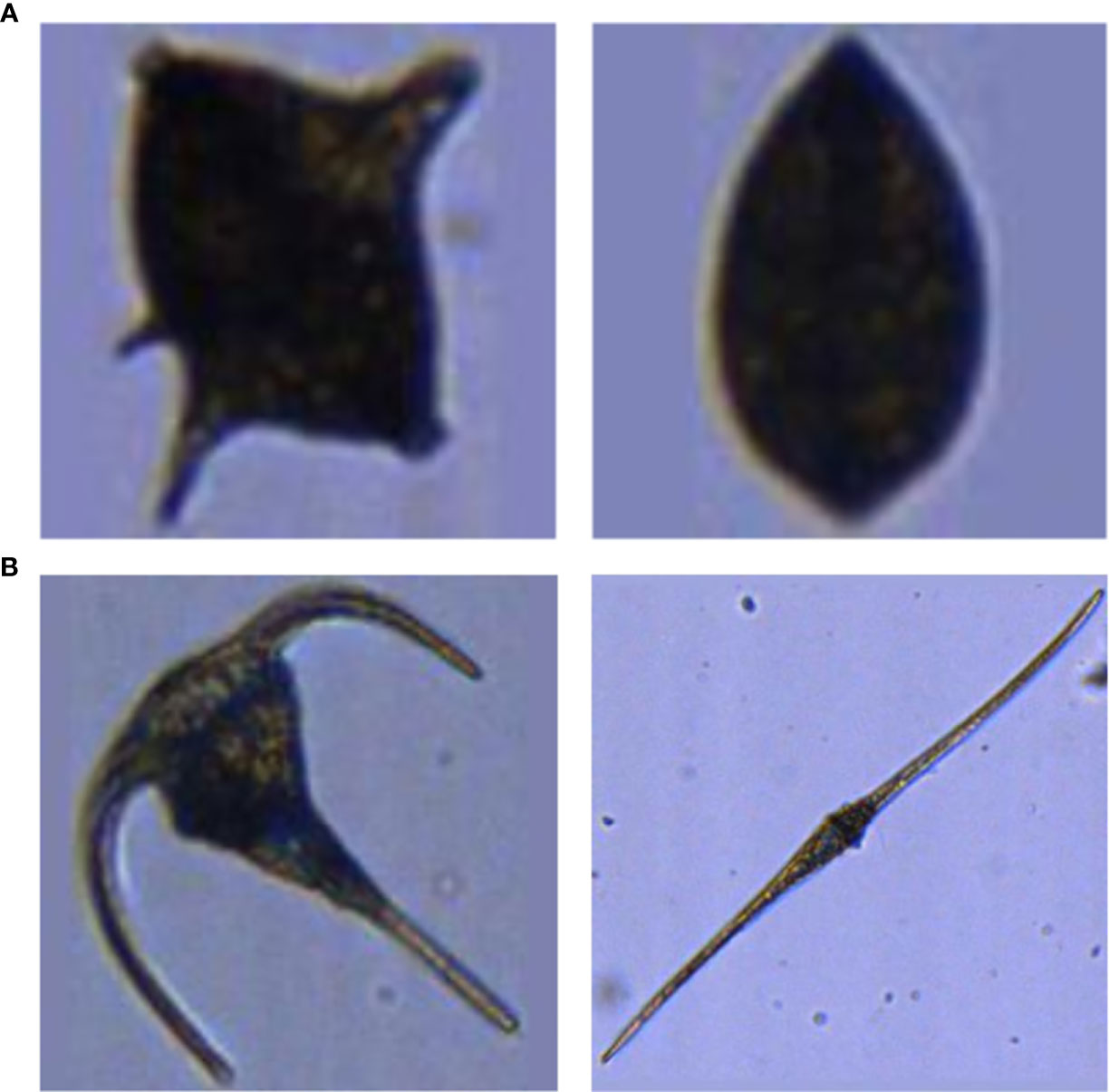
Figure 1 Examples of strong inter-class similarity (A) and high intra-class dissimilarity (B). (A) A dinoflagellate of the genus Protoperidinium spp. (left), and a juvenile bivalve (right). (B) Two dinoflagellates: Ceratium fusus (left) and Ceratium tripos (right).

In summary, the current constraints on successful training and application of models for automatic plankton classification are the often limited quality of training sets, and the high spatio-temporal dynamics of the plankton community. Under these circumstances, manual validation and correction of the model results is recommended (Gorsky et al., 2010), as is the adaptation of the model to avoid a decrease in classification performance. The latter usually requires the availability of machine-learning expertise, a commodity often lacking in the marine sciences (Malde et al., 2020). Research and development should thus be focused on reducing the time required for the validation task and on improving operability of classifier models by non-AI-experts.

Here, we follow González et al.’s (2016) suggestion and propose a pipeline for alleviating the task of model adaptation to a changing plankton community, and thus for reducing the time for manual validation: A “dynamic optimization cycle” (DOC) for iterative use accessible by non-AI-experts. By making applied use of a trained model on field samples, correcting the classification and evaluating model performance through expert knowledge, and updating the model training set and the model itself (through training on the updated image set), the classifier model adapts to spatial and/or temporal changes in the plankton community. It thus maintains high classification performance, ensuring that validation workload remains relatively constant. The systematization of this procedure, and the implementation of the DOC as an end-to-end application with graphical user interface, removes the requirement for expertise in designing and coding CNNs. The DOC was designed for the classification of FlowCam images and the workflow related to studies using the FlowCam, but is likely applicable for other types of plankton images and different types of workflow, as well.

Materials & Equipment

Hardware and Software Requirements

Training of NNs was performed with a Nvidia^® (Santa Clara/California/US) Quadro P2000 GPU with 4 GiB RAM (driver version 410.79) on a Dell^® (Round Rock/Texas/US) Precision 5530 notebook with 32 GiB RAM. CUDA^® (Nvidia, Santa Clara/California/US) version 10.0.130 was used for enabling the GPU to be used for general purpose processing. Programming was performed in Python 3.6.8 (van Rossum, 1995) using the Spyder Integrated Developer Environment (Raybaut, 2017) with Ipython version 7.2.0 (Perez and Granger, 2007). Packages used for analyzing classification outputs included NumPy (Oliphant, 2006), pandas (McKinney, 2010) and Dplython (Riederer, 2016). Packages used for image pre-processing included Matplotlib (Hunter, 2007), PIL (Lundh and Ellis, 2019) and Scipy (Oliphant, 2007). Tensorflow 1.12.0 (Abadi et al., 2015) and Keras 2.2.4 (Chollet, 2015) (with Tensorflow backend) Advanced Programming Interfaces were used for building, training and application of the classifier models.

Methods

Model Design and Training

A convolutional neural net (CNN) was built based on the publicly available “VGG16” network architecture (Simonyan and Zisserman, 2015). This architecture consists of 13 convolutional layers, i.e. 13 intermediate data representations in the form of a stack of matrices that account for positional relationships between pixels of the input image. These layers are arranged in five “blocks” of two-to-three layers each, which are connected via non-parameterized information-pooling layers. The sixth block consisting of so-called “dense” layers was removed – as is usually done when applying a pre-defined architecture – and replaced with custom layers: one convolutional layer and two dense layers. The design of this custom “block” of layers - i.e. the number and type of layers, and the number of neurons (i.e. representation dimensions) of each – was the result of a try-and-error approach for achieving satisfying classification performance on training and validation images (Conradt, 2020). Details on the custom layers can be obtained from tab. SI V/2.

Model parameters were initialized with the values provided together with the VGG16 architecture trained on ImageNet data (Deng et al., 2009) for the respective part of the model, and with values drawn randomly from a Glorot uniform distribution (Glorot and Bengio, 2010) for the custom layers, as per default in the Keras software. Model training (i.e. fitting) was started with the custom layers and the final block of convolutional layers of the VGG16 “base” set to trainable. Training was performed by feeding all training images in a sequence of batches of 20 randomly chosen images to the model. All other hyper-parameter settings (e.g. optimizer and learning rate for gradient-based fitting) can be obtained from Tab. SI IV/1. The choice of hyper-parameter settings was based on a series of trial runs for different hyper-parameter set-ups (Conradt, 2020).

The entire set of training images was fed eight times (so-called “epochs”) to the model, with an increasing number of the layers of the VGG16 base being set to trainable (“unfrozen”) each epoch (Tab. SI V/1). “Unfreezing” is a common procedure applied to ensure that learned features are gradually adapted towards our plankton dataset (VGG16 was originally trained on the ImageNet set of everyday-object images). The chosen number of epochs and the “unfreezing” schedule resulted from optimization through trial-and-error experimentation, as well (Conradt, 2020).They resulted in a steady increase of validation accuracy from approx. 88% to approx. 94% (Figure SI VIII/1 B) and a decrease of validation loss from approx. 0.34 to approx. 0.29 when trained on the baseline training set, though validation loss did increase slightly from a minimum value of approx. 0.26 at the third epoch (Figure SI VIII/1 A). Validation accuracy was surpassed by training accuracy by the second epoch, which is usually a sign of an onset of over-fitting (e.g. Chollet, 2017); however, the fact that validation accuracy also still increased over the eight epochs was taken as a sign of a robust training schedule.

We did not utilize data augmentation, a technique in which artificial transformations are randomly applied to the training data to reduce model over-fitting and thus improve its generalizability (e.g. Chollet, 2017). While the approach is frequently applied in various image-classification tasks (e.g. Luo et al., 2018; Plonus et al., 2021), previous work had shown that data augmentation did not markedly improve the classification when applied to a partly identical data set of FlowCam images (Conradt, 2020). This observation has also been made in another instance on an independent plankton data set (Lumini and Nanni, 2019).

While both the set-up of the CNN and the training scheme may not represent an optimal configuration (for example, over-fitting occurred in our experiments), we found the configurations to yield consistently robust results that were sufficient to support routine plankton analysis work. Given the relatively high validation accuracy, our goal was not to further optimize model design or –training, but instead to maintain this satisfactory performance level over changes in the composition of plankton samples.

Image Characteristics

Input image size was set to 120 x 120 x 3 pixels. A size of 256 x 256 x 3 pixels is more commonly used for plankton images (e.g. Orenstein and Beijbom, 2017; Al-Barazanchi et al., 2018; Cui et al., 2018), however preparatory work for the present study had shown that the chosen image size yielded better performance than a larger size, and leads to a faster processing due to the lower data dimensionality (Conradt, 2020). The use of a common square image shape leads to an altered visual appearance of plankton organisms if the original image had a height-length ratio very different from 1. This would increase intra-class variability, an undesirable trait as described above. Therefore, within the DOC pipeline, images are pre-processed via padding, i.e. by adding pixels in background color (the mode pixel value of the outermost pixel row for each color layer) to the sides or top and bottom to achieve square format, a common procedure in plankton-image classification (see e.g. Plonus et al., 2021).

Characteristics of the Baseline Training Set

The baseline image dataset, which is updated as part of the adaptive procedures of the DOC pipeline, consists of 27900 RGB FlowCam images of plankton samples gathered from various North Sea surveys over several years. Images in the dataset were sorted into 15 classes, including 13 taxonomic groups as well as a detritus class and a “clumps” class that contains aggregates of plankton organisms and/or detritus. The distribution of images over classes was designed to reflect general, though not empirically determined, patterns of natural relative abundance. However, the very abundant detritus class was reduced in relative proportion in order to avoid the learning of a quasi-binary classification scheme (detritus/non-detritus) by the classifier model. A random 80% of images of each class were used as training images for the baseline model, while 10% each were reserved for validation and testing purposes (see above). The characteristics of the baseline data set are given in Tab. SI VI/1.

Classification Thresholds

Within the DOC pipeline, the model classification is compared with expert validation. For each class, the relative amount of correct predictions is calculated and used as a threshold value against which the maximum probability value of the CNN output vector (the index of which is the class prediction) is compared. Probability values above the threshold lead to acceptance of the classification, as the model classification is deemed “certain”. Probability values below the threshold lead to rejection of the model classification, the image is then assigned to an “uncertain-classifications” category. Initially, thresholds were set to 60% for all classes, as the difference between the properties of the baseline training set (on which the baseline model was trained) and the properties of the first station to be classified was deemed to be larger than that between subsequent modified training sets and stations.

This procedure was intended to speed up manual validation by implementing a sort out of images based on probability of miss-classification, which can then be checked more easily than if they were not separated from images with high probability of correct classification.

DOC Pipeline Procedures

The following describes the working steps for applying the DOC onto any given set of plankton samples (see also Figure 2). A more thorough user instruction with technical notes of importance is provided in the appendix (SI 1).

1. Classification (Figure 2A): The DOC pipeline is typically started by applying the provided classifier model directly on the classification of plankton samples, thus allowing for potentially large initial classification error. However, it is also possible to directly train a custom classifier model if the user has already generated a training set from manually labeled images, and perform the classification with this custom model (for details see SI 1).

2. Validation (Figure 2B): Following the classification of two to three plankton samples, the model classification is validated by a plankton expert (by moving images between class folders into which the images were copied by the DOC application). The number of samples required before continuing with the adaptation steps is likely case-specific and might require some initial trial-and-error experimentation. In our case studies, we classified two samples at a time. The validated classification is used as the final classification for further ecological studies. Model classification and expert validation are automatically compared and the correct-classification rate determined for each class.

3. Training-set update and threshold reduction (Figure 2C): After expert validation, the original model training set is stocked up with images that were miss-classified by the model. To this end, first the complement of the correct-classification rates is normalized via division by the maximum miss-classification rate over all classes (eq. 1, top). These values are then multiplied by the number of miss-classified images of each class to determine the number of images to be added to the training set (eq. 1, bottom). Not selecting all miss-classified images reduces the over-proportionality of naturally-abundant, but well-classified classes, e.g. detritus, in the image supplement, putting more emphasis on poorly-classified classes. The images added are selected randomly.

FIGURE 2

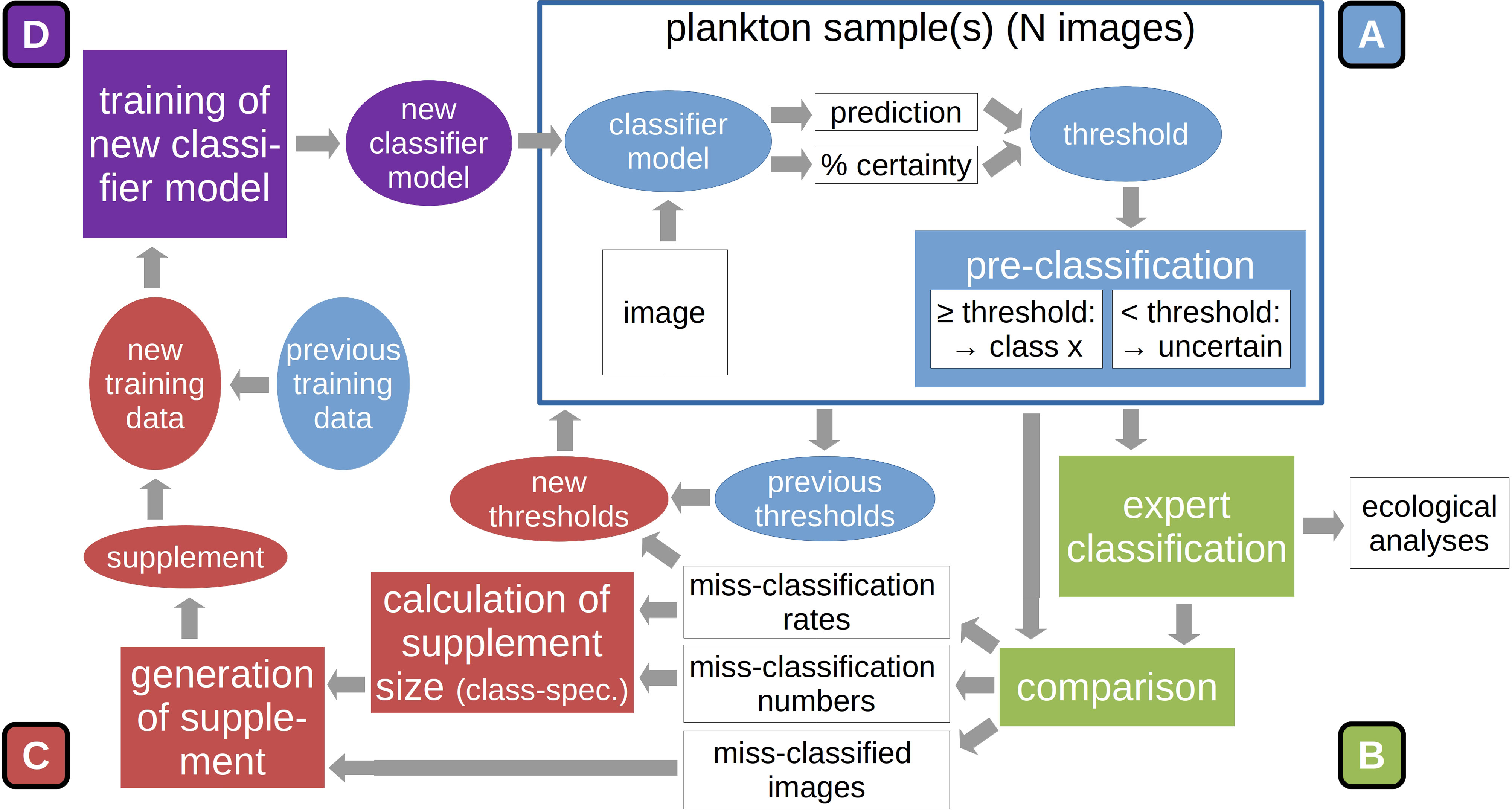
Figure 2 Sequence of main procedures in the DOC pipeline: After the automatic classification (A) and expert validation of a set of plankton samples (B), the original model training set is stocked up with a selection of miss-classified images, based on class-specific miss-classification rate. This constrained update reduces the dominance of naturally-abundant classes in the add-on set. Also, classification thresholds used in automatic pre-classification are reduced based on miss-classification rates (C). A new classifier model is trained on this updated training set. The new model is used to classify the next set of plankton samples (D). Further details are given in the text.

$$\begin{array}{l}{p}_i=\frac{1\frac{C_i}{N_i}}{\text{max}(1-\frac{C_j}{N_j}forj∊class1\dots classn\})}\\ A_i=F_i{p}_i\end{array}$$

Eq. 1: Calculation of the proportion of miss-classified images to be added to the updated training dataset (top) and calculation of the number of images to be added to the training set (bottom). i = index for classes, p = proportion, C = number of correctly classified images in a given class, N = number of images assigned by expert to that class, A = number of images to be added to the training set, F = number of miss-classified images

The class-specific training-set update is the first part of the adaptation procedure. A marked increase in the abundance of a class that was underrepresented in the previous training set will lead to that class being better represented in the adapted version. As a second adaptation step, the previous threshold values for automatic culling of likely miss-classified images (see Classification Thresholds) are multiplied with the correct-classification rates. This reduces the threshold percentage above which a classification will be deemed correct for classes that receive an increase in training images in the first adaptation step. It is assumed that large threshold values reduce classification performance by the assignment of many in fact correctly-classified images to the “uncertain-classifications” category. By decreasing the classification threshold, the number of images correctly assigned to the predicted classes can theoretically be increased, leading to higher correct-classification rates.

4. Model training (Figure 2D): The model is then trained on the updated training set according to the training schedule described above. It should be noted that a completely new model instance is generated and trained. This is done to avoid an over-adaptation of the model on the training data, since re-training would mean training the existing model for an additional set of epochs on a still partly identical training set (no original training images are dropped during training-set updates).

After training is completed, the new model can be applied on the next batch of plankton samples, and the adaptation cycle continues anew. The DOC was devised on the notion that plankton communities change on a spatial and/or temporal gradient. It therefore makes sense to process the plankton samples in the same order as they were taken by the research vessel (or along hydrographic gradients).

Further notes on the DOC procedures can be found in SI VII.

User Application

A user application with graphical user interface was designed to aid in the implementation of the DOC pipeline. For practical purposes, it is intended that the DOC pipeline be implemented by a broad user group not necessarily familiar in the use of programming languages and/or Machine-Learning techniques. The DOC application was therefore designed to enable an end-to-end implementation of all pipeline steps described above. It consists of a series of executable, partially nested, Python scripts, one executable Bash (GNU Project, 2007) script that accesses the Python scripts and a comprehensive instruction guide describing the implementation of all DOC-pipeline steps in the application context (SI 1). None of the scripts is protected, which allows users familiar with the Python programming language to edit and change scripts in order to make custom changes to the pipeline processes, if desired.

The DOC application was written in the Python programming language, making extensive use of the TkInter package for graphical-user-interface design (Lundh, 2019) and of the os package for file-system access. One script utilized to start the application was written in the Bash command language.

The DOC application was designed for use on Linux (The Linux Foundation, San Francisco/CA) operating systems (tested on Ubuntu 18 and Linux Mint 19). It requires hardware and drivers enabling the training and application of Deep Neural Networks for image classification. For the application development and for conducting the case studies, a Nvidia^® Quadro P2000 graphics-processing unit (GPU) was utilized. Further system details are given in SI II. The DOC application requires the installation of Python 3 (was tested under Python 3.6) via the Anaconda (Anaconda Software Distribution, 2020) distribution, and the creation of a dedicated Python environment containing i.a. the packages Tensorflow (Abadi et al., 2015) and Keras (Chollet, 2015). Full details on the environment setup are given in SI III.

The DOC application is started via the Bash script, whereupon each of the DOC processes can be started. The single processes can be executed in the order described above and suggested in the instruction manual, but can also be executed singularly, e.g. when only image classification, but not the implementation of the full DOC pipeline is desired.

The DOC user application, including the baseline training set, is available on zenodo.org (doi: 10.5281/zenodo.6303679).

Case Studies – North Sea Surveys

The DOC pipeline was applied to samples taken on two plankton surveys in order to test the performance of the approach.

The surveys were conducted in autumn and winter 2019 in the Western North Sea. The first survey, undertaken in September 2019, started offshore the East Coast of Scotland at approx. 57.5°N/0°E, and moved gradually closer to the British coast in a zig-zag trajectory between approx. 56.2°N and 57.5°N (Figure 3A). Samples were taken at these two latitudes and at approx. 57.9°N. The second survey was conducted in December 2019 in the English Channel, starting at the eastern entrance of the Channel at approx. 51.6°N/2°E, continuing south-westwards until approx. 50.25°N/-1°E, and changing direction north-east-wards, for a route parallel to but closer to the French coast than the initial trajectory (Figure 3B). Plankton samples were taken with a PUP net (mesh size: 55 µm) attached to a GULF VII sampler (HYDRO-BIOS Apparatebau GmbH), which was towed in double-oblique hauls.

FIGURE 3

Figure 3 Survey transects and location of the sampling stations from the September (A) and December (B) surveys.

Plankton samples were stored in 4-%-formaldehyde-seawater solution. Once in the laboratory, samples were processed using a FlowCam, following the FlowCam^® Manual V 3.0 (Fluid Imaging Technologies, 2011). The FlowCam flow chamber had a depth of 300 µm, which was also the maximum size of plankton particles processed by the apparatus (the minimum particle size was determined by the PUP net mesh size of 55 µm). Flow rate was set to 1.7 mL min^-1, in order to achieve high image quality at an acceptable processing speed. Using the AutoImage mode of the FlowCam’s Visual Spreadsheet software, images were saved for later processing.

For both surveys, the DOC pipeline was implemented for the classification of 18 samples, with the samples being processed in the sequence they were taken at sea (one sample was taken at each station). The processing sequence equals a spatial and temporal trajectory through plankton habitat. The adaptation procedure was implemented every second station, pooling the images for both stations in order to calculate the misclassification rate and to supply the information for the update of the training set. Classification performance was then calculated for each pair of stations (see below), which in the end yielded a performance trajectory over the survey samples and adaptation steps. Each mark on the trajectory thus constituted the performance of one specific model (trained on one specific version of the training set) applied to one specific set of images. In the Machine-Learning context, this information yielded the test performance of the models at the different adaptation steps, i.e. and indicator of their performance on non-training images under constant field conditions (e.g. Chollet, 2017).

In order to assess the importance of the continuous adaptation, a set of reference runs was performed: After each adaptation step, the current model was saved, and all subsequent samples were classified with this model (previous samples were not classified, as images contained in these were introduced into the training set during previous adaptation cycles). This way, we generated a set of reference classification trajectories in which adaptation is stopped after various numbers of samples processed (and thus on different points of the survey trajectory). This set was used to assess the value of continuous adaptation of the training set and the training of new models thereon: By comparing the performance of an adapted model to a non-adapted or less-adapted model at a specific mark on the classification trajectory, the value of adaptation could be determined for a specific sample or point on the survey trajectory. Integrated over all samples, this allowed evaluating the performance of DOC-based adaptation over the survey-/adaptation trajectory, with respect to overall advantage and potential temporal dynamics in the magnitude of adaptation advantage.

With eight adaptation steps, nine different classification trajectories resulted in total: The fully-adaptive pathway (with one adaptation cycle and the usage of a new model every second station), and eight pathways in which adaptation was stopped at a specific station (Figure 4).

FIGURE 4

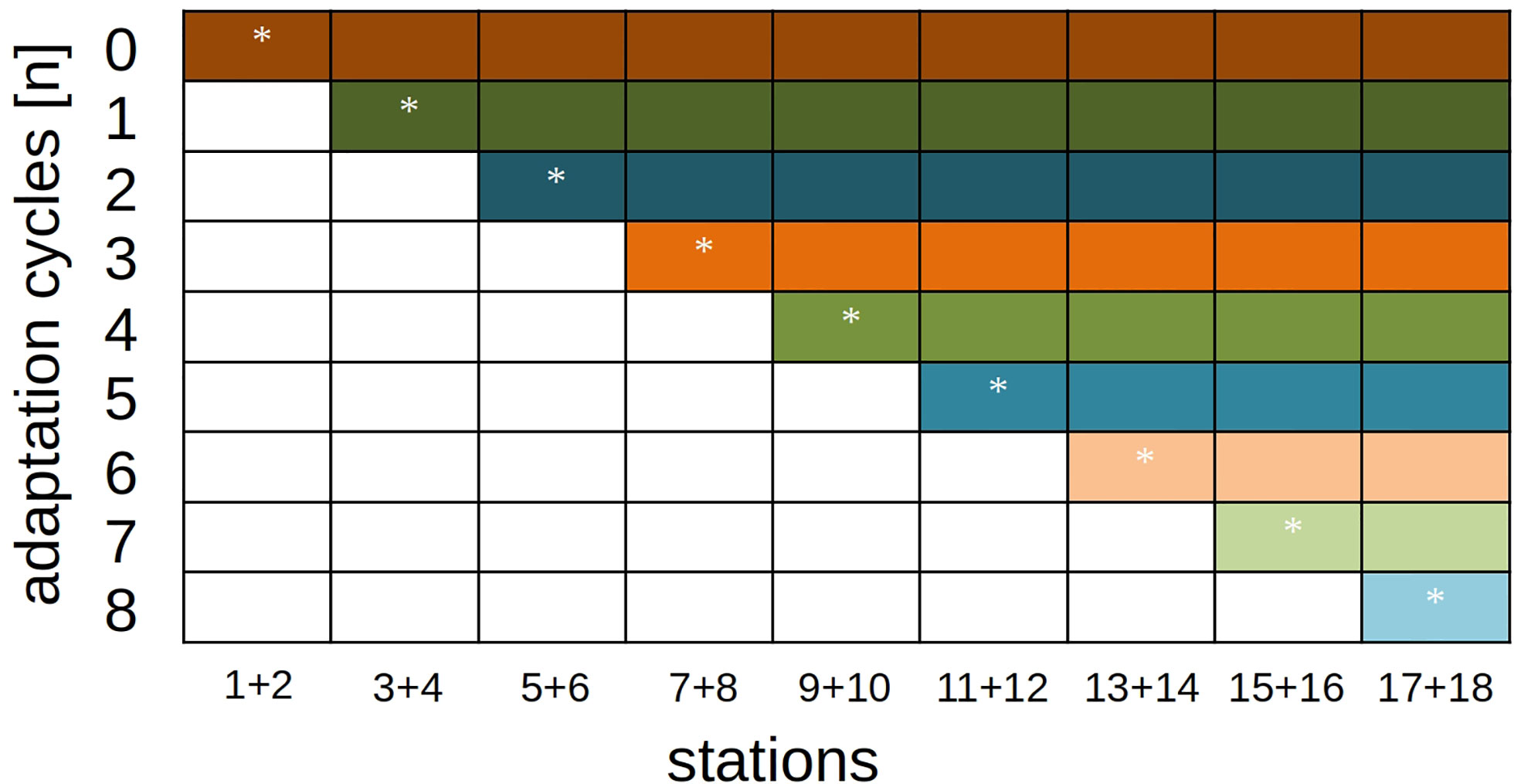
Figure 4 Model-adaptation/station-classification schedule for performance analyses. The diagonal row (marked with stars) represents the fully-adaptive implementation of the DOC pipeline, where an adaptation is implemented every second station. All colored rows show reference runs where samples are classified with an existing model and without further adaptation.

We implemented the adaptation pathway twice for each survey to account for random effects in the adaptation procedure, generating two replicates each. These primarily include the parameter initialization before training of every model (i.e., at every adaptation step) except the base model (which was always identical) and the selection of miss-classified images for the updating of the training dataset.

We calculated recall and precision to analyze classification performance on overall- and class level, as well as cross-entropy to assess the ability to predict the plankton-community composition (see Box 1 for details). We compared cross-entropy with class-specific differences between true and predicted relative abundance to analyze the driving factors behind changes in cross-entropy. Means and standard deviations weighted by class abundance of recall and precision were calculated for each pair of stations and each adaptation trajectory. Recall and precision values for “detritus”, “clumps” and “uncertain predictions” classes were not included in the calculations of averages in order to focus on the living components of the plankton (which are the target of plankton research). More specifically, miss-classification of detritus is of little concern in research focusing on living biomass, and clumps are miss-classifications per se, since a researcher would need to analyze clumps compositions manually nevertheless. The three classes were excluded from calculation of average precision, as the direct aim of achieving high precision is to reduce the effort of removing miss-classified images from a given class folder. Since detritus, clumps and uncertain classifications are not directly of interest in plankton research, the desire to achieve “clean” folders for these classes is comparatively low. These classes were also excluded from calculating cross entropy due to them not representing biological taxa.

Box 1. Metrics for the analysis of classification performance
Recall: Recall is the class-specific ratio of correctly-classified images (true positive classifications) to the total number of images (true positive plus false negative classifications), where the total number is defined by the expert classification (eq. B1, top). This metric indicates the expert effort required to find miss-classified images in all other class folders.

Precision: Precision is the class-specific ratio of correctly-classified images (true positive classifications) to the sum of correctly-classified images (true positive classifications) and miss-classified images (false positive classifications), where the total number is defined by the expert classification (eq. B1, bottom). This metric indicates the expert effort required to find all images that were mistakenly assigned to a specific class folder

$$recall=\frac{n\left(true positive\right)}{n\left(true positive\right)+n\left(false negative\right)}$$

$$precision=\frac{n\left(true positive\right)}{n\left(true positive\right)+n\left(false positive\right)}$$

Eq. B1: Definitions of recall and precision (class-specific metrics)

Categorical cross entropy: Categorical cross entropy (hereafter referred to simply as “cross-entropy”) measures the loss between a true and a predicted distribution (eq. B2). This metric is calculated from the true (derived from expert classification) and the predicted (derived from model classification) relative class abundances. Cross-entropy measures the goodness of predicting the quantitative plankton-community composition. In the present study, for classes with a predicted relative number of zero, this value was set to one divided by the total number of images in a given sample (the cross-entropy is not defined for data including zero-values; hence, one correct classification is introduced, which we assume to be a plausible stochastic error given numbers of images per sample of usually more than ten-thousand).

$${\gamma }_i=-{\displaystyle \sum _{i=1}^{N_c}{a}_{i}log\widehat{a_i}}$$

Eq. B2: Categorical cross entropy (γ). a = true relative abundance, â = predicted relative abundance, N_c = number of classes

Cross-entropy represents information loss between true and predicted distributions, which makes it difficult to interpret single values. Therefore, the metric is used exclusively for comparative purposes (e.g. for comparing different models) in the present study.

Analyses and visualization were performed in R version 3.6.3 (R Core Team, 2020), partially using the packages “tidyverse” (Wickham et al., 2019), “viridis” (Garnier, 2018) and “radiant.data” (Nijs, 2020).

Results

Overall performance in the fully-adaptive mode of the DOC was relatively high with regard to recall, with weighted means ranging between approx. 82 and 92% over all survey-station pairs. Precision was lower, with weighted means ranging between approx. 50-75% for the September survey, and approx. 60-80% (with one very low value of 30% at start) for December. Performance was sufficiently large to enable successful usage of the DOC application in the context of experimental research work, which benefitted from the time-savings through semi-automatic classification and model adaptation (Börner, unpubl. data).

Altogether, a fully-adaptive implementation (adaptation cycle implemented every second station) of the DOC frequently achieved comparatively high or top level mean performance in recall and precision metrics, though absolute and comparative performance varied between both survey month, and, more strongly, between classes (for details see below). Performance gains were often largest in the first one to two adaptation cycles, i.e. after the first adaptation of the baseline training set.

Recall

Overall, there were no clear trends in mean recall development over stations for the larger part of the classification trajectory, neither in the fully-adaptive nor in the less-adaptive implementations (Figure 5): In the September trajectory, mean recall for the fully-adaptive mode decreased from approx. 90% by approx.10% after the third station pair (stations 5 and 6), and increased again somewhat after stations 11 and 12 in both replicates (Figures 5A, B). Mean recall at stations 17/18 was approx. 91%. In the December trajectory, mean recall for the same mode increased strongly between stations 3/4 and stations 5/6, from approx. 20% to slightly over 90% in both replicates (Figures 5C, D). Recall remained at a relatively high, though slightly decreasing level, having a final value of approx. 85% at stations 17/18.

FIGURE 5

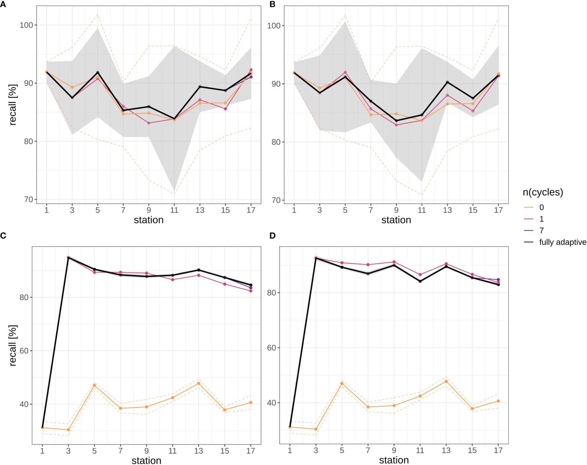
Figure 5 Recall trajectories for different modes of adaptation using the DOC. Solid black line represents weighted mean of the fully-adaptive implementation, grey area denotes the corresponding weighted standard deviation. Colored solid and dashed lines represent weighted mean and weighted standard deviation of less-adaptive implementations (denoted by the number of adaptation cycles). (A): September survey, first replicate, (B) September survey, second replicate; (C): December survey, first replicate, (D): December survey, second replicate. Replicates differ in the random selection of images for training-set updates and random parameter initializations of models before training (see Case Studies – North Sea Surveys). Trajectories for all nine adaptation modes are shown in Figure SI XI/1. Note that weighted standard deviation for the fully-adaptive implementation in the December survey is very small compared to that in the September survey.

Relative performance to less adaptive DOC implementations differed initially strongly between the two surveys, but became more similar thereafter. While in the September samples no large performance difference was visible between the adapted and the baseline model at stations 2/3 (Figures 5A, B), recall for the more adaptive model strongly outperformed that of the less adaptive one in the December samples, as a value of over 90% was achieved with the former, while no marked performance difference to the first station (approx. 20% mean recall) was detected in the latter (Figures 5C, D). With the exception of the baseline model used for the December samples, which remained at low-level performance of approx. 40% mean over the trajectory, recall of the fully-adaptive mode was not markedly superior or even somewhat inferior (in the December samples) to that of less adaptive approaches, depending on the replicate. Performance of all adaptive modes converged to a relatively similar value (approx. 91%) in the final September sample (see also Figure SI XI/1). Convergence was not present in the December samples.

Recall trajectories differed strongly between classes, and showed stronger fluctuations between station pairs than the weighted mean trajectory over all classes, with values of zero and 100% being reached occasionally (Figures 6, SI XI/2). Trajectories for the fully-adaptive implementation of the DOC were relatively similar between replicates, though (compare Figure 6A vs B, and Figure 6C vs D). For many classes, a recall of markedly over 90% was achieved at least occasionally in fully adaptive mode, although the identity of these classes differed between September (Figures 6A, B) and December surveys (Figures 6C, D). Classes for which a relatively high recall was frequently achieved (though not necessarily consistently over all stations) included Ceratium spp., Protoperidinium spp. (September survey only), copepods, detritus and diatoms. All other classes showed relatively high performance at least once in the recall trajectory; thus it is not possible to name classes for which recall was particularly poor. The comparative performance of the fully-adaptive implementation of the DOC varied strongly between classes, as well. Furthermore, performance also varied between surveys, and to a smaller extent between replicates. For some classes, such as bivalves (September), detritus (both surveys), diatoms (both surveys), dinoflagellates (September), foraminiferans (September), unknown taxa A, B and C (only present in September), as well as copepods (December), the fully-adaptive implementation yielded near- or top-level performance over the larger part of the stations trajectory. For other classes, including copepods (September) and Dinophysis spp. (September), comparative performance was relatively constantly poor. It should be noted that performance differences between different modes of adaptation were of various magnitudes between classes. In most classes, the recall trajectory of the fully-adaptive implementation followed the general trend shown by all modes of adaptation.

FIGURE 6

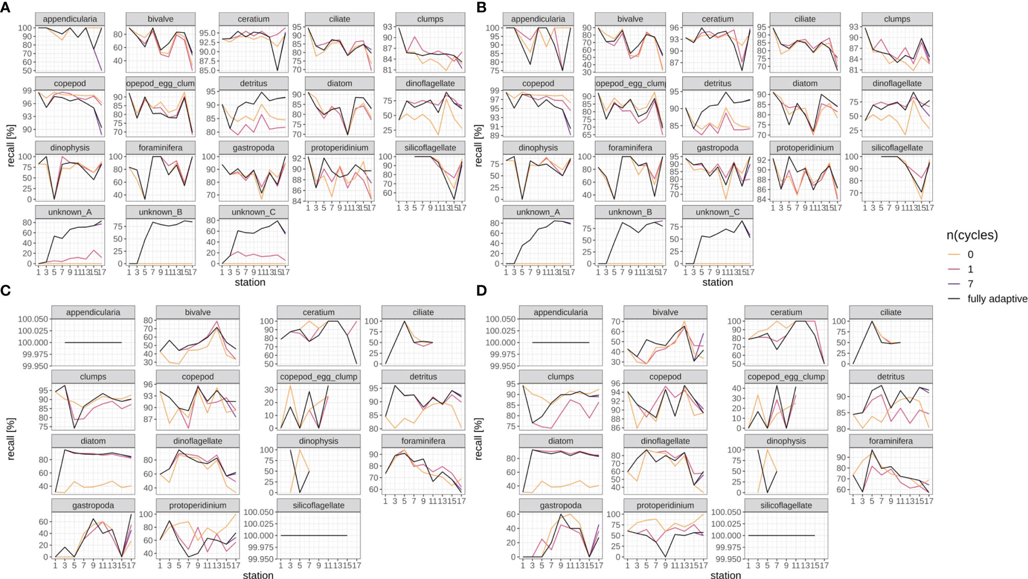
Figure 6 Class-specific recall trajectories. Black line represents fully adaptive DOC implementation (training-set update every second station); colored lines represent less-adaptive implementations (denoted by the number of adaptation cycles). (A): September survey, first replicate, (B) September survey, second replicate; (C): December survey, first replicate, (D): December survey, second replicate. Replicates differ in the random selection of images for training-set updates and random parameter initializations of models before training (see Case Studies – North Sea Surveys). Trajectories for all nine adaptation modes are shown in Figure SI XI/2.

Precision

In general, mean precision increased in both survey trajectories slightly, in all but the two least adaptive implementations of the DOC after a more variable initial phase (first two station pairs) (Figure 7). Mean precision increased from approx. 60% at stations 5/6 to approx. 75% at stations 15/16 in the September survey in both replicates (Figures 7A, B), and from approx. 65% to approx. 80% in the December survey in both replicates (Figures 7C, D). Mean precision then decreased again from stations 15/16 to station 17/18, from the mentioned values to approx. 63% in the September survey, and to approx. 70% in the December survey. Altogether, the trajectory of mean precision was smoother for the December survey, i.e. there was little fluctuation between adjacent station pairs.

FIGURE 7

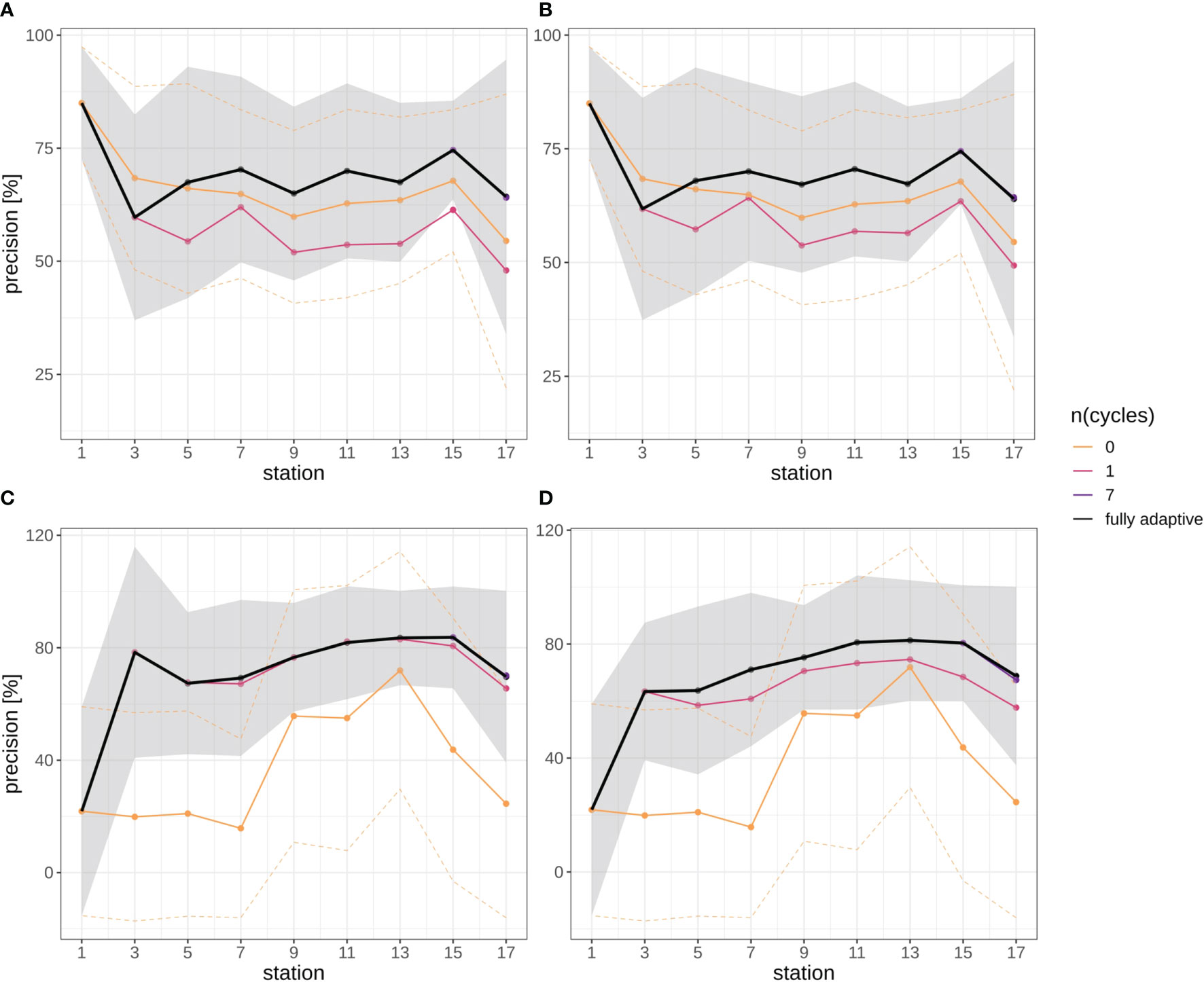
Figure 7 Precision trajectories for different modes of adaptation using the DOC. Solid black line represents weighted mean of the fully-adaptive implementation, grey area denotes the corresponding weighted standard deviation. Colored solid and dashed lines represent weighted mean and weighted standard deviation of less-adaptive implementations (denoted by the number of adaptation cycles). (A): September survey, first replicate, (B) September survey, second replicate; (C): December survey, first replicate, (D): December survey, second replicate. Replicates differ in the random selection of images for training-set updates and random parameter initializations of models before training (see Case Studies – North Sea Surveys). Trajectories for all nine adaptation modes are shown in Figure SI XI/3.

Different from the recall trajectories, mean precision of the fully-adaptive mode of the DOC was frequently at top level compared to less-adaptive modes, in both the September and the December survey (for almost every station in the latter; Figures 7C, D) (see also Figure SI XI/3). The zero-adaptive implementation (use of the baseline model for all classifications) showed markedly lower performance than all other implementations over the full trajectory in the December samples, while lowest performance was achieved by the one-time-adapted model in the September samples. In the latter case, the performance difference was not as pronounced as in the September samples, though. While mean precision for the weakest-performing mode was relatively constant to slightly decreasing in the September survey (approx. 55% at stations 5/6 to approx. 50% at stations 17/18), it did temporarily increase from stations 7/8 to a peak at stations 13/14 (from approx. 20% to approx. 75% to approx. 25% at stations 17/18) in the December survey.

Precision trajectories differed strongly between classes and surveys (Figures 8, SI XI/4), but were mostly consistent between replicates (compare Figures 8A vs B and Figures 8C vs D), both with regard to the fully-adaptive implementation of the DOC and to its comparison with less-adaptive implementations. For most classes, precision varied strongly between adjacent stations, and did not bear a clearly increasing or decreasing trend. For many classes in the September survey (Figures 8A, B), the fully-adaptive implementation achieved near- or top-level performance over the larger part of samples; exceptions include the “clumps” class, copepod egg clumps, detritus, dinoflagellates and the two unknown taxa “A” and “B”. However, unlike in the case of class-specific recall, a comparatively poor or very poor performance was observed for none of these exceptions. In the December survey (Figures 8C, D), the fully-adaptive implementation achieved average performance for the larger number of classes. Exceptions with near- or top-level performance over the larger part of the trajectory include bivalves, Dinophysis spp., foraminiferans and Protoperidinium spp.; for few additional classes, top-level performance was achieved in only one of the two replicates. Very poor performance was also noted for a few classes (appendicularians, copepod egg clumps, gastropods), but again only in one of the two replicates. As with class-specific recall, performance differences between differently-adaptive modes were of different magnitudes for different classes, and the precision trajectories of the fully-adaptive mode in general followed the trend of all other modes of adaptation.

FIGURE 8

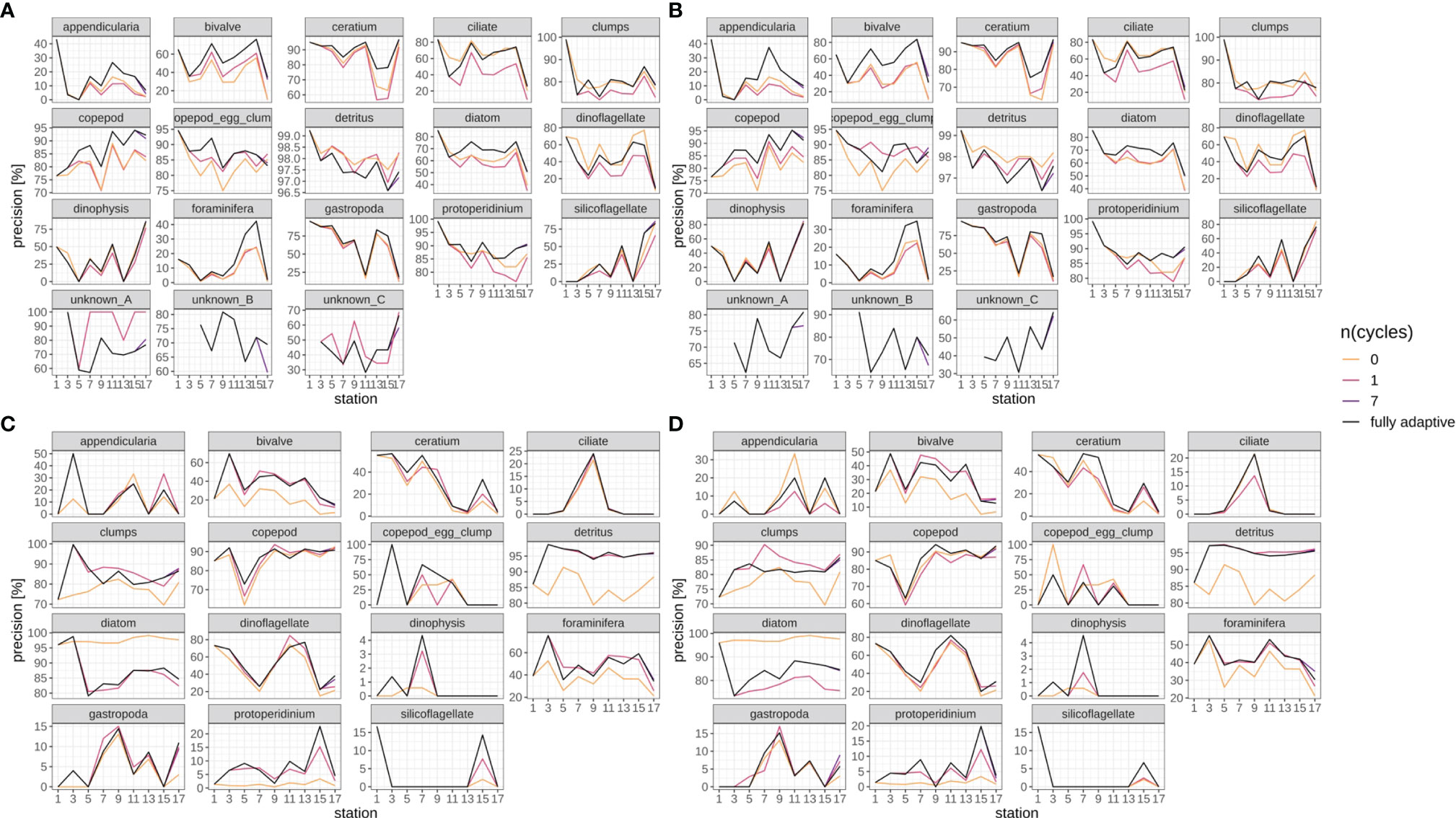
Figure 8 Class-specific precision trajectories. Black line represents fully adaptive DOC implementation (training-set update every second station); colored lines represent less-adaptive implementations (denoted by the number of adaptation cycles). (A): September survey, first replicate, (B) September survey, second replicate; (C): December survey, first replicate, (D): December survey, second replicate. Replicates differ in the random selection of images for training-set updates and random parameter initializations of models before training (see Case Studies – North Sea Surveys). Trajectories for all nine adaptation modes are shown in Figure SI XI/4.

Cross-Entropy

Cross-entropy in general decreased over the stations trajectory, representing an increasing similarity between true (as defined by classification expert) and predicted distributions of relative abundances of plankton classes (Figures 9, SI XI/5). By the end of the trajectory (stations 17/18), cross-entropy of the fully-adaptive implementation was decreased to approx. 90% and 40% of its value at the start of the trajectory for the September and December surveys, respectively. The cross-entropy trajectories were markedly smoother for the December survey (Figures 9C, D) than that for the September survey (Figures 9A, B), which featured an oscillatory pattern from stations five/six onwards. In the September survey, the deviation between true and predicted distributions was driven by a variety of classes, including the constantly strongly abundant diatoms and Protoperidinium spp. classes, as well as the occasionally strongly abundant Ceratium spp. class and the little-abundant unknown taxa “B” and “C” (Figures 10A, B). The cross-entropy decrease was primarily driven by lowered differences between predicted and true relative abundances of the diatoms class and of the two unknown taxa. Differences were not lowered by a large amount; however, the magnitude of absolute differences was not large (<< 10% at maximum). In the December survey, the deviation was almost exclusively driven by the strongly-abundant diatoms class and the little-abundant Protoperidinium spp. class (Figures 10C, D). Cross-entropy decrease was notably driven by a decrease in the difference between predicted and true relative abundance for both classes. Differences decreased by a large magnitude, from more than 50% absolute to markedly less than 20%. Cross-entropy trajectories and deviations between true and predicted abundances were very similar between replicates (compare Figure 9/10A vs B and Figure 9/10 C vs D).

FIGURE 9

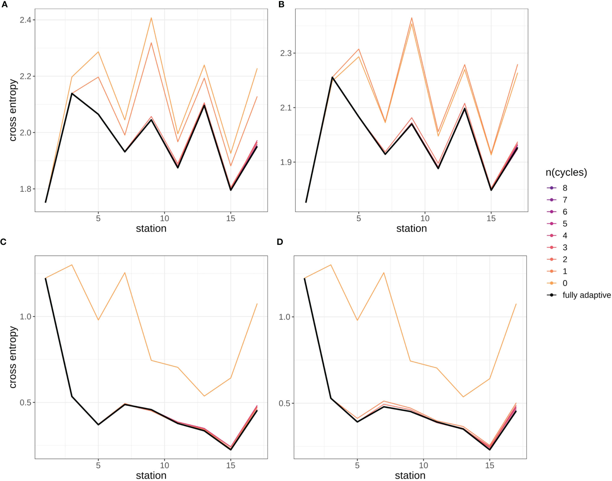
Figure 9 Cross-entropy trajectories for different modes of adaptation using the DOC. Solid black line represents weighted mean of the fully-adaptive implementation, grey area denotes the corresponding weighted standard deviation. Colored solid and dashed lines represent weighted mean and weighted standard deviation of less-adaptive implementations (denoted by the number of adaptation cycles). (A): September survey, first replicate, (B) September survey, second replicate; (C): December survey, first replicate, (D): December survey, second replicate. Replicates differ in the random selection of images for training-set updates and random parameter initializations of models before training (see Case Studies – North Sea Surveys). Trajectories for all nine adaptation modes are shown in Figure SI XI/5.

FIGURE 10

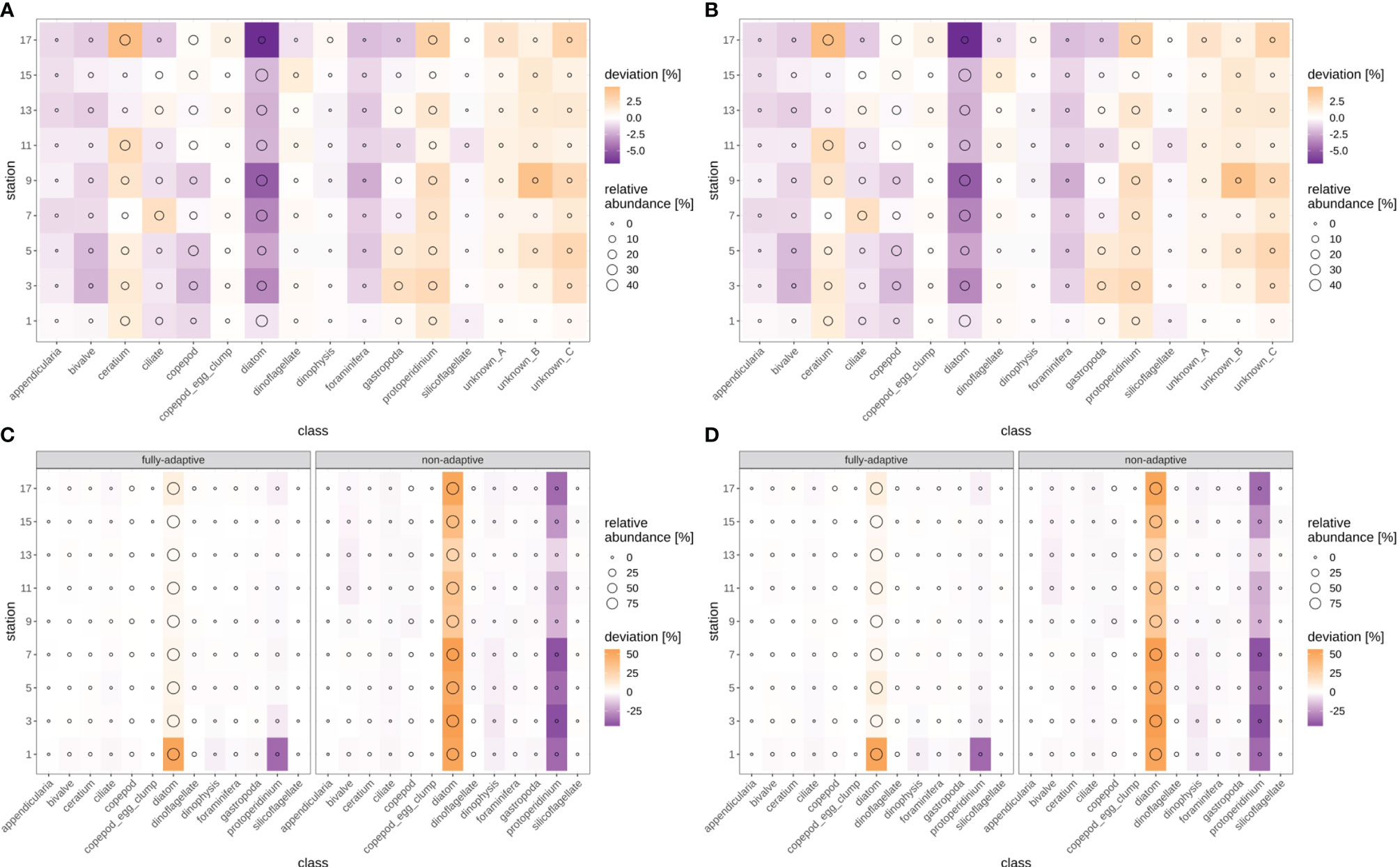
Figure 10 Deviation between true and predicted (via non-validated automatic classification) relative class abundances, for the fully-adaptive DOC implementation and for classification of all samples with the baseline model (no adaptation). Circle size indicates true relative abundance. (A): September survey, first replicate, (B) September survey, second replicate; (C): December survey, first replicate, (D): December survey, second replicate. Replicates differ in the random selection of images for training-set updates and random parameter initializations of models before training (see Case Studies – North Sea Surveys).

Cross-entropy was lowest over all stations compared to all other adaptation modes, in the fully-adaptive implementation of the DOC (see also Figure SI XI/5). It was markedly higher in the two least-adaptive implementations in the September survey, and in the none-adaptive implementation in the December survey, compared to all other implementations. Relative cross-entropy dynamics over time were similar among all adaptation modes.

Discussion

Our results show that adapting a classifier model to changes in the plankton community is vital for ensuring continuously high classification performance. As the comparison between the fully-adaptive and less-adaptive performance trajectories demonstrates, the standardized procedure implemented in the DOC pipeline generates suitable adaptation steps via training-set stock-up and reduction of classification thresholds, making the DOC an appropriate tool for implementing model adaptation

Our results confirm that continuous adaptation via the DOC pipeline clearly improves classification performance compared to more limited or no adaptation. The fact that performance of the classifier model improved over adaptation steps – primarily in comparison to less-adaptive scenarios, but to some extent also over survey stations, with regard to precision and cross-entropy – shows that the DOC is indeed able to cope with and actively learn from a difficult classification task. However, it is worth noting that improvement was not existing or continuous for all metrics and taxa, with e.g. mean recall not showing clear signs of improvement over stations. Given that neural networks generally require large amounts of data for training (Goodfellow et al., 2016), a larger initial training set and processing of larger samples might have yielded a clearer, more universal performance improvement. Still, in the context of field research, where image data from a new region and/or time period may initially be sparse, the DOC pipeline makes effective use of the incoming data such that best possible performance is frequently achieved.

With regard to precision and cross-entropy metrics, the highest possible performance is achieved for almost every sample by the fully-adaptive implementation of the DOC, while recall performance is often at very high comparative levels. The same is true for a number of single taxa that are of strong importance in the study of the ecological function of marine plankton, e.g. in the determination of planktonic biomass available as food to commercially-harvested fish (e.g. Peck et al., 2012). Thus, fully continuous adaptation yields the best performance possible per sample when integrating over all three performance metrics.

It should be noted that the DOC was not designed with the intention of advancing classification performance in terms of improving accuracy on artificially created validation datasets. Rather, the aim was to design a procedure that achieves acceptably good performance for applied research work that focusses on abundant and broad taxonomic plankton groups, and in particular maintains that level of performance even as the classifier model is confronted with changes in the plankton community. Still, with weighted mean recall ranging from 80 to over 90%, the classification performance of our model is comparable to the current state of the art, which ranges approximately between 80 and 95% (Dai et al., 2016; Luo et al., 2018; Briseno-Avena et al., 2020). Although some studies have reported very high accuracies of over 95% (Al-Barazanchi et al., 2018; Cui et al., 2018), this performance metric appears to depend strongly on the diversity of samples and on the classes chosen to report accuracy on (Luo et al., 2018; Briseno-Avena et al., 2020), which makes model comparisons difficult. Compared to recall, precision of our approach is somewhat low at 60 to 80%, but still similar to the 84% reported by Luo et al. (2018).

Given that speed and easiness of adaptation was also deemed critical for applied usage of the model, the DOC omits a thorough sample-specific model optimization (by means of re-designing the architecture of the Deep Neural Network or changing the training scheme), which might have yielded stronger performance. However, trading in performance optimization for performance reliability and easiness of adaptation did not affect the usefulness of the procedure in the particular research application it was designed for (Börner, unpubl. data) and in routine classification work.

Performance trajectories varied strongly between the two surveys, but to a lesser extent between replicates, both with regard to weighted-mean and to class-specific performance in most classes. This demonstrates that the DOC is affected by natural variability in the plankton community rather than by technical random factors (e.g. the sampling of additional training images during the adaptation procedure). In particular, performance appears to be affected by the complexity of the plankton community, as expressed via the degree of homogeneity of relative abundances of the plankton taxa: In the September survey, taxa that made up a very minor part of the total number of plankton organisms of the December samples (e.g. Ceratium spp.) were comparatively increased in relative abundance, yielding a more heterogeneous plankton community. Furthermore, the increase varied between survey stations, creating an additional spatial level of heterogeneity. Consequently, the capacity to correctly predict the distribution pattern over classes, as measured by cross-entropy, became lower, as did the capacity to improve that performance by applying the DOC over several stations. As a result, mean precision was also lower for the September samples, as the increased abundance of non-major classes (for which fewer training images were available) likely led to more miss-classifications that reduced the purity of the model-generated class folders. Given that precision for the September samples increased slightly over stations, and markedly over the number of adaptation steps employed, it becomes visible that the DOC still led to adaptation even in this more difficult classification situation.

The fact that high recall was achieved for the diatom, copepod and some dinoflagellate classes, and that poor precision only occurred in some rather minor classes, makes the DOC useful for research questions addressing abundant plankton taxa. These can include analyses on the amount of potential plankton food available to larval fish, which combine classification with length measurements on the plankton items to calculate taxon-specific biomass estimates (e.g. Menden-Deuer and Lessard, 2000; Kiørboe, 2013). A high classification success on abundant classes thus enables a rapid estimation of the larger part of planktonic biomass, while low classification success on more rare classes does not influence biomass estimation particularly strongly. The distribution of classification performance over classes thus also shows that the DOC is particularly useful for broad quantitative analyses on the plankton community. It is not particularly well suited for qualitative surveys e.g. intended to assess the biodiversity of a certain marine area, which naturally require a classification with higher taxonomic resolution. Still, the DOC can in theory also facilitate expert-based high-level classification, as a performance improvement on a broad taxonomic scale will help the expert to better focus on the finer-scale classification of the taxon of interest. However, this would require the usage of different imaging devices, since FlowCam image resolution only allows for broad taxonomic classification even by experts (sensu Álvarez et al., 2014).

It should be pointed out that the viability of our DOC over longer series of survey samples might not necessarily follow the trends observed on the classification trajectories presented here. While the fact that performance improvements were observed in both the September and December transects indicates stability of the DOC pipeline under various ecological conditions, it remains to be seen how its performance behaves beyond the 18 stations per survey covered here. It is possible that at some point, a manual re-design of the training set might be necessary due to very drastic changes in the plankton community (note that the DOC approach does not discard training images during adaptation, leading to an increase in complexity of the training dataset over samples). Also, the continued decreasing of classification thresholds might at some point prove detrimental to classification precision due to many wrong classifications appearing in class folders instead of the “uncertain-classifications” folder. Some indications of deteriorating performance in the final survey samples (precision in September samples, recall in December samples) were observed in our case study, which might be an indication of the effects mentioned. For applied usage, we suggest to monitor the performance trajectory of the DOC in order to determine whether manual adjustments are advisable. Additionally, depending on the performance level found acceptable and the perceived chance of strong community changes, it may not be necessary to implement the DOC adaptation scheme after each processed sampled. It is up to the user to decide on a good trade-off between the performance improvement achieved through model adaptation and the time saved by not implementing the DOC adaptation steps.

The DOC pipeline proposed by us is not the first attempt at continually maintaining or improving model performance as new plankton samples are classified and validated in applied use: Gorsky et al. (2010) initially made use of a plankton training set not specifically built for their study, and obtained improved classification results once adding validated images from their samples and training a model on this. They continued this procedure until further improvements became marginal. Li et al. (2022) systematized a scheme of human-model interaction, where validated images are added to the training set during applied usage of the classifier. However, neither study has explicitly quantified performance decay nor the effect of training-set updates over a spatial trajectory as presented here. Also, both used expert validation to grow the training set in a rather non-systematized manner, and classification thresholds (to accept or discard a model classification as “uncertain”) were not adapted. While a non-systematized growing of the training set achieved marked performance improvements in both studies, our work shows that careful systematized training-set updates and adaptation of classification thresholds initially improve and then maintain classification performance without the need for continuously adding all validated images, which would lead to increased training durations.

Our DOC application joins a growing number of pipelines and applications designed to facilitate the embedding of machine-learning models into the workflow of plankton classification. These include the Prince William Sound Plankton Camera (Campbell et al., 2020), the Scripps Plankton Camera system (Orenstein et al., 2020) and the MorphoCluster clustering workflow (Schröder et al., 2020). All of these applications incorporate a step of manual validation in the workflow; however, none of them incorporate a dedicated standardized scheme for dynamic adaptation, as proposed by our study. The MorphoCluster is an exception to the super-vised classification schemes presented in most other applications, since it makes use of an unsupervised clustering algorithm that groups the plankton images in a data-driven manner. It therefore appears not to require a dedicated dynamic adaptation; however, the interpretation of the resulting clusters may be less straight-forward than the expert check of a machine classification. While the MorphoCluster appears particularly useful for in-situ monitoring studies that focus on fine-resolution taxon recognition, we assume that our DOC may be of more convenient use in quantitative studies that primarily address a fixed set of broad taxonomic groups.

Compared to other applications that often present an end-to-end system from field sampling to classification, and related hardware, our DOC covers a relatively small part of the overall workflow. Future extensions of our application would primarily address a more direct coupling to size measurements on the plankton images (used, together with a class-specific conversion factor, to calculate the biomass of every plankton item (e.g. Menden-Deuer and Lessard, 2000; Kiørboe, 2013), as well as to the preceding photography in the FlowCam. Further extensions could include the incorporation of automatic performance monitoring in order to give advice to the user of when a manual re-design of the training set or a manual adaptation of classification thresholds might be necessary.

Conclusions

Our DOC proves to be a capable tool for adapting a classifier model on a plankton community changing over the spatial and temporal dimension. Our method continually delivers high or highest performance compared to non- or less-adaptive approaches, especially for abundant classes, though is subject to sample-specific variability in the difficulty of classification. Combined with the streamlining of the adaptation process and the availability of an easy-to-operate user interface, the DOC serves as an aide for quantitative plankton analysis on a broad taxonomic level that performs reliably under changing community patterns.

Data Availability Statement

The raw data supporting the conclusions of this article will be made available by the authors, without undue reservation.

Author Contributions

JC wrote the manuscript. JC, GB, and MM conceived the study. GB and JC did the classification experiments and analyses. JC did the programming of the DOC application. AL-U, MM, and CM provided input and revisions to the manuscript. All authors contributed to the article and approved the submitted version.

Funding

JC has received funding from the European Union’s Horizon 2020 research and innovation programme under grant agreement No 820989 (project COMFORT, Our common future ocean in the Earth system – quantifying coupled cycles of carbon, oxygen, and nutrients for determining and achieving safe operating spaces with respect to tipping points). GB was funded by the German Research Foundation (DFG) under project THRESHOLDS (Disentangling the effects of climate-driven processes on North Sea herring recruitment through physiological thresholds, MO 2873-3-1)

Author Disclaimer

The work reflects only the authors’ view; the European Commission and their executive agency are not responsible for any use that may be made of the information the work contains.

Conflict of Interest

The authors declare that the research was conducted in the absence of any commercial or financial relationships that could be construed as a potential conflict of interest.

Publisher’s Note

All claims expressed in this article are solely those of the authors and do not necessarily represent those of their affiliated organizations, or those of the publisher, the editors and the reviewers. Any product that may be evaluated in this article, or claim that may be made by its manufacturer, is not guaranteed or endorsed by the publisher.

Acknowledgments

The authors wish to like Jens Floeter and Rene Plonus for helpful comments, as well as André Harmer for initial guidance in the programming with Python and Rachel Harmer for help with manual annotation of the baseline training set. Parts of the intellectual content of this manuscript were included, in very preliminary form, in the master’s thesis (Conradt, 2020).

Supplementary Material

The Supplementary Material for this article can be found online at: https://www.frontiersin.org/articles/10.3389/fmars.2022.868420/full#supplementary-material

References

Abadi M., Agarwal A., Barham P., Brevdo E., Chen Z., Citro C., et al. (2015). TensorFlow: Large-Scale Machine Learning. Available at: www.tensorflow.org (Accessed on 29th March, 2022).

Google Scholar

Al-Barazanchi H., Verma A., Wang S. X. (2018). Intelligent Plankton Image Classification With Deep Learning. Int. J. Comput. Vis. Robot. 8, 561–571. doi: 10.1504/IJCVR.2018.095584

CrossRef Full Text | Google Scholar

Álvarez E., López-Urrutia Á., Nogueira E. (2012). Improvement of Plankton Biovolume Estimates Derived From Image-Based Automatic Sampling Devices: Application to FlowCam. J. Plankton Res. 34, 454–469. doi: 10.1093/plankt/fbs017

CrossRef Full Text | Google Scholar

Álvarez E., Moyano M., López-Urrutia Á., Nogueira E., Scharek R. (2014). Routine Determination of Plankton Community Composition and Size Structure: A Comparison Between FlowCAM and Light Microscopy. J. Plankton Res. 36, 170–184. doi: 10.1093/plankt/fbt069

CrossRef Full Text | Google Scholar

Anaconda Software Distribution (2020) Anaconda Documentation (Anaconda Inc). Available at: https://docs.anaconda.com/ (Accessed 5th July, 2020).

Google Scholar

Asch R. G., Stock C. A., Sarmiento J. L. (2019). Climate Change Impacts on Mismatches Between Phytoplankton Blooms and Fish Spawning Phenology. Glob. Change Biol. 25, 2544–2559. doi: 10.1111/gcb.14650

CrossRef Full Text | Google Scholar

Beaugrand G. (2012). Unanticipated Biological Changes and Global Warming. Mar. Ecol. Prog. Ser. 445, 293–301. doi: 10.3354/meps09493

CrossRef Full Text | Google Scholar

Beaugrand G., Ibañez F., Lindley A., Reid P. C. (2002). Diversity of Calanoid Copepods in the North Atlantic and Adjacent Seas: Species Associations and Biogeography. Mar. Ecol. Prog. Ser. 232, 179–195. doi: 10.3354/meps232179

CrossRef Full Text | Google Scholar

Briseño-Avena C., Schmid M. S., Swieca K., Sponaugle S., Brodeur R. D., Cowen R. ,. K. (2020). Three-Dimensional Cross-Shelf Zooplankton Distributions Off the Central Oregon Coast During Anomalous Oceanographic Conditions. Prog. Oceanogr. 188, 102436. doi: 10.1016/j.pocean.2020.102436

CrossRef Full Text | Google Scholar

Campbell R., Roberts P., Jaffe J. (2020). The Prince William Sound Plankton Camera: A Profiling in Situ Observatory of Plankton and Particulates. ICES J. Mar. Sci. 77, 1440–1455. doi: 10.1093/icesjms/fsaa029

CrossRef Full Text | Google Scholar

Capuzzo E., Lynam C. P., Barry J., Stephens D., Forster R. M., Greenwood N., et al. (2017). A Decline in Primary Production in the North Sea Over 25 Years, Associated With Reductions in Zooplankton Abundance and Fish Stock Recruitment. Glob. Change Biol. 24, e352–e364. doi: 10.1111/gcb.13916

CrossRef Full Text | Google Scholar

Castellani C., Edwards M. (2017). Marine Plankton (Oxford, UK: Oxford University Press).

Google Scholar

Chollet F. (2015) Keras. Available at: https://www.keras.io (Accessed 5th July, 2020).

Google Scholar

Chollet F. (2017). Deep Leaning With Python (New York, NY: Manning Publications Company).

Google Scholar

Conradt J. (2020). Automated Plankton Image Classification With a Capsule Neural Network. [Master’s Thesis] (Hamburg (DE: Universität Hamburg).

Google Scholar

Cui J., Wei B., Wang C., Yu Z., Zheng H., Zheng B., et al. (2018). “Texture and Shape Information Fusion of Convolutional Neural Network for Plankton Image Classification,” in 2018 OCEANS - MTS/IEEE Kobe Techno-Oceans (OTO) (Washington, DC: IEEE Computer Society) 1–5. doi: 10.1109/OCEANSKOBE.2018.8559156

CrossRef Full Text | Google Scholar

Culverhouse P. F., Williams R., Reguera B., Herry V., González-Gil S. (2003). Do Experts Make Mistakes? A Comparison of Human and Machine Identification of Dinoflagellates. Mar. Ecol. Prog. Ser. 247, 17–25. doi: 10.3354/meps247017

CrossRef Full Text | Google Scholar

Dai J., Yu Z., Zheng H., Zheng B., Wang N. (2016). ““A Hybrid Convolutional Neural Network for Plankton Classification”,” in Computer Vision – ACCV 2016 Workshops. Eds. Chen C. S., Lu J., Ma K. K. (Cham, CH: Springer), 102–114. doi: 10.1007/978-3-319-54526-4_8

CrossRef Full Text | Google Scholar

Dam H. G., Baumann H. (2017). ““Climate Change, Zooplankton and Fisheries”,” in Climate Change Impacs on Fisheries and Aquaculture. Eds. Phillips B. F., Pérez-Ramírez M. (Hoboken, NJ: Wiley-Blackwell), 851–874.

Google Scholar

Davis C. S., Gallager S. M., Berman S. M., Haury L. R., Strickler J. R. (1992). The Video Plankton Recorder (VPR): Design and Initial Results. Arch. Hydrobiol. Beih. Ergebn. Limnol. 36, 67–81.

Google Scholar

Deng J., Dong W., Socher R., Li L.-J., Li K., Fei-Fei L. (2009). “Imagenet: A Large-Scale Hierarchical Image Database,” in 2009 IEEE Conference on Computer Vision and Pattern Recognition (CVPR 2009) (Washington, DC: IEEE Computer Society), 248–255. doi: 10.1109/CVPR.2009.5206848

CrossRef Full Text | Google Scholar

Durant J. M., Molinero J.-C., Ottersen G., Reygondeau G., Stige L. C., Langangen Ø. (2019). Contrasting Effects of Rising Temperatures on Trophic Interactions in Marine Ecosystems. Sci. Rep. 9, 15213. doi: 10.1038/s41598-019-51607-w

PubMed Abstract | CrossRef Full Text | Google Scholar

Fluid Imaging Technologies (2011). FlowCam® Manual Version 3.0. Available at: http://www.ihb.cas.cn/fxcszx/fxcs_xgxz/201203/P020120329576952031804.pdf. (Accessed on 28th March, 2022).

Google Scholar

Frederiksen M., Edwards M., Richardson A. J., Halliday N. C., Wanless S. (2006). From Plankton to Top Predators: Bottom-Up Control of a Marine Food Web Across Four Trophic Levels. J. @ Anim. Ecol. 75, 1259–1268. doi: 10.1111/j.1365-2656.2006.01148.x

CrossRef Full Text | Google Scholar

Garnier S. (2018) Viridis: Default Color Maps From ‘Matplotlib’. Available at: https://CRAN.R-project.org/package=viridis.

Google Scholar

Glorot X., Bengio J. (2010). Understanding the Difficulty of Training Deep Forward Neural Networks. J. Mach. Learn. Res. – Proceedings Track, 9. 249–256.

Google Scholar

GNU Project (2007). Free Software Foundation (Bash [Unix shell program]). Available at: https://www.gnu.org/gnu/gnu.html. (Accessed on 28th March, 2022).

Google Scholar

González P., Álvarez E., Díez J., López-Urrutia Á., del Coz J. J. (2016). Validation Methods for Plankton Image Classification Systems. Limnol. Oceanogr. Methods 15, 221–237. doi: 10.1002/lom3.10151

CrossRef Full Text | Google Scholar

Goodfellow I. J., Bengio Y., Courville A. (2016). Deep Learning (Cambridge, MS: The MIT Press).

Google Scholar

Goodwin M., Halvorsen K. T., Jiao L., Knausgård K. M., Martin A. H., Moyano M., et al. (2022). Unlocking the Potential of Deep Learning for Marine Ecology: A Review Exemplified Through Seven Established and Emerging Applications. ICES J. Mar. Sci. 79, 319–336. doi: 10.1093/icesjms/fsab255

CrossRef Full Text | Google Scholar

Gorsky G., Ohman M. D., Picheral M., Gasparini S., Stemmann L., Romagnan J.-B., et al. (2010). Digital Zooplankton Image Analysis Using the ZooScan Integrated System. J. Plankton Res. 32, 285–303. doi: 10.1093/plankt/fbp124

CrossRef Full Text | Google Scholar

Gu J., Wang Z., Kuen J., Ma L., Shahroudy A., Shuai B., et al. (2018). Recent Advances in Convolutional Neural Networks. Pattern Recognit. 77, 354–377. doi: 10.1016/j.patcog.2017.10.013

CrossRef Full Text | Google Scholar

Hunter J. D. (2007). Matplotlib: A 2D Graphics Environment. Comput. Sci. Eng. 9, 90–95. doi: 10.1109/MCSE.2007.55

CrossRef Full Text | Google Scholar

Kiørboe T. (2013). Zooplankton Body Composition. Limnol. Oceanogr. 58, 1843–1850. doi: 10.4319/lo.2013.58.5.1843

CrossRef Full Text | Google Scholar

Kraberg A., Metfies K., Stern R. (2017). ““Sampling, Preservation and Counting of Samples I: Phytoplankton”,” in Marine Plankton. Eds. Castellani C., Edwards M. (Oxford, UK: Oxford University Press), 91–103.

Google Scholar

Krizhevsky A., Sutskever I., Hinton G. E. (2012). ImageNet Classification With Deep Convolutional Neural Networks. Adv. Neural Inf. Process. Syst. 1, 1097–1105. doi: 10.1145/3065386

CrossRef Full Text | Google Scholar

LeCun Y., Boser B., Denker J. S., Henderson D., Howard R. E., Hubbard W., et al. (1989). Backpropagation Applied to Handwritten Zip Code Recognition. Neural Comput. 1, 541–551. doi: 10.1162/neco.1989.1.4.541

CrossRef Full Text | Google Scholar

LeCun Y., Kavukcuoglu K., Farabet C. (2010). “Convolutional Networks and Applications in Vision,” in Proceedings of 2010 IEEE International Symposium on Circuits and Systems (Washington, DC: IEEE Computer Society), 253–256. doi: 10.1109/ISCAS.2010.5537907

CrossRef Full Text | Google Scholar

Li J., Chen T., Yang Z., Chen L., Liu P., Zhang Y., et al. (2022). Development of a Buoy-Borne Underwater Imaging System for in Situ Mesoplankton Monitoring of Coastal Waters. IEEE J. Ocean. Eng. 47, 88–110. doi: 10.1109/JOE.2021.3106122

CrossRef Full Text | Google Scholar

Li Z., Zhao F., Liu J., Qiao Y. (2014). Pairwise Nonparametric Discriminant Analysis for Binary Plankton Image Recognition. IEEE J. Ocean. Eng. 39, 695–701. doi: 10.1109/JOE.2013.2280035

CrossRef Full Text | Google Scholar

Lombard F., Boss E., Waite A. M., Vogt M., Uitz J., Stemmann L., et al. (2019). Globally Consistent Quantitative Observations of Planktonic Ecosystems. Front. Mar. Sci. 6. doi: 10.3389/fmars.2019.00196

CrossRef Full Text | Google Scholar

Lumini A., Nanni L. (2019). Deep Learning and Transfer Learning Features for Plankton Classification. Ecol. Inform. 51, 33–43. doi: 10.1016/j.ecoinf.2019.02.007

CrossRef Full Text | Google Scholar

Lundh F. (2019) An Introduction to TkInter. Available at: http://www.pythonware.com/library/tkinter/introduction/index.htm (Accessed 5th July, 2020).

Google Scholar

Lundh F., Ellis M. (2019) Python Imaging Library (PIL). Available at: http://www.pythonware.com/products/pil/ (Accessed 5th July, 2020).

Google Scholar

Luo J. Y., Irisson J.-O., Graham B., Guigand C., Sarafraz A., Mader C., et al. (2018). Automated Plankton Image Analysis Using Convolutional Neural Networks. Limnol. Oceanogr. Methods 16, 814–827. doi: 10.1002/lom3.10285

CrossRef Full Text | Google Scholar

Malde K., Handegard N. O., Eikvil L., Salberg A.-B. (2020). Machine Intelligence and the Data-Driven Future of Marine Science. ICES J. Mar. Sci. 77, 1274–1285. doi: 10.1093/icesjms/fsz057

CrossRef Full Text | Google Scholar

McKinney W. (2010). “Data Structures for Statistical Computing in Python,” in Proceedings of the 9th Python in Science Conference (SciPy), Austin / TX, USA, eds. van der Walt S., Millman J. (London, UK: lulu.com), 51–56. doi: 10.25080/Majora-92bf1922-00a

CrossRef Full Text | Google Scholar

Menden-Deuer S., Lessard E. J. (2000). Carbon to Volume Relationships for Dinoflagellates, Diatoms, and Other Protist Plankton. Limnol. Oceanogr. 45, 569–579. doi: 10.4319/lo.2000.45.3.0569

CrossRef Full Text | Google Scholar

Moreno-Torres J. G., Raeder T., Alaiz-Rodríguez R., Chawla N. V., Herrerra F. (2012). A Unifying View on Dataset Shift in Classification. Pattern Recogn. 45, 521–530. doi: 10.1016/j.patcog.2011.06.019

CrossRef Full Text | Google Scholar

Nagelkerken I., Goldenberg S. U., Ferreira C. M., Russell B. D., Connell S. D. (2017). Species Interactions Drive Fish Biodiversity Loss in a High-CO₂ World. Curr. Biol. 27, 2177–2184. doi: 10.1016/j.cub.2017.06.023

PubMed Abstract | CrossRef Full Text | Google Scholar

Nijs V. (2020) Radiant.Data: Data Menu for Radiant: Business Analytics Using R and Shiny. Available at: https://CRAN.R-project.org/package=radiant.data.

Google Scholar

Oliphant T. E. (2006). A Guide to NumPy (US: Trelgol Publishing).

Google Scholar

Oliphant T. E. (2007). Python for Scientific Computing. Comput. Sci. Eng. 9, 10–20. doi: 10.1109/MCSE.2007.58

CrossRef Full Text | Google Scholar

Orenstein E. C., Beijbom O. (2017). “Tranfer Learning and Deep Feature Extraction for Planktonic Image Data Sets,” in 2017 IEEE Winter Conference on Applications of Computer Vision (WACV). (Washignton, DC: IEEE Computer Society). 1082–1088. doi: 10.1109/WACV.2017.125

CrossRef Full Text | Google Scholar

Orenstein E. C., Beijbom O., Peacock E. E., Sosik H. (2015) WHOI-Plankton – A Large Scale Fine Grained Visual Recognition Benchmark Dataset for Plankton Classification (arXiv). Available at: https://arXiv:1510.00745 (Accessed 5th July, 2020).

Google Scholar

Orenstein E. C., Ratelle D., Brieseño-Avena C., Carter M. L., Franks P. J. S., Jaffe J. S., et al. (2020). The Scripps Plankton Camera System: A Framework and Platform for in Situ Microscopy. Limnol. Oceanogr. Methods 18, 681–695. doi: 10.1002/lom3.10394

CrossRef Full Text | Google Scholar

Peck M. A., Huebert K. B., Llopiz J. K. (2012). Intrinsic and Extrinsic Factors Driving Match-Mismatch Dynamics During the Early Life History of Marine Fishes. Adv. Ecol. Res. 47, 177–302. doi: 10.1016/B978-0-12-398315-2.00003-X

CrossRef Full Text | Google Scholar

Perez F., Granger B. E. (2007). IPython: A System for Interactive Scientific Computing. Comput. Sci. Eng. 9, 21–29. doi: 10.1109/MCSE.2007.53

CrossRef Full Text | Google Scholar

Plonus R.-M., Conradt J., Harmer A., Janßen S., Floeter J. (2021). Automatic Plankton Image Classification – Can Capsules and Filters Help Cope With Data Set Shift? Limnol. Oceanogr. Methods 19, 176–195. doi: 10.1002/lom3.10413

CrossRef Full Text | Google Scholar

Raybaut P. (2017) Spyder Documentation – Release 3. Available at: http://pythonhosted.org.

Google Scholar

R Core Team (2020). R: An Language and Environment for Statistical Computing (Vienna, Austria: R Foundation for Statistical Computing). Available at: https://www.R-project.org/.

Google Scholar

Riederer C. (2016) Welcome to Dplython’s Documentation. Available at: https://pythonhosted.org/dplython/ (Accessed 5th July, 2020).

Google Scholar

Rumelhart D. E., Hinton G. E., Williams R. J. (1986). Learning Representations by Back-Propagating Errors. Nature 323, 533–536. doi: 10.1038/323533a0

CrossRef Full Text | Google Scholar

Russell F. S. (1939). Hydrographical and Biological Conditions in the North Sea as Indicated by Plankton Organisms. ICES J. Mar. Sci. 14, 171–192. doi: 10.1093/icesjms/14.2.171

CrossRef Full Text | Google Scholar

Scholkopf B., Smola A. (2002). Learning With Kernels: Support Vector Machines, Regularization, Optimization and Beyond (Cambridge, MS: The MIT Press).

Google Scholar

Schröder S.-M., Kiko R., Koch R. (2020). MorphoCluster: Efficient Annotation of Plankton Images by Clustering. Sensors 20, 3060. doi: 10.3390/s20113060

CrossRef Full Text | Google Scholar

Sieracki C. K., Sieracki M. E., Yentsch C. S. (1998). An Imaging-in-Flow System for Automated Analysis of Microplankton. Mar. Ecol. Prog. Ser. 168, 285–296. doi: 10.3354/meps168285

CrossRef Full Text | Google Scholar

Simonyan K., Zisserman A. (2015) Very Deep Convolutional Networks for Large-Scale Image Recognition (arXiv). Available at: https://arxiv.org/abs/1409.1556 (Accessed 5th July, 2020).

Google Scholar

Stern R., Taylor C., Sadri S. (2017). ““Protozooplankton: Foraminifera”,” in Marine Plankton. Eds. Castellani C., Edwards M. (Oxford, UK: Oxford University Press), 194–197.

Google Scholar

Tang X., Lin F., Samson S., Remsen A. (2006). Binary Plankton Image Classification. IEEE J. Ocean. Eng. 31, 728–735. doi: 10.1109/JOE.2004.836995

CrossRef Full Text | Google Scholar

Tang X., Stewart W. K., Huang H., Gallager S. M., Davis C. S., Vincent L., et al. (1998). Automatic Plankton Image Recognition. Artif. Intell. Rev. 12, 177–199. doi: 10.1023/A:1006517211724

CrossRef Full Text | Google Scholar

van Rossum G. (1995). Python Tutorial (Amsterdam, NL: Centrum voor Wiskunde en Informatica (CWI). Technical Report CS-R9526.

Google Scholar

Wickham H., Averick M., Bryan J., Chang W., D’Agostino McGowan L., Francois R., et al. (2019). Welcome to the Tidyverse. J. Open Source Software 4, 1686. doi: 10.21105/joss.01686

CrossRef Full Text | Google Scholar

Wiebe P. H., Bucklin A., Benfield M. (2017). ““Sampling, Preservation and Counting of Samples II: Zooplankton”,” in Marine Plankton. Eds. Castellani C., Edwards M. (Oxford, UK: Oxford University Press), 104–135.

Google Scholar

Winder M., Sommer U. (2012). Phytoplankton Response to a Changing Climate. Hydrobiologia 698, 5–16. doi: 10.1007/s10750-012-1149-2

CrossRef Full Text | Google Scholar