Extreme Value Analysis of Ocean Currents in the Mexican Caribbean Based on HYCOM Numerical Model Data

Comprehensive knowledge of extreme values is required for designing offshore structures and ocean current turbines. However, data on the return levels of ocean currents are rarely available. This is the case for the Mexican Caribbean, where enormous energy potential in the ocean currents has recently been detected. In this study, long-term numerical data from the Hybrid Coordinate Ocean Model for a depth of 50m was adjusted via linear quantile regression to short-term empirical data for a depth of 49m. The error of the results was estimated using simplified extreme value analysis. Based on the numerical data, a comprehensive extreme value analysis was conducted using the peaks over threshold method and fitting a Generalized Pareto Distribution to the data. This method relies on filtering peaks with a moving time window and an automated threshold selection based on a reparameterised scale parameter of the Generalized Pareto Distribution. The adjusted numerical model is shown to underestimate the empirical data with the error converging to almost 22% for rare events (return period > 10years). The method showed consistent results in the domain, with some anomalies only at the boundaries of the underlying numerical model. The methodology is suitable for estimating the return levels of ocean currents provided by HYCOM, although further research is needed to reduce the error of the numerical model.

1 Introduction

In recent years, many projects have sought to harvest ocean energy from tidal currents. For instance, in early 2021, Sustainable Marine launched the Pempa’q Instream Tidal Energy project to harvest the tidal energy, using a 420 kW PLAT-I 6.4 platform, in the Bay of Fundy, Nova Scotia, Canada (Sustainable Marine, 2021). Similarly, Orbital Marine Power launched their O2 platform in the north of Scotland, UK. This platform has two turbines each with a diameter of 20m and a rated power of 1 MW (Orbital Marine Power Ltd, 2021). The successful deployment of platforms for such technologies requires currents that are typically avoided by other industries because they are too intensive. These technologies require currents that are often too strong to be harnessed for other uses. Consequently, there is limited knowledge about the exact environmental conditions near the currents.

Fan et al. (2010) studied the currents obtained from the Hybrid Coordinate Ocean Model (HYCOM) in the Gulf of Mexico, and compared them against field measurements for the same area. Their results show inconsistencies for low-frequency motions, such as eddies, in the numerical model. The model also tends to overestimate deeper currents during loop current eddy events. Cetina et al. (2006) studied current circulation in the same area, finding that the direction of the currents may reverse for several weeks, mainly due to passing eddies within the main current stream, near Chinchorro Bank, south of Cozumel Island, in the Caribbean Sea. Other studies on subinertial flows have been carried out using short-term measurements, to characterize the currents at this site (Chávez et al., 2003), the fluctuations of the current (Ochoa et al., 2005), and their variability (Abascal et al., 2003). The strong correlation between the flow through the Cozumel Channel and that at the centre of the Yucatan Channel was found by Athie et al. (2011), who compared simultaneous measurements in both channels over 8 months in 2000 and 2001. The tidal currents in the Yucatan Channel, which separates the northern tip of the Yucatan Peninsula and the west coast of Cuba, were studied by Carrillo González et al. (2007). From their measurements, they found that the amplitude of the diurnal components of the tide is about ten times greater than the semi-diurnal components.

In relation to the modelling and characterisation of currents several relevant researches have been published. Jonathan and Ewans (2013) reviewed the behaviour of extreme value modelling for the characterization of ocean environments for the design of marine structures. They summarized basic concepts and modelling with covariates and multivariates. Extreme ocean currents in the north west Atlantic were analysed by Oliver et al. (2012), based on numerical data, using a Monte-Carlo simulation for the integration of tidal and non tidal currents. Standard statistical methods for extreme values were extended to handle the temporal dependence, directionality, and tidal non-stationarity of ocean current extremes, by Robinson and Tawn (1997). They found that the tidal current and directionality in non-extreme surge currents explain the strong directionality in the speed of extreme ocean currents. Devis-Morales et al. (2017) analysed extreme wind and wave events in the Caribbean, applying the block model, peaks over threshold (POT) method, and the individual storms method, to obtain estimates of extreme values for the Colombian Caribbean coast.

Moeini et al. (2010) compared the quality of two sources of surface winds for wave modelling in the Persian Gulf. They used measurements of the wind and wind data generated by the climatological model of the European Center for Medium Range Weather Forecasts as data input for the wave model. The waves were simulated with the SWAN model (for Simulating Waves Nearshore) and compared to empirical wave data measured 20 km away from the meteorological station which recorded the wind data. They performed extreme value analysis (EVA) based on the measured and modelled wave data and found that the wave data generated with the empirical wind data matched the empirical wave data much better than the wave data generated with the modelled wind. Niroomandi et al. (2018) simulated waves in Chesapeake Bay and validated the results with measurements. They performed an EVA comparing generalized extreme value function and Generalized Pareto Distribution (GPD). They also studied the effect of key parameters, including threshold value, time span and data length on the design wave heights. Park et al. (2020) used EVA to obtain the return levels for wave, wind and currents for the Barents Sea. Their analysis is based on hindcast data generated with the Global Reanalysis of Ocean Waves 2012 model. They based their EVA on the Gumbel distribution, and the 2- and 3-parameter Weibull distribution and ultimately suggest using the Weibull distribution for the wind speed and current speed. Viselli et al. (2015) calculated extreme wind and waves in the Gulf of Maine, USA, by applying the POT method with short block lengths of 4 to 8 days to ensure the peaks were independent. For each block, only the maximum peak was selected, which also had to be over half a block length after the previously selected peak. This method was adapted from Simiu (2011) and aims to avoid serially related peaks. Liu et al. (2018) used the average conditional exceedance rate method to estimate extreme current speeds with multi-year return periods, based on data obtained from a platform in the South China Sea. Bore et al. (2019) used a marginal model to determine the statistical extremes of current speed, by evaluating the signal in deterministic and stochastic components. Qi and Shi (2009) used the three-parameter Weibull distribution to estimate the distribution of extreme winds, waves, and currents, using data from 30-year hindcasts to which the Weibull distribution was fitted.

Thompson et al. (2009) introduced a methodology for automatic threshold selection based on statistical parameters as described in Coles (2001). Their method was applied to extreme wave height by increasing the threshold from the 50^th percentile upward, until a specific condition was satisfied. Similarly, Solari et al. (2017) presented a methodology for automatic threshold selection, defining possible thresholds by a list of peaks within a moving time window. The parameters of a GPD are calculated for each set of peaks, defined by threshold and the moving time window. For each GPD the p-value was estimated employing the right-tail weighted Anderson-Darling test. The threshold, which minimizes one minus the p-value for the specific threshold, was selected while its uncertainty is estimated using the bootstrap technique. Liang et al. (2019) selected possible thresholds which are uniformly distributed in the upper half of the data. For each threshold, a GPD is fitted to the data, and the differences in return periods values with increasing thresholds are plotted. A stable region for the return period with an increasing threshold indicates independence from the threshold, and the lower bound of the area is selected as the final threshold. Coles and Simiu (2003) proposed the use of resampling schemes to measure uncertainties caused by the relatively short length of the numerical data of hurricane extreme values. They adapted a bootstrap method and used empirical corrections to adjust the bias in the distributions obtained. Morton and Bowers (1996) studied the multivariate point process model in extreme value analyses. As an example, they used a moored semi-submersible and its response to wind and waves (i.e., bivariate analysis) and estimated the 50-year mooring force and return period contours for a 50-year combined wind-wave condition.

The Cozumel Channel in the Mexican Caribbean Sea has significant potential for the harnessing of ocean currents (Hernández-Fontes et al., 2019; Bárcenas Graniel et al., 2021). The predominant current direction is in north east direction, especially for the higher current speeds. Since the currents in this region are mainly caused by global ocean currents, the direction rarely changes (Alcérreca-Huerta et al., 2019). When it does, it is usually caused by eddies within the ocean current that result in a relatively low flow in the opposite direction. South east of Cozumel Island the mean current speed was determined to be 0.9ms^-1 with a standard deviation of 0.2ms^-1. In the wake of the Cozumel Channel the mean current speed was measured as 1.3ms⁻¹ with a standard deviation of 0.3ms⁻¹ (Cetina et al., 2006). The oceanic climate, the biodiversity and intensive tourism are the main reason why this region is unattractive for conventional marine structures, however it is an area with great potential for harvesting energy from ocean currents.

Long-term data, for at least 20 years (Devis-Morales et al., 2017) are necessary to correctly design offshore structures that take into consideration extreme events. The current measurements are available for a depth of 49m in the Cozumel Channel, but empirical data covers less than two years. On the other hand, simulated data of high spatial resolution are available for the current in the Cozumel Channel, although the degree of error with respect to the real current in this region is not known. This paper is based on measurements from the Canek project 2009/2010 in the Channel of Cozumel. It addresses such shortcomings by comparing and adjusting the simulated data with empirical data, and subsequently performing an EVA on the numerical data. The analysis was applied to the northern part of the Mexican Caribbean, marked in red in Figure 1. The study area extends from the south of Cozumel Island to Cabo Catoche, north of Cancún, and to the east of the continental shelf. Although the numerical model overestimates the current, the EVA results are expected to give valuable predictions for extreme currents.

FIGURE 1

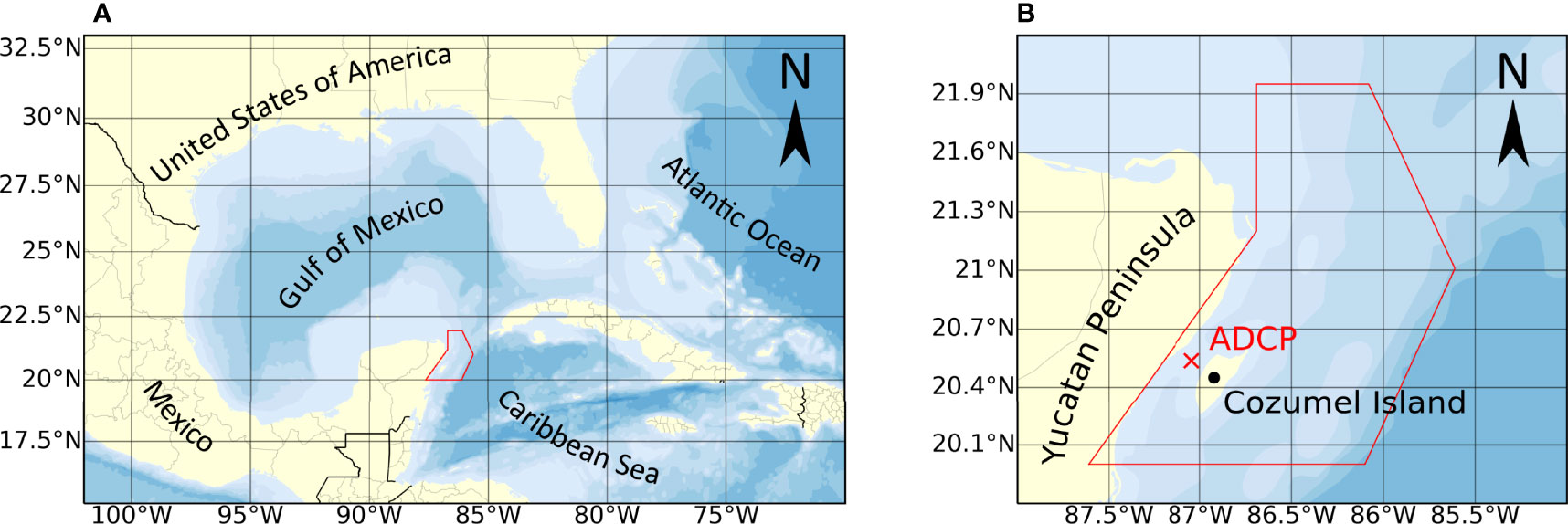
Figure 1 (A) Study area within the Mexican Caribbean and (B) position of the acoustic Doppler current profiler (ADCP).

2 Materials and Methods

2.1 Data Sources

Empirical and numerical data were used for the theoretical analysis presented here. Both sources provide data on the eastward and northward components of the ocean currents in the study area for different depths and different temporal resolutions. The Canek project, which has carried out similar measurements in the past (Chávez et al., 2003), was responsible for the measurements of the current in the Cozumel Channel. The Canek research project, also known as the Estudio de la circulación y elintercambio a través del Canal de Yucatán (Study of circulation and exchange through the Yucatan Canal) has been coordinated by the Centro de Investigación Científica y Educación Superior de Ensenada since its foundation in 1996. The data were obtained using a stationary, long-range acoustic Doppler current profiler at N20°32.218′ W087°02.738′ [see Figure 1B] anchored at a depth of approximately 400m, and measuring every half hour, from 9^th April 2009 to 14^th May 2011. The data on depth were recorded in 16 cells, with the shallowest cell at a depth of 49m. For the numerical data, the HYCOM was chosen because of its good temporal range and resolution, and excellent spatial resolution, compared to other products. In this study, the data of the reanalysis model HYCOM + NCODA GOMu0.04 experiment 50.1 are used, which are publicly available in https://www.hycom.org/data/gomu0pt04/expt-50pt1. The model provides the current components at 40 depths for the Mexican Caribbean (among other regions), covering 1^st January 1993 to 31^st December 2012, at a temporal resolution of three hours and a spatial resolution of 0.04 in both eastern and northern directions. Numerical current data are reported at a depth of 50m while the empirical data describe the current at 49m.

2.2 Validating and Adjusting Numerical Data With Empirical Data

Interpolation of HYCOM data to match the Canek data was carried out using the griddata function, available in the SciPy-module (version 1.6.1) for Python 3 (Virtanen et al., 2020). The four nodes of the numerical model were used as input, which surround the location of the measured field data. Due to the different sampling frequencies of the data sources, the data with higher frequency (i.e., the empirical data) had to be reduced. The data provided by the Canek project were sampled every 30 min and every hour, depending on the date. As the HYCOM numerical data reports the instantaneous value every three-hours, the empirical data were reduced by discarding every time step which is not available in the numerical data.

A linear quantile regression was performed on the current speed, using the quantreg model, as provided by the statsmodels module (version 0.12.2) for Python 3 (Seabold and Perktold, 2010). The linear regression was estimated for the empirical data proportional to the numerical data with the intercept set to zero.

To estimate the error produced by the numerical data, a simplified EVA was performed for both data sets, the empirical data in its original form and the numerical data in its adjusted form but reduced to the temporal range of the empirical data set. The analysis is described in detail in section 2.3. However, due to the low number of observations available in both sets, the methodology had to be modified. As a threshold, the 0.5^th-quantile was used in contrast to the suggested automated threshold selection. However, the same range of possible thresholds was used to estimate the confidence interval. The (signed) relative error between empirical and numerical data is defined as

$\begin{array}{ll}{e}_r = 1 -\frac{u_m}{u_e}, & (1)\end{array}$

where u_e is the empirical current speed and u_m is the speed as predicted by the numerical model. Besides the mentioned modules for Python 3 (Van Rossum and Drake, 2009), substantial parts of the data processing have been carried out with the NumPy-module in version 1.20.1 (Harris et al., 2020) and the pandas-module in version 1.2.2 (Wes McKinney, 2010).

2.3 Extreme Return Levels With Peaks Over Threshold

The methodology used assumes that for a random variable (x) the excess over a suitable threshold (u) can be modelled by a GPD. Liang et al. (2019) define the cumulative density function of the GPD as

$\begin{array}{ll}F\left(x\right)=\{\begin{array}{ll}1-{\left(1+\xi \frac{x-u}{\sigma }\right)}^{(-1\mathrm{/\xi })}\hfill & \text{for}\hspace{0.17em}\xi \ne 0\hfill \\ 1-\text{exp }\left(-\frac{x-u}{\sigma }\right)\hfill & \text{for}\hspace{0.17em}\xi =0\hfill \end{array}\hspace{0.17em}\hspace{0.17em}\hspace{0.17em}\hspace{0.17em},\hspace{0.17em}\hspace{0.17em}\text{with}\hspace{0.17em}x\ge u\hspace{0.17em}\hspace{0.17em}\hspace{0.17em},& (2)\end{array}$

Where x represents the random variable, u the threshold, ξ the shape parameter, and σ the scale parameter.

The procedure can be summarized as follows, where the automated threshold selection method is based on the work of Thompson et al. (2009):

1. Selection of peaks using a moving time window.

2. Detection and filtering of outliers using the quartile method.

3. Identification of potential thresholds between the 25^th and 98^th percentiles, or the 100^th highest peak, whichever is less.

4. For each potential threshold u_j:

(a) Fit a GPD through all peaks for which x_i > u_j.

(b) Determine a reparameterised scale parameter $\left({\sigma }_i^{\ast }\right)$ and its difference $\left(\Delta {\sigma }_i^{\ast }\right)$ tothe next higher threshold (u_j+1).

(c) Fit the normal distribution with zero mean through the difference of the reparameterised scale parameter corresponding to the current and all greater thresholds $\left(\Delta {\sigma }_i^{\ast }|u_i\ge u_j\right)$.

5. Selection of the lowest threshold for which the p-value of the normal distribution through the difference of the reparameterised scale parameter is greater than a significance level of 5%.

6. Estimation of the return levels based on the selected threshold.

To consider the phenomenon as random, the realization of each variable should be independent. However, with the temporal resolution provided, the data analysed in this study is not random. To select only values independent of temporally close values (later called peaks), a moving time window was used, as suggested in Solari et al. (2017). The time window is of fixed length, depending on the variable type, and moves consecutively through the time series. If the value in the centre of the time window is the maximum of that time window, this value is selected as an independent peak.

Outliers may be present in the set of selected peaks, which would alter the final excess model. For the automated and semi-automated detection of outliers, a great variety of methods are available (Hodge and Austin, 2004). One of the simplest methods suitable for univariate data is based on quartiles and presented in Laurikkala et al. (2000). The authors define an upper (u_u) and lower threshold (u_l), beyond which all peaks are considered as outliers and are consequently discarded. Both thresholds are defined by

$\begin{array}{ll}{u}_l=q_1-1.5\left(q_3-q_1\right)& (3)\end{array}$

$\begin{array}{ll}{u}_u=q_3+1.5\left(q_3-q_1\right)\hspace{0.17em}\hspace{0.17em},& (4)\end{array}$

where q₁ is the first quartile (25^th percentile) and q₃ is the third quartile (75^th percentile).

From the previously selected peaks, potential thresholds are selected, as suggested in Thompson et al. (2009). The potential thresholds are equally spaced between 25^th and 98^th percentile. If less than 100 peaks are found above the 98^th percentile, the 100^th largest peak is selected as the upper limit of the range for potential thresholds.

For each threshold, all peaks x_i > u_j are selected, and a GPD is fitted through those peaks. The shape (ξ_j) and scale (σ_j) parameters of the GPD are determined by the function genpareto.fit, which is part of the SciPy.stats-package. The location parameter is held fixed to the corresponding threshold u. The reparameterised scale parameter, which is defined by

$\begin{array}{ll}{\sigma }_j^{\ast }={\sigma }_j-{\xi }_j{u}_j\hspace{0.17em}\hspace{0.17em},& (5)\end{array}$

should be constant above a suitable threshold, following Coles (2001). This relationship was extended by Thompson et al. (2009) by fitting a normal distribution with a mean of zero through the difference of the reparameterised scale parameter for the current and all greater thresholds. This difference is defined by

$\begin{array}{ll}\Delta {\sigma }_j^{\ast }={\sigma }_{j+1}^{\ast }-{\sigma }_j^{\ast }\hspace{0.17em}\hspace{0.17em}.& (6)\end{array}$

The first threshold for which the corresponding normal distribution has a p-value ≥ 0.05 is selected for calculating the return levels. As a test for normality, the Kolmogorov-Smirnov test is used, as implemented in the ks_1samp function of the SciPy.stats-package. The return level X_m (Coles, 2001) can be calculated as

$\begin{array}{ll}{x}_m=\{\begin{array}{ll}u+\frac{\sigma }{\xi }\left({\left(m{\zeta }_u\right)}^{\xi }-1\right)\hfill & \text{for}\hspace{0.17em}\xi \ne 0\hfill \\ u+\sigma \text{log }\left(m{\zeta }_u\right)\hfill & \text{for}\hspace{0.17em}\xi =0\hfill \end{array}\hspace{0.17em}\hspace{0.17em}\hspace{0.17em}\hspace{0.17em}.& (7)\end{array}$

The average number of peaks m during a return period (T_B) is defined by

$\begin{array}{ll}m=\frac{n_p}{n_y}\hspace{0.17em}{T}_B\hspace{0.17em}\hspace{0.17em}\hspace{0.17em},& (8)\end{array}$

where n_p is the total number of peaks and n_y the number of years for which data is available.

The exceedance probability of threshold ${\widehat{\zeta }}_u$, the complete Variance-Covariance Matrix V and the variance of return level $\text{Var}\hspace{0.17em}\left({\widehat{x}}_m\right)$ are estimated, as stated in the following equations (Coles, 2001), where the values with a hat indicate the estimation of the corresponding value.

$\begin{array}{ll}{\widehat{\zeta }}_u=\frac{n_{pot}}{n_p}\hspace{0.17em}\hspace{0.17em}\hspace{0.17em},& (9)\end{array}$

where n_pot is the number of peaks over threshold

$\begin{array}{ll}V=\left[\begin{array}{ccc}\frac{{\widehat{\zeta }}_u}{n_p}\left(1-{\widehat{\zeta }}_u\right)& 0& 0\\ 0& \text{Var }(\widehat{\sigma })& \text{Cov }(\widehat{\sigma },\widehat{\xi })\\ 0& \text{Cov }(\widehat{\xi },\widehat{\sigma })& \text{Var }(\widehat{\xi })\end{array}\right]\hspace{0.17em}\hspace{0.17em}\hspace{0.17em},& (10)\end{array}$

$\begin{array}{ll}\text{Var }({\widehat{x}}_m)=\nabla {\widehat{x}}_m^T\hspace{0.17em}V\hspace{0.17em}\nabla {\widehat{x}}_m\hspace{0.17em}\hspace{0.17em}\hspace{0.17em}\hspace{0.17em}\hspace{0.17em},& (11)\end{array}$

with

$\begin{array}{ll}\nabla {\widehat{x}}_m\begin{array}{c}\begin{array}{l}={\left[\frac{\partial x_m}{\partial {\zeta }_u},\frac{\partial x_m}{\partial \sigma },\frac{\partial x_m}{\partial \xi }\right]}^T\\ =\left[\begin{array}{c}\sigma m^{\xi }{{\zeta }_u}^{\xi -1}\\ {\xi }^{-1}\left({\left(m{\zeta }_u\right)}^{\xi }-1\right)\\ -\sigma {\xi }^{-2}\left({\left(m{\zeta }_u\right)}^{\xi }-1\right)+\sigma {\xi }^{-1}{\left(m{\zeta }_u\right)}^{\xi }\text{log }\left(m{\zeta }_u\right)\end{array}\right]\end{array}\end{array}& (12)\end{array}$

3 Results

3.1 Numerical Data Accuracy

The empirical and numerical data used have different temporal resolutions. Therefore, the empirical data from the Canek project were downsampled by discarding all time steps that are unavailable in the data provided by the numerical model. In Figure 2 the unadjusted numerical data show a clear bias towards overestimation. The numerical data were adjusted by the linear regression model, which was estimated with a quantile regression using the 0.5^th-quantile, and is defined by

$\begin{array}{ll}{u^{\prime }}_m=0.791831u_m\hspace{0.17em}\hspace{0.17em},& (13)\end{array}$

FIGURE 2

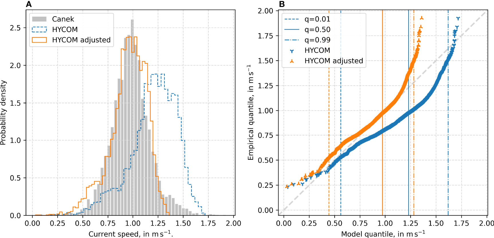
Figure 2 Adjustment of the HYCOM numerical data to the Canek-project empirical data [from the ADCP shown in Figure 1 (B)]. (A) Histogram showing the numerical data before and after the adjustment. (B) Q-Q plot of numerical data before and after the adjustment. The 0.01^st 0.5^th and 0.99^th-quantiles are marked for both data sets.

where u^′_m is the adjusted current speed. The adjusted numerical data reflect the empirical data much better. The effect of the model adjustment is strongly reflected by the mean relative error, that is reduced from −0.255 to 0.006. The mean absolute relative error of 0.288 and the root mean squared relative error of 0.365 are reduced to 0.153 and 0.206, respectively. Of greater concern, however, is the missing tail of the probability distribution of both numerical data in Figurs 2A, as these are of great importance for EVAs. Especially in the adjusted data, this leads to a pronounced underestimation of higher current speeds (i.e., rare events) as seen in the deviation from the diagonal in Figure 2B.

To quantify the effect of the missing tail on the extreme value estimations, a simplified EVA was performed. Due to the short time range, the length of the time window was reduced to 7 days (i.e., 56 observations). Additionally, the 0.5^th-quantile was selected as the threshold rather than the proposed automated threshold selection. As expected from the results presented in Figure 2B, the adjusted numerical model shows an underestimation of extreme values, as can be seen in Figure 3A. Nevertheless, for rare events (return period > 10 years) the relative error converges to a value just below 0.22 (see Figure 3B). The large 95% confidence interval (CI_95%) in Figure 3A is the result of the short temporal coverage of the data used for the analysis. It should be noted that the CI in Figure 3B is not CI_95%; it is the maximum error estimated by the upper and lower bounds of the CI_95% in Figure 3A.

FIGURE 3

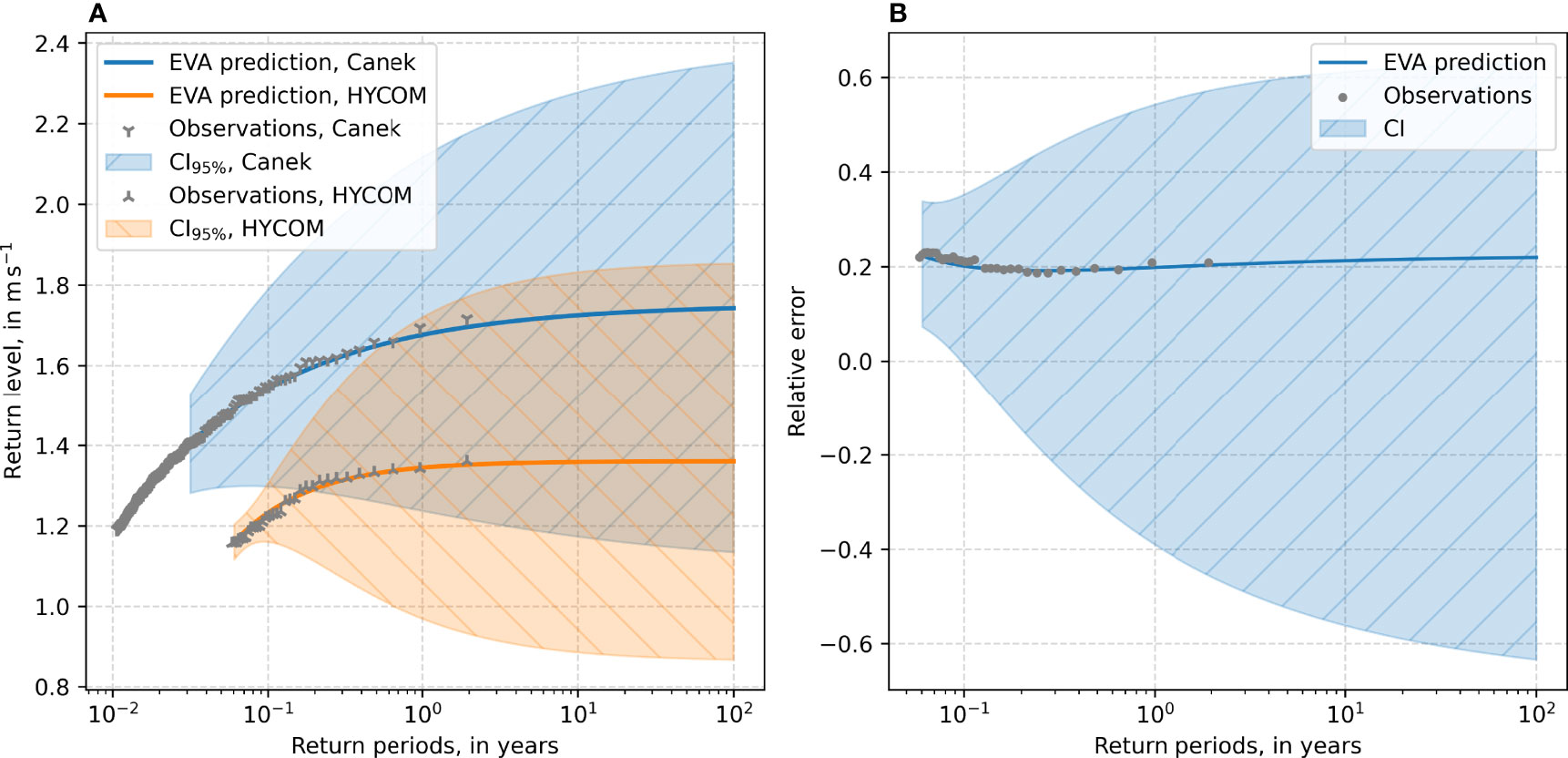
Figure 3 Results of the simplified EVA for the adjusted numerical and empirical data. The adjusted numerical data are limited to the temporal range of the empirical data. (A) Return level plot. (B) Relative error of estimated return levels.

3.2 Extreme Value Analysis

The methodology was applied to several nodes in the Mexican Caribbean, shown as grey dots in Figure 4. It should be noted that not every node contains data on the current, as some are on land, or in waters of less than 50m depth. The four nodes marked in red were selected as the results suggest that it is possible to obtain a different behaviour with respect to the GPD fit. The node at position P1 (20.520° N, 86.600° W) is where the current is most concentrated off the east coast of Cozumel. The node at position P2 (20.640° N, 86.960° W), is in the Cozumel Channel, near a possible site for the installation of ocean current turbines [see Alcérreca-Huerta et al. (2019)]. That at P3 (21.040° N, 86.560° W) is in the wake of the Cozumel Channel, off the coast of Cancun, and the node at P4 (21.800° N, 86.480° W) is in the Yucatan current northeast of Cancun.

FIGURE 4

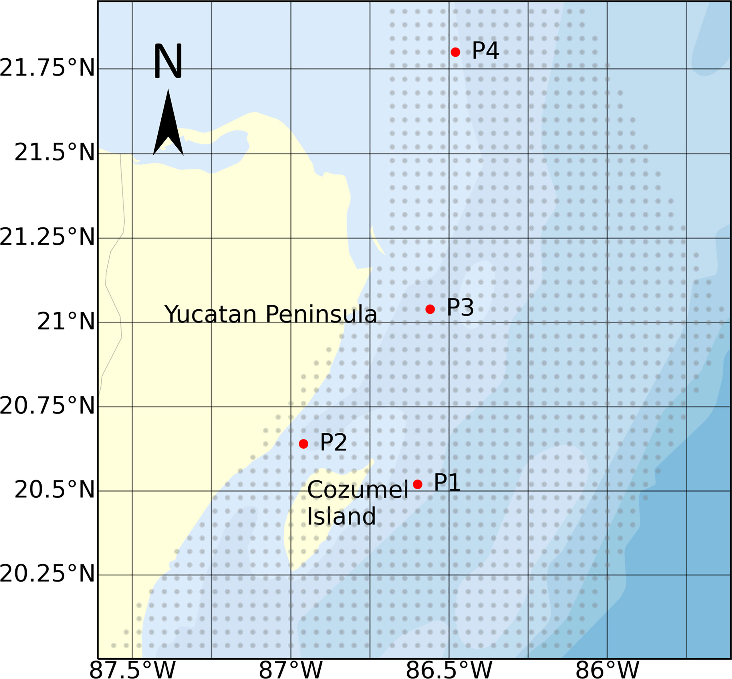
Figure 4 Location of the nodes for the numerical model which lie within the study area. The nodes marked in red are positions for which more details regarding the GPD fit are presented.

To determine the optimal length of the time window, the number of peaks identified in the windows was analysed for the nodes at P1 to P4. In Figure 5A, there is a steady fall in the number of peaks, but it remains above the critical number of 200. At a length of 25 days, the number of peaks for all four nodes is just below 250. The relative difference between the number of peaks and the length of time window (see Figure 5B) shows a decreasing trend, as the length of the time window increases. From a 21 day length, the relative difference is less than 10%, dipping briefly below the 5% mark at a length of 23 days. To spread the number of peaks evenly within the time range analysed, and to avoid having too few peaks, a time window of 23 days in length was chosen.

FIGURE 5

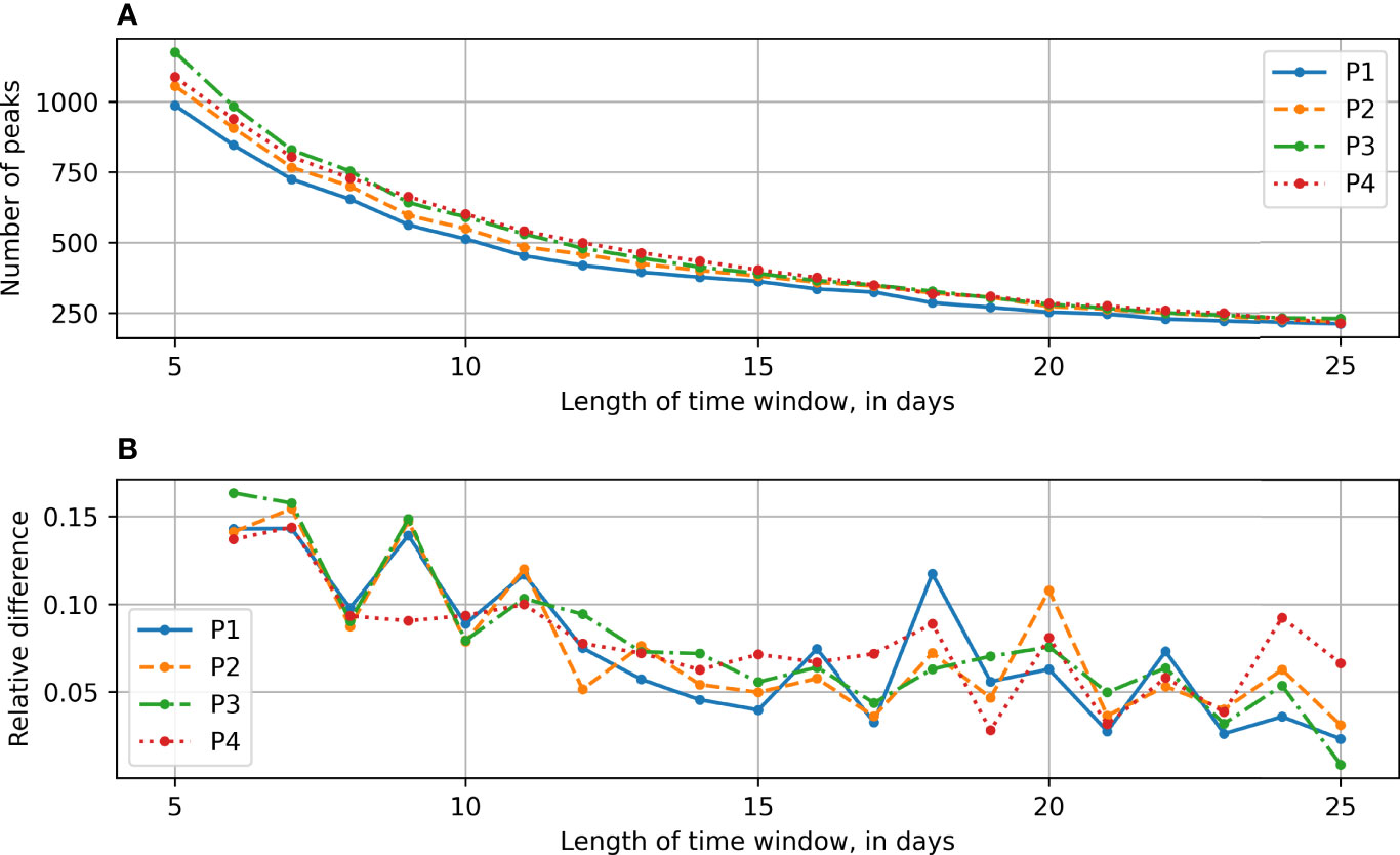
Figure 5 Relation between the number of independent peaks and the length of the time window for the nodes at P1 to P4. (A) Number of identified peaks. (B) Relative difference in number of identified peaks to previous time window length.

Figure 6 shows the statistical data of the GPD fit for each node. While the north, east, and southern boundaries of the domain are determined by the node selection, the western boundary is a feature of the numerical data generated by HYCOM for this site. The number of identified peaks seems to be similar in the study region (see Figure 6A), with a slight decrease towards deeper waters.

FIGURE 6

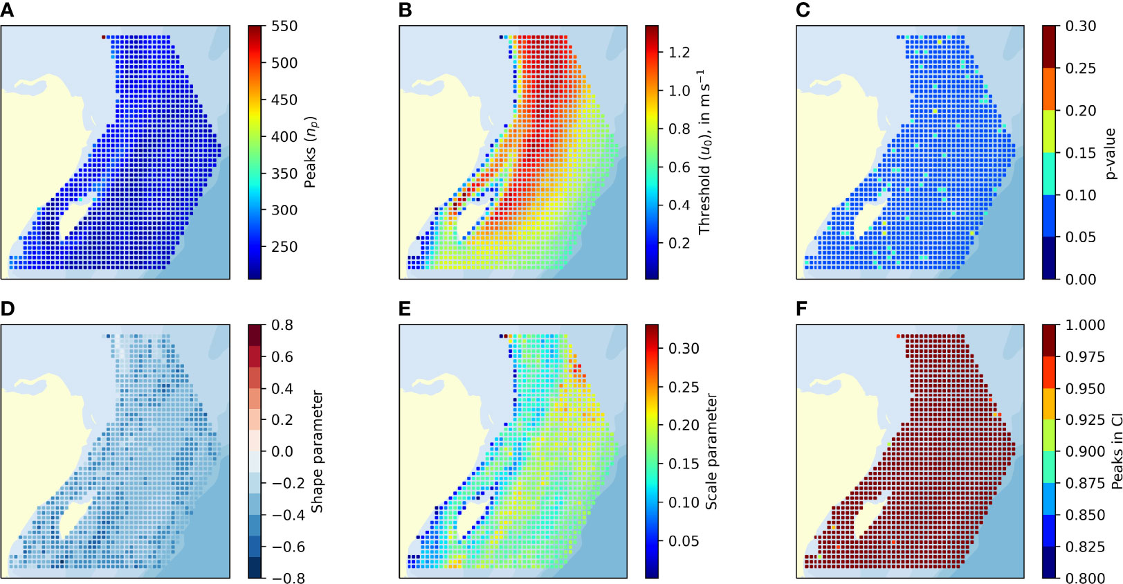
Figure 6 Statistical data for the GPD fit. (A) Number of identified peaks. (B) Selected thresholds. (C) p-value for the selected thresholds. (D) Shape factor for GPD fit to POT. (E) Scale factor for GPD fit to POT. (F) Share of peaks within the CI_95%.

Figures 6B, C) show the selected threshold for each node and the corresponding p-value for the automatic threshold selection, respectively. The value of selected thresholds tend to increase in the centre of the channel, and in the stream close to the east coast of Cozumel Island that extends northward, along the Cancun coast. This is expected, since the current becomes more intense at these locations. As it was possible to find a suitable threshold for all nodes with information on the current velocity, the p-value is over 0.05 in significance, although some inconsistencies of above 0.1, and even 0.15, are found throughout the domain.

There is no clear trend in the shape parameter of the fitted GPD in Figure 6D. However, it was estimated to be negative for all nodes, producing a bounded GPD. For a few nodes at the northwestern boundary, the shape parameter was estimated to be very close to zero. The scale parameter in Figure 6E indicates a slight increase off Cozumel Island and at the northeastern boundary, which leads to a thicker tail for the GPD in those regions (i.e., increased return levels).

Figure 6F shows the number of peaks above the threshold which lie within the estimated CI_95%. For nearly all the nodes, the estimated CI_95% covers 100% of the numerical observations. As is to be expected, not all the observations are within the CI_95% for all the nodes. However, the number of nodes for which some observations are outside the CI_95% is small, while the minimum share within the analysed region is still above 90%. Despite this apparent overestimation of the CI_95%, this suggests that the methodology of GPD fit together with the estimation of the CI_95% is suitable and the results of the GPD for the given input data is reliable.

Return levels for the selected return periods, on the corresponding lower and upper boundaries of the CI_95% are shown in Figure 7. The expected return level (central column) increases in the channel and the main current, which extends northwards from the east of the Cozumel Island. This trend is further pronounced in the case of the CI_95% upper boundary (right column of Figure 7), which is in agreement with the results in Figures 6B, E. The region with higher shape parameters at the northwest edge of the domain (see Figure 6D) is not noticeable in the estimated return level (centre column in Figure 7). However, in case of the CI95%-limits, that region stands out with lower return level for the lower bound of the CI_95% and higher return levels for the upper limit, suggesting a much higher uncertainty. The distribution over the rest of the domain is as expected, see Figure 6.

FIGURE 7

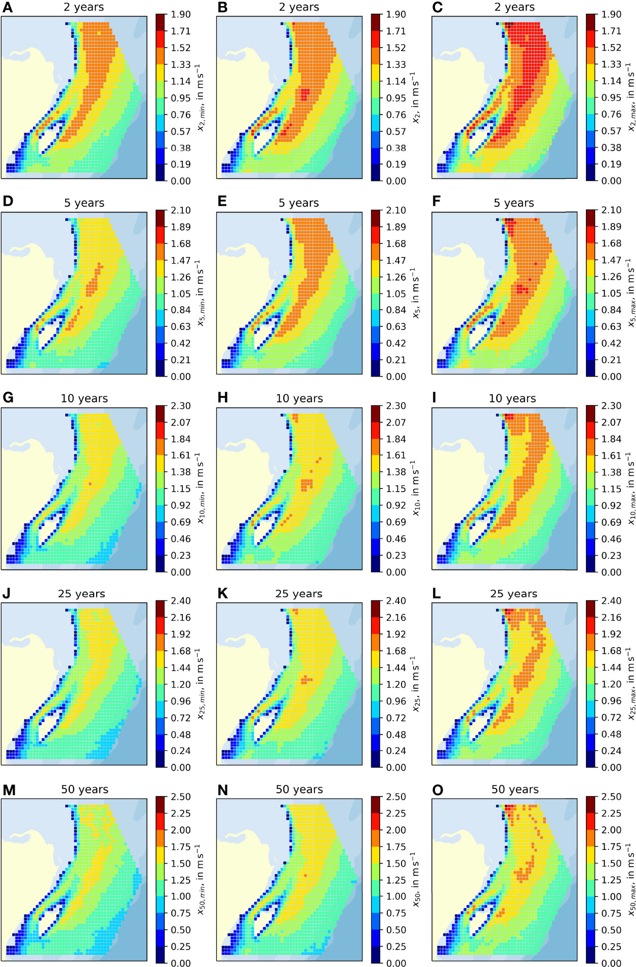
Figure 7 Return levels for 50m depth for different return periods. All the figures in one row correspond to the same return period; (A–C) 2 years, (D–F) 5 years, (G–I) 10 years, (J–L) 25 years, and (M–O) 50 years. The left column shows the lower bound of the CI_95%, the right column the upper bound of the CI_95%, and the central column the predicted return level.

The parameters for the GPD excess model for the four nodes seen in Figure 4 are summarized in Table 1. Except for the node at position P4, the shape parameters are negative, with all of CI_95% below zero. Compared to the standard error, the shape parameter at P4 is small, giving a CI_95% closely centred around zero. However, this result could be due to an error in the numerical model, as mentioned above. The highest scale parameter is found at P1, which produces a thicker tail to the probability distribution. Nevertheless, the bound nature of the excess model (due to the negative shape parameter) prevents high return levels for this node. The number of peaks found for each node is similar, just above the critical threshold of 200. Slightly more than 100 peaks were found above the selected threshold. The number of peaks, and peaks above the threshold, suggests that the selected time span of 20 years is a bit short, but still sufficient to perform the EVA.

TABLE 1

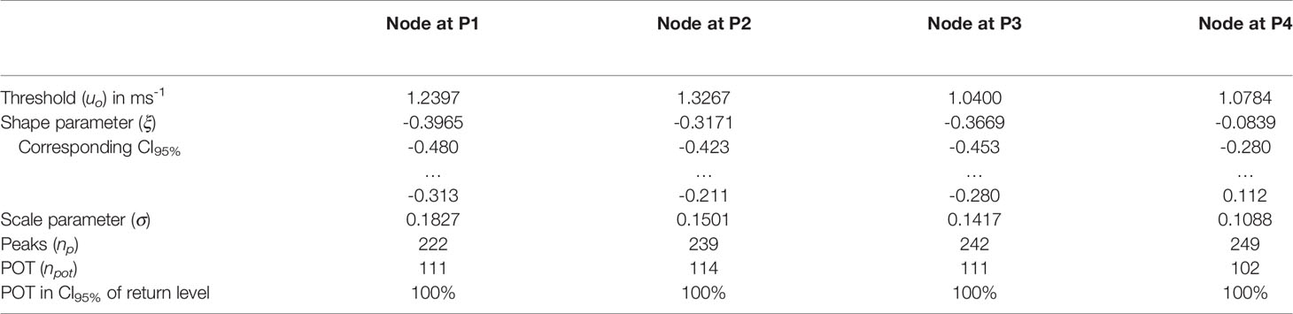
Table 1 Values for GPD fit for four nodes.

In Figure 8, the peaks, POT, and the thresholds are shown for the four nodes. None of these nodes have a cluster of peaks (or lack thereof), suggesting that a 23 day time window is sufficient. The distributions of peaks, together with the filtered outliers, are shown for each node in Figure 9. The nodes at P1 to P3 show a standard distribution of peaks. The node at P4 has a multi-modal distribution, suggesting an error, and that the conclusions drawn from the data might not be reliable. No outliers at the upper end were found for the node at P2, whereas at P1 and P4 there were one each, and at P3, two. At the lower end, a few outliers were also detected and filtered out, but due to the nature of POT methods, these tend to have no significant effect on the outcome.

FIGURE 8

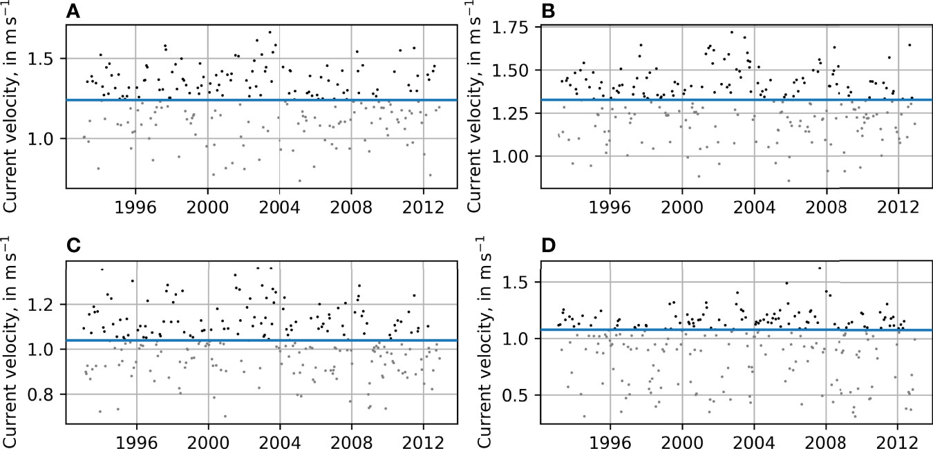
Figure 8 Distribution of peaks over time for the nodes at P1 to P4, as identified by means of a 23 days moving time window. The peaks under threshold are marked with grey dots, the peaks over threshold with black dots, and the selected threshold by the blue line. (A) Node at P1, (B) Node at P2, (C) Node at P3, and (D) Node at P4.

FIGURE 9

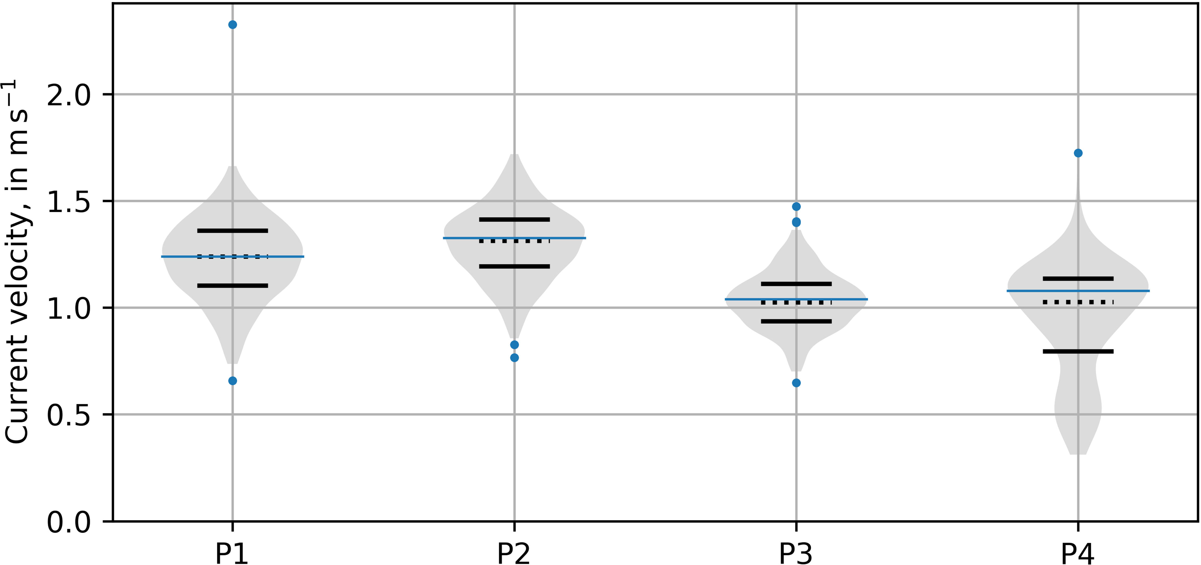
Figure 9 Detected outliers and distribution of peaks for nodes at P1 to P4. The first and third quartiles are shown as solid lines and the median as a dotted line. The filtered outliers are shown as blue dots and the selected threshold as a thin blue line.

Figures 10–13 present the corresponding diagnostic plots for the GPD excess model. For a detailed interpretation of this type of plot, the reader is referred to Coles (2001). Despite slight deviations in the diagnostic plot for the node at P1 in Figure 10, and especially the q-q plot in Figure 10B, 100% of the empirical POT still lie within the CI_95%, as seen in Figure 10C and tab. 1. Both plots suggest an overestimation of the GPD model. There are few peaks, especially visible in the density plot (Figure 10D). However, the bound excess model seems to give a good fit for the underlying numerical data. The diagnostic plots for the node at P2 (Figure 11) show some deviations between the numerical data and GPD excess model in the p-p plot (Figure 11A). Around the 0.6 mark, the GPD excess model shows a slight overestimation. This deviation is also visible in the q-q plot (Figure 11B) at speeds of about 1.45ms−1 and in the return level-plot (Figure 11C) at the same speeds. Despite these inconsistencies, the GPD excess model is a fits the data well.

FIGURE 10

Figure 10 Diagnostic plot for the GPD excess model fitted to 3-hourly current for the node at P1. (A) p-p plot, (B) q-q plot, (C) return level plot, and (D) density plot.

FIGURE 11

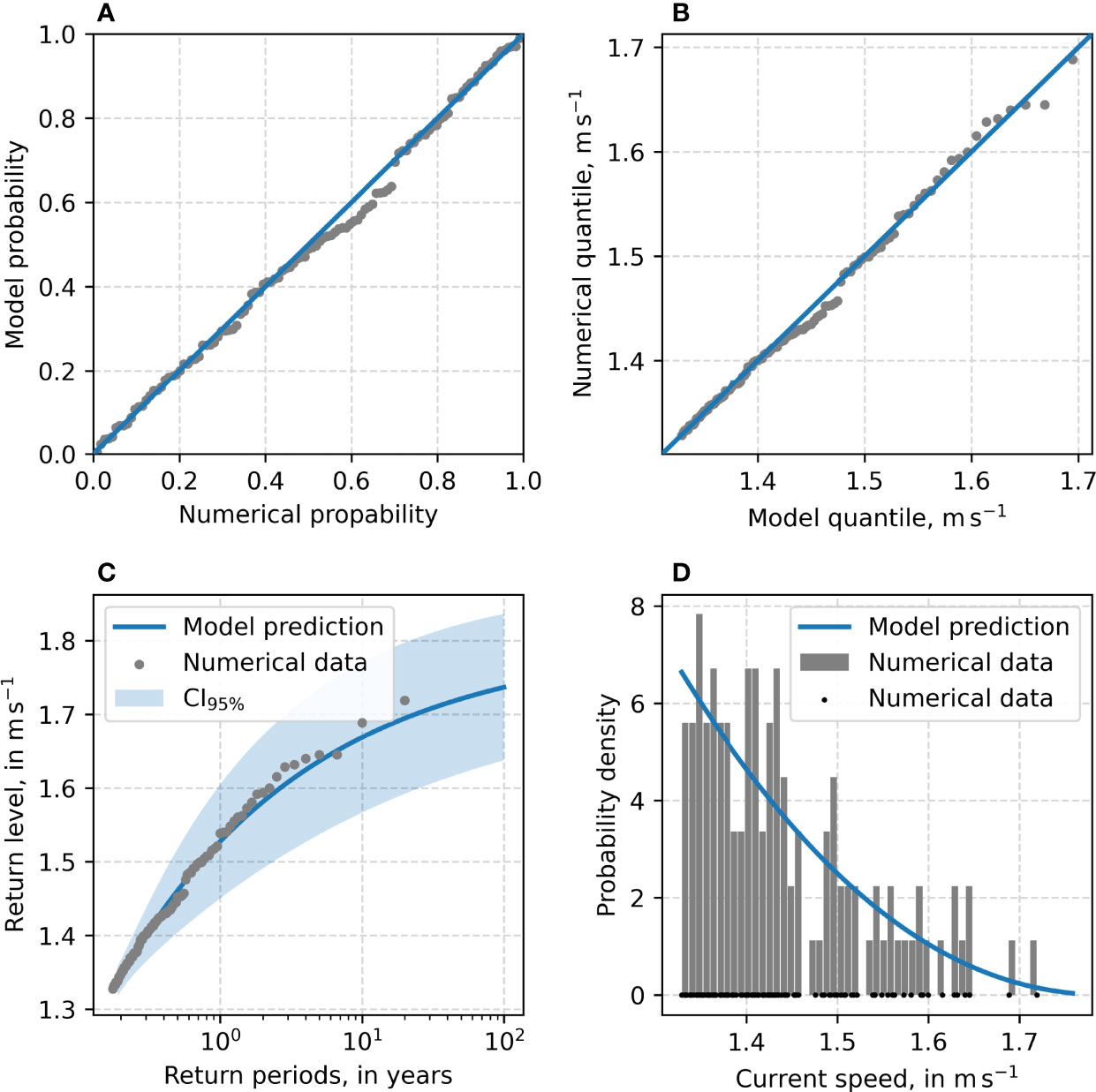
Figure 11 Diagnostic plot for the GPD excess model fitted to 3-hourly current for the node at P2. (A) p-p plot, (B) q-q plot, (C) return level plot, and (D) density plot.

The p-p plot presents some discrepancies at the 60% percentile at P3 (Figure 12A). The excess model also differs from the numerical data for higher speeds, as seen in Figures 12B, C. However, all the observations are within the estimated CI_95% of the return level, suggesting that the GPD excess model application is reliable.

FIGURE 12

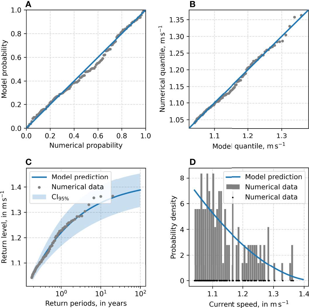
Figure 12 Diagnostic plot for the GPD excess model fitted to 3-hourly current for the node at P3. (A) p-p plot, (B) q-q plot, (C) return level plot, and (D) density plot.

The plots in Figure 13 bring into doubt whether this excess model can be used to reliably estimate the extreme values of the node at P4. Although the CI_95% includes all the numerical observations, the p-p plot (Figure 13A) and especially the q-q plot (Figure 13B) looks unusual. A slight s-shaped deviation is present, with considerable inconsistencies above 1.2ms⁻¹ in the q-q plot. Additionally, and as observed in Figure 7, the CI_95% in Figure 13C is quite large, while the density plot in Figure 13D shows a reasonable fit to the data.

FIGURE 13

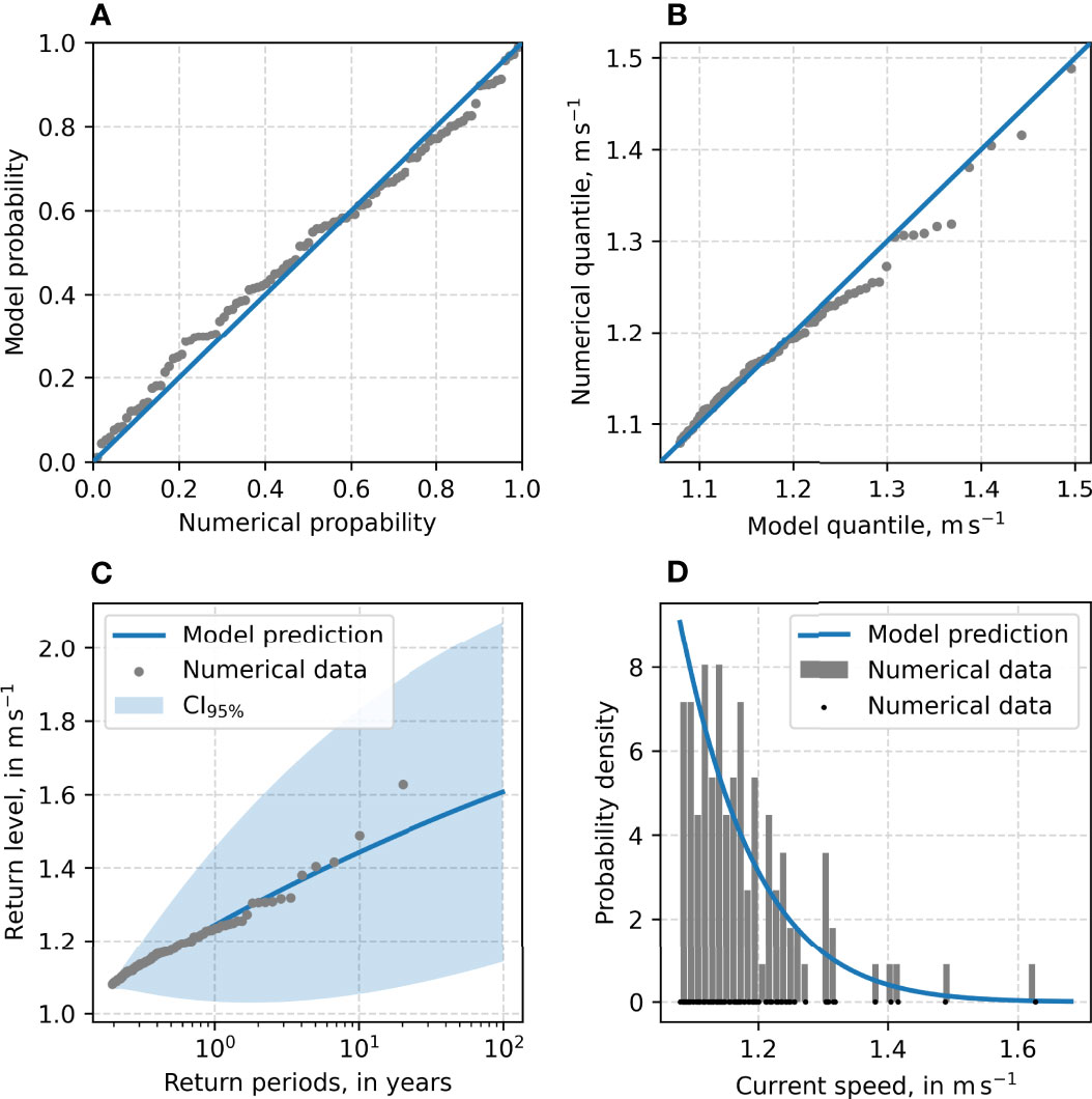
Figure 13 Diagnostic plot for the GPD excess model fitted to 3-hourly current for the node at P4. (A) p-p plot, (B) q-q plot, (C) return level plot, and (D) density plot.

4 Discussion

For adjustment of the numerical data, the empirical and numerical data were filtered to match their time steps. The high relative error of -25.5% was reduced to 0.6% by linear quantile regression. However, the mean absolute relative error and the root mean square relative error cannot be reduced in the same way. This indicates that, despite the adjustment, the numerical model is not able to accurately reproduce the behaviour of the current in this region. Furthermore, the lack of the tail in the numerical data histogram proves that there is still room to improve the HYCOM numerical model. The effect of the missing tail on extreme value predictions was estimated with a simplified EVA. Despite the short time series, the error can be estimated at 22% underestimation for rare events with a return period of > 10years. However, the error presents very low variability for rare events, and the error converges to a value close to 22%. This makes it easy to account for in design processes. Nevertheless, these results should be addressed in future research in order to accurately identify the source of the error and to characterize it over a larger area, instead of a single point.

As shown by the large CI_95% of the simplified EVA, the temporal coverage of the empirical data is not sufficient to reliably estimate extreme values. However, the error between the extreme value predictions of empirical and numerical data is consistent. This error gives the necessary information to have sufficiently detailed knowledge on the extreme value predictions derived from the HYCOM model.

For most of the nodes, the EVA showed consistent behaviour over the domain analysed. Some inconsistencies were found, especially at the boundary of the numerical domain and on the northwest edge of the continental shelf. Besides the significant changes in the bathymetry in those regions, the ordered grid of the numerical model might not be fully capable of representing the nature of the current in boundaries that are not aligned with the grid. As can be seen for the node at P4, the estimated CI_95% is large, and the multimodal peak distribution suggests an unusual behaviour of the HYCOM data for this area. The results for these nodes may be unreliable, and it is suggested that the data obtained for these locations is used with special care.

The other three nodes, which had more information on the GPD fit, showed unremarkable results, as the EVA represents a good fit for the numerical observations. For most nodes, 100% of the numerical observations were found to be within the estimated CI_95%. This share should be much closer to 95%, indicating that the estimated CI_95% is larger than it should be. In contrast to the assumed symmetric distribution of the CI_95%, a log-likelihood profile could give better results and might be investigated in future studies if the overestimation of the CI_95% represents an issue.

The extreme values found a reasonable distance from the coast vary considerably. Therefore, it is important to carefully select a region with similar behaviour in terms of GPD fit. Basing design values on a region with heterogeneous behaviour could lead to erroneous design choices. Besides the variability, regions with similar return periods are found on either side of Cozumel Island. In terms of extreme currents, with reduced effort it may be possible to adapt energy harvesting devices designed for Cozumel Channel conditions to the conditions on the east coast of Cozumel.

5 Conclusions

It was found that the HYCOM model does not accurately reproduce the current velocities in the Cozumel Channel. Adjusting the model with a linear quantile regression reduces the mean absolute relative error to 15.3%, but the lack of a tail in the distribution of the numerical data leads to an underestimation of extreme values of almost 22%.

Applied to a range of nodes within the Mexican Caribbean, the methodology showed consistently – and to some extent predictable – behaviour. In the Cozumel Channel and in the main current, the threshold and the extreme values are naturally higher than in regions with lower current intensities. The difference in return levels can be explained by the threshold and the scale parameter.

Despite the shortcomings of the numerical model, the methodology presented for estimating extreme values of ocean currents based on HYCOM data proves to be a valuable tool due to the predictability of the error for extreme values.

Data Availability Statement

The raw data supporting the conclusions of this article are available from the corresponding author, MR, upon reasonable request.

Author Contributions

Conceptualization and methodology: PR-O and MR; data processing, analysis and visualisation: MR; writing – original draft preparation: PR-O and MR; writing – review and editing: PR-O, MR, RS, and EM; supervision and project administration: RS and EM; funding acquisition: EM; All authors contributed to manuscript revision, read, and approved the submitted version.

Funding

This research was funded by the CONACYT-SENER-SUSTENTABILIDAD ENERGÉTICA project: FSE-2014-06-249795 “Centro Mexicano de Innovación en Energía del Océano (CEMIE Océano)”.

Conflict of Interest

The authors declare that the research was conducted in the absence of any commercial or financial relationships that could be construed as a potential conflict of interest.

Publisher’s Note

All claims expressed in this article are solely those of the authors and do not necessarily represent those of their affiliated organizations, or those of the publisher, the editors and the reviewers. Any product that may be evaluated in this article, or claim that may be made by its manufacturer, is not guaranteed or endorsed by the publisher.

Acknowledgments

The authors would like to thank Julio Candela and Julio Sheinbaum for permission to use their empirical data and Jill Taylor for reviewing the English language. Furthermore, the first author is grateful for the financial support provided by the CONACYT doctoral fellowship.

Abbreviations

GPD, Generalized Pareto Distribution; HYCOM, Hybrid Coordinate Ocean Model; POT, Peaks over threshold; CI_95%, 95% confidence interval.

References

Abascal A. J., Sheinbaum J., Candela J., Ochoa J., Badan A. (2003). Analysis of Flow Variability in the Yucatan Channel. J. Geophys. Res. C.: Ocean. 108, 11–11. doi: 10.1029/2003JC001922

CrossRef Full Text | Google Scholar

Alcérreca-Huerta J. C., Encarnacion J. I., Ordoñez-Sánchez S., Callejas-Jiménez M., Barroso G. G. D., Allmark M., et al. (2019). Energy Yield Assessment From Ocean Currents in the Insular Shelf of Cozumel Island. J. Mar. Sci. Eng. 7, 1–18. doi: 10.3390/jmse7050147

CrossRef Full Text | Google Scholar

Athie G., Candela J., Sheinbaum J., Badan A., Ochoa J. L. (2011). Yucatan Current Variability Through the Cozumel and Yucatan Channels. Cienc. Mar. 37, 471–492. doi: 10.7773/cm.v37i4a.1794

CrossRef Full Text | Google Scholar

Bárcenas Graniel J. F., Fontes J. V. H., Garcia H. F. G., Silva R. (2021). Assessing Hydrokinetic Energy in the Mexican Caribbean: A Case Study in the Cozumel Channel. Energies 14, 4411. doi: 10.3390/en14154411

CrossRef Full Text | Google Scholar

Bore P. T., Amdahl J., Kristiansen D. (2019). Statistical Modelling of Extreme Ocean Current Velocity Profiles. Ocean. Eng. 186, 106055. doi: 10.1016/j.oceaneng.2019.05.037

CrossRef Full Text | Google Scholar

Carrillo González F., Ochoa J., Candela J., Badan A., Sheinbaum J., González Navarro J. I. (2007). Tidal Currents in the Yucatan Channel. Geofis. Internacional. 46, 199–209. doi: 10.22201/igeof.00167169p.2007.46.3.39

CrossRef Full Text | Google Scholar

Cetina P., Candela J., Sheinbaum J., Ochoa J., Badan A. (2006). Circulation Along the Mexican Caribbean Coast. J. Geophys. Res.: Ocean. 111, 1–19. doi: 10.1029/2005JC003056

CrossRef Full Text | Google Scholar

Chávez G., Candela J., Ochoa J. (2003). Subinertial Flows and Transports in Cozumel Channel. J. Geophys. Res. C.: Ocean. 108, 19–11. doi: 10.1029/2002JC001456

CrossRef Full Text | Google Scholar

Coles S. (2001). “An Introduction to Statistical Modeling of Extreme Values”, in Springer Series in Statistics (London, UK: Springer-Verlag).

Google Scholar

Coles S., Simiu E. (2003). Estimating Uncertainty in the Extreme Value Analysis of Data Generated by a Hurricane Simulation Model. J. Eng. Mechanics. 129, 1288–1294. doi: 10.1061/(asce)0733-9399(2003)129:11(1288

CrossRef Full Text | Google Scholar

Devis-Morales A., Montoya-Sánchez R. A., Bernal G., Osorio A. F. (2017). Assessment of Extreme Wind and Waves in the Colombian Caribbean Sea for Offshore Applications. Appl. Ocean. Res. 69, 10–26. doi: 10.1016/j.apor.2017.09.012

CrossRef Full Text | Google Scholar

Fan S., Dupuis K., Harrington-Missin L., Calverley M., Watson A., Jeans G. (2010). Validation of HYCOM Current Profiles Using MMS NTL Observations. Proc. Annu. Offshore. Technol. Conf. 3, 2135–2147. doi: 10.2523/20797-ms

CrossRef Full Text | Google Scholar

Harris C. R., Millman K. J., van der Walt S. J., Gommers R., Virtanen P., Cournapeau D., et al. (2020). Array Programming With NumPy. Nature 585, 357–362. doi: 10.1038/s41586-020-2649-2

PubMed Abstract | CrossRef Full Text | Google Scholar

Hernández-Fontes J. V., Felix A., Mendoza E., Cueto Y. R., Silva R. (2019). On the Marine Energy Resources of Mexico. J. Mar. Sci. Eng. 7. doi: 10.3390/jmse7060191

CrossRef Full Text | Google Scholar

Hodge V. J., Austin J. (2004). A Survey of Outlier Detection Methodologies. Artif. Intell. Rev. 22, 85–126. doi: 10.1023/B:AIRE.0000045502.10941.a9

CrossRef Full Text | Google Scholar

Jonathan P., Ewans K. (2013). Statistical Modelling of Extreme Ocean Environments for Marine Design: A Review. Ocean. Eng. 62, 91–109. doi: 10.1016/j.oceaneng.2013.01.004

CrossRef Full Text | Google Scholar

Laurikkala J., Juhola M., Kentala E. (2000). Informal Identification of Outliers in Medical Data. In. 5th. Int. Workshop. Intell. Data Med. Pharmacol. 1, 20–24.

Google Scholar

Liang B., Shao Z., Li H., Shao M., Lee D. (2019). An Automated Threshold Selection Method Based on the Characteristic of Extrapolated Significant Wave Heights. Coast. Eng. 144, 22–32. doi: 10.1016/j.coastaleng.2018.12.001

CrossRef Full Text | Google Scholar

Liu M., Wu W., Tang D., Ma H., Naess A. (2018). Current Profile Analysis and Extreme Value Prediction in the LH11-1 Oil Field of the South China Sea Based on Prototype Monitoring. Ocean. Eng. 153, 60–70. doi: 10.1016/j.oceaneng.2018.01.064

CrossRef Full Text | Google Scholar

Moeini M. H., Etemad-Shahidi A., Chegini V. (2010). Wave Modeling and Extreme Value Analysis Off the Northern Coast of the Persian Gulf. Appl. Ocean. Res. 32, 209–218. doi: 10.1016/j.apor.2009.10.005

CrossRef Full Text | Google Scholar

Morton I. D., Bowers J. (1996). Extreme Value Analysis in a Multivariate Offshore Environment. Appl. Ocean. Res. 18, 303–317. doi: 10.1016/S0141-1187(97)00007-2

CrossRef Full Text | Google Scholar

Niroomandi A., Ma G., Ye X., Lou S., Xue P. (2018). Extreme Value Analysis of Wave Climate in Chesapeake Bay. Ocean. Eng. 159, 22–36. doi: 10.1016/j.oceaneng.2018.03.094

CrossRef Full Text | Google Scholar

Ochoa J., Candela J., Badan A., Sheinbaum J. (2005). Ageostrophic Fluctuations in Cozumel Channel. J. Geophys. Res. C.: Ocean. 110, 1–16. doi: 10.1029/2004JC002408

CrossRef Full Text | Google Scholar

Oliver E. C., Sheng J., Thompson K. R., Blanco J. R. (2012). Extreme Surface and Near-Bottom Currents in the Northwest Atlantic. Nat. Haz. 64, 1425–1446. doi: 10.1007/s11069-012-0303-5

CrossRef Full Text | Google Scholar

Orbital Marine Power Ltd. (2021). Orbital Marine Power Launches O2: World’s Most Powerful Tidal Turbine. Available at: https://orbitalmarine.com/orbital-marine-power-launches-o2 (Accessed date November 16, 2021).

Google Scholar

Park S. B., Shin S. Y., Shin D. G., Jung K. H., Choi Y. H., Lee J., et al. (2020). Extreme Value Analysis of Metocean Data for Barents Sea. J. Ocean. Eng. Technol. 34, 26–36. doi: 10.26748/ksoe.2019.094

CrossRef Full Text | Google Scholar

Qi Y., Shi P. (2009). Calculation of the Extreme Wind, Wave And Current In Deep Water of the South China Sea. The Proceedings of The Third (2009) ISOPE International DEEP-OCEAN TECHNOLOGY SYMPOSIUM: Deepwater Challenge (IDOT-2009)1–7. Available at: http://publications.isope.org/proceedings/ISOPE_IDOT/ISOPE_IDOT_2009/start.htm.

Google Scholar

Robinson M. E., Tawn J. A. (1997). Statistics for Extreme Sea Currents. J. R. Stat. Soc. Ser. C.: Appl. Stat 46, 183–205. doi: 10.1111/1467-9876.00059

CrossRef Full Text | Google Scholar

Seabold S., Perktold J. (2010). “Statsmodels: Econometric and Statistical Modeling With Python”, in In 9th Python in Science Conference 57, 61. doi: 10.25080/Majora-92bf1922-011.

CrossRef Full Text | Google Scholar

Simiu E. (2011). Design of Buildings for Wind: A Guide for ASCE 7-10 Standard Users and Designers of Special Structures: Second Edition (Hoboken, New Jersey, USA :John Wiley and Sons).

Google Scholar

Solari S., Egüen M., Polo M. J., Losada M. A. (2017). Peaks Over Threshold (POT): A Methodology for Automatic Threshold Estimation Using Goodness of Fit P-Value. Water Resour. Res. 53, 2833–2849. doi: 10.1002/2016WR019426

CrossRef Full Text | Google Scholar

Sustainable Marine. (2021). Sustainable Marine Unveils ‘Next-Gen Platform’ Ahead of World-Leading Tidal Energy Project. Available at: https://www.sustainablemarine.com/press-releases/-sustainable-marine-unveils-%E2%80%98next-gen-platform%E2%80%99-ahead-of-world-leading-tidal-energy-project (Accessed date November 16, 2021).

Google Scholar

Thompson P., Cai Y., Reeve D., Stander J. (2009). Automated Threshold Selection Methods for Extreme Wave Analysis. Coast. Eng. 56, 1013–1021. doi: 10.1016/j.coastaleng.2009.06.003

CrossRef Full Text | Google Scholar

Van Rossum G., Drake F. L. (2009). Python 3 Reference Manual (Scotts Valley, CA: CreateSpace).

Google Scholar

Virtanen P., Gommers R., Oliphant T. E., Haberland M., Reddy T., Cournapeau D., et al. (2020). {SciPy} 1.0: Fundamental Algorithms for Scientific Computing in Python. Nat. Methods 17, 261–272. doi: 10.1038/s41592-019-0686-2

PubMed Abstract | CrossRef Full Text | Google Scholar

Viselli A. M., Forristall G. Z., Pearce B. R., Dagher H. J. (2015). Estimation of Extreme Wave and Wind Design Parameters for Offshore Wind Turbines in the Gulf of Maine Using a POT Method. Ocean. Eng. 104, 649–658. doi: 10.1016/j.oceaneng.2015.04.086

CrossRef Full Text | Google Scholar

Wes M. K. (2010). Data Structures for Statistical Computing in Python (Accessed Proceedings of the 9th Python in Science Conference).

Google Scholar