 Haixing Wang1,2
 Donglai Gong1*
 Marjorie A. M. Friedrichs1
 Courtney K. Harris1
 Travis Miles3
 Hao-Cheng Yu1
 Yinglong Zhang1
- 1Virginia Institute of Marine Science, William & Mary, Gloucester Point, VA, United States
- 2Berkshire Hathaway Specialty Insurance, Boston, MA, United States
- 3Department of Marine and Coastal Sciences, Rutgers University, New Brunswick, NJ, United States
Submarine canyons provide a conduit for shelf-slope exchange via topographically induced processes such as upwelling and downwelling. These processes in the Wilmington Canyon, located along the shelf-break of the Mid-Atlantic Bight (MAB), have not been previously studied, and the associated hydrographic variability inside the canyon and on the adjacent shelf are largely unknown. Observations from an underwater glider deployed in Wilmington Canyon (February 27 - March 8, 2016), along with wind and satellite altimetry data, showed evidence for a wind-driven canyon upwelling event followed by a subsequent downwelling event. Next, a numerical model of the MAB was developed to more fully represent these two events. Modeled results showed that under upwelling-favorable winds during February 25 - March 3, sea level increased seaward, shelf currents flowed northeastward, and canyon upwelling developed. Then under downwelling-favorable winds during March 4-7, sea level increased landward, shelf currents flowed southwestward, and canyon downwelling developed. Modeling experiments showed that canyon upwelling and downwelling were sub-tidal processes driven by winds and pressure gradients (associated with SSH gradients), and they would occur with or without tidal forcing. During the upwelling period, slope water originating from 150-215 m depths within the canyon (75 m below the canyon rim), was advected onto the shelf, forming a cold and dense canyon-upwelled slope-originated overflow water at the bottom of the outer shelf (75-150 m isobaths). The dense overflow current flowed was directed northeastward and expanded in the cross-shelf direction. It was 5-20 km wide and 10-30 m thick. The estimated volume of the plume overflow water exceeded 6×10⁹ m3 at peak. The density front at the shoreward side of the dense overflow water caused a subsurface baroclinic frontal jet, which flowed northeastward and along-shelf with maximum speed exceeding 0.5 m/s. In the ensuing downwelling event, a portion of the previously upwelled dense water was advected back to the canyon, and then flowed down-slope in the upper canyon in ~0.3 m/s bottom-intensified currents. Dynamical investigation of the overflow current showed that its evolution was governed by unbalanced horizontal pressure gradient force in the cross-shelf direction and that the current was geostrophic.
1 Introduction
Shelf-break submarine canyons are common geomorphological features that incise the shelf-break, and they provide a conduit for shelf-slope exchange via topographically induced processes such as canyon upwelling and downwelling (Allen and Durrieu de Madron, 2009). Under similar upwelling- or downwelling-favorable conditions, the cross-isobath exchange flow in a canyon is stronger than that over a normal shelf-break (Klinck, 1996; She and Klinck, 2000; Kämpf, 2006). Thus, submarine canyons can drive enhanced shelf-slope exchanges of water masses (Kämpf, 2010; Connolly and Hickey, 2014). Canyon upwelling and downwelling occurs on the sub-inertial time scales and is associated with favorable conditions of along-shelf flows, which is driven by cross-shelf sea surface height gradients and winds. For canyons in the northern hemisphere, upwelling occurs under left-bounded along-shelf flows (flows with the coast to their left side; Klinck, 1996). Canyon upwelling and left-bounded along-shelf flows are often associated with seaward cross-shelf sea surface height gradients (∇SSH) that produce sea-level set-down at the coast (Freeland, 1982; Allen and Hickey, 2010), which in turn are often forced by upwelling-favorable winds (left-bounded along-shelf winds or seaward cross-shelf winds; Hickey, 1997; She and Klinck, 2000; Zhang and Lentz, 2017). Conversely, canyon downwelling in the northern hemisphere is associated with right-bounded along-shelf flows, SSH gradients that produce set-up at the coast, and downwelling-favorable winds.
Canyon upwelling and downwelling scenarios were considered separately in most previous canyon modeling studies. Often in these studies, separate upwelling and downwelling simulations were set up with opposite along-shelf flows (e.g., Klinck, 1996), or with winds blowing from opposite directions (e.g., Zhang and Lentz, 2017). They found that canyon circulation is stronger during upwelling than that during downwelling under conditions of equal strength but opposite directions. In addition, canyon upwelling can induce over 10 times more net cross-shelf-break transport than canyon downwelling (Spurgin and Allen, 2014). During canyon upwelling, substantial amounts of slope water can be channeled along the canyon towards the canyon head and upwelled onto the shelf (Allen and Hickey, 2010). The canyon-upwelled water forms a dense pool that expands on the bottom of the downstream shelf (e.g., Howatt and Allen, 2013). In this paper, we refer to this dense pool as a canyon-upwelled overflow, others have also referred to the feature as “canyon upwelling plume” and they have been reported in several process-oriented numerical modeling studies, such as Kämpf (2009, 2010, 2012), Howatt and Allen (2013); Ramos Musalem (2020) and Saldías and Allen (2020). They have also been produced in laboratory experiments by Ramos Musalem (2020). We chose to use the term “overflow” instead of “plume” because plume suggests lighter water than the surrounding, while overflow is a denser water than the surrounding. Notably, the scenario of a canyon downwelling event that immediately follows an upwelling event has not been investigated by previous canyon modeling studies. Thus, for a cycle of canyon upwelling and downwelling, it is unknown how the dense overflow water that has accumulated on the shelf during the upwelling phase would evolve during the ensuing downwelling event.
Studies of upwelling and downwelling in the shelf-break canyons of the Mid-Atlantic Bight (MAB; Figure 1A) are rare. A synoptic hydrographical survey in Wilmington Canyon by Church et al. (1984) observed slope water moving up along the canyon axis and shelf water moving seaward on the canyon’s southwest flank. Mooring measurements of ocean currents in Baltimore Canyon (Hunkins, 1988) and Lydonia Canyon (Butman, 1986) showed that on the sub-tidal time scale, flows inside the canyons moved up-canyon and down-canyon when shelf currents were left-bounded and right-bounded, respectively. The above-mentioned studies were made before the dynamics of canyon upwelling and downwelling were well understood, however, all showed observations that could be explained by canyon upwelling or downwelling. Observational studies on near-bed circulation in Hudson Shelf Valley (which is the shoreward extension of Hudson Canyon) in wintertime 1999-2000, Harris et al. (2003) and Lentz et al. (2014) found that up-valley and down-valley currents were closely correlated with sea level set-down and set-up at the coast, respectively. An idealized modeling study by Zhang and Lentz (2017) confirmed that upwelling and downwelling in the Hudson Shelf Valley are correlated with seaward (positive) and shoreward (negative) cross-shelf ∇SSH on the continental shelf, respectively. For Wilmington Canyon (Figure 1B), upwelling and downwelling processes are still essentially unknown regarding the associated forcing conditions on the shelf and the hydrographic variability in and near the canyon.
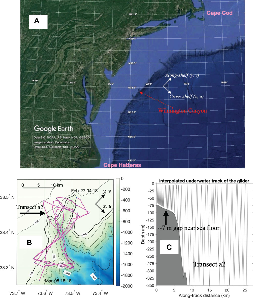
Figure 1 (A) Location of Wilmington Canyon in the Mid-Atlantic Bight. (B) Wilmington Canyon bathymetry with glider survey track (magenta line) during 02/27-03/08/2016. (C) Underwater track taken by the glider at transect a2. The glider used in this study has a maximum diving depth of 350 m. At locations shallower than 350 m, the glider’s altimeter sensor was used during diving to prevent the glider from hitting the seafloor. Thus, the water column within 7 m above the sea floor was generally not sampled.
Wilmington Canyon is the second largest shelf-break submarine canyon (after Hudson Canyon) in the southern MAB. The canyon has an approximately 55° axial bend (Figure 1B): the lower section from the canyon mouth to the bend orients towards the northwest and lays nearly perpendicular to the shelf break (~72°); the upper section from the bend to the canyon head veers to the northeast and lays nearly parallel to the shelf break (~17°). The canyon head intersects the continental shelf at around the 90 m isobath, and the canyon mouth intersects the shelf break at a depth of 150 m. On either side of the canyon axis, the canyon intersects with the continental shelf at the canyon rim. The canyon is approximately 20 km long from the canyon mouth to the canyon head, 10 km wide at the canyon mouth, and has a rim depth of 125 m at the head of the canyon. The depth change along the canyon thalweg from the canyon head to the canyon mouth is approximately 1000 m (www.geomapapp.org; Ryan et al., 2009). The roughly southeast-northwest lower canyon allows an along-shelf flow to interact with canyon topography in a way similar to those previously simulated by idealized numerical models (e.g., Klinck, 1996; Howatt and Allen, 2013). The roughly southwest-northeast alignment of the upper canyon means that canyon flows are channeled in the along-shelf direction. Thus, for Wilmington Canyon, a northeastward (southwestward) incoming along-shelf flow is not only upwelling-favorable (downwelling-favorable) in a classical sense due to the orientation of the lower canyon, but also can flow directly up-canyon (down-canyon) in the upper canyon.
In this study, an underwater glider was deployed in Wilmington Canyon during February 27 - March 8, 2016. During this time period, the MAB experienced nine days of upwelling-favorable winds followed by four days of downwelling-favorable winds. The glider fortuitously obtained hydrographic evidence of consecutive canyon upwelling and downwelling in Wilmington Canyon. To place the glider observations in a greater spatial and temporal context, we utilized a numerical model with realistic forcing and bathymetry. The model allowed us to investigate the cycle of upwelling and downwelling events and compare it with the glider observations. The rest of the paper is organized as follows. Section 2 includes a presentation of the glider survey design and glider configuration, as well as an outline of the numerical modeling system and model setup. In section 3, evidence of the consecutive occurrences of sub-tidal upwelling and downwelling is presented based on the glider observations (sections 3.1.1, 3.1.2.) and numerical simulation (sections 3.1.2, 3.1.3). Then, the development and receding of a canyon-upwelled dense water overflow is described based on model results (sections 3.2., 3.3). The results are discussed in section 4, and key findings are summarized in section 5.
2 Methods
2.1 Glider Survey Design and Glider Configuration
A 350 m Slocum G2 glider “Amelia” was used to survey Wilmington Canyon during February 27 - March 8, 2016 (Figure 1). The glider repeated the “figure 8” shaped survey pattern 3 times (Figure 1B): a transect across the upper canyon, a transect across the lower canyon, a transect parallel to the shelf break, then a transect along the lower canyon. The glider was equipped with the Sea-Bird Scientific’s pumped glider conductivity temperature and depth (CTD) sensor. The CTD sensor was factory calibrated in June 2015 prior to deployment. After the glider was recovered, full resolution delayed-mode temperature, conductivity, and pressure data were extracted from the CTD sensor and thermal lag correction algorithms were applied following Garau et al. (2011). Absolute Salinity and potential density were calculated using Thermodynamic Equation of Seawater 2010 (TEOS-10) provided by the Gibbs SeaWater (GSW) Oceanographic Toolbox (McDougall and Barker, 2011). The glider was also equipped with the following sensors: Sea-Bird Scientific’s EcoPUCK triplet fluorometer with chlorophyll-a, colored dissolved organic matter (CDOM), optical backscatter (700 nm) sensors, and an Aanderaa Optode for measuring dissolved oxygen. In this study, we used the temperature, salinity, and density data at the three repeated transects across the lower canyon, as well as those at the three repeated transects along the lower canyon.
An underwater glider dives and climbs in the water column by changing buoyancy while being propelled forward by the normal force acting on its wings (Webb et al., 2001). Typically, a Slocum glider dives and climbs at ~26° angle from the horizontal plane, at nominal vertical speeds of 0.15 ± 0.04 m/s, and horizontal speeds of 0.25 ± 0.06 m/s through the water. During a 350m deep “yo” consisting of one dive and one climb, which takes approximately 80 minutes, a glider moves laterally by ~1.4 km (assuming no currents) while making ~2400 measurements at a sampling rate of 0.5 Hz. At locations with bathymetry shallower than 350 m, the glider’s downward facing altimeter sensor was used during the downcast to prevent the glider from hitting the seafloor. The glider would inflect from dive to climb at about 7 m above the sea floor. Thus, the water column within 7 m above the bottom was generally not sampled (Figure 1C).
2.2 Numerical Modeling Using the SCHISM Model
To place the observations in larger spatial and temporal contexts, we conducted numerical modeling experiments using the Semi-implicit Cross-scale Hydroscience Integrated System Model (SCHISM, Zhang et al., 2016). SCHISM has been used in multiple studies of the coastal ocean of the U.S. east coast (e.g., Ye et al., 2019; Liu et al., 2020), as well as in a study of the submarine canyons in the Black Sea (Brovchenko and Maderich, 2011). SCHISM is based on unstructured horizontal grids and flexible vertical grids, thus it can represent the complex 3D topography while avoiding artifacts like “staircase-like” bathymetry (Zhang et al., 2016). The pressure gradient force error (Haney, 1991) is effectively reduced using the localized and hybridized vertical grid that lowers the coordinate slopes (Zhang et al., 2016). Other major characteristics of SCHISM include a hybrid finite element/volume formulation, semi-implicit time-stepping, implicit vertical advection scheme for transport (TVD2; Ye et al., 2019), 3rd order Weighted Essentially Non-Oscillatory (WENO) transport in the horizontal dimension (Ye et al., 2019), an efficient and accurate Eulerian-Lagrangian algorithm for momentum advection, horizontal viscosity scheme (including bi-harmonic viscosity) to effectively remove inertial spurious modes without introducing excessive dissipation, etc. For detailed information about SCHISM, please refer to http://schism.wiki. The model implementation was designed to represent the hydrodynamical processes inside Wilmington Canyon, as well as the adjacent outer shelf, shelf-break, and continental slope regions. To achieve this, the model’s domain size, bathymetry, horizontal resolutions, vertical layer configuration, boundary conditions, forcing conditions, simulation time, spin-up time, and time step were all considered.
The model domain covered the US east coast from Georgia to Massachusetts (Figure 2A) and used the GMRT (Ryan et al., 2009) v3.7 bathymetry data (which has 133 m gridded resolution) that has not been smoothed. Overall, the model grid included over 240,000 nodes and 480,000 triangular elements. The model’s horizontal resolution was relatively uniform and high along the shelf-break in the southern and central MAB (Figure 2A). Along the shelf-break isobath (150 m) from ~50 km south of Norfolk Canyon to ~50 km north of Wilmington Canyon, the resolution was ~400 m (Figures 2A, B); in and around Hudson Canyon the resolution was ~1 km; in general, the resolution was 2-3 km at the coast (except in coastal estuaries such as the Chesapeake Bay where the resolution was increased) and 3-8 km at the open ocean boundary. In the vertical direction, depending on water depth, the model has up to 55 levels in the hybrid sigma-z (SZ) vertical grid with enhanced vertical resolutions at the surface and bottom (Figures 2C, D). The bottom layer thickness was generally 0.1-5 m over the continental shelf, shelf-break, slope, and canyons. The high horizontal resolution was designed to capture physical processes within and around the canyons. The intensified vertical resolution near the bottom was designed to capture topographical processes.
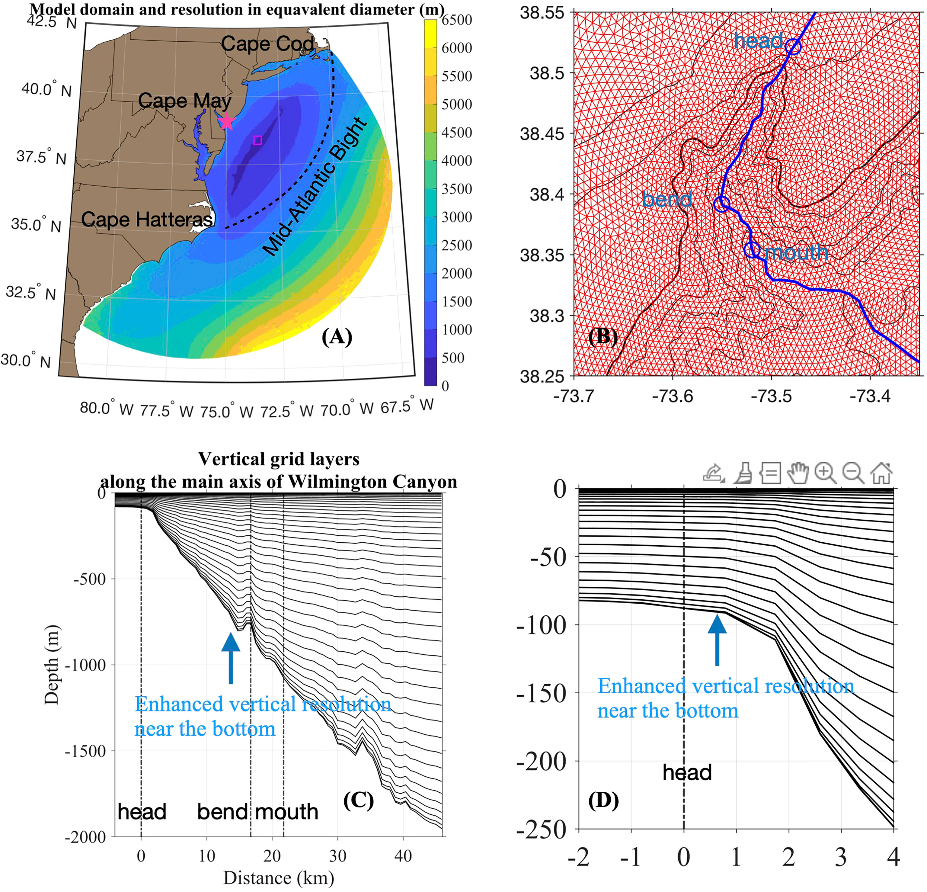
Figure 2 (A) SCHISM model domain and horizontal resolution in equivalent diameter. The model uses >24,000 horizontal nodes, >48,000 unstructured triangular grids, with 350-1000 m resolution over the submarine canyons and adjacent shelf and slope. Location of Wilmington Canyon is indicated by the magenta box. (B) Model mesh over the Wilmington Canyon. Blue line indicates a transect along the canyon’s main axis. Visualization of model vertical layers (C) along the axis of Wilmington Canyon, and (D) zoomed in near the canyon head. There are up to 55 vertical layers depending on water depth. Relatively high vertical resolution is set up for near the surface and bottom. The thickness of the bottom model layer is generally 0.1-5 m over the shelf, shelf-break, and canyon.
Our numerical simulation was subjected to relatively realistic atmospheric and oceanic conditions. It was initialized with conditions of temperature, salinity, and sub-tidal horizontal velocities from a data-assimilative global ocean model - the HYbrid Coordinate Ocean Model (HYCOM), Global Ocean Forecasting System (GOFS) 3.1. This HYCOM model had a 1/12-degree resolution which does not resolve the bathymetry of submarine canyons. At the open ocean boundary of our SCHISM model, a 1.5 degree nudging zone was set, and boundary conditions were forced by the temperature, salinity, and de-tided horizontal velocities from HYCOM, as well as by the tidal elevations and tidal currents from the FES2014 tides database (standard case with Tide). For atmospheric forcing, our implementation included winds, heat fluxes, precipitation, and evaporation from the North American Regional Reanalysis model (NARR, 32 km resolution). Finally, our model took inputs of daily freshwater discharge based on U.S. Geographical Survey (USGS) gauge data for the four major estuaries in the MAB, i.e., Chesapeake Bay, Delaware Bay, Hudson River, and Connecticut River. Altogether, these relatively realistic (as opposed to idealized) atmospheric and oceanic conditions allow us to simulate the hydrodynamics inside Wilmington Canyon and on the adjacent shelf during the study period. In addition, we performed a simulation that excluded tidal forcing at the open boundary (No-Tide case) to investigate how the sub-tidal wind-forced phenomena and tide-forced phenomena are superimposed, and whether the phenomena can be separated in time.
The SCHISM model simulations started on January 1 and ended on March 31, 2016. The spin up period was five days. Results representing February 24 - March 8, 2016, were used in this study. The model used a non-split time step of dt = 120 s. Each model day simulation took about 25 minutes using 300 cores (1324 Xeon “Broadwell” cores) on a High-Performance Computing system (the Bora cluster on SciClone at William & Mary). The model outputs were saved every 2 hours or 12 times daily. Altogether, the above configurations allowed us to investigate the hydrodynamics inside Wilmington Canyon and over the region surrounding the canyon.
3 Results
Observed evidence for a cycle of upwelling and downwelling events is presented in section 3.1, including hydrographic transects within Wilmington Canyon from the glider survey, and the records of winds and water level at a coastal observation station. In section 3.2, we validate the SCHISM implementation by comparing the modeled hydrodynamics to observations. Then in section 3.3, the modeled results from within Wilmington Canyon are provided to examine how the hydrodynamics at the canyon responded to forcing conditions through different phases of the upwelling and downwelling cycle, and to visualize the upwelling and downwelling flows inside Wilmington Canyon. Lastly in section 3.4, the model results for a canyon-upwelled dens water overflow on the shelf, which was generated from the main head of Wilmington Canyon, are presented.
3.1 A Cycle of Upwelling and Downwelling in Wilmington Canyon Shown by Observations
We inferred that a cycle of canyon upwelling and downwelling occurred in Wilmington Canyon during February 27-March 8, 2016, based on repeated glider hydrographical transects. This inference was supported by the records of winds and water level at the NOAA station 8536110 at Cape May, NJ (~100 km shoreward of Wilmington Canyon).
3.1.1 In Situ Evidence From the Glider Survey
Three distinctive water masses comprising the upper 350 m of the water column in and around Wilmington Canyon were observed during the glider survey. To illustrate this, the temperature and salinity data, and associated T/S diagrams at a glider transect along the lower canyon are shown in Figure 3. From surface to bottom, we identified the low-temperature (~ 10 °C) and low-salinity (<34.5) winter shelf water (WSW), the high-temperature (~14 °C) and high-salinity (≥ 35.5) upper slope water (USW), and the low-temperature (~9°C) and high-salinity (~35.3) intermediate slope water (ISW).
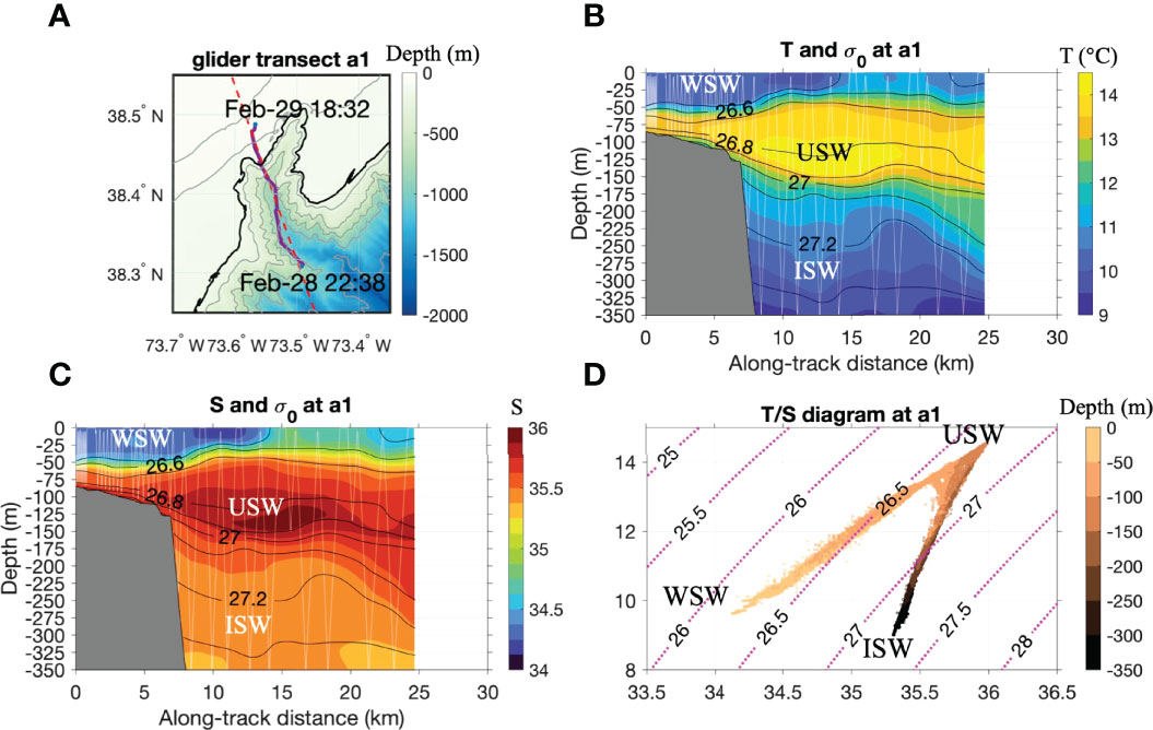
Figure 3 Water masses in the upper 350 m in Wilmington Canyon shown by data at glider transect a1. (A) Purple line indicates glider transect a1. Red dashed line indicates where SCHISM model output was extracted in Figure 6. (B, C) Spatially interpolated fields of temperature and salinity, contours are isopycnals. (D) T/S diagram based on glider data. Three distinctive water masses comprised the upper 350 m of the water column in and around Wilmington Canyon during the glider survey. From surface downward, there were the low-temperature (~ 10°C) and low-salinity (<34.5) winter shelf water (WSW), the high-temperature (~14°C) and high-salinity (≥ 35.5) upper slope water (USW), and the low-temperature (~9°C) and high-salinity (~35.3) intermediate slope water (ISW). Each water mass is shown as an end member in the T/S diagram.
By inspecting the spatial distribution of the three water masses at each glider transect and comparing the changes in water column structure between repeated transects (Figure 4), we could identify that a canyon upwelling event was immediately followed by a downwelling event. It is worth mentioning that a glider transect in this survey typically took 20-30 hours to complete, and the isopycnals below 150 m depth (e.g. σ0 = 27.2 kg m-3) within each glider transect showed semi-diurnal tidal time scale oscillations. Above 150 m, the water column in the canyon is more strongly influenced by surface and frontal processes and the tidally driven semi-diurnal variability is less obvious. While we cannot completely separate spatial variability from temporal variability in the glider observations, in section 3.3, we will use the SCHISM output at a fixed location to show the phases of the upwelling and downwelling events, and the daily mean (tidally averaged) spatial distributions of temperature and velocities across the entire canyon. Regardless of the phases of the tide, comparisons between repeated glider transects show that both the upwelling and downwelling events lasted for several days.
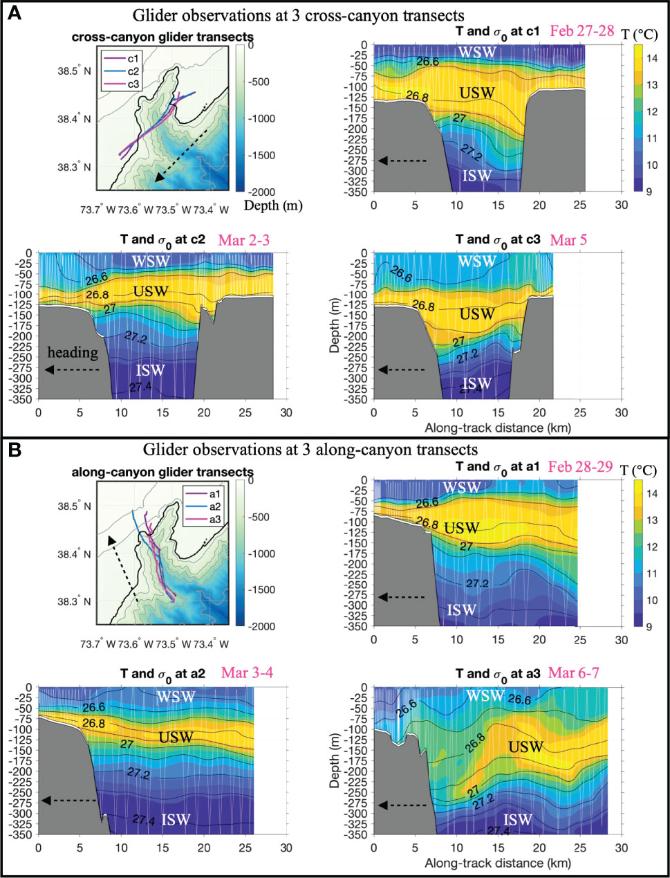
Figure 4 Interpolated temperature (color) and density (contours) fields at (A) three repeated cross-canyon transects and (B) three repeated along-canyon transects from the glider survey. Typically in this mission, a glider transect took 20 to 30 hours to complete. Thin white lines in the temperature transects indicate glider tracks. Dashed black arrows indicate the glider’s heading. The cross-canyon transects c1, c2 and c3 were conducted February 27-28, March 2-3, and March 5, 2016, respectively. The along-canyon transects In a1, a2 and a3 were conducted on February 28-29, March 3-4, and March 6-7 respectively.
Temporal changes between the three cross-canyon transects across the lower canyon (Figure 4A) showed a sequence of water upwelling and downwelling. The transects c1, c2 and c3 were conducted February 27-28, March 2-3, and March 5, 2016, respectively. From transect c1 to transect c2, which were separated by about three days, the ISW layer rose by 50-70 m, consistent with upwelling. From transect c2 to transect c3, which were separated by about two days, the ISW layer fell by 50-70 m, consistent with downwelling.
Next, spatial and temporal varying water column structure at the three glider transects along the lower canyon (Figure 4B) also revealed the same sequence of upwelling and downwelling. The examination here focused on the water column below 100 m depth, especially on the σ0 = 26.8-27.2 kg m-3 isopycnals in the lower portion of USW and upper portion of ISW. In transects a1 (February 28-29) and a2 (March 3-4), the isopycnals tilted upward from the canyon mouth toward the shelf by about 80 m, indicative of upwelling. In transect a3 (March 6-7), the water layers tilted downward from the canyon mouth towards the shelf by about 80 m, indicative of downwelling.
3.1.2 Supporting Evidence From Records of Winds and Water Level at Cape May, NJ
Wind and water level data from the NOAA station 8536110 at Cape May, NJ (~100 km shoreward of Wilmington Canyon) were examined to characterize forcing conditions over the MAB coastal ocean (Figure 5). For most of the time during February 25 - March 3, winds were northwesterly or southwesterly (Figure 5A), i.e. upwelling-favorable. Corresponding to the upwelling winds, the measured water level was lower than predicted astronomical tide (Figure 5B), indicating a sea level set-down at the coast. Then during March 4-7, winds were northeasterly or northerly (Figure 5A), i.e. downwelling-favorable. Corresponding to the downwelling-favorable winds, measured water level was higher than predicted astronomical tide (Figure 5B), indicating a sea level set-up at the coast. The above temporal changes of wind directions and sea level suggest that forcing conditions over the MAB coastal ocean were upwelling-favorable when upwelling was observed in Wilmington Canyon by the glider, and forcing conditions changed to be downwelling-favorable when downwelling was observed in Wilmington Canyon. In section 3.3.1, we will use results from SCHISM to examine how the hydrodynamics at Wilmington Canyon responded to forcing conditions through different phases of the upwelling and downwelling events.
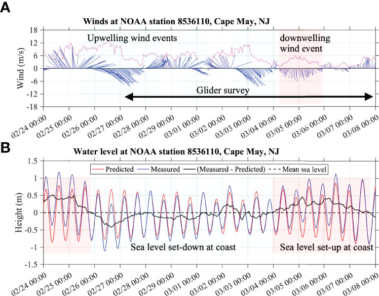
Figure 5 (A) Wind and (B) water level data from the NOAA station 8536110 at Cape May, NJ (~100 km shoreward of Wilmington Canyon). For most of the time during February 25 - March 3, winds were northwesterly or southwesterly (A), i.e. upwelling-favorable. Corresponding to the upwelling winds, the measured water level was lower than predicted, indicating a sea level set-down at the coast. Then during March 4-7, winds were northeasterly or northerly, i.e., downwelling-favorable. Corresponding to the downwelling-favorable winds, measured water level was higher than predicted, indicating a sea level set-up at the coast.
3.2 Model-Data Comparison
To validate the model, we first compared the modeled results from SCHISM with glider observations in terms of the T/S identities and spatial distribution of water masses within the canyon (Figure 6A). As an example, the modeled temperature and salinity data were extracted along the lower canyon to compare with observations. The model outputs were extracted at a straight transect which is roughly overlapping with but slightly longer than the glider transect, and at the halftime point between the beginning and end of the glider transect (Figure 3A). Compared to observations, the model underestimated the temperature and salinity of USW by about 0.8 °C and 0.4 respectively, and of ISW by about 1°C and 0.1 respectively (Figure 6A). Nonetheless, the model produced the same three distinctive water masses as observations. More importantly, the modeled spatial distribution pattern of the water masses, i.e. the water column structure, was consistent with that of observed: the WSW layer occupied the upper ~50 m of the water column over the outer shelf, and this layer became thinner, warmer, and saltier in farther offshore locations over the canyon; the ISW resided below 200 m within the canyon, but tilted upward from the canyon mouth towards the shelf; the USW was wedged between the WSW and ISW, and was thicker within the canyon, thinner over the shelf. Thus, the modeled results showed the same three water masses as observed, and the modeled spatial distribution of water masses was qualitatively similar to observed.
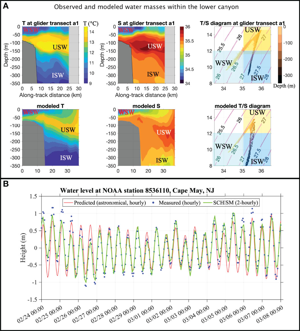
Figure 6 (A) Comparison of the modeled results from SCHISM with glider observations in terms of the T/S identities and spatial distribution of water masses within the canyon. The locations of the glider transect and model transect are shown in Figure 3A. The glider transect was conducted from 22:38 Feb 28 - 18:32 Feb29 (GMT). The modeled results were averaged over 22:00 Feb 28 - 18:00 Feb 29. Bathymetry in glider transects was based on glider altimetry data. Bathymetry in modeled transects was based on GMRT data. (B) Comparison of the modeled water level by SCHISM with the predicted (based on astronomical tides) and measured water level at the NOAA station 8536110 at Cape May, NJ.
We also compared the modeled water level by SCHISM with the predicted (based on astronomical tides) and measured water level at the NOAA station 8536110 at Cape May, NJ (Figure 6B). The SCHISM model generally reproduced the measured water level in terms of tidal phases, and subtidal deviation from predicted water level. In particular, similar to the observed water level, the SCHISM water level was lower than the predicted water level during the upwelling period (e.g., on February 27), and higher than predicted during the downwelling period (e.g., on March 5). The above comparisons indicate that the modeled sea level response was consistent with observations.
The above validations gave us the confidence to use the SCHISM model to examine how the hydrodynamics at the canyon responded to forcing conditions through different phases of the upwelling and downwelling events, to visualize the upwelling and downwelling flows inside Wilmington Canyon, and to inspect the hydrodynamics on the adjacent shelf during the cycle of upwelling and downwelling event.
3.3 Modeled Upwelling and Downwelling Events Inside Wilmington Canyon
3.3.1 Temporal Evolution of the Upwelling and Downwelling Events
Time series of forcing conditions and flow responses at the canyon head (Figure 7) suggest that the canyon upwelling event lasted for 8.5 days from February 25 to March 4, 2016, persisted through multiple tidal cycles, and consisted of a 2-day ramp-up phase, a 5-day quasi-steady phase, and a 1.5-day relaxation phase when wind speeds were reduced. The ensuing downwelling event lasted for 3.5 days from March 4-7, and consisted of 1.5 days of ramp-up, followed by 2 days of relaxation when both winds and currents relaxed back toward zero.
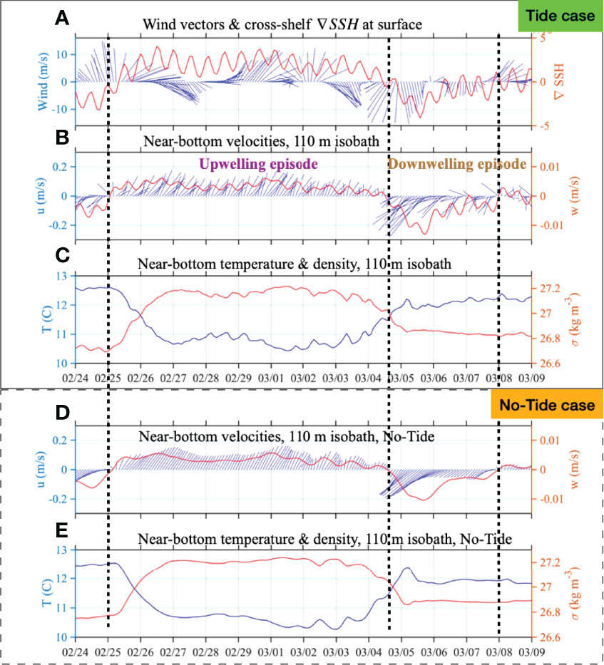
Figure 7 Time series of forcing conditions and flow responses at the canyon head. The point from where the model outputs are extracted is located at about 10 m above bottom at 110 m isobath near the canyon head: (A) wind vectors and cross-shelf SSH gradient (positive is seaward), (B) near bottom velocities (full forcing with tides), (C) near bottom temperature and density, (D) near bottom velocities (no tides), and (E) near bottom temperature and density (no tides). The canyon upwelling event lasted for 8.5 days from February 25 to March 4, 2016, persisted through multiple tidal cycles, and consisted of a 2-day ramp-up phase, a 5-day quasi steady phase, and a 1.5-day relaxation phase. The ensuing downwelling event lasted for 3.5 days from March 4-7, and consisted of 1.5 days of ramp-up, and 2 days of relaxation.
In the ramp-up phase of upwelling on February 25-26, winds turned from southerly to southwesterly and northwesterly with speeds of 10-15 m/s; during the same period the cross-shelf SSH gradient quickly increased (positive gradient is seaward, which corresponds to sea level set-down at the coast) from 0 to 3 ± 1.5 × 10⁻⁶ (Figure 7A). In response to the changing conditions of wind and SSH gradient, the near-bottom currents at the canyon head (extracted at 10 m above sea floor at the 110 m isobath), which were southwestward before, now turned to be northeastward (i.e. up-canyon), with speed accelerated to about 0.2 m/s (Figure 7B). The vertical flow velocity, w, turned from negative to positive (i.e. upward) at 4 ± 1 mm/s. In the same two days of upwelling ramp-up, water temperature decreased from 12.5 to 10.7 °C, and the water density anomaly increased from 26.7 to 27.2 kg m-3 (Figure 7C). In the following 5-day quasi-steady phase of upwelling, from February 27 to March 2, despite tidal oscillations, westerly winds sustained the positive cross-shelf SSH gradient (Figure 7A). During this phase, near-bottom currents at the canyon head continuously flowed up-canyon at 0.15-0.2 m/s, the vertical velocity remained upward at 3-5 mm/s (Figure 7B), water temperature and density anomalies remained steady at 10.5-11 °C, and 27.1-27.2 kg m-3, respectively (Figure 7C).
Then during the relaxation phase of upwelling on March 3 and first half of March 4, northwesterly winds gave way to northeasterly winds, cross-shelf SSH gradient decreased to about 0 (Figure 7A), near-bottom flow and its vertical velocity both decreased to about 0 as well (Figure 7B), water temperature increased to 11.5 °C, and density anomaly decreased to 27.0 kg m-3 (Figure 7C). In the transition phase between the upwelling event and downwelling event around 00:00 on March 4, the directions of winds and SSH gradient changed from being upwelling- to downwelling-favorable. Throughout March 4, northeasterly and northerly wind speeds continued to increase, and reached 10-16 m/s (Figure 7A) before decreasing on March 5 (Figure 7A).
In the second half of March 4 and first 18 hours of March 5, cross-shelf SSH gradient became increasingly negative from 0 to -4 × 10⁻⁶ (Figure 7A). At the same time, near the bottom at the canyon head (10 m above sea floor at the 110 m isobath), down-canyon currents increased from 0 to 0.35 m/s, vertical velocity accelerated from 0 to -13 mm/s (Figure 7B), temperature increased to about 12 °C, and the density anomaly decreased to 26.8 kg m-3 (Figure 7C). From the end of March 5 to March 7, as wind speed gradually decreased, the cross-shelf SSH gradient and current velocities all gradually decreased, though the temperature and density anomalies roughly stayed constant.
3.3.2 Effect of Tides on Canyon Upwelling and Downwelling
The ocean’s response to subtidal and tidal forces is a superimposition of various processes operating on different time scales. Due to the speed of glider’s motion, their observations tend to convolve mesoscale spatial variability with temporal variability driven by tides. However, we can easily separate subtidal events and tidal variabilities in numerical models. Time series at the canyon head from the Tide and No-Tide simulations showed the same sub-tidal upwelling and downwelling events in response to changes in winds and cross-shelf SSH gradients. Tidal oscillations were superimposed on the sub-tidal events in the Tide case (Figures 7B, C) and were absent in the No-Tide case (Figures 7D, E).
In the Tide case, time series of near-bottom velocities, temperature, and density all displayed the sub-tidal events of upwelling and downwelling as well as tidal oscillations (Figures 7B, C). The sub-tidal upwelling event (February 25 - March 4) corresponded to 8.5 days of upwelling-favorable southwesterly and northwesterly winds and persistently positive cross-shelf SSH gradients (Figure 7A). The sub-tidal downwelling event (March 4-7) corresponded to 3.5 days of downwelling-favorable northerly and northeasterly winds and persistently negative cross-shelf SSH gradients. Tidal oscillations were mainly semi-diurnal, and superimposed on the sub-tidal signals (Figures 7A–C).
In the No-Tide case, where tidal forcing was turned off, the sub-tidal events of canyon upwelling and downwelling, demonstrated by the time series of velocities, temperature, and density, still occurred in the same periods and at nearly the same magnitudes (Figures 7D, E).
These results suggest that observed and modeled canyon upwelling and downwelling events were sub-tidal processes driven by winds and pressure gradients (associated with SSH gradients), and they would occur with or without tidal forcing.
3.3.3 Spatial Views of Upwelling and Downwelling Flows
The strongest flows during both upwelling and downwelling were located at the canyon head. During the upwelling event, upwelling flow delivered ISW and USW from 215-100 m depths through the canyon head onto the outer shelf; in the ensuing downwelling event, the previously upwelled water flowed down-slope inside the canyon in bottom-intensified currents.
The modeled horizontal velocity hvel and vertical velocity w at the shelf-break depth of z=150 m are shown in Figure 8. On March 1, at the peak of the upwelling period, maximum velocities (up-canyon hvel and upward w) were at the canyon head (Figures 8A, C). On March 5, at the peak of the downwelling period, the maximum velocities (down-canyon hvel and downward w) spread near the canyon head and along the northeast flank of the upper canyon (Figures 8B, D). Comparing the two scenarios (March 1 vs. March 5), downwelling had maximum hvel >0.3 m/s and maximum w >15 mm/s, both about twice those calculated during upwelling.
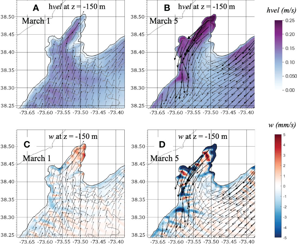
Figure 8 Modeled fields of (A, B) horizontal velocity hvel and (C, D) vertical velocity w at the shelf-break depth of z = -150 m. hvel vectors were interpolated from unstructured model mesh (Figure 2B) to coarser structured grids for visualization. On March 1, at the peak of the upwelling period, maximum velocities (up-canyon hvel and upward w) were at the canyon head (Figures 8A, C). On March 5, at the peak of the downwelling period, the maximum velocities (down-canyon hvel and downward w) spread near the canyon head and along the northeast flank of the upper canyon (Figures 8B, D). Comparing the two scenarios (March 1 vs. March 5), downwelling had maximum hvel >0.3 m/s and maximum w >15 mm/s, both about twice those calculated during upwelling.
Transect views of the along-canyon component of horizontal velocity, vertical velocity, and temperature for the transect along the main axis of Wilmington Canyon are shown in Figure 9. On March 1, in the quasi-steady maximum phase of the upwelling event, the canyon upwelling flow was characterized by up-canyon horizontal velocity (Figure 9A) and upward vertical velocity (Figure 9C). Near the canyon head, the flow’s horizontal velocity reached 0.4-0.5 m/s, and vertical velocity reached about 5 mm/s. This canyon-upwelling flow delivered the lower layers of USW and upper layers of ISW from inside the canyon onto the outer continental shelf (Figure 9E). The deepest source of the upwelled water was from a depth of 215 m near the canyon mouth, which was about 50 m below the canyon rim at the canyon’s mouth. On March 5, in the downwelling maximum phase, there were bottom-intensified currents flowing down-slope inside the canyon near the canyon head with horizontal velocity of 0.3 m/s (Figure 9B) and downward vertical velocity of 15 mm/s (Figure 9D). The previously upwelled dense slope water now fell to 200-350 m depths within the canyon (Figure 9F).
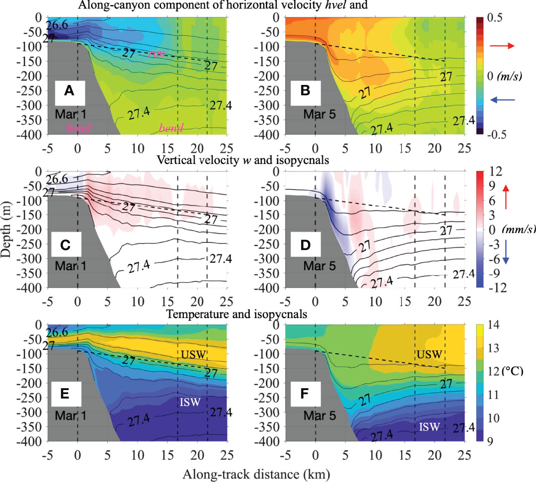
Figure 9 Transect views of daily mean (A, B) along-canyon component of horizontal velocity, (C, D) vertical velocity w, and (E, F) temperature for the transect along the main axis of Wilmington Canyon (location of the transect is shown in Figure 2B). On March 1, during canyon upwelling, flow was characterized by up-canyon horizontal velocity and upward vertical velocity. The lower layers of USW and upper layers of ISW from inside the canyon upwelled onto the outer continental shelf. The deepest source of the upwelled water was from about 215 m depth near the canyon mouth, which was about 50 m below the canyon rim at the canyon’s mouth. On March 5, during canyon downwelling, there were bottom-intensified currents flowing down-slope inside the canyon near the canyon head with horizontal velocity of 0.3 m/s and downward vertical velocity of 15 mm/s. The previously upwelled dense slope now fell to 200-350 m depths within the canyon.
3.4 A Canyon-Upwelled Dense Water Overflow Revealed by the Model
The model simulation allowed us to study the fate, dynamics, and impact of the canyon-upwelled slope water on the shelf. As a result of upwelling at Wilmington Canyon, a dense water overflow made of relatively cold and dense ISW was found at the upper canyon and the bottom of the outer shelf northeast of the canyon. During the upwelling event, the overflow water was advected northeastward with shelf currents and grew wider in the cross-shelf direction. In the ensuing downwelling event, shelf currents changed to be southwestward, and the dense overflow water receded back into the canyon.
3.4.1 Development and Recession of the Canyon-Upwelled Dense Water
The development of a canyon-upwelled dense overflow water containing ISW is shown by the temperature and horizontal velocity vectors calculated for the model layer right above the sea floor (Figure 10A). Before the upwelling event on February 24, the bottom of the shelf was still occupied by USW (T>12°C). By day 2 of upwelling, on February 26, the canyon-upwelled ISW (T<12°C) was seen at the bottom of the shelf just north of the canyon head. This dense water was sustained on the shelf for the following six days of the upwelling event, during which time it flowed northeastward in the along-shelf direction and spread in the cross-shelf direction. As the dense water overflow developed, the bottom temperature on the downstream shelf between the 75-100 m isobaths cooled from 12-13 °C on February 24 to 10-11 °C on March 1. At the peak of upwelling on March 1, the cold overflow covered > 90% of the outer shelf between 75-150 m isobaths. The only shelf area that remained to be occupied by warmer USW (T>12°C) was located at the corner northeast of the canyon mouth.
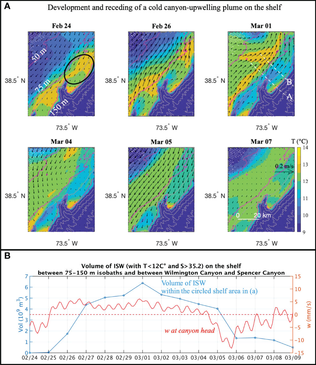
Figure 10 (A) Daily mean temperature and horizontal velocity vectors calculated for the model layer right above the sea floor. A canyon-upwelled dense water overflow consisting of cold ISW developed on the shelf northeast of Wilmington Canyon during the upwelling phase, and the dense water receded from the shelf during the downwelling phase. (B) Daily mean volume of ISW (blue line) calculated within the circled shelf area northeast of Wilmington Canyon (between 75-m and 150-m isobaths). Red line is the 2-hourly vertical velocity at the canyon head.
The upwelling transported a substantial volume of ISW on to the shelf (Figure 10B). Within the area of outer shelf between 75-150 m isobaths and between Wilmington Canyon and Spencer Canyon, the volume of canyon-upwelled ISW with T<12 °C and S>35.2 increased from zero on February 24-25 to 4.5 × 10⁹m3 on February 27, reached >6 × 10⁹m3 on March 1, and the volume of ISW on the shelf remained above 4.5 × 10⁹m3 until the end of the upwelling period on March 4.
In the downwelling event (March 4-7) that directly followed the upwelling event (February 25 - March 4), the canyon-upwelled ISW receded from the shelf. During this period, the directions of winds and SSH gradients (Figure 7A) reversed to be downwelling-favorable, and the shelf currents flowed southwestward (Mar 5, Figure 10). Consequently, ISW was no longer being transported from within Wilmington Canyon onto the shelf, and the remaining ISW on the shelf was advected southwestward back towards the canyon. The dense ISW on the shelf decreased in terms of horizontal extent (Figure 10A) and total volume (Figure 10B).
3.4.2 Impact of Canyon-Upwelling Dense Water on Shelf Circulation
The canyon-upwelled dense water overflow induced an interesting velocity structure during the upwelling event. This is illustrated by the daily mean velocity distributions from March 1 (Figure 11). In terms of along-shelf velocity (Figures 11C, D), there was a northeastward-flowing frontal jet with speed > 0.5 m/s at the shoreward density front associated with the dense overflow (above 75 m isobath). Near the canyon head, the core of this frontal jet was about 7 km wide in the cross-shelf direction and was about 30 m thick within the water column at 10-40 m above bottom (Figure 11C). Farther downstream (to the northeast), at 15 km away from the canyon, the core of the jet was approximately 10 km wide, and 10-15 m thick (Figure 11D). There was also secondary cross-shelf circulation that allowed the overflow water to expand both shoreward and seaward during the upwelling period. Near the canyon head, the daily mean cross-shelf circulation on March 1 was characterized by up to 0.1 m/s shoreward velocity on the shoreward and lower half of the overflow, and up to 0.05 m/s seaward velocity on the seaward and upper half of the overflow water (Figure 11E). Farther downstream, the cross-shelf circulation was characterized by <0.05 m/s shoreward velocity on the lower half of the overflow, and up to 0.2 m/s seaward velocity on the upper half of the overflow and in the water column above (Figure 11F). Both the along-shelf frontal jet and secondary cross-shelf circulation are indicative of density-driven dynamics by the canyon-upwelled overflow.
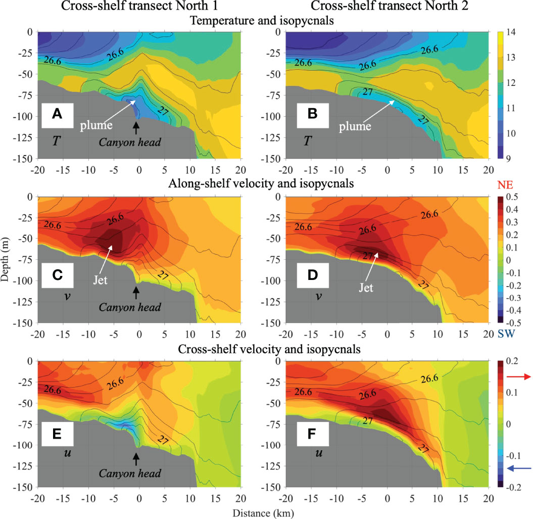
Figure 11 Cross-shelf transect views of daily mean (A, B) temperature, (C, D) along-shelf velocity, and (E, F) cross-shelf velocity on March 1 during the upwelling event, contours are isopycnals. The locations of transects A and B are shown in Figure 10 (Mar 1). The positive direction of along-shelf velocity is pointing northeastward, of cross-shelf velocity is pointing seaward. The cold and dense canyon-upwelled dense water overflow was seen at the canyon head. A subsurface along-shelf frontal jet was located at the shoreward flank of the canyon-upwelled overflow water. The frontal jet flowed towards northeast. At transect A, the dense water also expanded both shoreward and seaward in the cross-shelf direction.
3.4.3 Dynamics Associated With the Dense Overflow Frontal Jet
To investigate the dynamical drivers of the frontal jet associated with the dense overflow, we focus on a cross-shelf transect just northeast of the canyon head labelled as “Northern-1”. During upwelling on February 29, the Northern-1 cross-shelf transect’s isopycnals domed at the head of the canyon due to upwelling of dense overflow water onto the shelf (Figure 12). Such a density distribution caused a shoreward baroclinic horizontal pressure gradient force (HPGF) to develop on the shoreward side of the canyon head, and seaward baroclinic HPGF to develop on the seward side of the canyon head (Figure 12B). Within the overflow water, the baroclinic HPGF was dominant and unbalanced in the cross-shelf direction, likely due to the ageostrophic advection up the canyon (Figure 12F), thus the overflow water spread seaward and shoreward from the canyon head by the cross-shelf baroclinic HPGF (Figure 12F).
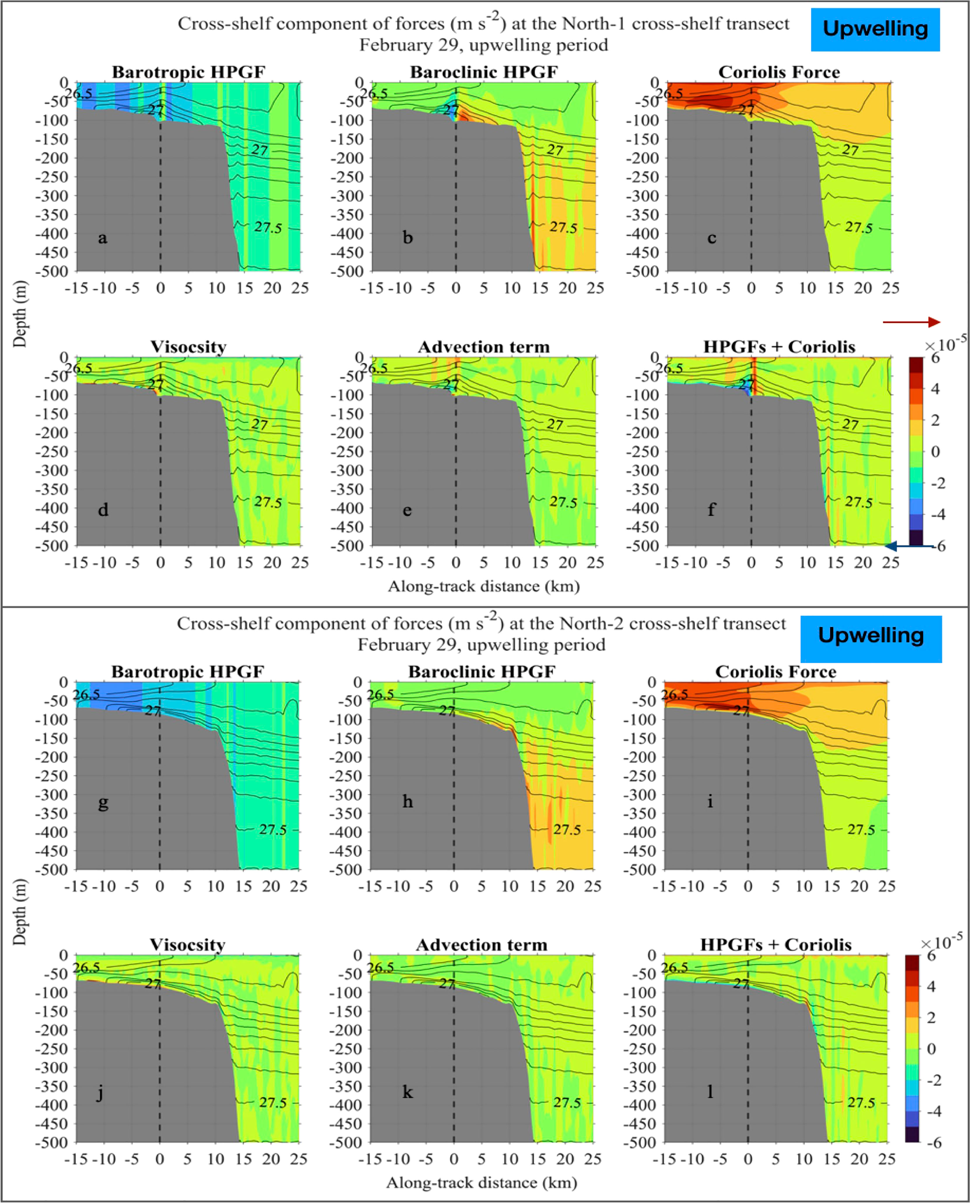
Figure 12 Cross-shelf momentum balance for February 29, 2016 at the North-1 transect just northeast of the head of the canyon (A–F) and the North-2 transect 20 km northeast of the North-1 transect (G–L). (A, G) Barotropic horizontal pressure gradient force. (B, H) Baroclinic horizontal pressure gradient force. (C, I) Coriolis Force. (D, J) Viscosity. (E, K) Advection. (F, L) HPGF + Coriolis.
Meanwhile, on the shoreward side of the canyon head both the baroclinic and barotropic HPGFs were in same direction toward the shore during upwelling; and on the seaward side of the canyon head, they opposed each other. Thus, the total HPGF was greater in magnitude on the shoreward side of the canyon head than the seaward side. Geostrophic balance required a greater Coriolis force on the shoreward side of the canyon head (Figure 12C). This implies that the along-shelf overflow current in the form of a northeastward subsurface baroclinic jet would develop on the shoreward flank of the canyon-upwelled dense water (Figures 11C, D). At the Northern-2 cross-shelf transect farther downstream of the canyon (Figures 12G–L), isopycnals were nearly parallel to the bottom, and the main force terms were in geostrophic balance (Figure 12L). However, the distribution of baroclinic HPGF was still shoreward on the shoreward flank of the dense water, and seaward on the seaward flank of the dense water (Figure 12H). Consequently, the Coriolis force was also greater on the shoreward flank of the dense water here (Figure 12I), thus there was the northeastward subsurface baroclinic jet.
4 Discussion
4.1 Impact of Canyon-Upwelled Dense Water on the Canyon Flow During the Ensuing Downwelling Event
In this study, despite the speeds of shelf currents being about equal during the upwelling and downwelling events (March 1 & 5 in Figure 10), flows within Wilmington Canyon were stronger during the downwelling event than seen in the preceding upwelling event (March 1 & 5 in Figures 8, 9). These results with angled canyon alignment and realistic bathymetry are different idealized modeling studies that showed canyon upwelling would be stronger than canyon downwelling (Klinck, 1996; Spurgin and Allen, 2014; Zhang and Lentz, 2017) under equal-strength background conditions. The parallel alignment of the upper canyon with the shelfbreak means there is a dynamical bias for enhanced gravity assisted down canyon flow. However, the details of such dynamical balances remain a topic of future investigation. In addition, our study of Wilmington Canyon investigated a real-world scenario in which a downwelling event immediately followed an upwelling event. In the upwelling phase, dense slope water was upwelled onto and sustained on the shelf. When the upwelling event ended, and conditions changed to be downwelling-favorable, the previously canyon-upwelled dense water that had been accumulated on the shelf was advected southwestward by the along-shelf shelf currents towards the canyon, which is oriented nearly along-shelf. The canyon-upwelled water then flowed down-slope toward deeper parts of the canyon causing bottom-intensified flow in the upper canyon. This receding of the previous upwelled water enhanced the effect of advection-driven canyon downwelling. As a result, the flow velocities in Wilmington Canyon in the downwelling event were stronger than seen in the preceding upwelling event.
4.2 Canyon Upwelled Dense Overflow Water in the MAB
The canyon-upwelled overflow from Wilmington Canyon resembled those reported in previous studies of canyon upwelling. These previous studies were based on either numerical simulations (e.g. Kämpf, 2009; Kämpf, 2010; Howatt and Allen, 2013; Ramos Musalem, 2020; Saldías and Allen, 2020) or laboratory models (Ramos Musalem, 2020) of idealized straight and smooth canyons that were oriented perpendicular to the shelf-break. In contrast, our study represented Wilmington Canyon and the surrounding area using non-smoothed bathymetry (based on GMRT), and relatively realistic forcing conditions (with inputs of winds, tides, ocean currents, water column structure from data-assimilative models). Despite these differences, our modeling study and previous studies all showed a canyon-upwelled dense water developed on the continental shelf, and a near-bottom frontal jet on the shoreward flank of the upwelled dense water.
A canyon-upwelled dense water overflow consisting of ISW has not been reported in previous observational studies of the MAB. Although intrusions of the warm (>14 °C) USW at the outer shelf is a common feature in the MAB, the presence of colder and denser ISW on the shelf has been rarely observed. This discrepancy between modeling results and existing observations may be attributed to the fact that most hydrographic observations on the shelf avoid the bottom boundary layer (~0-10 m above bottom) and that continuous and high-resolution observations at the canyon heads and right downstream (northeast) of canyons during upwelling events are very rare. As a result, the presence of dense overflow water on the shelf resulting from canyon upwelling events may have consistently escaped previous observational efforts.
In this study, although a hint of ISW was observed on the outer shelf (Figures 3, 4), the glider observations were insufficient to resolve the canyon upwelled overflow shown in the model. An operational reason was that the glider was programmed to avoid hitting the seafloor, therefore the bottom 5-10 m of the water column on the shelf was generally not well sampled. More importantly, the glider survey did not have sufficient spatial coverage on the outer shelf northeast of Wilmington Canyon where the dense water on the shelf would have resided.
In order to capture canyon-upwelled dense water from a shelf-break canyon in the MAB, we have the following recommendation for future observations: (1) high resolution hydrographic observations at the canyon head, especially the near-bottom 20 m northeast of a canyon; (2) conduct the study over a sustained period so that it can capture the episodic event when sub-tidal flows are northeastward over the outer shelf and shelf-break, especially during prolonged (>2 days) and strong (e.g. ≥10 m/s) upwelling-favorable wind events; (3) employ a complimentary set of moored array (profiler moorings capable of profiling from the bottom up to the surface, lined from the canyon head to the downstream shelf) and mobile platforms (gliders, AUVs or shipboard surveys for quick and high-resolution synoptic transects in both the along-overflow and across-overflow directions).
Canyon-upwelled dense overflows are likely important features that have the potential to supply significant quantities of water, salt, and nutrients from continental slope waters to the continental shelf of the MAB. The overflow at Wilmington Canyon characterized in this study had its source water from the ISW, which were located roughly at 150 – 215 m depths. The peak volume of ISW contained in the overflow was estimated to be > 6 × 10⁹m3. Thus, it is reasonable to conclude that submarine canyons may supply a significant quantity of ISW onto the shelf during upwelling events. In addition, ISW is saltier than shelf waters, and has relatively high nutrient concentration (e.g. He et al., 2011), thus upwelled ISW may be a significant source of salt and nutrients from the slope sea to the shelf.
5 Conclusions
We used observations from a glider survey and a numerical model with relatively realistic bathymetry and forcing to analyze a cycle of wind-driven canyon upwelling and downwelling that occurred over Wilmington Canyon in the southern MAB. In this cycle of events, an upwelling event (February 25 - March 3, 2016) was immediately followed by a downwelling (March 4-7, 2016) event. During the upwelling event, winds were upwelling-favorable, sea level increased seaward, shelf currents flowed northeastward, ISW originating from 150-215 m depths within the canyon was channeled onto the shelf, and formed a cold and dense canyon-upwelled overflow on outer continental shelf (75-150 m isobaths) northeast of the canyon. The overflow contained up to 6 × 10⁹m3 of ISW, lowered the bottom temperature of the outer shelf by up to 2°C, and induced a near-bottom frontal jet with speeds over 0.5 m/s. In the ensuing downwelling event, winds were downwelling-favorable, sea level increased landward, shelf-currents were southwestward, and the previously upwelled ISW receded from the shelf to the canyon, causing 0.3 m/s bottom-intensified down-slope currents in the upper canyon near the canyon head. Canyon upwelled dense water overflows have not been reported in previous observational studies of the MAB due to their location specificity and episodic nature. However, they have the potential to supply and entrain significant quantities of water, salt, and nutrients from the slope sea to the continental shelf of the MAB.
Data Availability Statement
The observational data and model outputs used in this study will be made available by the authors, without undue reservation.
Author Contributions
HW conducted glider survey, numerical modeling, data analysis, data visualization, and writing. DG obtained funding, conducted glider survey, participated in data analysis and writing. MF participated in data analysis and writing. CH participated in data analysis and writing. TM participated in data analysis and writing. H-CY participated in numerical modeling and data analysis. YZ participated in numerical modeling, data analysis, and writing. All authors contributed to the article and approved the submitted version.
Funding
We thank the Mid-Atlantic Regional Association Coastal Ocean Observing System (MARACOOS, https://maracoos.org) for funding of this project. We thank the VIMS/SMS Office of Academic Studies for supporting Haixing Wang throughout his Ph.D. study. The work was supported by NOAA grant NA16NOS0120020/5940.
Conflict of Interest
The authors declare that the research was conducted in the absence of any commercial or financial relationships that could be construed as a potential conflict of interest.
Publisher’s Note
All claims expressed in this article are solely those of the authors and do not necessarily represent those of their affiliated organizations, or those of the publisher, the editors and the reviewers. Any product that may be evaluated in this article, or claim that may be made by its manufacturer, is not guaranteed or endorsed by the publisher.
Acknowledgments
We thank captains Sean Fate and PG Ross from the Virginia Institute of Marine Science (VIMS) Eastern Shore Lab, and David Aragon from Rutgers University for their assistance in the glider deployment. We thank William & Mary Research Computing for providing computational resources and technical support (https://www.wm.edu/it/rc). This paper is Contribution No.4102 of the Virginia Institute of Marine Science, William & Mary.
References
Allen S. E., Durrieu de Madron X. (2009). A Review of the Role of Submarine Canyons in Deep-Ocean Exchange With the Shelf. Ocean Sci. 5 (4), 607–620. doi: 10.5194/os-5-607-2009
Allen S. E., Hickey B. M. (2010). Dynamics of Advection-Driven Upwelling Over a Shelf Break Submarine Canyon. J. Geophys. Res. Oceans 115 (C8). doi: 10.1029/2009JC005731
Brovchenko I., Maderich V. (2011). Study of the Role of Underwater Canyons in Sediment Transport From the Black Sea East Coast. Int. J. Comput. Civ. Struct. Eng. 7 (2), 39–46.
Butman B. (1986). North Atlantic Slope and Canyon Study. Volume 2 (Woods Hole, MA (USA: Geological Survey).
Church T. M., Mooers C. N., Voorhis A. D. (1984). Exchange Processes Over a Middle Atlantic Bight Shelfbreak Canyon. Estuar. Coast. Shelf Sci. 19 (4), 393–411. doi: 10.1016/0272-7714(84)90093-3
Connolly T. P., Hickey B. M. (2014). Regional Impact of Submarine Canyons During Seasonal Upwelling. J. Geophys. Res. Oceans 119 (2), 953–975. doi: 10.1002/2013JC009452
Freeland H. J. (1982). A Topographically Controlled Upwelling Center Off Southern Vancouver Island. J. Mar. Res. 40, 1069–1093.
Garau B., Ruiz S., Zhang W. G., Pascual A., Heslop E., Kerfoot J., et al (2011). Thermal Lag Correction on Slocum CTD Glider Data. J. Atmos. Ocean. Technol. 28 (9), 1065–1071. doi: 10.1175/JTECH-D-10-05030.1
Haney R. L. (1991). On The Pressure Gradient Force Over Steep Topography in Sigma Coordinate Ocean Models. J. Phys. Ocean. 21, 610–618.
Harris C. K., Butman B., Traykovski P. (2003). Winter-Time Circulation and Sediment Transport in the Hudson Shelf Valley. Cont. Shelf Res. 23 (8), 801–820. doi: 10.1016/S0278-4343(03)00025-6
He R., Chen K., Fennel K., Gawarkiewicz G. G., McGillicuddy D. J. Jr. (2011). Seasonal and Interannual Variability of Physical and Biological Dynamics at the Shelfbreak Front of the Middle Atlantic Bight: Nutrient Supply Mechanisms. Biogeosciences 8 (10), 2935. doi: 10.5194/bg-8-2935-2011
Hickey B. M. (1997). The Response of a Steep-Sided, Narrow Canyon to Time-Variable Wind Forcing. J. Phys. Oceanogr. 27 (5), 697–726. doi: 10.1175/1520-0485(1997)027<0697:TROASS>2.0.CO;2
Howatt T. M., Allen S. E. (2013). Impact of the Continental Shelf Slope on Upwelling Through Submarine Canyons. J. Geophys. Res. Oceans 118 (10), 5814–5828. doi: 10.1002/jgrc.20401
Hunkins K. (1988). Mean and Tidal Currents in Baltimore Canyon. J. Geophys. Res. Oceans 93 (C6), 6917–6929. doi: 10.1029/JC093iC06p06917
Kämpf J. (2006). Transient Wind Driven Upwelling in A Submarine Canyon: A Process Oriented Modeling Study. J Geophys Res: Oceans 111 (c11).
Kämpf J. (2009). On the Interaction of Time-Variable Flows With a Shelfbreak Canyon. J. Phys. Oceanogr. 39 (1), 248–260. doi: 10.1175/2008JPO3753.1
Kämpf J. (2010). On Preconditioning of Coastal Upwelling in the Eastern Great Australian Bight. J. Geophys. Res. Oceans 115 (C12). doi: 10.1029/2010JC006294
Kämpf J. (2012). Lee Effects of Localized Upwelling in a Shelf-Break Canyon. Cont. Shelf Res. 42, 78–88. doi: 10.1016/j.csr.2012.05.005
Klinck J. M. (1996). Circulation Near Submarine Canyons: A Modeling Study. J. Geophys. Res. Oceans 101 (C1), 1211–1223. doi: 10.1029/95JC02901
Lentz S. J. (2010). The Mean Along-Isobath Heat and Salt Balances Over the Middle Atlantic Bight Continental Shelf. J. Phys. Oceanogr. 40 (5), 934–948. doi: 10.1175/2009JPO4214.1
Lentz S. J., Butman B., Harris C. (2014). The Vertical Structure of the Circulation and Dynamics in Hudson Shelf Valley. J. Geophys. Res. Oceans 119 (6), 3694–3713. doi: 10.1002/2014JC009883
Liu Z., Wang H. V., Zhang Y., Magnusson L., Loftis J. D., Forrest D. (2020). Cross-Scale Modeling of Storm Surge, Tide, and Inundation in Mid-Atlantic Bight and New York City During Hurricane Sandy 2012. Estuar. Coast. Shelf Sci. 233. doi: 10.1016/j.ecss.2019.106544
McDougall T. J., Barker P. M. (2011). Getting Started With TEOS-10 and the Gibbs Seawater (GSW) Oceanographic Toolbox 28.
Ramos Musalem A. K. (2020). Transport Through Submarine Canyons (Doctoral dissertation, University of British Columbia).
Ryan W. B. F., Carbotte S. M., Coplan J. O., O'Hara S., Melkonian A., Arko R., et al (2009). Global Multi-Resolution Topography Synthesis. Geochem. Geophys. Geosyst. 10, Q03014. doi: 10.1029/2008GC002332
Saldías G. S., Allen S. E. (2020). The Influence of a Submarine Canyon on the Circulation and Cross-Shore Exchanges Around an Upwelling Front. J. Phys. Oceanogr. 50 (6), 1677–1698. doi: 10.1175/JPO-D-19-0130.1
She J., Klinck J. M. (2000). Flow Near Submarine Canyons Driven by Constant Winds. J. Geophys. Res. Oceans 105 (C12), 28671–28694. doi: 10.1029/2000JC900126
Spurgin J. M., Allen S. E. (2014). Flow Dynamics Around Downwelling Submarine Canyons. Ocean Sci. 10, 799–819. doi: 10.5194/os-10-799-2014
Webb D. C., Simonetti P. J., Jones C. P. (2001). SLOCUM: An Underwater Glider Propelled by Environmental Energy. IEEE J. Ocean. Eng. 26 (4), 447–452. doi: 10.1109/48.972077
Ye F., Zhang Y., He R., Wang Z., Wang H. V., Du J. (2019). Third-Order WENO Transport Scheme for Simulating the Baroclinic Eddying Ocean on an Unstructured Grid. Ocean Model. 143, 101466. doi: 10.1016/j.ocemod.2019.101466
Zhang W., Lentz S. J. (2017). Wind-Driven Circulation in a Shelf Valley. Part I: Mechanism of the Asymmetrical Response to Along-Shelf Winds in Opposite Directions. J. Phys. Oceanogr. 47 (12), 2927–2947. doi: 10.1175/JPO-D-17-0083.1
Keywords: submarine canyon, shelf-slope exchange, upwelling, downwelling, wind-driven circulation, shelf-break dynamics, Mid-Atlantic Bight, frontal jet
Citation: Wang H, Gong D, Friedrichs MAM, Harris CK, Miles T, Yu H-C and Zhang Y (2022) A Cycle of Wind-Driven Canyon Upwelling and Downwelling at Wilmington Canyon and the Evolution of Canyon-Upwelled Dense Water on the MAB Shelf. Front. Mar. Sci. 9:866075. doi: 10.3389/fmars.2022.866075
Received: 30 January 2022; Accepted: 16 May 2022;
Published: 16 June 2022.
Edited by:
Hiroaki Saito, The University of Tokyo, JapanCopyright © 2022 Wang, Gong, Friedrichs, Harris, Miles, Yu and Zhang. This is an open-access article distributed under the terms of the Creative Commons Attribution License (CC BY). The use, distribution or reproduction in other forums is permitted, provided the original author(s) and the copyright owner(s) are credited and that the original publication in this journal is cited, in accordance with accepted academic practice. No use, distribution or reproduction is permitted which does not comply with these terms.
*Correspondence: Donglai Gong, Z29uZ0B2aW1zLmVkdQ==