Prediction of Pan-Arctic Sea Ice Using Attention-Based LSTM Neural Networks

Within the rapidly changing Arctic region, accurate sea ice forecasts are of crucial importance for navigation activities, such as the planning of shipping routes. Numerical climate models have been widely used to generate Arctic sea ice forecasts at different time scales, but they are highly dependent on the initial conditions and are computationally expensive. Recently, with the increasing availability of geoscience data and the advances in deep learning algorithms, the use of artificial intelligence (AI)-based sea ice prediction methods has gained significant attention. In this study, we propose a supervised deep learning approach, namely attention-based long short-term memory networks (LSTMs), to forecast pan-Arctic sea ice at monthly time scales. Our method makes use of historical sea ice concentration (SIC) observations during 1979–2020, from passive microwave brightness temperatures. Based on the persistence of SIC anomalies, which is known as one of the dominant sources of sea ice predictability, our approach exploits the temporal relationships of sea ice conditions across different time windows of the training period. We demonstrate that the attention-based LSTM is able to learn the variations of the Arctic sea ice and can skillfully forecast pan-Arctic SIC on monthly time scale. By designing the loss function and utilizing the attention mechanism, our approach generally improves the accuracy of sea ice forecasts compared to traditional LSTM networks. Moreover, it outperforms forecasts with the climatology and persistence based empirical models, as well as two dynamical models from the Copernicus Climate Change Service (C3S) datastore. This approach shows great promise in enhancing forecasts of Arctic sea ice using AI methods.

1 Introduction

Total pan-Arctic sea ice extent (SIE) displays a strong seasonal cycle corresponding with the seasonality of solar radiation, with the maximum SIE appearing in March and minimum in September. The inter-annual variations of SIE are relatively larger in late summer and early autumn (from August to October), indicating the larger variability in the ice edge location due to the higher mobility of the thinner and younger ice during these months of year (Maslanik et al., 2007). A series of dramatic changes are taking place in the Arctic climate system due to global warming, including the accelerated near-surface warming called “Arctic amplification” (e.g., Screen and Simmonds, 2010; Serreze and Barry, 2011) and the rapid decline of the sea ice cover, observed since 1979 (e.g., Stroeve et al., 2007; Comiso et al., 2008; Serreze & Meier, 2019). Based on sea ice observations provided by the National Snow and Ice Data Center (NSIDC), it is found that pan-Arctic SIE has experienced an unprecedented year-round reduction, with a declining rate of 13.16% per decade in September and 2.67% per decade in March during 1979–2020 (Figure 1). Specifically, in winter, the decrease of Arctic sea ice concentration (SIC) occurs mainly in Barents Sea, Greenland Sea, and the sea of Okhotsk (Figure 2A), while in summer, it occurs in a large part of the whole Arctic Ocean basin (Figure 2B). According to future projections of CMIP6 models, the Arctic Ocean is likely to become ice-free (sea ice area lower than 1 million km²) in September for the first time before 2050 due to ongoing anthropogenic warming (Notz and Community, 2020).

FIGURE 1

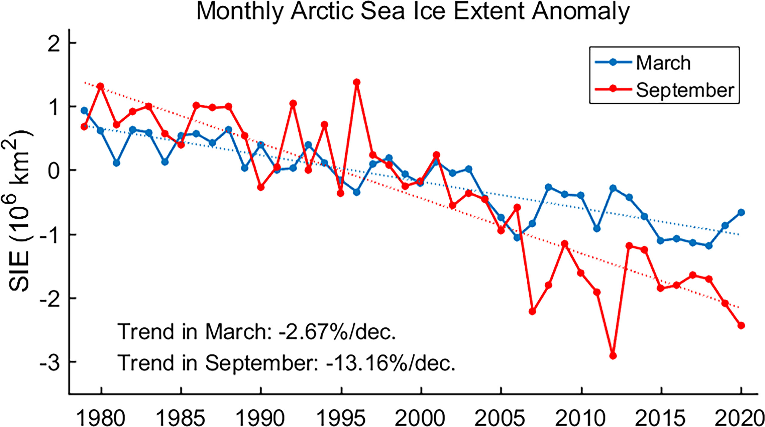
Figure 1 The monthly Arctic sea ice extent (SIE) anomaly relative to the 30-yr reference period from 1981 to 2010. Blue and red dotted lines represent the linear fitting of the extent anomaly in March and September, respectively, and the trends of SIE in the two months are also given. Data are obtained from NSIDC.

FIGURE 2

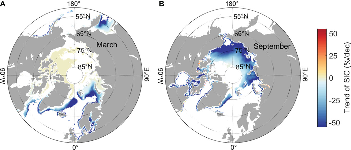
Figure 2 Multi-decadal trend of the Arctic sea ice concentration (SIC) in March (A) and September (B) during 1979–2020. Only trends that are significant at 95% confidence level based on Mann-Kendall test are shown. Data are obtained from NSIDC.

With the significant observed retreat of sea ice in recent years, socio-economic activities in the Arctic region are growing, motivating the need for accurate and timely forecasts of sea ice to serve advanced planning of shipping routes (Lee and Song, 2014; Eguíluz et al., 2016). In addition, seasonal to inter-annual sea ice prediction is valuable for managing policy responses, which are closely related to the resource development and are beneficial for coastal communities, industry stakeholders, and wildlife in the Arctic (Meier et al., 2014; Segal et al., 2020). Developing and improving sea ice forecasting methods is also a science-motivated effort to test our understanding and ability in predicting changes in the Arctic (Blanchard-Wrigglesworth et al., 2017).

Monthly to seasonal forecasts provide a long-range outlook of changes in the sea ice cover over periods of a few weeks or months. Possible predictability of Arctic sea ice in different seasons has been explored extensively in many studies. The persistence of anomalies in the initial sea ice state, as well as physical interactions between sea ice and atmospheric or oceanic conditions, provide the basis for forecasting sea ice characteristics in the Arctic (Guemas et al., 2016; Batté et al., 2020). Previous studies using global coupled models (GCMs) have provided estimates of potential seasonal to decadal sea ice prediction skill limits. For instance, Day et al. (2014) found that the memory or lagged correlations for total sea ice extent in the Arctic are around 2–5 months in GCMs, dependent on the initialization month (see their Figures 7A, 8A), which are consistent with the results of Blanchard-Wrigglesworth et al. (2011) using satellite observations. Whereas, Cruz-García et al. (2019) found that the potential predictability of sea ice volume in the Arctic may be up to three years ahead but with a significant spatial variation. Previous studies also analyzed the regional prediction skill and predictability of Arctic SIE using seasonal forecasts of dynamical prediction systems (Bushuk et al., 2019; Bushuk et al., 2022). These studies show that winter SIE can be skillfully predicted up to 11 months in advance benefit from the persistence of both SIE and upper ocean heat content, while the prediction skills of summer SIE are limited within 4 months by the Arctic springtime predictability barrier (Blanchard-Wrigglesworth et al., 2015; Bonan et al., 2019; Bushuk et al., 2020). Currently, physics-based numerical climate models are widely used to generate the Arctic sea ice forecasts at sub-seasonal and seasonal time scales (Day et al., 2014; Zampieri et al., 2018; Yang et al., 2020). However, numerical models are computationally expensive and the predictive accuracy is highly dependent on the initial conditions (Blanchard-Wrigglesworth et al., 2011). It has been found that current numerical models have little additional skill beyond persistence forecasts in sea ice prediction at lead times longer than several weeks (Blanchard-Wrigglesworth et al., 2015; Wayand et al., 2019).

Meanwhile, the data-driven artificial intelligence (AI) approaches, including machine learning and deep learning approaches, have been increasingly applied to the earth system science including climate prediction (Reichstein et al., 2019). For example, Ham et al. (2019) successfully made skillful forecasts of El Niño/Southern Oscillation with lead times up to one and a half years using a deep neural network, showing a great potential of deep learning approaches in climate prediction. Some relatively popular machine learning or deep learning methods have also been utilized in the Arctic sea ice forecasts. Regression techniques using only sea ice input or additional predictors could provide adequate sea ice predictions and have proven their ability to be competitive with the dynamical model counterparts (Gregory et al., 2020; Horvath et al., 2020). Chi and Kim (2017) proposed a prediction model using the long short-term memory network (LSTM). Their model shows better performance in the 1-month lead prediction of sea ice than a traditional statistical model, but the predictions were less accurate in the melting season. Kim et al. (2020) investigated the skill of an intelligent Arctic sea ice prediction model based on convolutional neural networks (CNNs) and found that the model is effective in sea ice prediction at 1-month lead time. Andersson et al. (2021) designed a prediction system using an ensemble of U-Net (a kind of CNN variant) networks and made skillful probabilistic Arctic sea ice forecasts on seasonal time scale. Convolutional LSTM networks have also been used to make extended range sea ice forecast. For example, Liu et al. (2021) indicated that Convolutional LSTM is able to forecast regional Arctic SIC skillfully at weekly to monthly time scales.

The formation and evolution of sea ice involves complex nonlinear processes caused by the atmosphere-sea ice-ocean interactions. Compared with traditional statistical models, deep learning methods are good at expressing non-linear relationships of variables and simulating the complex dynamical systems. In light of the previous studies, we try to develop a monthly to sub-seasonal forecast model of sea ice using LSTM networks. Compared to the previous studies on LSTM-based sea ice prediction, two improvements will be implemented in the original LSTM networks to pursue better forecasting skills: the optimization of the loss function and the introduction of an attention module. Moreover, forecasting skills on sea ice edge will also be evaluated to provide a more comprehensive assessment of the method proposed in this study. By comparing the model performance with other approaches, we will discuss the applicability and reliability of our deep learning method in Arctic sea ice prediction.

The rest of the paper is organized as follows. Section “Dataset” briefly introduces the observational data used for the building and assessments of our LSTM networks. Section “Methods” describes the structure of our LSTM networks and the evaluation methods for the forecasting skills. Detailed results analyses, including the Arctic sea ice variability in observations and the evaluation of forecasting skills of different sea ice characteristics, are shown in section “Results”. Section “Conclusions and Discussion” summarizes the results of the present study and outlines possible directions for future works on sea ice forecast in the Arctic.

2 Dataset

In this study, a satellite-based product of Arctic SIC (https://nsidc.org/data/NSIDC-0051/versions/1) (Cavalieri et al., 1996) provided by the NSIDC is used as the training data of LSTM forecasting models and as the ground truth for evaluating the models’ forecasting skills during the test period. SIC is computed from passive microwave satellite measurements of brightness temperature since 26 October 1978, using the NASA Team retrieval algorithm developed by the Oceans and Ice Branch, Laboratory for Hydrospheric Processes at NASA Goddard Space Flight Center (GSFC). The brightness temperature is observed from different sensors, including the Nimbus-7 Scanning Multichannel Microwave Radiometer (SMMR), the Defense Meteorological Satellite Program (DMSP) -F8, -F11 and -F13 Special Sensor Microwave/Imagers (SSM/Is) and the DMSP-F17 Special Sensor Microwave Imager/Sounder (SSMIS). The dataset of SIC is provided on a Lambert azimuthal equal area projection with a nominal spatial resolution of 25 km × 25 km. In total, there are 304 × 448 data points in each month. The spatial domain focused in this study is the Arctic region covered by the satellite-based observation (about 31–90°N, 180°W–180°E). Considering the higher uncertainties of observation in late 1978, we only use SIC data with the temporal coverage of 42 years between 1979 and 2020.

In this study, the large sea ice dataset from NSIDC is employed to train our deep neural networks and then to predict Arctic SIC, without incorporating any other physical parameters to ensure a relatively fast computing speed. Before fitting SIC data into LSTM models, non-sea ice grid points, including points of land, open ocean, and lake ice, are removed. In addition, points in the “pole hole” (the region around the pole not imaged by the sensor) are set to fully ice-covered, i.e., SIC equals 100% on these points. Forecasting skills are evaluated for both SIC and SIE; the latter is defined as the area of ocean with at least 15% SIC.

3 Methods

3.1 Predictability of Arctic Sea Ice

Using anomaly correlation coefficients (ACCs) for different target months at different lead times (Figure 3), we examine the persistence of pan-Arctic SIC and total SIE based on the satellite observations during 1979–2020. Persistence of SIC is represented as the regional averaged ACC for SIC on all grid points. It is obvious that the persistence is much longer in September, October, and March, for both the ice concentration and the extent. In contrast, low correlations exist between successive months in the transition season (e.g., May and June) when sea ice is rapidly growing or melting. In this study, we mainly focus on the sea ice situation in summer and early autumn.

FIGURE 3

Figure 3 Persistence of the Arctic SIC (A) and total SIE (B) based on the anomaly correlation coefficients (ACCs) of monthly SIC and SIE in January to December at different lead times. Note that ACCs in (A) are the regional averaged values for SIC on all grid points. Data of SIC and the calculated SIE during 1979–2020 are from NSIDC.

Sea ice in September and October is highly correlated with sea ice in the previous 1–3 months, and thus months from June to August show predictive skills in forecasting late summer sea ice. As pointed out by Andersson et al. (2021), the precondition of the sea ice pack is a key predictor, with persistence of sea ice anomalies potentially lasting at seasonal timescales, especially for the ice in late summer. In addition, correlations are extremely low for sea ice between summer and spring for the same year. The weak correlation may be a manifestation of the springtime predictability barrier.

The above-mentioned possible sources of sea ice predictability, including the seasonal cycle, the multi-decadal trend, and the persistence of sea ice anomalies (especially in summer months), are essential for our data-driven forecasting approaches used in this study.

3.2 Long Short-Term Memory Networks

LSTMs is a special type of Recurrent Neural Networks (RNNs) introduced by Hochreiter and Schmidhuber in 1997 (Hochreiter and Schmidhuber, 1997). Like RNNs, LSTMs are networks in the form of a chain of repeating modules, allowing information to persist, so that they are generally used to deal with time series problems. However, when training a classic RNN using back-propagation, the long-term gradients can “vanish” or “explode”, because the computations involved in the process use finite-precision numbers. LSTMs could partially solve the vanishing gradient problem, because LSTM modules or units allow gradients to also flow unchanged, making LSTM capable of handling long-term dependencies (Calin, 2020).

Generally, a single LSTM cell contains four interacting neural network layers acting as four activation functions [three sigmoid (σ) and one hyperbolic tangent (tanh) functions], which are marked by yellow boxes in Figure 4B. This kind of module structure is more complex than that in RNNs, which contains only one layer of tanh. LSTM controls the transfer and loss of information by a memory cell state (the straight black line at the top of Figure 4B) and three “gates” (marked by red dashed boxes in Figure 4B). The cell state is responsible for remembering the previous state while the gates are responsible for controlling the amount of memory to be exposed.

FIGURE 4

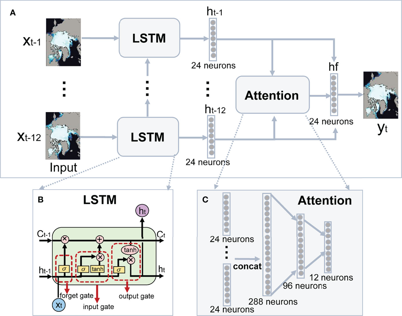
Figure 4 The overall architecture of the attention-based LSTM with combination loss (A) and the details of a single LSTM cell (B) and the attention module (C). In (A), “x” is the input SIC, “y” is the forecasted SIC, “h” denotes hidden state of LSTM, “hf” is the final hidden state processed by the attention module. In (C), “concat” represents the concatenating of all the hidden states together.

Chattopadhyay et al. (2020) have found that deep neural networks including LSTM are able to reproduce both the short-term evolution and the long-term statistics of dynamical systems, which provides a basis for this study to extract the nonlinear relations of sea ice time series and to make sea ice forecasts based on observational data. In contrast to the traditional statistical methods, the nonlinearity introduced by LSTM could effectively contribute to the skill of the sea ice forecast. Based on the finding of Chi and Kim (2017), we use the observed SIC in the preceding 12 months {x_t-12, x_t-1} as the input data to make 1-month lead forecast at each grid point. These data are fed into LSTM one by one, and the final hidden state h_t-1 at the last month is used to predict y_t via a fully-connected operator. The whole network is trained by the widely used loss function based on the mean squared error (MSE) between the predicted y_t and observed SIC x_t, which can be described as $\frac{1}{n}{\displaystyle {\sum }_{i=1}^n{\left(x^{\left(i\right)}-y^{\left(i\right)}\right)}^2}$ Then, we keep the network structure unchanged, and only add the mean absolute error (MAE) into the original loss function, resulting in a combined loss function of MSE and MAE, i.e., $\frac{1}{n}{\displaystyle {\sum }_{i=1}^n{\left(x^{\left(i\right)}-y^{\left(i\right)}\right)}^2+\left|x^{\left(i\right)}-y^{\left(i\right)}\right|}$ Such a loss function could effectively reduce the impacts of outliers, thus expecting to achieve better predictions. Using this loss function, we finally develop an improved LSTM model.

As shown in Figure 4, our final model incorporates an attention module into the original LSTM network. Different from the traditional LSTM models which only consider the contribution of the last hidden state h_t-1 to the final prediction, the attention module is able to deal with all of the hidden states {h_t-12, h_t-1} in the preceding 12 months, and automatically recognize the importance of them. To achieve this goal, we construct the module by two fully-connected layers, and the last one outputs the importance of the weights {w_t-12, w_t-1} for 12 months. After that, the hidden states are multiplied by the corresponding weights to get the final hidden value, which can be formulated as $hf={\displaystyle {\sum }_{i=1}^{12}\left[w_{t-i}\times h_{t-i}\right]}$ Same as traditional LSTM models, hf is finally fed into a fully-connected layer to get y_t. In addition, during the training phase, we employ a combination loss of MSE and MAE to better optimize the proposed network. For LSTM in the network, there is 1 hidden layer with 24 neurons. For the attention module, the number of neurons in the first and the second fully connected layer is 96 and 12, respectively. We choose Adam as the optimizer to optimizing the weights. The learning rate and the batch size are set to 0.001 and 128, respectively. For simplicity, the three forecasting models are abbreviated as LSTM_MSE (original LSTM with MSE-based loss function), LSTM_MAE (LSTM with MSE and MAE combined loss function), and LSTM_Attention (attention-based LSTM with MSE and MAE combined loss function), respectively.

For sea ice forecast at longer lead times (2–6 months), we use a recursive approach. The predicted values at shorter lead time are treated as new inputs into the same forecasting model to make predictions at longer lead time. Take the forecast of September 2019 SIC as an example. For the 1-month lead time forecast, SIC observation from September 2018 to August 2019 is used as inputs to LSTM network. Then to generate a 2-month lead time forecast, we use SIC observation from September 2018 to July 2019 and SIC forecast of August 2019 as inputs. Monthly SIC of the passive microwave observations (see the section “Datasets”) from 1979 to 2014 (36 years, 432 months) are used to construct the training set for LSTM network, while data from 2015 to 2020 (6 years, 72 months) are used to construct the test set to verify the skills of the prediction models. To generate the training set, the 432-month data needs to be divided into input-output data pairs. The input consists of preceding 12-month data, while the output is the subsequent 1-month data. At each month, all of the grid points could be used. Thus, more than 10 million of training samples were generated to train the proposed model. Similar methods are used to the 72-month test data, and more than 3 million of test samples were produced. The LSTM related models are implemented on a personal computer with an Intel core i7-4790, 3.60-GHz processor, 32-GB RAM, and a GTX TITAN X graphic card. The training time for LSTM_MSE, LSTM_MAE, and LSTM_Attention are 69.07, 69.08, and 69.31 minutes, respectively, while the testing time for them are 0.90, 0.91, and 1.21 seconds, respectively.

3.3 Benchmark Models: Empirical and Numerical Models

Referring to the work of Liu et al. (2021), we also assess our LSTM mos against two empirical benchmark models using sea ice persistence and climatology. The persistence is defined as the SIC anomaly at lead time step 0 added to the SIC climatology of the target forecast month, while the climatology of SIC in each month is defined as the average of SIC in a 10-yr sliding window preceding the respective forecast target time. For example, the 1-month lead persistence forecast of SIC in September 2019 is the anomaly of August 2019 plus the climatology of September SIC in 2009–2018.

To compare LSTM with numerical model-based forecasts, sea ice prediction results from two numerical climate models are also analyzed. Previous studies have indicated that the numerical systems from the European Centre for Medium-Range Weather Forecasts (ECMWF) and the U.K. Met Office (UKMO) provide the state-of-the-art Arctic sea ice prediction skills (Zampieri et al., 2018; Wayand et al., 2019). In this study, the seasonal ensemble forecast products from these two systems are compared with forecasts of our deep learning methods. The two model systems (hereafter, abbreviated as ECMWF-C3S and UKMO-C3S) are contributing to the Copernicus Climate Change Service (C3S). The dataset includes forecasts created in real-time (since 2017) and retrospective forecasts (hindcasts) from 1993 to 2016. The brief information of these two models is given in Table 1. These models are chosen because of their time range (January 2015–December 2020 for ECMWF, and January 2015–December 2016 for UKMO) available for the intercomparing in this study and the popularity of their sea ice models. Forecasts of SIC from the two models are re-gridded from their latitude-longitude grid to the NSIDC equal area grid using bilinear interpolation method. The interpolation is performed after converting the latitude-longitude coordinate to distance coordinate.

TABLE 1

Table 1 Brief information of the two C3S models.

3.4 Evaluation Metrics

This study evaluates the forecasting model performance based on the standard deterministic accuracy metrics: the root-mean-square error (RMSE), mean absolute error (MAE) and anomaly correlation. Taking the evaluation of SIC prediction as example, the RMSE and MAE of SIC are defined in formulae (1) and (2). $SI{C}_i^f$ is the forecasted value of SIC, $SI{C}_i^o$ is the observed SIC, and N is the total number of grid points. The errors are spatially averaged after masking the land, open ocean, and the observational “pole hole” grids.

$\begin{array}{ll}RMSE=\sqrt{\frac{1}{N}{\displaystyle {\sum }_{i=1}^N{\left(SI{C}_i^f-SI{C}_i^o\right)}^2}}& (1)\end{array}$

$\begin{array}{ll}MAE=\frac{1}{N}{\displaystyle {\sum }_{i=1}^N\left|SI{C}_i^f-SI{C}_i^o\right|}& (2)\end{array}$

In addition, the assessment of the skills in predicting the Arctic sea ice edge is based on the Integrated Ice Edge Error (IIEE, Goessling et al., 2016). The IIEE is defined as the sum of ocean areas where the presence of sea ice (defined with a 15% SIC threshold) is overestimated and underestimated with respect to the observations. In other words, this verification metric describes the area where the forecasts and observations disagree on the presence of sea ice with concentration being above or below 15%. In this study, the two components of IIEE, i.e., the overestimated error and underestimated error of sea ice edge, are abbreviated as OE and UE for simplicity.

$\begin{array}{ll}IIEE=OE+UE& (3)\end{array}$

$\begin{array}{ll}OE={\displaystyle {\int }_A\text{max}\left(c_f-c_o,0\right)dA}& (4)\end{array}$

$\begin{array}{ll}UE={\displaystyle {\int }_A\text{max}\left(c_o-c_f,0\right)dA}& (5)\end{array}$

where c=0 when the SIC is higher than 15% and c=1 when SIC is less than 15%. The subscripts f and o denote the forecast and observation. A denotes the area of interest.

The IIEE has been widely used in previous studies focusing on the sea ice forecast (e.g., Blockley and Peterson, 2018; Roach et al., 2018; Allard et al., 2020; Batté et al., 2020; Liu et al., 2021). By taking into account possible error compensations between the overestimation and underestimation of the presence of sea ice, the IIEE could present a better estimate of the ability of forecast models to predict SIC in different Arctic basins.

It is noteworthy that only the mean forecast results of the dynamical models are concentrated on in this study, thus the evaluation metrics used here are relatively simple and can only partly reflect the skills of the forecasting model. Besides, considering that the reliability of a forecast model comes from its ensemble forecasts while our preliminary LSTM-based approach has no ensemble component at present, this approach used here is not yet able to report on the reliability of the sea ice forecast.

4 Results

4.1 Forecasting Skills of Pan-Arctic Sea Ice Extent

At first, we evaluate the hindcast or re-forecast skills of LSTM models for pan-Arctic SIE derived from SIC forecasts at 1-month lead time. We examine the month-to-month and inter-annual variability of the predicted pan-Arctic SIE during January 2015–December 2020. Figure 5 shows the monthly SIE anomaly obtained by three LSTM models and three benchmark models (ECMWF-C3S, Climatology, and Persistence), as well as the absolute errors of their SIE forecasts compared to the satellite observation. When calculating the anomaly, the common reference period is the 30-yr climatology from 1981 to 2010, which is also used in this study. In general, all the forecasts from three LSTM models are consistent with observation in the seasonal variations of SIE anomaly. Greater anomaly occurs in summer to early autumn compared to the rest of the year (Figure 5A). Obviously, LSTM_Attention and LSTM_MAE perform better than LSTM_MSE in reproducing the extreme low SIEs in October of 2016, 2019, and 2020. Monthly SIE anomaly from LSTM_Attention forecast shows a significant positive correlation with observation during our test period 2015–2020, with the correlation coefficient reaching about 0.8. The absolute errors of SIE between LSTM forecasts and observation (Figure 5B) also show that, in most time of the test period, predicted SIEs from LSTM_Attention and LSTM_MAE are closer to the observation compared to that from LSTM_MSE. This result confirms that the optimization of the deep learning network could improve the forecasting skills by considering previous sea ice conditions as much as possible. It is nevertheless noteworthy that all the three models predict a false minimum SIE in October 2017. This loss of skill reflects the dependence of deep learning-based forecasts on the training data, or their weak capacity reflecting the impacts from strong, synoptic-scale processes on sea ice development.

FIGURE 5

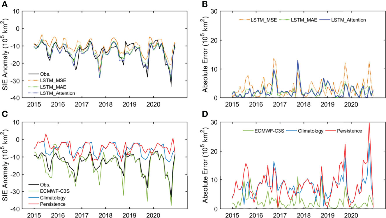
Figure 5 Monthly Arctic SIE anomaly predicted by three LSTM models during January 2015–December 2020, with the satellite observation as a reference (A). Absolute errors of monthly SIE between forecasts from three LSTM models and the observation (B). (C, D) are similar to (A, B), but for sea ice forecasts from ECMWF-C3S, Climatology, and Persistence.

In comparison, forecast from ECMWF-C3S demonstrates slightly higher absolute error against observation (Figures 5C, D). During the test period of 2015–2020, mean absolute errors of monthly SIE are 0.23 and 0.25 million km² for LSTM_Attention and ECMWF-C3S, respectively. Consistent with LSTM_Attention, ECMWF-C3S also underestimates total Arctic SIE significantly in October 2017, which is quite interesting and worthy of further study. The two empirical models of Climatology and Persistence show much higher SIE errors compared to forecasts from other methods.

For long-term (i.e., the test period of 2015–2020) averaged SIE in different months among the year, LSTM_Attention demonstrates higher skill than LSTM_MSE and LSTM_MAE in most months of the year. The RMSE and MAE (Figure 6A) of forecasted SIE are the largest in early autumn (October to November). The relatively low skill is probably due to the higher sea ice mobility and thus the larger uncertainty of forecasted ice edge location during this season of year. This is also a common characteristic for sea ice forecasts from the dynamical model ECMWF-C3S and two empirical benchmark models (Figure 6B). Except for February and July, LSTM_Attention shows comparable RMSE and MAE with ECMWF-C3S, especially in late summer and early autumn. Combined with their absolute errors in Figure 5, this result suggests that LSTM_Attention is comparable to dynamical models in predicting ice extent, especially in the season when marine operations peak.

FIGURE 6

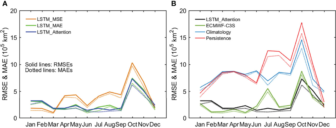
Figure 6 RMSEs (solid lines) and MAEs (dotted lines) of forecasted monthly SIE in 2015–2020 using three LSTM models (A) and using LSTM_Attention, ECMWF-C3S, and two empirical models (B). In both (A, B), the lead time is one month.

Since 2008, the Sea Ice Outlook (SIO) initiative (Stroeve et al., 2014), which is now under the auspices of the Sea Ice Prediction Network (SIPN, http://www.arcus.org/sipn/sea-ice-outlook), has collected several sources of seasonal forecasts (statistical, dynamical and heuristic) for the September pan-Arctic SIE at up to three month lead times. To further evaluate the skill of LSTM_Attention, we compare our results with the SIO median and the best SIO estimates for the 2015–2020 September SIE as shown in Table 2. The SIO forecasts are based on the August reports (i.e., with 1-month lead time) submitted by all the contributors each year. Although showing overestimation and underestimation of SIE in the first two years, the prediction of LSTM_Attention is slightly closer to the observations than the SIO median since 2017; this demonstrates the potential of deep learning approaches in operational monthly to sub-seasonal sea ice forecasting. Meanwhile, there is still a gap between LSTM_Attention forecasts and the best SIO approaches, indicating that more work is needed to improve the skills of our LSTM-based method.

TABLE 2

Table 2 Values of the observations, the SIO contributions (August report of SIO median and the best SIO forecast), and the LSTM_Attention 1-month lead forecast for September monthly mean pan-Arctic SIE in the year 2015–2020 (unit: 10⁶ km²).

4.2 Forecasting Skills of Sea Ice Concentration

To explore the possible explanations of SIE forecasting skills from LSTM models, we examined the performance of LSTM_Attention in representing the spatial distribution of sea ice cover. Examples of the September SIC forecasts from attention-based LSTM at 1-month lead time are shown in Figures 7, 8. We examine the extreme years with record minimum September SIE, including 2015, 2016, 2019, and 2020 (the second-lowest ice extent on record). Prediction results from the UKMO-C3S are only available in 2015 and 2016 during our test period, and thus the inter-comparisons including this model are performed only in these years.

FIGURE 7

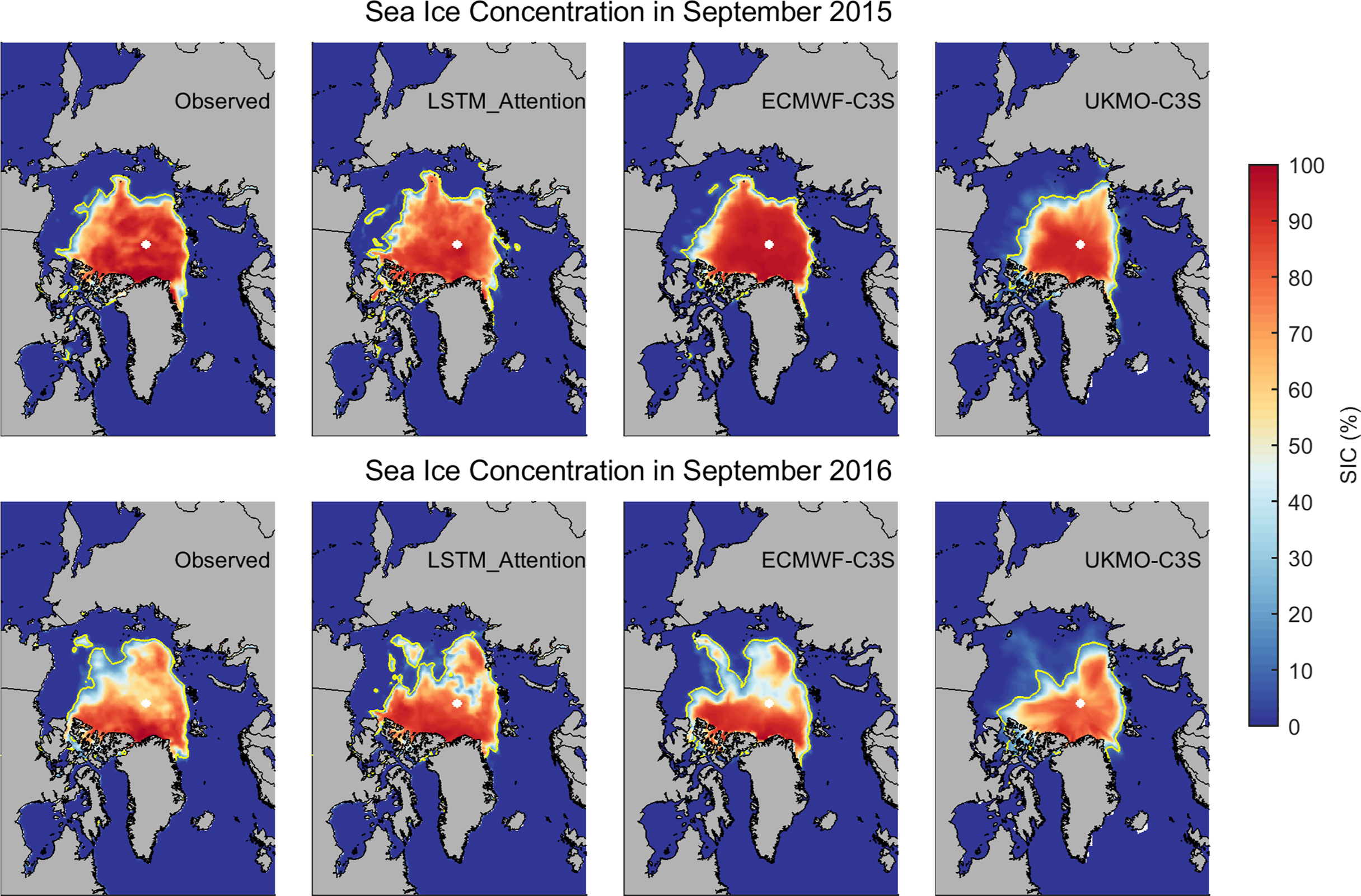
Figure 7 Observed and predicted Arctic SIC by LSTM_Attention, ECMWF-C3S and UKMO-C3S in September 2015 (upper panel) and September 2016 (lower panel). The yellow line in each subplot represents the observed or predicted ice edge for that month.

FIGURE 8

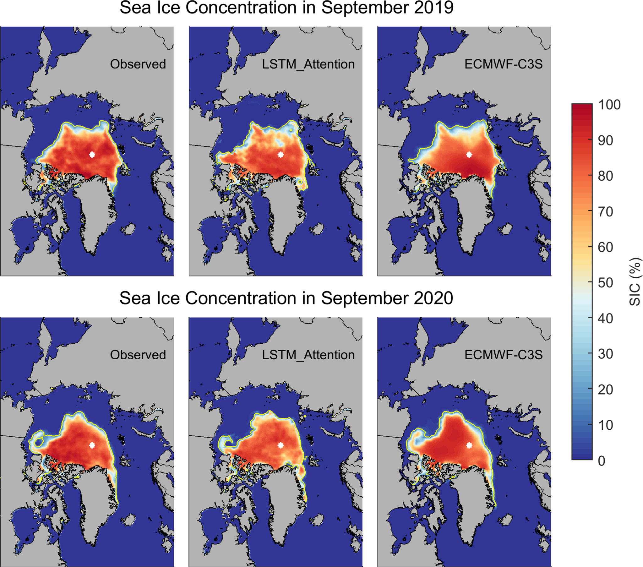
Figure 8 Observed SIC and predicted SIC by LSTM_Attention, and ECMWF-C3S in September 2019 (upper panel) and September 2020 (lower panel). The yellow line in each subplot represents the observed or predicted ice edge for that month.

As shown in Figures 7, 8, the attention-based LSTM successfully reproduces the spatial pattern or the regional variation of summer sea ice cover in extreme years that recorded unforeseen SIE minimums. In the first two years, LSTM_Attention outperforms UKMO-C3S and is comparable to ECMWF-C3S in predicting the location of sea ice edge. Yet, in September 2016, the concentration underestimation in central Arctic from LSTM_Attention is obvious and is probably the cause of total SIE underestimation in this September.

The spatial distribution of year-round mean MAE of ice concentration in January 2015–December 2020 forecasted by LSTM_Attention is shown in Figure 9. For all 12 months, concentration errors are the largest in marginal ice zones. Physically, marginal ice zones are characterized by extremely active ice motions and air-sea-ice interactions (e.g., Zippel and Thomson, 2016; Boutin et al., 2020), making it more challenging for sea ice prediction. For the whole Arctic, RMSE of ice concentration forecasted by LSTM_Attention is lower than the two empirical models and ECMWF-C3S in each month (Figure 10B). Also shown in Figure 10B is that RMSE of forecasted SIC from LSTM_Attention is relatively low in late summer (August and September) but higher in October, similar to the situation of pan-Arctic SIE (Figure 6B). ECMWF-C3S also has higher forecasting skill than persistence during this time, but it does not outperform the 10-yr climatology forecast.

FIGURE 9

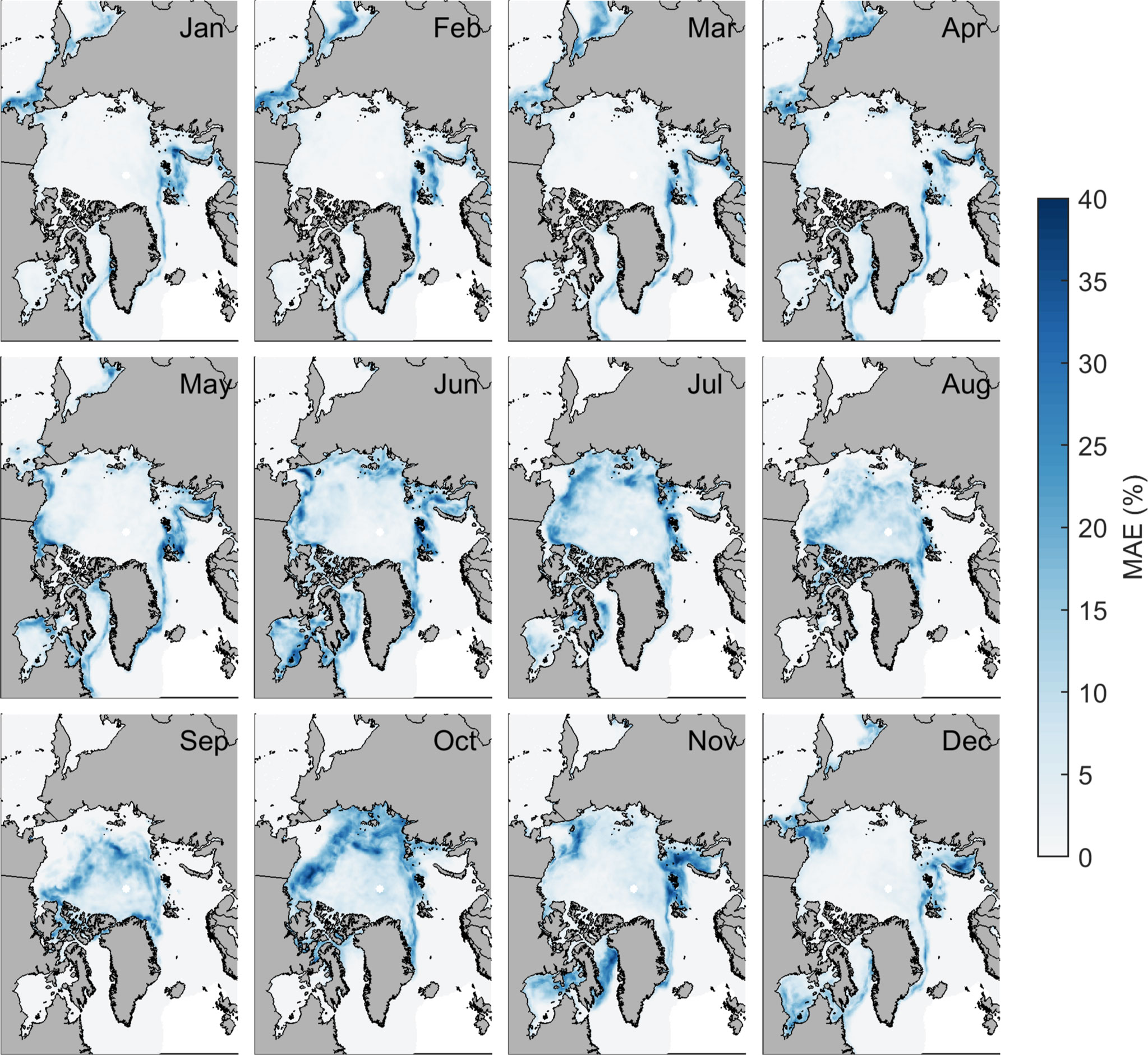
Figure 9 Mean MAE of LSTM_Attention forecasted SIC in January 2015–December 2020 at 1-month lead time.

FIGURE 10

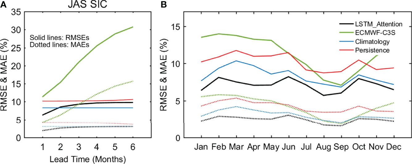
Figure 10 Averaged RMSEs (solid lines) and MAEs (dotted lines) in 2015–2020 of the July–August–September (JAS) SIC forecasts at lead times of 1 month to 6 months (A) and averaged RMSEs and MAEs in 2015–2020 of monthly SIC forecasts at 1-month lead time (B) using LSTM_Attention, ECMWF-C3S, climatology, and persistence.

We also show the July-August-September (JAS) RMSE of lead-time-dependent SIC forecasts by different approaches (Figure 10A) to examine the sea ice predictive skills of LSTM_Attention. In general, RMSE increases with the increased lead time except for the climatology forecast. LSTM_Attention outperforms both the persistence and the ECMWF-C3S forecast for lead times from 1 month to 6 months. In particular, the RMSE over time of SIC from LSTM_Attention is lower than the persistence with lead times up to 2 months, providing the basis for its skill in total ice extent prediction. At lead time of 2 months, the skill of LSTM_Attention is comparable to the climatology and thus it is vanished.

The above-mentioned assessments confirmed the potential of LSTM_Attention to predict summer concentration fields. In practice, it is important to know whether a region is ice free or not for the increasingly frequent shipping and related activities in the Arctic Ocean. The Integrated Ice Edge Error (IIEE), which is first introduced by Goessling et al. (2016), has been proved to be an appropriate objective metric. This metric could well evaluate the model’s forecasting skill in the position of the ice edge (with the concentration threshold of 15%) and will be analyzed in the following section.

4.3 Forecasting Skills of Sea Ice Edge

Figure 11 shows the monthly IIEE and its two components, OE and UE, during the test period 2015–2020 from the three LSTM models. Similar to the absolute error in total ice extent (recall Figure 5B), IIEE of LSTM_Attention is much lower than LSTM_MSE and LSTM_MAE. The seasonal cycle (Figure 12) of IIEE shows that the forecasting ice edge error is relatively larger in early autumn (October) than in other months, which is consistent with LSTM_Attention’s low skill in forecasting October ice extent (recall Figure 6). Figure 10 also demonstrates that the improvement of IIEE from the attention-based LSTM is mainly contributed by the decrease of OE in the forecast fields of LSTM_Attention. As for the UE in LSTM_Attention forecast, it gets worse instead of better compared to the previous approaches (Figure 11C). Future effort is warranted to explain and reduce this underestimated component of IIEE in LSTM model.

FIGURE 11

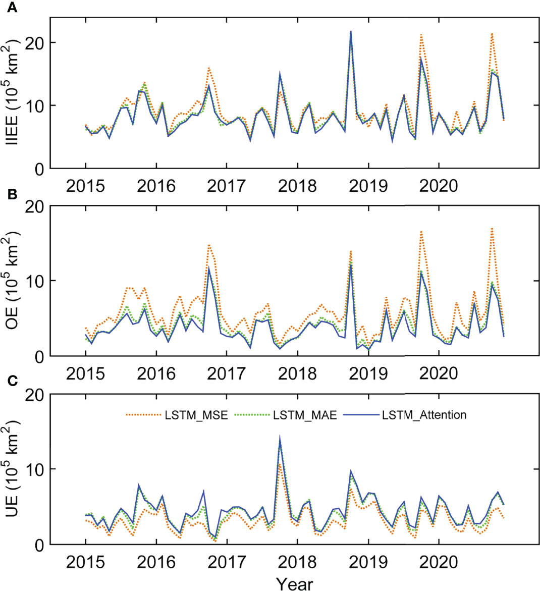
Figure 11 Monthly Integrated Ice Edge Error (IIEE) (A), overestimated (B) and underestimated (C) ice edge error of the three LSTM-based forecasting models for the test period 2015–2020.

FIGURE 12

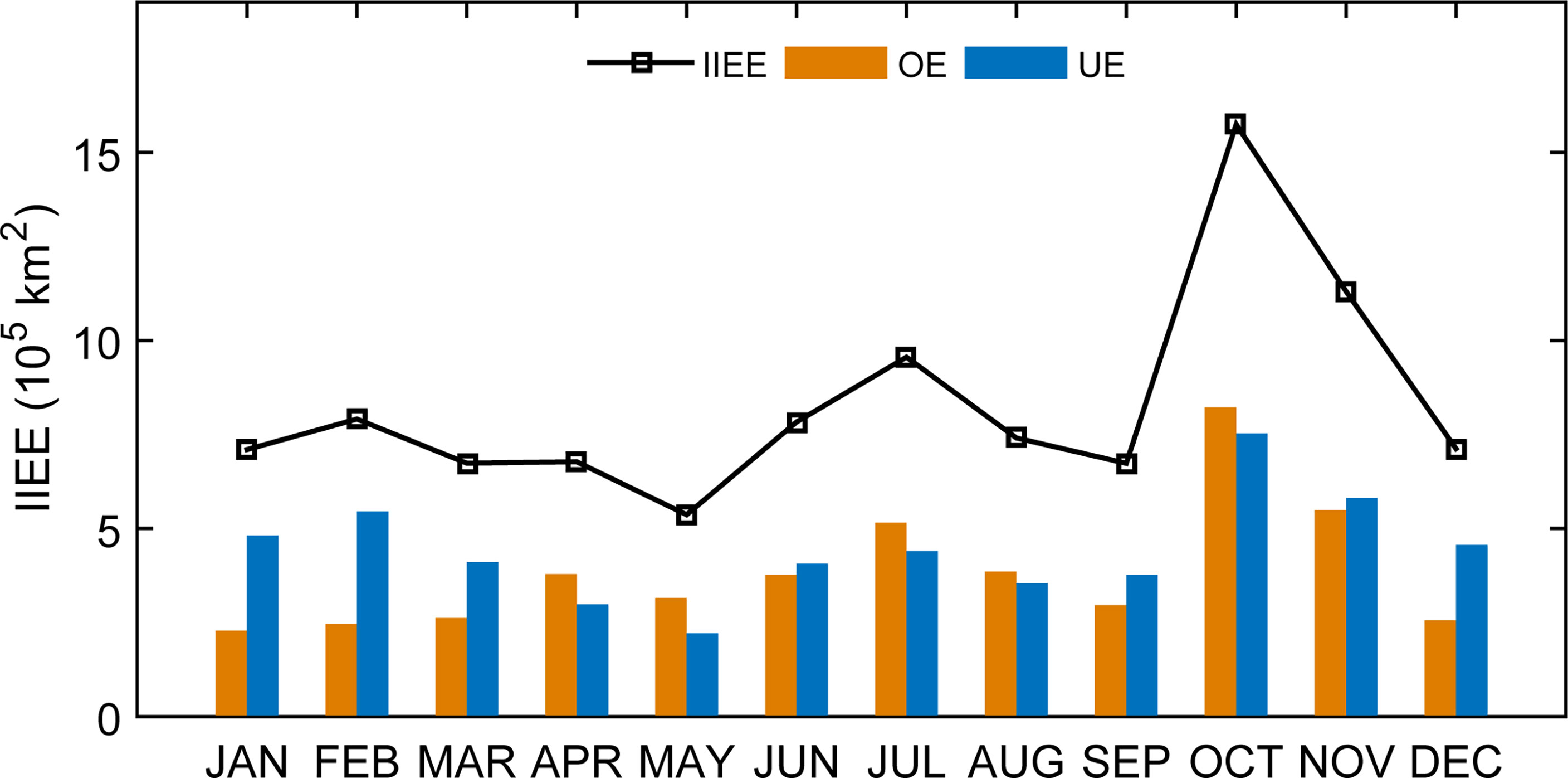
Figure 12 Seasonal cycle of IIEE and its two components, overestimated error (OE) and underestimated error (UE), during the test period 2015–2020 from sea ice forecast of LSTM_Attention.

The extremely high IIEE and its two components in October and November (Figure 12) is associated with the high MAE of total ice extent forecasted by LSTM_Attention (Figure 6A). Moreover, the discrepancy between IIEE and MAE also highlights the limitations of conventional metric for ice extent evaluations like MAE: the IIEE contains the “misplacement error”, reflecting too much ice in one area and too little in another, which is not included in MAE of the total ice extent.

Figure 13 shows the IIEEs of summer (July–August–September, JAS) sea ice forecasts over 2015-2016 versus lead time. Forecasts are from LSTM_Attention and the two C3S dynamical models, respectively. It is not surprising that the IIEE increases with the increasing lead time. LSTM_Attention is comparable to ECMWF-C3S and UKMO-C3S in 1-month lead time forecast, while it outperforms the two dynamical models at lead time of 2 months. IIEEs of forecasts from LSTM_Attention and ECMWF-C3S in 2015–2020 are similar to those for 2015–2016 and thus are not shown here. Besides, LSTM_Attention obviously differs from the dynamical models in the allocation of the two components OE and UE. LSTM_Attention forecast provides comparable amounts of OE and UE, while in the two dynamical models’ forecasts, UE dominants the total IIEE error.

FIGURE 13

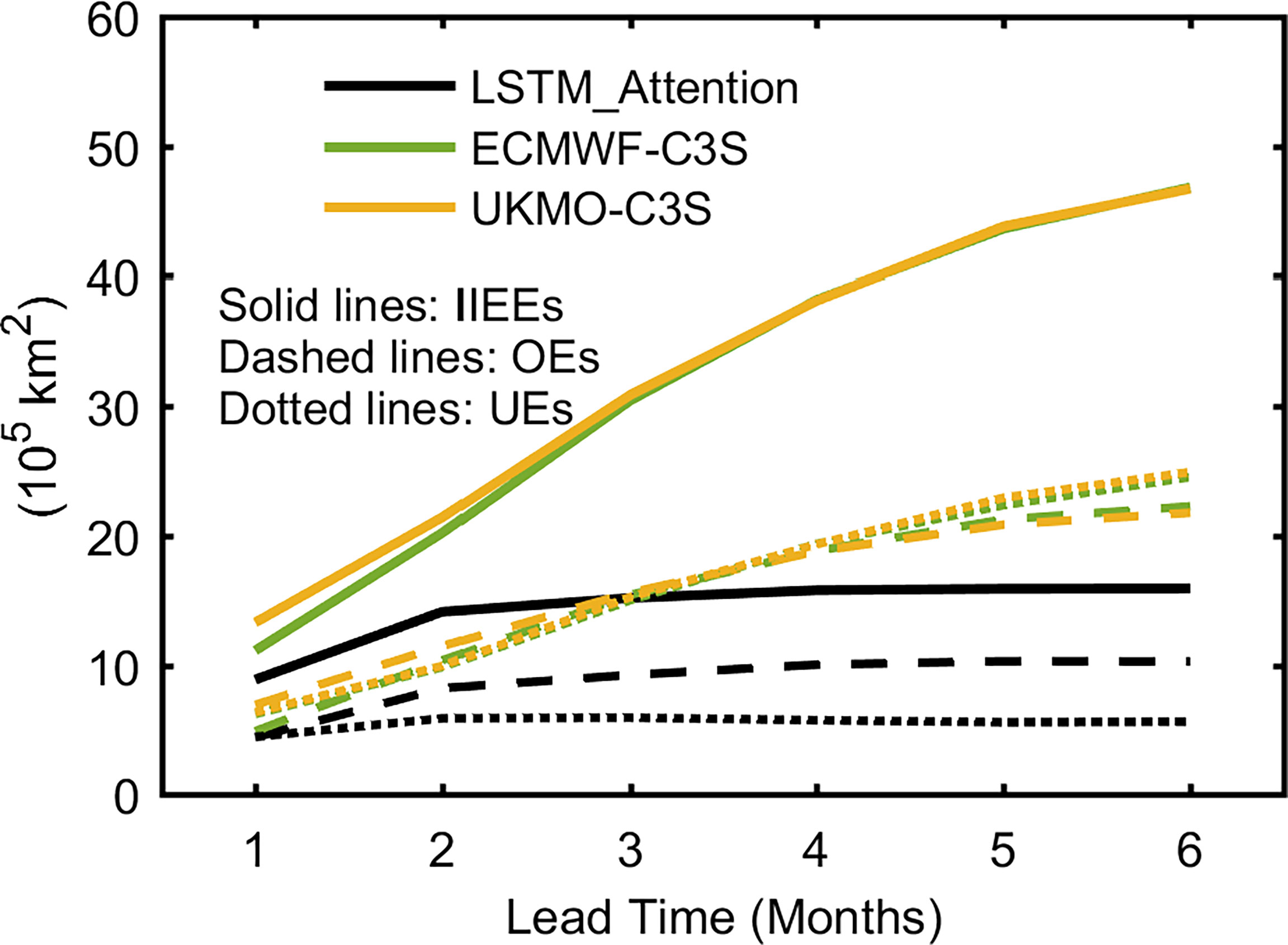
Figure 13 Averaged IIEEs (solid lines), OEs (dashed lines), and UEs (dotted lines) in 2015–2016 of the July–August–September (JAS) sea ice forecasts at lead times of 1 month to 6 months using LSTM_Attention, ECMWF-C3S, and UKMO-C3S.

We take September 2016 as an example to examine the spatial structures of the gridded two components of IIEE (Figure 14). For all the three forecast fields, the overestimated and underestimated error components are mainly located in the Pacific sector of the Arctic Ocean. One possible reason is that sea ice in the Atlantic sector (including the Kara Sea and Barents Sea) has almost completely melted in September, pushing the ice edge northward to the central Arctic Ocean. The larger ice edge error in the Pacific sector reflects the great inter-annual variation of sea ice cover due to strong advection and melting processes in this region (e.g., Bi et al., 2019). Actually, in addition to the most obvious decreasing trend (Figure 2B) since 1979, September ice concentration in the Pacific sector also shows the largest inter-annual variation in contrast to other Arctic regions (figure not shown).

FIGURE 14

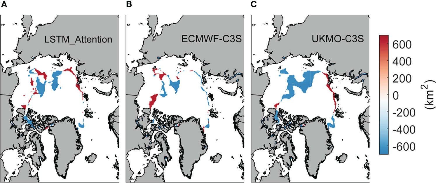
Figure 14 The spatial structure of gridded OE (red area) and UE (blue area) of sea ice forecast in September 2016 using LSTM_Attention (A), ECMWF-C3S (B), and UKMO-C3S (C), respectively, at 1-month lead time. Note that the sign of UE has been reversed from positive to negative for convenience.

Compared to UKMO-C3S, LSTM_Attention and ECMWF-C3S mainly capture the observed sea ice edge especially in the Atlantic sector, indicating that our improved LSTM network is reliable in monthly to sub-seasonal Arctic sea ice edge forecast in the melting season. This confirms the potential of our LSTM network in providing a monthly to sub-seasonal outlook of ice edge changes, which could help planning the routes in the Arctic Ocean 1 to 1.5 months in advance.

5 Conclusions and Discussion

In this study, we propose an improved Long short-term memory network (LSTM) for the monthly to sub-seasonal forecast of pan-Arctic sea ice concentration (SIC). Two improvements are implemented in the original LSTM neural network: first, the mean absolute error (MAE) is added to the traditional loss function using mean square error (MSE) to reduce the impacts of outliers in the data; second, an attention module is used to fully extract the linkage between sea ice in the target month and those in the preceding 12 months. Forecasts from the attention-based LSTM with improved loss function (LSTM_Attention) are evaluated and compared with forecasts from four benchmark models, including two empirical models (climatology and persistence) and two dynamical model systems provided by the Copernicus Climate Change Service (C3S) (ECMWF-C3S and UKMO-C3S).

With lead time of 1 months, the proposed LSTM_Attention model outperforms the persistence-based and climatology-based empirical models for summer (JAS) sea ice forecasts. LSTM_Attention is comparable to the climatology for the 2-month lead forecast but does not beat it, indicating that its forecasting skill is lost at 2-month lead. Forecasting results of LSTM_Attention are comparable to those obtained with ECMWF-C3S and UKMO-C3S, indicating that our LSTM-based method provides a good alternative to the computational expensive large models. By taking local ice concentration variations into consideration, LSTM_Attention successfully reproduces observed spatial distribution of the Arctic SIC as well as the position of the sea ice edge. The derived monthly sea ice extent (SIE) anomaly from the 1-month lead SIC forecast of LSTM_Attention shows high correlation (0.8) with observation during our test period 2015–2020. The 1-month lead September SIE forecast is slightly closer to observation than the Sea Ice Outlook (SIO) median since 2017, although large gap still exists between our LSTM forecasts and the best SIO approaches. Those results demonstrate the potential of our deep learning method in operational pan-Arctic sea ice forecasting.

We show that our data-driven LSTM model demonstrates comparable forecasting skills with two state-of-the-art dynamical models in monthly to sub-seasonal forecasts of pan-Arctic sea ice, particularly for summers with extreme sea ice retreat. However, large errors of ice concentration and ice edge still exist in the marginal seas and in the early autumn. Particularly, more attention should be paid to the low predictive capacity in LSTM models for October sea ice. Considering the complex ice-ocean and ice-atmosphere interactions, ice and non-ice variables related to these processes and the surface energy budget should be introduced as predictors into neural networks to produce more accurate forecasts. As suggested by Batté et al. (2020), combining single-model forecasts into a multi-model ensemble may bridge the gap between potential and actual forecasting skill. More importantly, when building the neural networks of LSTM in this study, we only take the sea ice variation itself into consideration to speed up the calculation. Thus, active physical processes related to sea ice development in ice-ocean boundary areas and in the transition seasons have been neglected. Besides, the predictability and prediction skill of sea ice in the Arctic may also vary depending on the region of interest (e.g., Germe et al., 2014; Bushuk et al., 2017).

In addition, it’s worth noting that since only the mean forecast results of the dynamical models are concentrated on in this study, the currently used evaluation metrics are relatively simple and can only partly reflect the skills of our forecast model. To provide comprehensive assessments, ensemble forecast results from both dynamical models and statistical deep learning models are needed to be analyzed in the future.

Based on the aforementioned issues, the undergoing work includes the building of an ensemble forecast framework consisting of different neural networks like LSTM and Convolutional Neural Network (CNN), or the combination of both LSTM and CNN, to allow for probabilistic sea ice forecasts. CNNs are suitable for mining spatial correlation in data or images, and thus could improve the forecasts on spatial distribution of Arctic sea ice cover, especially in marginal ice zones. Oceanic and atmospheric variables influencing the surface energy budget and the sea ice drift motion will be selected as predictors. Building different deep neural networks in different sub-regions of the Arctic is also necessary to reflect various dominant processes associated with regional sea ice changes in the Arctic. These warrant future studies.

Data Availability Statement

The original contributions presented in the study are included in the article/supplementary material. Further inquiries can be directed to the corresponding author.

Author Contributions

JW and RH designed and performed the experiments. JW collected and analyzed the data, and wrote the manuscript. J-JL and RH revised the manuscript. All authors contributed to the article and approved the submitted version.

Funding

This work was supported by National Key R&D Program of China (Grant No. 2020YFA0608004), the National Natural Science Foundation of China (Grant No. 42030605 and 42088101), the fellowship of China Postdoctoral Science Foundation (No. 2020M681661), and the Jiangsu Postdoctoral Research Funding Program (No. 2021K299B).

Conflict of Interest

The authors declare that the research was conducted in the absence of any commercial or financial relationships that could be construed as a potential conflict of interest.

Publisher’s Note

All claims expressed in this article are solely those of the authors and do not necessarily represent those of their affiliated organizations, or those of the publisher, the editors and the reviewers. Any product that may be evaluated in this article, or claim that may be made by its manufacturer, is not guaranteed or endorsed by the publisher.

References

Allard R., Metzger E. J., Barton N., Li L., Kurtz N., Phelps M., et al. (2020). Analyzing the Impact of CryoSat-2 Ice Thickness Initialization on Seasonal Arctic Sea Ice Prediction. Ann. Glaciol. 61 (82), 78–85. doi: 10.1017/aog.2020.15

CrossRef Full Text | Google Scholar

Andersson T. R., Hosking J. S., Pérez-Ortiz M., Paige B., Elliott A., Russell C., et al. (2021). Seasonal Arctic Sea Ice Forecasting With Probabilistic Deep Learning. Nat. Commun. 12 (1), 1–12. doi: 10.1038/s41467-021-25257-4

PubMed Abstract | CrossRef Full Text | Google Scholar

Batté L., Välisuo I., Chevallier M., Navarro J. C. A., Ortega P., Smith D. (2020). Summer Predictions of Arctic Sea Ice Edge in Multi-Model Seasonal Re-Forecasts. Clim. Dyn. 54 (11), 5013–5029. doi: 10.1007/s00382-020-05273-8

CrossRef Full Text | Google Scholar

Bi H., Yang Q., Liang X., Zhang L., Wang Y., Liang Y., et al. (2019). Contributions of Advection and Melting Processes to the Decline in Sea Ice in the Pacific Sector of the Arctic Ocean. Cryosphere 13 (5), 1423–1439. doi: 10.5194/tc-13-1423-2019

CrossRef Full Text | Google Scholar

Blanchard-Wrigglesworth E., Armour K. C., Bitz C. M., DeWeaver E. (2011). Persistence and Inherent Predictability of Arctic Sea Ice in a GCM Ensemble and Observations. J. Clim. 24 (1), 231–250. doi: 10.1175/2010JCLI3775.1

CrossRef Full Text | Google Scholar

Blanchard-Wrigglesworth E., Barthélemy A., Chevallier M., Cullather R., Fučkar N., Massonnet F., et al. (2017). Multi-Model Seasonal Forecast of Arctic Sea-Ice: Forecast Uncertainty at Pan-Arctic and Regional Scales. Clim. Dyn. 49 (4), 1399–1410. doi: 10.1007/s00382-016-3388-9

CrossRef Full Text | Google Scholar

Blanchard-Wrigglesworth E., Cullather R. I., Wang W., Zhang J., Bitz C. M. (2015). Model Forecast Skill and Sensitivity to Initial Conditions in the Seasonal Sea Ice Outlook. Geophys. Res. Lett. 42 (19), 8042–8048. doi: 10.1002/2015GL065860

CrossRef Full Text | Google Scholar

Blockley E. W., Peterson K. A. (2018). Improving Met Office Seasonal Predictions of Arctic Sea Ice Using Assimilation of CryoSat-2 Thickness. Cryosphere 12 (11), 3419–3438. doi: 10.5194/tc-12-3419-2018

CrossRef Full Text | Google Scholar

Bonan D. B., Bushuk M., Winton M. (2019). A Spring Barrier for Regional Predictions of Summer Arctic Sea Ice. Geophys. Res. Lett. 46 (11), 5937–5947. doi: 10.1029/2019GL082947

CrossRef Full Text | Google Scholar

Boutin G., Lique C., Ardhuin F., Rousset C., Talandier C., Accensi M., et al. (2020). Towards a Coupled Model to Investigate Wave–Sea Ice Interactions in the Arctic Marginal Ice Zone. Cryosphere 14 (2), 709–735. doi: 10.5194/tc-14-709-2020

CrossRef Full Text | Google Scholar

Bushuk M., Msadek R., Winton M., Vecchi G. A., Gudgel R., Rosati A., et al. (2017). Skillful Regional Prediction of Arctic Sea Ice on Seasonal Timescales. Geophys. Res. Lett. 44 (10), 4953–4964. doi: 10.1002/2017GL073155

CrossRef Full Text | Google Scholar

Bushuk M., Msadek R., Winton M., Vecchi G., Yang X., Rosati A., et al. (2019). Regional Arctic Sea–Ice Prediction: Potential Versus Operational Seasonal Forecast Skill. Clim. Dyn. 52 (5), 2721–2743. doi: 10.1007/s00382-018-4288-y

CrossRef Full Text | Google Scholar

Bushuk M., Winton M., Bonan D. B., Blanchard-Wrigglesworth E., Delworth T. L. (2020). A Mechanism for the Arctic Sea Ice Spring Predictability Barrier. Geophys. Res. Lett. 47 (13), 1–13. doi: 10.1029/2020GL088335

CrossRef Full Text | Google Scholar

Bushuk M., Zhang Y., Winton M., Hurlin B., Delworth T., Lu F., et al. (2022). Mechanisms of Regional Arctic Sea Ice Predictability in Two Dynamical Seasonal Forecast Systems. J. Clim. 1–63. doi: 10.1175/JCLI-D-21-0544.1

CrossRef Full Text | Google Scholar

Calin O. (2020). “Deep Learning Architectures: A Mathematical Approach,” in Springer Series in the Data Sciences (New York, NY, USA: Springer).

Google Scholar

Cavalieri D. J., Parkinson C. L., Gloersen P., Zwally H. J. (1996) Sea Ice Concentrations From Nimbus-7 SMMR and DMSP SSM/I-SSMIS Passive Microwave Data, Version 1 (Boulder, Colorado USA: NASA National Snow and Ice Data Center Distributed Active Archive Center). Available at: doi: 10.5067/8GQ8LZQVL0VL (Accessed March 1st, 2021).

CrossRef Full Text | Google Scholar

Chattopadhyay A., Hassanzadeh P., Subramanian D. (2020). Data-Driven Predictions of a Multiscale Lorenz 96 Chaotic System Using Machine-Learning Methods: Reservoir Computing, Artificial Neural Network, and Long Short-Term Memory Network. Geophysics 27 (3), 373–389. doi: 10.5194/npg-27-373-2020

CrossRef Full Text | Google Scholar

Chi J., Kim H. C. (2017). Prediction of Arctic Sea Ice Concentration Using a Fully Data Driven Deep Neural Network. Remote Sens. 9 (12), 1–19. doi: 10.3390/rs9121305

CrossRef Full Text | Google Scholar

Comiso J. C., Parkinson C. L., Gersten R., Stock L. (2008). Accelerated Decline in the Arctic Sea Ice Cover. Geophys. Res. Lett. 35 (1), 1–6. doi: 10.1029/2007GL031972

CrossRef Full Text | Google Scholar

Cruz-García R., Guemas V., Chevallier M., Massonnet F. (2019). An Assessment of Regional Sea Ice Predictability in the Arctic Ocean. Clim. Dyn. 53 (1), 427–440. doi: 10.1007/s00382-018-4592-6

CrossRef Full Text | Google Scholar

Day J. J., Tietsche S., Hawkins E. (2014). Pan-Arctic and Regional Sea Ice Predictability: Initialization Month Dependence. J. Clim. 27 (12), 4371–4390. doi: 10.1175/JCLI-D-13-00614.1

CrossRef Full Text | Google Scholar

Eguíluz V. M., Fernández-Gracia J., Irigoien X., Duarte C. M. (2016). A Quantitative Assessment of Arctic Shipping in 2010–2014. Sci. Rep. 6 (1), 1–6. doi: 10.1038/srep30682

PubMed Abstract | CrossRef Full Text | Google Scholar

Germe A., Chevallier M., y Mélia ,. D. S., Sanchez-Gomez E., Cassou C. (2014). Interannual Predictability of Arctic Sea Ice in a Global Climate Model: Regional Contrasts and Temporal Evolution. Clim. Dyn. 43 (9-10), 2519–2538. doi: 10.1007/s00382-014-2071-2

CrossRef Full Text | Google Scholar

Goessling H. F., Tietsche S., Day J. J., Hawkins E., Jung T. (2016). Predictability of the Arctic Sea Ice Edge. Geophys. Res. Lett. 43 (4), 1642–1650. doi: 10.1002/2015GL067232

CrossRef Full Text | Google Scholar

Gregory W., Tsamados M., Stroeve J., Sollich P. (2020). Regional September Sea Ice Forecasting With Complex Networks and Gaussian Processes. Weath. Forecast. 35 (3), 793–806. doi: 10.1175/WAF-D-19-0107.1

CrossRef Full Text | Google Scholar

Guemas V., Blanchard-Wrigglesworth E., Chevallier M., Day J. J., Déqué M., Doblas-Reyes F. J., et al. (2016). A Review on Arctic Sea-Ice Predictability and Prediction on Seasonal to Decadal Time-Scales. Q. J. R. Meteorol. Soc 142 (695), 546–561. doi: 10.1002/qj.2401

CrossRef Full Text | Google Scholar

Ham Y. G., Kim J. H., Luo J. J. (2019). Deep Learning for Multi-Year ENSO Forecasts. Nature 573 (7775), 568–572. doi: 10.1038/s41586-019-1559-7

PubMed Abstract | CrossRef Full Text | Google Scholar

Hochreiter S., Schmidhuber J. (1997). Long Short-Term Memory. Neural Comput. 9 (8), 1735–1780. doi: 10.1162/neco.1997.9.8.1735

PubMed Abstract | CrossRef Full Text | Google Scholar

Horvath S., Stroeve J., Rajagopalan B., Kleiber W. (2020). A Bayesian Logistic Regression for Probabilistic Forecasts of the Minimum September Arctic Sea Ice Cover. Earth Space. Sci. 7 (10), e2020EA001176. doi: 10.1029/2020EA001176

CrossRef Full Text | Google Scholar

Kim Y. J., Kim H. C., Han D., Lee S., Im J. (2020). Prediction of Monthly Arctic Sea Ice Concentrations Using Satellite and Reanalysis Data Based on Convolutional Neural Networks. Cryosphere 14 (3), 1083–1104. doi: 10.5194/tc-14-1083-2020

CrossRef Full Text | Google Scholar

Lee S. W., Song J. M. (2014). Economic Possibilities of Shipping Though Northern Sea Route. Asian J. Shipp. Logist. 30 (3), 415–430. doi: 10.1016/j.ajsl.2014.12.009

CrossRef Full Text | Google Scholar

Liu Y., Bogaardt L., Attema J., Hazeleger W. (2021). Extended-Range Arctic Sea Ice Forecast With Convolutional Long Short-Term Memory Networks. Mon. Weath. Rev. 149 (6), 1673–1693. doi: 10.1175/MWR-D-20-0113.1

CrossRef Full Text | Google Scholar

Maslanik J. A., Fowler C., Stroeve J., Drobot S., Zwally J., Yi D., et al. (2007). A Younger, Thinner Arctic Ice Cover: Increased Potential for Rapid, Extensive Sea-Ice Loss. Geophys. Res. Lett. 34 (24), 1–5. doi: 10.1029/2007GL032043

CrossRef Full Text | Google Scholar

Meier W. N., Hovelsrud G. K., Van Oort B. E., Key J. R., Kovacs K. M., Michel C., et al. (2014). Arctic Sea Ice in Transformation: A Review of Recent Observed Changes and Impacts on Biology and Human Activity. Rev. Geophys. 52 (3), 185–217. doi: 10.1002/2013RG000431

CrossRef Full Text | Google Scholar

Notz D., Community, S. I. M. I. P (2020). Arctic Sea Ice in CMIP6. Geophys. Res. Lett. 47 (10), 1–11. doi: 10.1029/2019GL086749

CrossRef Full Text | Google Scholar

Reichstein M., Camps-Valls G., Stevens B., Jung M., Denzler J., Carvalhais N. (2019). Deep Learning and Process Understanding for Data-Driven Earth System Science. Nature 566 (7743), 195–204. doi: 10.1038/s41586-019-0912-1

PubMed Abstract | CrossRef Full Text | Google Scholar

Roach L. A., Dean S. M., Renwick J. A. (2018). Consistent Biases in Antarctic Sea Ice Concentration Simulated by Climate Models. Cryosphere 12 (1), 365–383. doi: 10.5194/tc-12-365-2018

CrossRef Full Text | Google Scholar

Screen J. A., Simmonds I. (2010). The Central Role of Diminishing Sea Ice in Recent Arctic Temperature Amplification. Nature 464 (7293), 1334–1337. doi: 10.1038/nature09051

PubMed Abstract | CrossRef Full Text | Google Scholar

Segal R. A., Scharien R. K., Duerden F., Tam C. L. (2020). Connecting Remote Sensing and Arctic Communities for Safe Sea Ice Travel. Arctic 73 (4), 461–484. doi: 10.14430/arctic71896

CrossRef Full Text | Google Scholar

Serreze M. C., Barry R. G. (2011). Processes and Impacts of Arctic Amplification: A Research Synthesis. Glob. Planet. Change 77 (1-2), 85–96. doi: 10.1016/j.gloplacha.2011.03.004

CrossRef Full Text | Google Scholar

Serreze M. C., Meier W. N. (2019). The Arctic’s Sea Ice Cover: Trends, Variability, Predictability, and Comparisons to the Antarctic. Ann. N. Y. Acad. Sci. 1436 (1), 36–53. doi: 10.1111/nyas.13856

PubMed Abstract | CrossRef Full Text | Google Scholar

Stroeve J., Hamilton L. C., Bitz C. M., Blanchard-Wrigglesworth E. (2014). Predicting September Sea Ice: Ensemble Skill of the SEARCH Sea Ice Outlook 2008–2013. Geophys. Res. Lett. 41 (7), 2411–2418. doi: 10.1002/2014GL059388

CrossRef Full Text | Google Scholar

Stroeve J., Holland M. M., Meier W., Scambos T., Serreze M. (2007). Arctic Sea Ice Decline: Faster Than Forecast. Geophys. Res. Lett. 34 (9), 1–5. doi: 10.1029/2007GL029703

CrossRef Full Text | Google Scholar

Wayand N. E., Bitz C. M., Blanchard-Wrigglesworth E. (2019). A Year-Round Subseasonal-to-Seasonal Sea Ice Prediction Portal. Geophys. Res. Lett. 46 (6), 3298–3307. doi: 10.1029/2018GL081565

CrossRef Full Text | Google Scholar

Yang C. Y., Liu J., Xu S. (2020). Seasonal Arctic Sea Ice Prediction Using a Newly Developed Fully Coupled Regional Model With the Assimilation of Satellite Sea Ice Observations. J. Adv. Model. Earth Syst. 12 (5), e2019MS001938. doi: 10.1029/2019MS001938

CrossRef Full Text | Google Scholar

Zampieri L., Goessling H. F., Jung T. (2018). Bright Prospects for Arctic Sea Ice Prediction on Subseasonal Time Scales. Geophys. Res. Lett. 45 (18), 9731–9738. doi: 10.1029/2018GL079394

CrossRef Full Text | Google Scholar

Zippel S., Thomson J. (2016). Air-Sea Interactions in the Marginal Ice Zone. Elementa 4, 95. doi: 10.12952/journal.elementa.000095

CrossRef Full Text | Google Scholar