Distribution of the Mesozooplankton Community in the Western Ross Sea Region Marine Protected Area During Late Summer Bloom

The spatio-temporal distributions of the epipelagic mesozooplankton community in the western Ross Sea region marine protected area (RSR MPA) were investigated. Mesozooplankton surveys were conducted in February 2018, January 2019, and March 2020 from an approximate depth of 200 m to address the essential environmental factors influencing the mesozooplankton community structure. Our results showed that the mesozooplankton community of the western RSR MPA could be affected by the various ecological factors, depending on their temporal and spatial variations. The community structure in 2018 was distinguished by its chlorophyll-a (Chl-a) concentration during the summer bloom phase in the late summer. Taxa observed in 2019 were divided into four significantly different groups according to the body size of the community composition. This differentiation could be derived from predation pressure, inducing a trophic cascade. Taxa in the 2020 samples were separated into five different groups based on temperature; during the 2020 survey, the water temperature was low and sea ice covered the whole continental shelf in the Ross Sea. Additionally, comparing the results from the three interannual surveys, although the communities clustered according to the survey period, the continental shelf groups were quite dissimilar despite overlapping geographically. Taken all together, the mesozooplankton community of the western RSR MPA changed according to changes in several ecological factors, such as temperature, Chl-a concentration, and predation pressure. The occurrence of summer blooms and the decline in water temperature mainly regulated the mesozooplankton community structure in the late summer.

Introduction

The Ross Sea region marine protected area (RSR MPA), which is a large Antarctic embayment, hosts the most productive and highest phytoplankton biomass in the Southern Ocean (Smith et al., 2003; Smith et al., 2011; Kaufman et al., 2014; Cummings et al., 2021). In the western Ross Sea, the shelf water (SW) which is mostly from the Polynya region, flows northward and then mixes with modified circumpolar deep water (MCDW), which intrudes northward into the western Ross Sea (Smith et al., 2014; Davis, 2016). As a result, nutrients are brought in by the MCDW, resulting in high levels of primary production (Smith et al., 2007; Smith et al., 2014). The Ross Sea is also an ecologically important area that supports numerous top Antarctic predators such as penguins, seals, and cetaceans (Nelson and Smith, 1986; Picco et al., 2017; Smith et al., 2017). In addition, the Ross Sea is considered a biodiversity hotspot and is one of the least human-impacted marine environments in the world because of its remoteness, extreme environments, and extensive ice cover (Smith et al., 2007; Cummings et al., 2021). The largest marine protected area (MPA) was established in the Ross Sea region in December 2017. Basic information on the ecological communities in this region is needed to better understand the ecological structure of the area; therefore, scientific surveys and monitoring programs are required (CCAMLR, 2016; Jabour and Smith, 2018; Cummings et al., 2021). We conducted several oceanographic investigations in the western RSR MPA to improve our knowledge of the mesozooplankton community.

Zooplankton is the main intermediate component in food webs connecting the primary producers with higher trophic levels (Picco et al., 2017; Smith et al., 2017; Pakhomov et al., 2020). While many studies have focused on macrozooplankton in the Ross Sea, including Euphausia superba and E. crystallorophias (Smith et al., 2003; Schmidt and Atkinson, 2016; Smith et al., 2017; Leonori et al., 2017; Vereshchaka et al., 2019; Kang et al., 2020), mesozooplankton have received relatively little attention. According to previous studies, the mesozooplankton community of the Ross Sea is dominated by copepods and the pteropods (Limacina helicina antarctica) (Hopkins, 1985; Hopkins et al., 1987; Pane et al., 2004; Elliott et al., 2009; Stevens et al., 2015; Smith et al., 2017). The dominant copepods include Metridinidae, Euchaetidae, Calanidae, Oithonidae, Clausocalanidae, and Oncaeidae (Hopkins, 1987; Pane et al., 2004; Stevens et al., 2015; Grillo et al., 2020; Smith et al., 2017). Although large species tend to be more frequent at higher latitudes, small copepods including the Oithonidae, Clausocalanidae, and Oncaeidae, are dominant in the northwestern Ross Sea (Stevens et al., 2015; Evans et al., 2020; Grillo et al., 2020). Previous surveys of the mesozooplankton community structure in relation to environmental factors in the Ross Sea have been conducted mainly in McMurdo Sound and Terra Nova Bay where major support facilities such as McMurdo Station and Mario Zucchelli Station are located (Hopkins, 1985; Carli et al., 2000; Smith et al., 2007; Elliott et al., 2009; Smith et al., 2017). Although Stevens et al. (2015) and Grillo et al. (2020) studied the copepod community in the western Ross Sea, including the open sea, they detailed the community composition of copepods and not their distribution or relationship with environmental factors. In order to build on the information provided by previous studies, the mesozooplankton community structure in the western Ross Sea still requires further study.

In this paper, we investigate the spatiao-temporal variations in the mesozooplankton community structure in the western RSR MPA from 2018 to 2020. Additionally, we examine how the mesozooplankton community is related to environmental factors based on the reported community structure. Based on these results, the interrelationship between mesozooplankton and environmental factors such as temperature or chlorophyll concentration is discussed. Transitions in the community structure in response to temporal changes are also explained in this study. In particular, the community structure in the late summer coinciding with the summer bloom and decline in the water temperature is examined in this study. Given the role of the mesozooplankton as an intermediate component in food webs, the results of this study are helpful for understanding the transfer of the trophic dynamics and the future change in the mesozooplankton community in the RSR MPA caused by global warming.

Materials and Methods

Oceanographic and biological data were collected in the western RSR MPA during three cruises on the Korean icebreaking research vessel (IBRV) Araon (Figure 1). ANA08C was undertaken at twelve sampling stations from 25 February to 1 March 2018. ANA09B was conducted at 15 sampling stations from 16 to 21 January 2019. ANA10C was performed at 13 sampling stations from 14 to 31 March 2020.

FIGURE 1

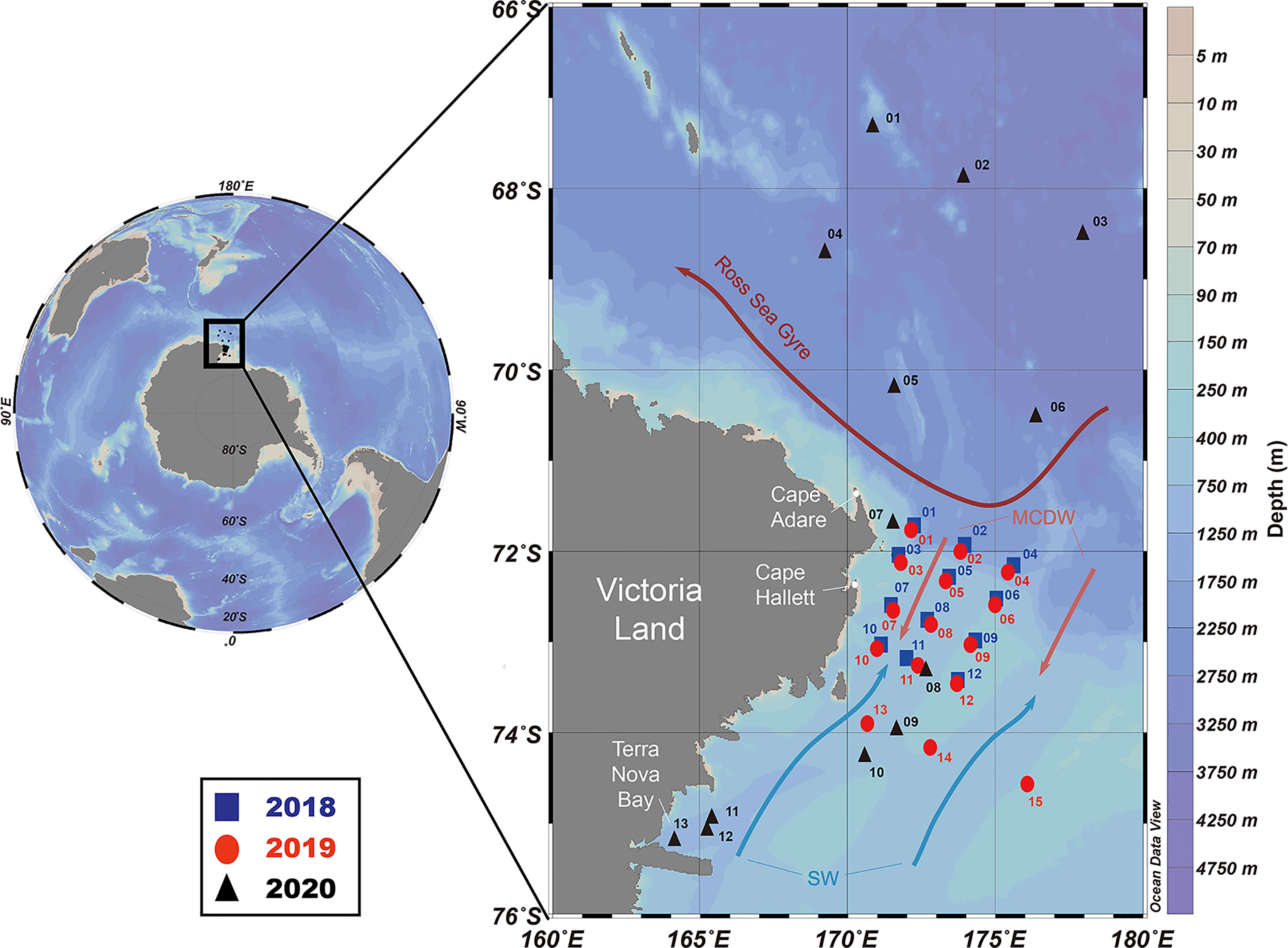
Figure 1 Map of the research area showing sampling stations from 2018 to 2020 in the western Ross Sea region marine protected area (RSR MPA). Arrows represent the Ross Sea Gyre (dark red), SW (light blue), and MCDW (light red). SW, shelf water; MCDW, modified circumpolar deep water.

Data Collection and Sample Processing

Mesozooplankton were vertically collected from an approximate depth of 200 m by using a Bongo net (mesh size: 330 µm, mouth diameter: 0.6 m) equipped with a flow meter. The water volume was estimated by multiplying the mouth area of the net by the maximum depth reached (200 m). The collected samples were quantitatively subsampled using a Folsom plankton splitter. The collected samples were immediately fixed in 5% filtered seawater formalin and then transported to the laboratory. The observation and identification of the samples were carried out under a dissecting microscope (Zeiss STEMI SV8). If necessary, the appendages were dissected and observed under a compound microscope (Olympus BX51).

Seawater temperature (Temp), salinity (Sal), dissolved oxygen (DO), and fluorescence were obtained by using a conductivity-temperature-depth (CTD) system (Sea-Bird, SBE 911plus) with an oxygen sensor at all sampling stations. All data were averaged into 1-m depth intervals to eliminate undesirable noise.

Water samples to measure chlorophyll-a (Chl-a) and nutrients (PO₄, NO₃+NO₂, NH₄, and SiO₂) were collected from the surface to 100 m using a 10-L PVC Niskin water sampler attached to a CTD sampler, but this sampling was not conducted in 2020. The collected samples (0.3 to 0.5 L) for Chl-a concentration were filtered through 25 mm GF/filter paper (Whatman, 0.7 µm pore). Then, the water samples (0.6 to 1.0 L) were filtered continuously through 20 μm and 5 μm membrane filters (47 mm), and 47 mm GF/F filters (Whatman, 0.7 μm pore). Size-fractionated Chl-a was treated as Chl-a_micro (over 20 μm), Chl-a_nano (5−20 μm), and Chl-a_pico (0.7−5 μm) (Liu et al., 2013). All filtered samples were extracted in 90% acetone in the dark for 24 hours (Parsons et al., 1984), and then Chl-a concentrations were measured using Trilogy (Turner Designs, USA). Samples for nutrient concentration on board were immediately stored in a refrigerator at 4°C prior to chemical analyses. All nutrient samples were analyzed within two days. Each nutrient concentration was measured using standard colorimetric methods adapted for use on a 4-channel continuous Auto Analyzer (QuAAtro, Seal Analytical).

For the following analyses, the surface and average values of Temp, Sal, and DO from each sampling station were used. The distinction between surface and average value was indicated by subscripts (e.g., Temp_surface and Temp_average) for each data. Only average values were applied for the Chl-a and nutrients. The average values were calculated from the surface to 100 m for Chl-a and nutrients and from the surface to 200 m for Temp, Sal, and DO. The values of Chl-a_total concentrations in 2020 were converted from the fluorescence values by the equation derived from the relationship between total Chl-a_total and fluorescence values of the 2018 and 2019 surveys.

Data Analysis

Species richness (Margalef D), diversity (Shannon-Wiener H′), and evenness (Pielou’s J′) were calculated to explain the characteristics of the mesozooplankton community (Margalef, 1958; Shannon and Weaver, 1963; Pielou, 1966). The following equations were used to calculate the three indices:

$$H’=-{\displaystyle \sum _{i=1}^s{P}_i\left(In{P}_i\right)}$$

$$J’=\frac{H’}{InS}$$

$$D=\left(S-1\right)/InN$$

where H′ is the observed diversity index; P_i is the proportion of the ith species in the population; S is the total number of species; and N is the total number of individuals.

All multivariate analyses in this study were performed by using the PRIMER v7 package (Clarke et al., 2014; Clarke and Gorley, 2015) and PERMANOVA+ for PRIMER (Anderson et al., 2008). For the biotic analyses, a log transformation (X+1) was carried out before analyses to decrease the influence of highly abundant species in the following analyses (Majewski et al., 2017). A resemblance matrix based on Bray–Curtis dissimilarity was created to identify between-station dissimilarities. Hierarchical cluster analyses (CLUSTER) were conducted based on the Bray–Curtis dissimilarities using group-average linking. As a result, the mesozooplankton community was divided into several groups according to the group similarity. Similarity profile (SIMPROF) permutation tests were simultaneously performed with CLUSTER to determine whether the separated groups exhibited statistically significant (P < 0.05) differences (Clarke et al., 2008). The null hypothesis was rejected if the significance level (P) was <0.05. The groups including only one station were considered outliers and removed from further analyses (Valesini et al., 2014). Nonmetric multidimensional scaling (nMDS) ordination was performed to depict the spatial patterns associated with the sampling stations. PERMANOVA was carried out to verify differences between groups. Similarity percentage (SIMPER) analyses were conducted to determine which species contributed to the observed differences between groups. Principal coordinate analyses (PCoA) were conducted to depict correlations with species and environmental factors that contributed to group differences based on the SIMPER analysis.

For the environmental analyses, draftsman plots were constructed based on environmental data to select an appropriate transformation (Valesini et al., 2014). As a result, log transformations (X+1) were carried out for Sal_average and DO_surface in 2018, Sal_surface, DO_surface, DO_average, PO₄, NO₃+NO₂, and NH₄ in 2019, and Sal_surface in 2020. All the environmental data were normalized to ensure that the variables had the same scale (Valesini et al., 2014). A resemblance matrix of environmental data was created based on the Euclidean distance dissimilarity. A PERMANOVA was performed to test whether environmental factors had statistically significant (P < 0.05) differences according to the zooplankton community groups. The biological-environmental (BIOENV) procedure was used to explore which environmental factors best explained the differences in the mesozooplankton communities. A nonparametric multivariate linkage tree (LINKTREE) was performed to determine which environmental factors divided different assemblage groupings based on the environmental factors derived from the BIOENV analysis.

Results

Environmental Factors

The ranges of the environmental factors among the sampling stations are summarized in Table 1 and Figures 2, 3. When comparing environmental factors by year, these factors represented significant differences across the three surveys (pseudo-F = 9.7102, P < 0.05). Additionally, the Temp_surface was highest (0.12°C) in 2019 and lowest (‒0.19°C) in 2020. The Temp_average in 2018 and 2019 showed a small difference, but a relatively wide temperature range, from ‒1.89 to 0.13°C, was observed in 2020. Although the temperature in 2020 had a wider range than that observed in 2018 and 2019, similar salinity values were observed each year. Both DO_surface and DO_average showed similar patterns each year and tended to show opposite trends to Temp_surface. DO_surface and DO_average values were the highest in 2020 followed by 2018 and 2019, with the lowest value (254.04 mg/L) in 2020 and the highest (371.79 mg/L) in 2020. The DO_surface average value was lower than DO_average in each year, and the former had a far wider range than the latter. When comparing environmental factors in each year, station 10 in 2018 had the lowest Sal_average, DO_surface, and DO_average values compared to the other stations. In 2019, Temp_surface showed low values at stations near land. Station 13 indicated the lowest values in Temp_average and Sal_surface and the highest value in DO_average. Except for Sal_average and DO_surface, environmental factors were associated with latitude in 2020. The water temperatures were low at the southern stations but high at the northern stations. Sal_surface and DO_average were higher at the northern stations than at the southern stations. The Chl-a_total concentration was higher in 2018 than in 2019 and 2020. Because size-fractionated Chl-a and nutrients were not sampled during the 2020 survey, these data were compared for only two surveys, 2018 and 2019. The Chl-a_micro concentration had a much wider range of values at the 2018 stations than the 2019 stations. The size-fractionated Chl-a concentrations that could be distinguishable by latitude in 2018 did not follow the same trend in 2019. The southern stations in 2018 represented much higher Chl-a_micro concentrations than those from the other stations in both 2018 and 2019. Higher concentrations of PO₄ and NH₄ were observed in 2018, whereas the NO₃+NO₂ concentration was higher in 2019. The concentration of SiO₂ exhibited a much wider range of values in 2019 than in 2018. The NH₄ concentration was distinguished by latitude in 2019 but not in 2018.

TABLE 1

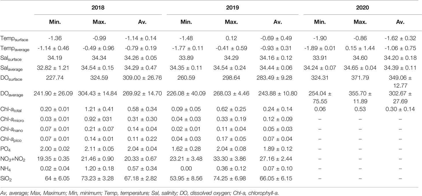
Table 1 Summary of the environmental factors monitored during each survey in the RSR MPA.

FIGURE 2

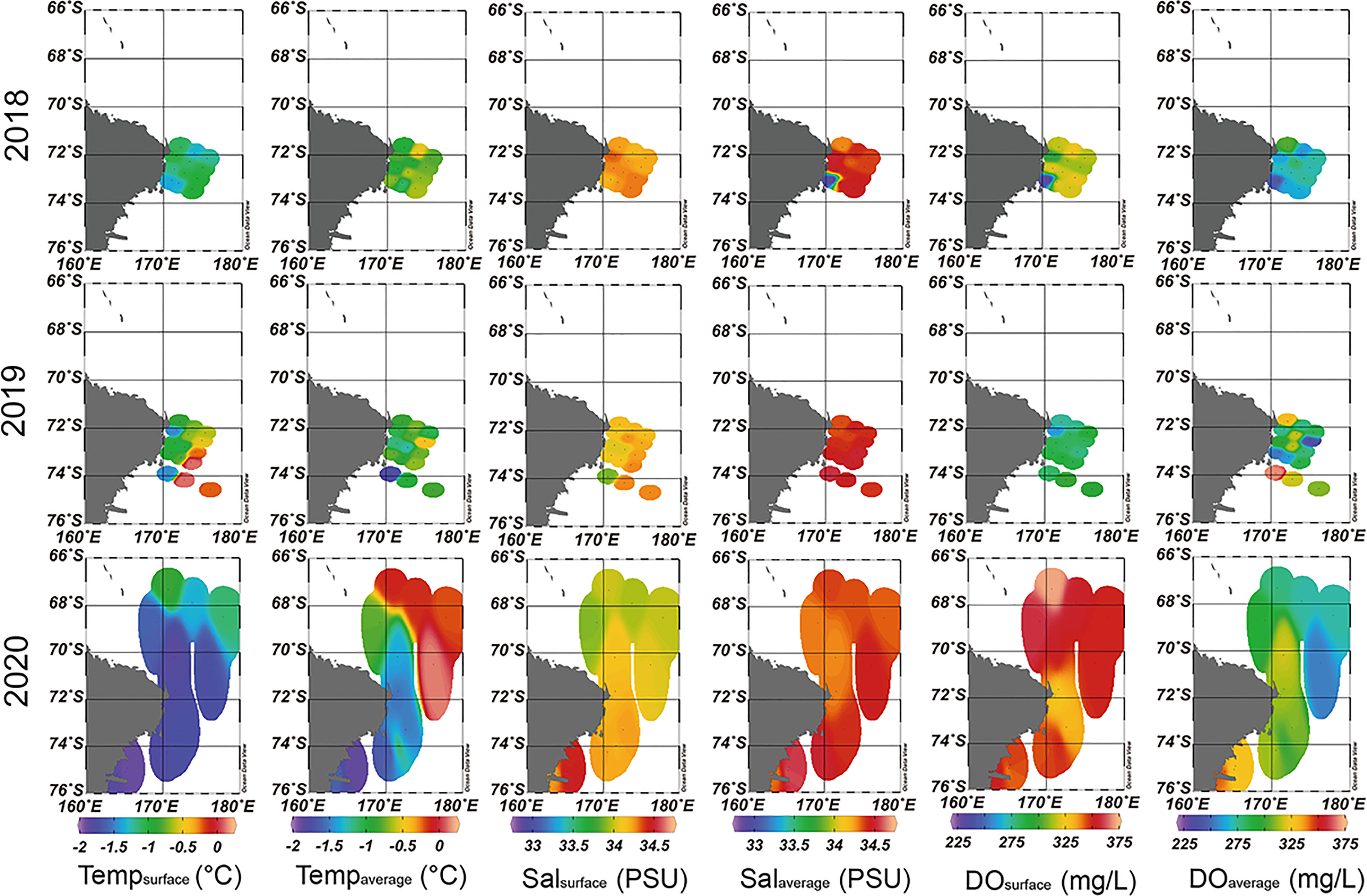
Figure 2 Spatial and temporal pattern of the environmental factors in the western Ross Sea region marine protected area (RSR MPA) from 2018 to 2020.

FIGURE 3

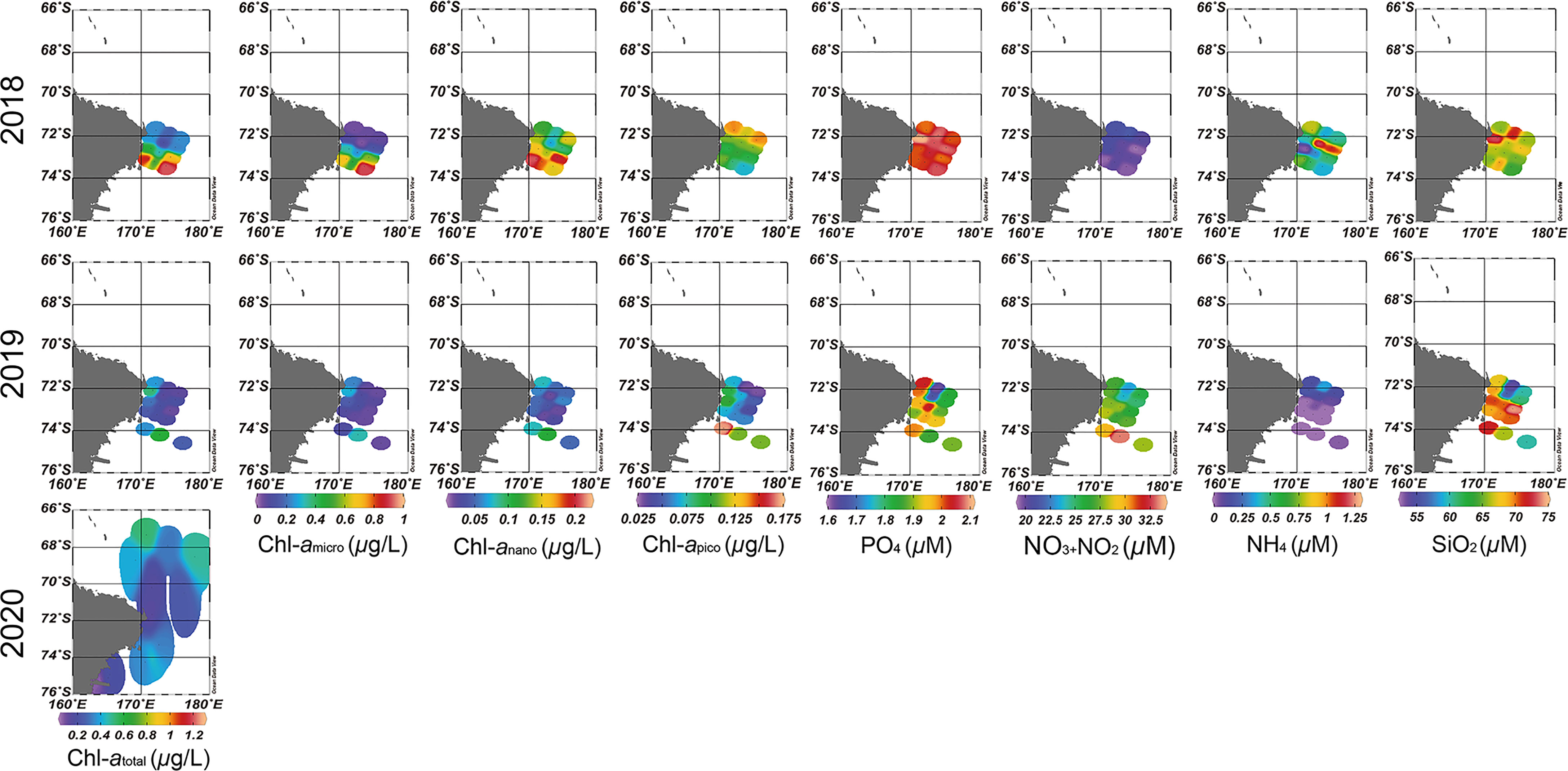
Figure 3 Spatial and temporal pattern of the Chl-a and nutrients in the western Ross Sea region marine protected area (RSR MPA) from 2018 to 2020.

Mesozooplankton Community Structure

In the present study, 33 mesozooplanktonic taxa were identified from 2018 to 2020 (Supplementary Table 2 and Figure 4). From 2018 to 2020, the total mesozooplankton abundances ranged 5.97 to 1,269.89 ind./m³ with a mean total abundance of 119.77 ind./m³. A total of 30 species and 59.4 ind./m³, 30 species and 21.98 ind./m³, and 28 species and 288.26 ind./m³ were observed in 2018, 2019, and 2020, respectively (Supplementary Table 2 and Figure 4). Although an equal number of species were identified in 2018 and 2019, the abundance was three times higher in 2018 than in 2019. Although the smallest number of species was identified in 2020, the highest abundance was observed during the 2020 survey. The highest abundance of individuals was attributed to pteropods, including L. helicina antarctica. Copepods were the dominant species, accounting for 46‒53% of the total number of species for all periods. Pteropods, including L. helicina antarctica, had the greatest total abundance in 2020, accounting for 70% of the total abundance that year, whereas copepods were the most abundant taxon in 2018 and 2019. When comparing ecological indices by year, the mean D was highest in 2019, followed by 2018 and 2020, whereas the mean H´ and J´ were highest in 2018, followed by 2019 and 2020 (Supplementary Table 2 and Figure 4). Additionally, the mean D and H´ of each station indicated significant differences across the three surveys (P < 0.05 for species richness; P < 0.05 for diversity) whereas the mean J´ did not (P > 0.05). Consequently, the community in 2018 was more stable than those in the other surveys, while the community in 2020 was relatively less stable. This result is supported by the abundance of the pteropods in 2020, which was much higher than that in the other surveys.

FIGURE 4

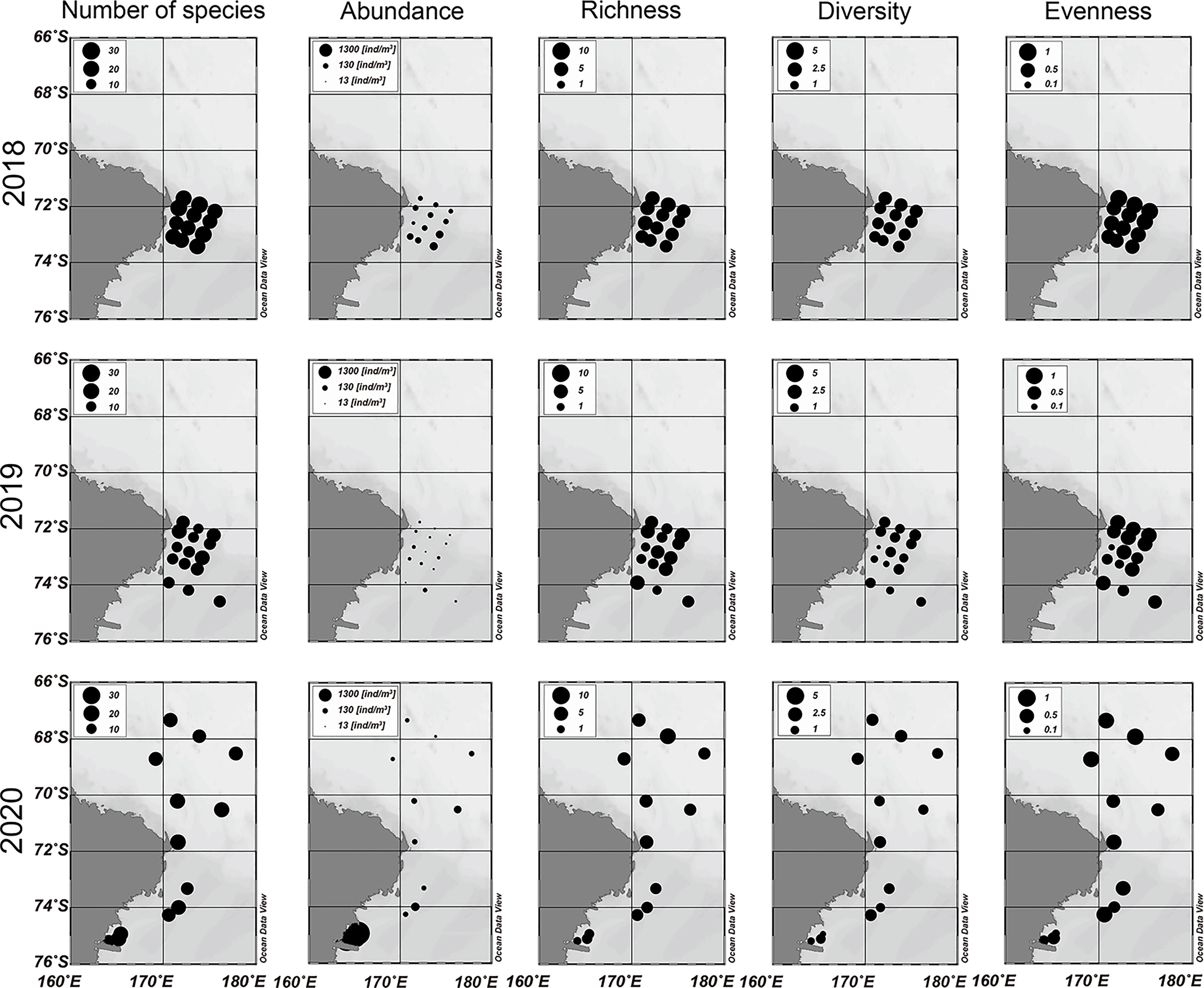
Figure 4 Spatial and temporal distribution pattern of the mesozooplankton community in the western Ross Sea region marine protected area (RSR MPA) from 2018 to 2020.

Spatial Distribution of the Mesozooplankton Community

Hierarchical cluster analysis divided the mesozooplankton community of 2018 into two groups at a dissimilarity level of 45.05%, which was statistically significant (SIMPROF, P < 0.05, n = 999) (Figure 5). Although group B could be divided into two subgroups (B1 and B2) at the 32.87% dissimilarity level, the null hypothesis that there was no difference in species composition within group B was not rejected at a level of the statistical significance level of 5% (SIMPROF, P > 0.05, n = 999) (Figure 5). Additionally, the two groups were well separated from each other in the nMDS plot, supporting the results of the cluster analysis (stress = 0.06) (Figure 5). Station 7, which was the sole member of group A, was located far from the other stations. Station 7 had the lowest total number of species and mesozooplankton abundance in 2018 (Supplementary Table 3). The stations in group B were loosely connected. In the PERMANOVA, the null hypothesis that there was no difference in the mesozooplankton community between groups A and B was not rejected at a significance level of 5% (pseudo-F = 3.4271, P > 0.05) (Table 2). Consequently, the taxa observed in 2018 seem to form a single community. The data for station 7, with the lowest total number of species and abundance, affected the results of the cluster analysis and SIMPROF test.

FIGURE 5

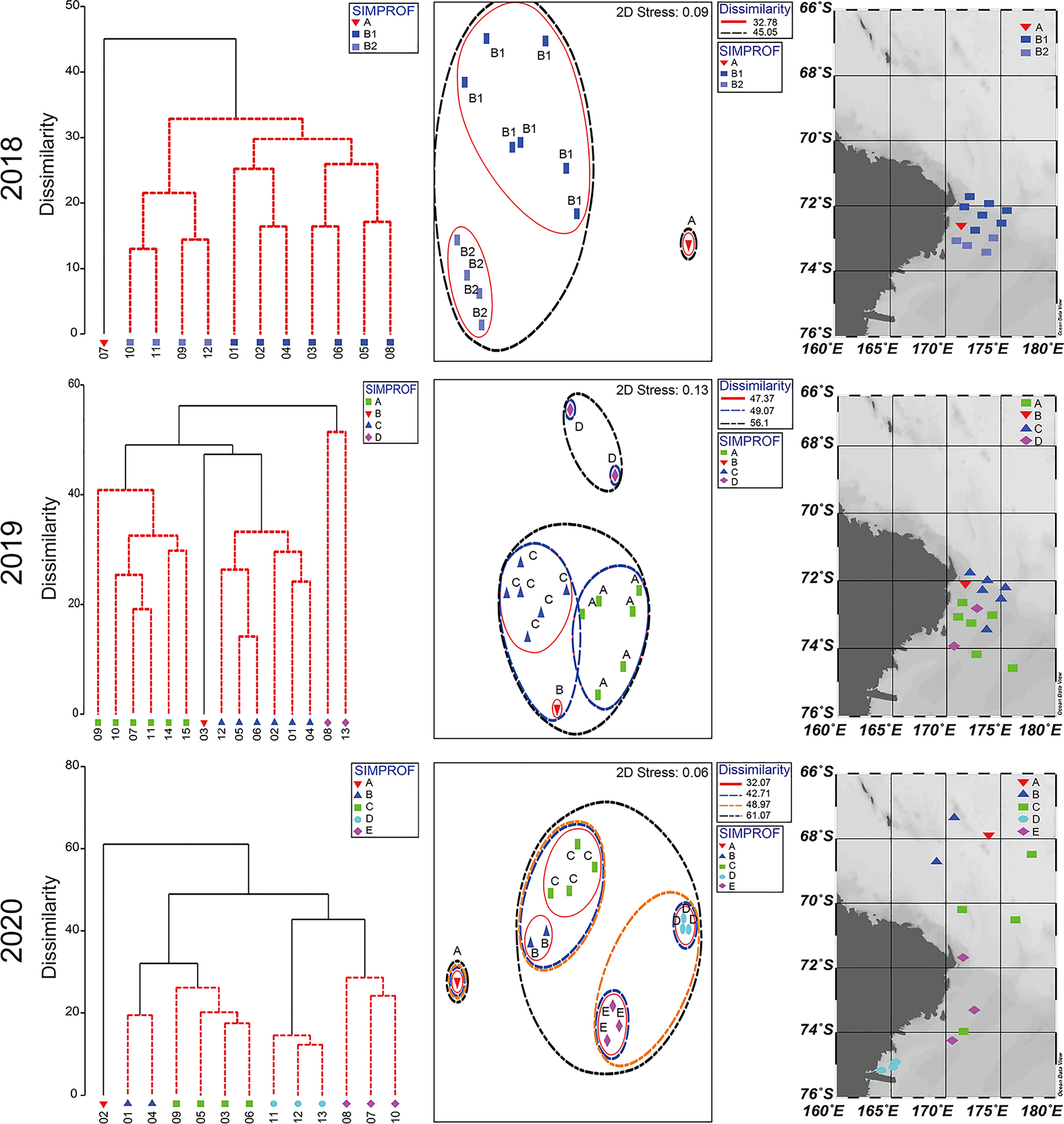
Figure 5 Dendrograms (left) indicating significant differences (P < 0.05) by black lines, nonparametric multidimensional scaling (NMDS) plots (middle) of the sampling stations, and maps (right) showing divided groups according to the SIMPROF.

TABLE 2

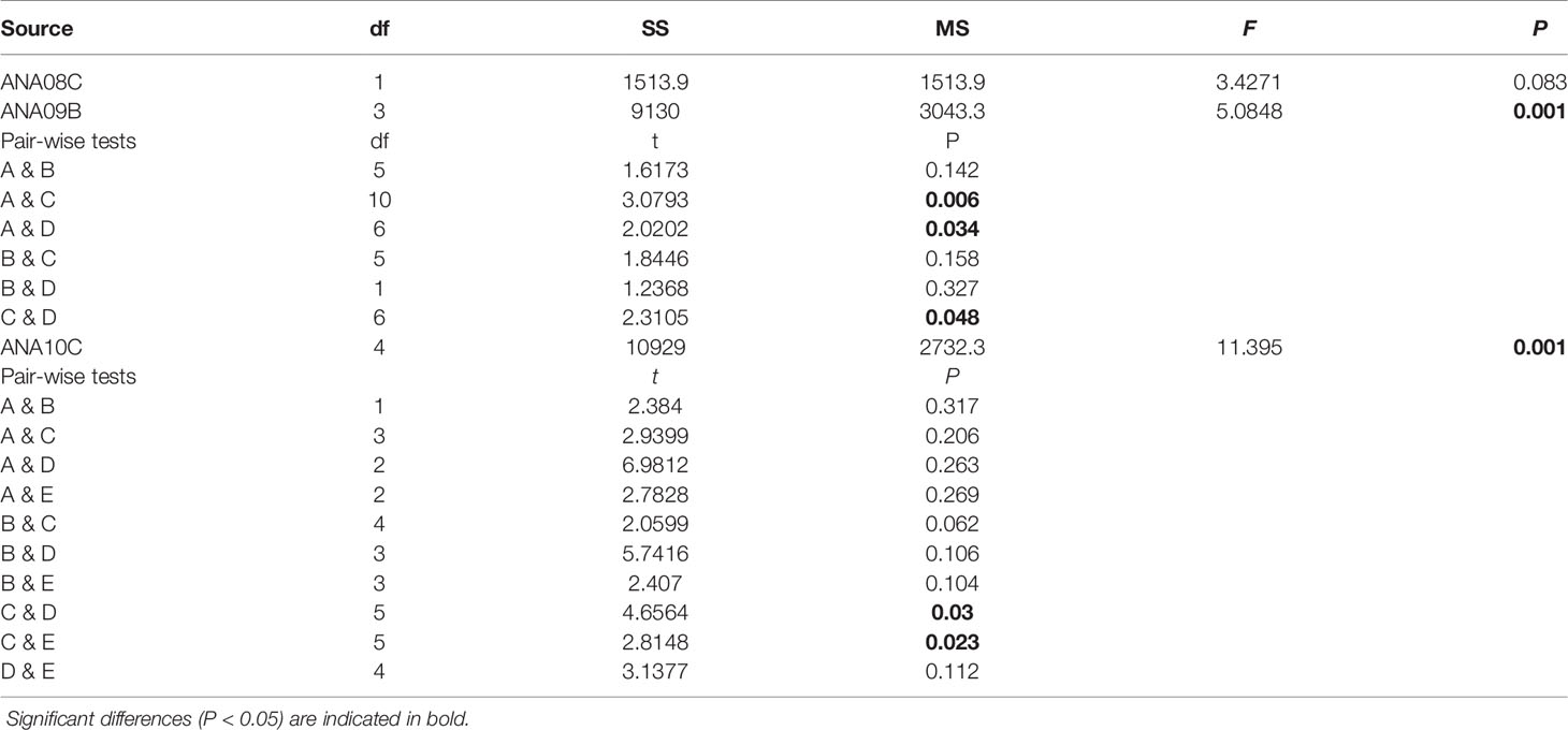
Table 2 Results of PERMANOVA based on log-transformed species abundance data according to groups and between (pairwise tests) groups from each survey.

Hierarchical cluster analysis of 2019 divided the mesozooplankton community into four significantly different groups (SIMPROF, P < 0.05, n = 999) (Figure 5). The dendrogram was first divided into group D and a group combining A, B, and D together at a dissimilarity level of 56.1% (P < 0.05). Group A was separated from groups B and C at a dissimilarity level of 49.07% (P < 005). Groups B and C were separated from each other at a dissimilarity level of 47.37% (P < 0.05). The stations were grouped close together in this survey, supporting the results of the cluster analysis shown in the nMDS plot (stress = 0.13) (Figure 5). The stations associated with group D were located far from the other stations. Very low abundance at these stations was observed (Supplementary Table 4). PERMANOVA demonstrated that there were significant differences between the groups (pseudo-F = 5.0848, P < 0.05). Pairwise comparisons in the PERMANOVA showed a significant difference between each pair of groups except for groups A and B (P > 0.05), B and C (P > 0.05), and B and D (P > 0.05) (Table 2).

Hierarchical cluster analysis separated the mesozooplankton community observed in 2020 into five significantly different groups (SIMPROF, P < 0.05, n = 999) (Figure 5). Group A was first separated from the other groups, including groups B, C, D, and E, at a dissimilarity level of 61.07% (P < 0.05). Groups B and C were separated from groups D and E at a dissimilarity level of 48.97% (P < 0.05). The former set of groups was subdivided into groups B and C at a 32.07% dissimilarity level (P < 0.05), and the latter was subdivided into groups D and E at a 42.71% dissimilarity level (P < 0.05). The stations in this survey were grouped close together, supporting the results of the cluster analysis shown in the nMDS plot (stress = 0.06) (Figure 5). Group A, including only one station (ANA10C-02), was located far from the other groups on the nMDS plot. In 2020, the lowest mesozooplankton abundance was observed at station 2 (Supplementary Table 5). PERMANOVA demonstrated that there were significant differences between the groups (pseudo-F = 11.395, P < 0.05); however, pairwise comparisons in the PERMANOVA showed no significant difference between each pair of groups (P > 0.05) (Table 2). Exceptions were detected between groups C and D (P < 0.05) and between groups C and E (P < 0.05). As a result, group C is expected to have a significantly different community than groups D and E.

Discriminating and Typifying Mesozooplankton Taxa

In the PCoA of data from 2018, the first two principal coordinate axes explained 40.6% and 25.2% of the variance in the Bray–Curtis dissimilarity matrix, respectively (Figure 6). The first axis separated the stations into B1, including stations 1, 2, 3, 4, 5, 6, and 8 (on the right), and B2, including stations 9, 10, 11, and 12 (on the left). In the SIMPER analysis, the average dissimilarity of groups B1 and B2 was 32.87%, and eleven species contributed to the group dissimilarity of the upper 80% (Table 3). Among these species, four (Euphausia spp., Sagitta spp., Unidentified Ostracoda, and Paraeuchaeta antarctica) showed higher average abundances in B1 than B2, while seven other species (Ctenocalanus sp., Oithona spp., L. helicina antarctica, Calanoides acutus, Polychaeta larvae, Oncaea spp., Metridia gerlachei) presented higher average abundances in B2 than B1 (Figure 6; Table 3).

FIGURE 6

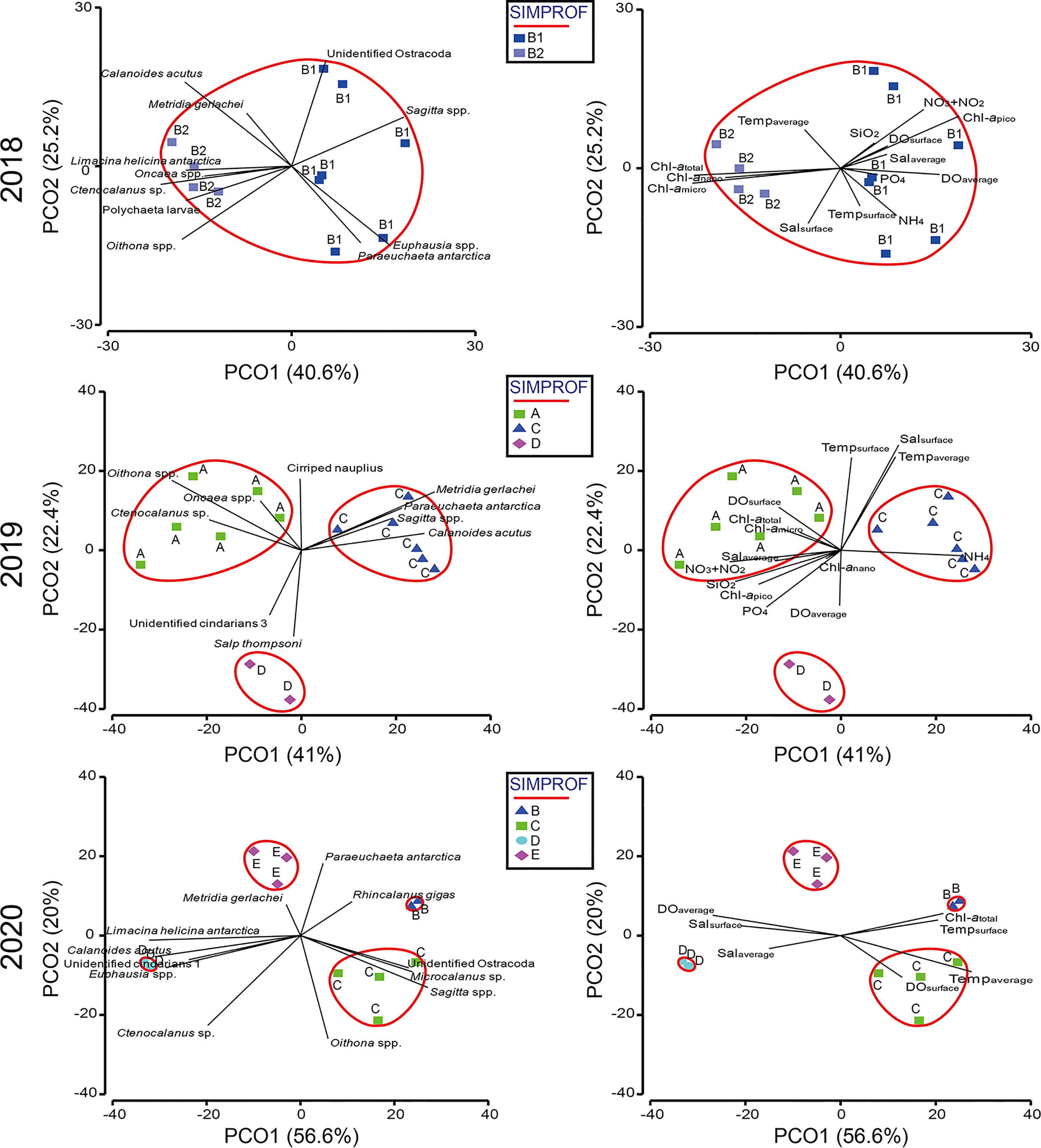
Figure 6 Principal coordinate analysis (PCoA) plots based on log-transformed species abundance data and environmental factors. Dominant species (left) and environmental factors (right).

TABLE 3

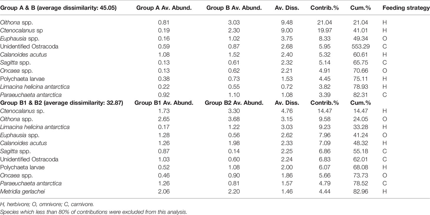
Table 3 Results of the SIMPER analysis, showing species that contribute to the dissimilarity between the groups of the 2018 survey.

In the PCoA of data from 2019, the first two principal coordinate axes explained 41% and 22.4% of the variance in the Bray–Curtis dissimilarity matrix, respectively (Figure 6). The first axis separated group C (on the right) from groups A and D (on the left), whereas the second axis divided group D (on the bottom) from groups A and C (on the top). According to the SIMPER analysis, the average dissimilarity of groups A and C was 49.36%, and eight species contributed to the group dissimilarity of the upper 80% (Table 4). Among these species, four (Oithona spp., Ctenocalanus sp. Cirriped nauplius, and Oncaea spp.) had higher average abundances in group A than in group C, whereas the average abundances of other species followed the opposite trend. Groups A and D had an average dissimilarity of 54.95% and included seven species with dissimilarities of the upper 80%. Only two species, Salp thompsoni and Unidentified cnidarians 3, had higher average abundances in group D than in group A. The average dissimilarity of groups C and D was 56.70%, and nine species contributed to the group dissimilarity of the upper 80%. Among those nine species, three (S. thompsoni, Unidentified cnidarians 3, and Ctenocalanus sp.) had higher average abundances in group D than in group C. The correlations between the abovementioned ten species and groups indicated that three species, Ctenocalanus sp., Oncaea spp., and Oithona spp., were strongly associated with group A. Four species, M. gerlachei, C. acutus, P. antarctica, and Sagitta spp., were correlated with group C. Two species, S. thompsoni and unidentified cnidarians 3, showed a strong correlation to group D (Figure 6).

TABLE 4

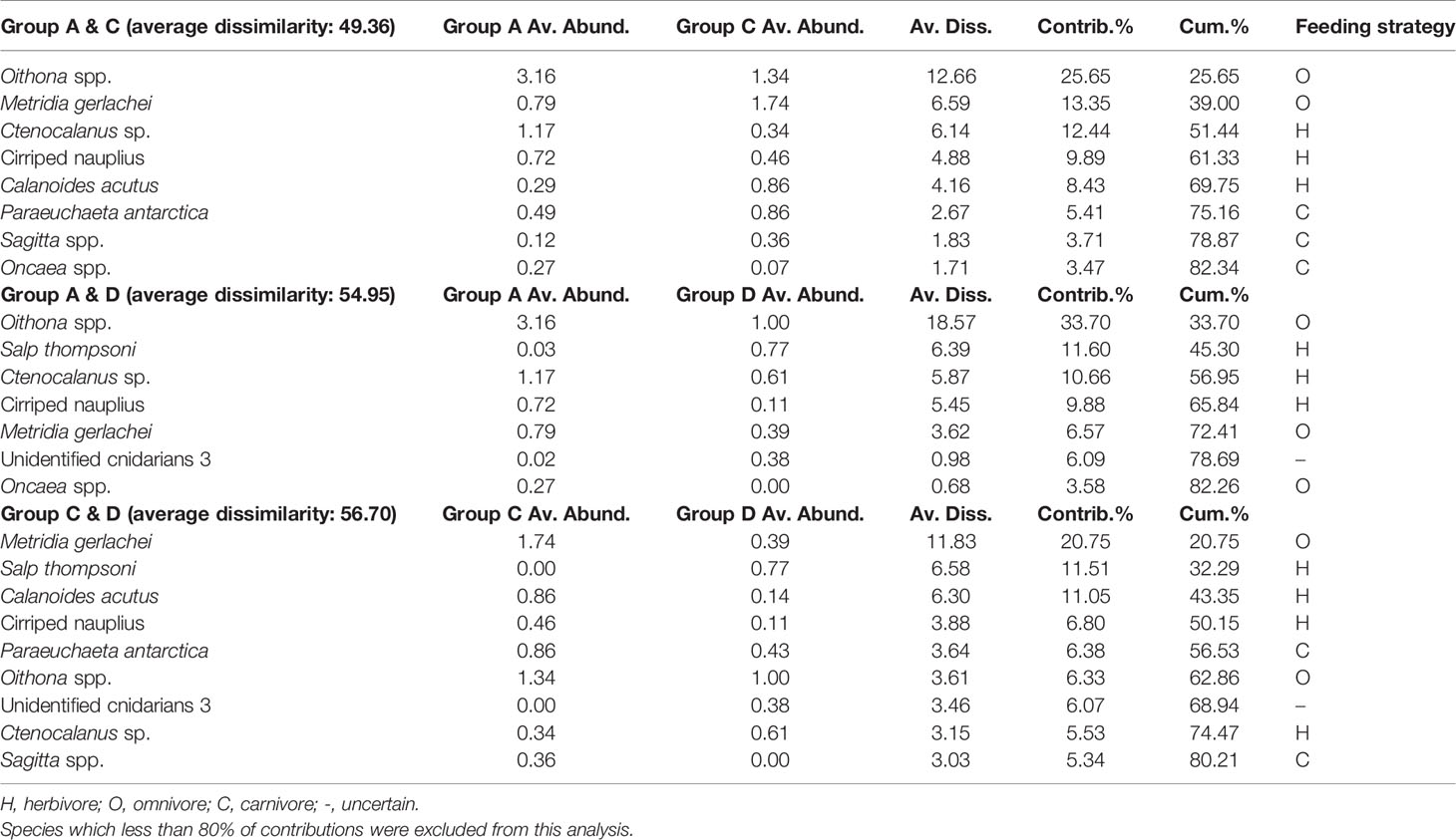
Table 4 Results of the SIMPER analysis, showing species that contribute to the dissimilarity between the groups of the 2019 survey.

In the PCoA plot of 2020, the first two principal coordinate axes explained 56.6% and 20% of the variance in the Bray–Curtis dissimilarity matrix, respectively (Figure 6). The first axis separated groups B and C (on the right) from groups A and D (on the left), whereas the second axis divided groups B and E (on the top) and groups C and D (on the bottom), respectively. In the SIMPER analysis, the average dissimilarity of groups B and C was 32.08%, and eight species contributed to the group dissimilarity of the upper 80% (Table 5). Groups B and D had an average dissimilarity of 60.48%, with six species contributing dissimilarities of the upper 80%. The average dissimilarity of groups B and E was 42.57%, with nine species having dissimilarity less than 80%. Groups C and D had an average dissimilarity of 52.45%, with seven species contributing to this value. Seven species contributed to the average dissimilarity between Groups C and E (42.98%). The average dissimilarity between groups D and E was 42.75%, with six species contributing to the dissimilarity. The correlations between the abovementioned species and groups indicated that Rhincalanus gigas had a positive relationship with group B. Group C was strongly related to Microcalanus sp., Oithona spp., Unidentified Ostracoda, and Sagitta spp. Group D showed a positive relationship with C. acutus, L. helicina antarctica, Euphausia spp., and unidentified cnidarians 3. Oithona spp. had a negative relationship with to group E. Ctenocalanus sp. showed a negative relationship with group B (Figure 6).

TABLE 5

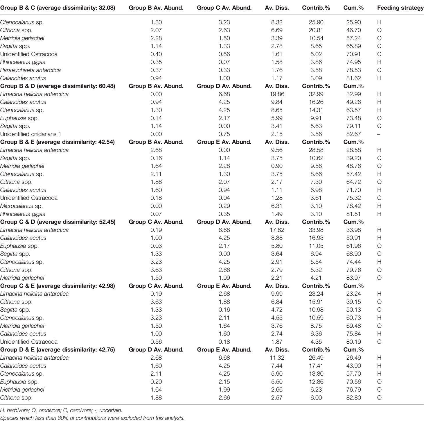
Table 5 Results of the SIMPER analysis, showing species that contribute to the dissimilarity between the groups of the 2020 survey.

Spatial Relationship Between Mesozooplankton Groups and Environmental Factors

In 2018, although the SIMPROF test indicated a significant difference between groups A and B, the comparison between these groups and environmental factors was not performed because group A, which included data from only one station, was excluded from this analysis. However, subgroups B1 and B2 were compared with environmental factors, and the environmental factors associated with these groups differed significantly according to PERMANOVA (PERMANOVA, pseudo-F = 3.3184, P < 0.05) (Table 6). In the PCoA analysis, DO_average, NO₃+NO₂, and Chl-a_pico showed a strong correlation with subgroup B1, whereas Chl-a_total, Chl-a_micro, and Chl-a_nano were strongly related to subgroup B2 (Figure 6). In the BIOENV analysis, the results indicated that 2018 was best described by a combination of Temp_average, Chl-a_total, Chl-a_micro, Chl-a_nano, and Chl-a_pico (BIOENV, ρ = 0.634, P < 0.05) (Table 7). In the LINKTREE analysis, the first division A was separated by the Chl-a_total, Chl-a_micro, or Chl-a_nano concentration (R = 0.73, B% = 91) (Figure 7).

TABLE 6

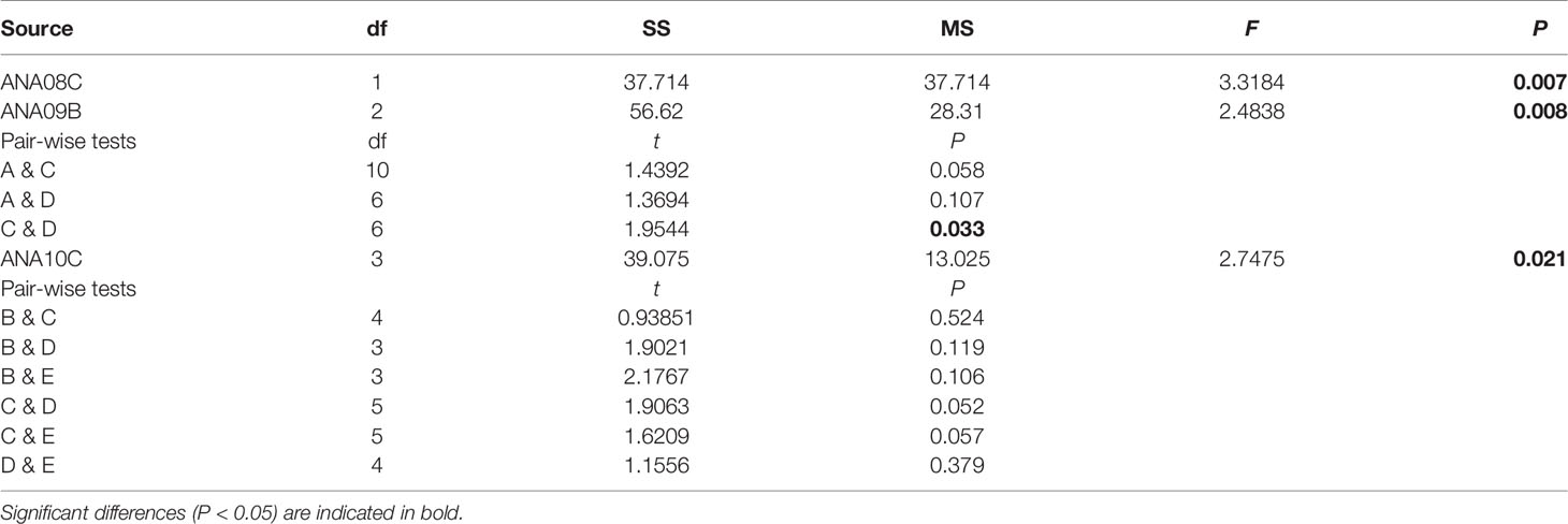
Table 6 Results of the PERMANOVA based on environmental factors according to groups and between (pairwise tests) groups from each survey.

TABLE 7

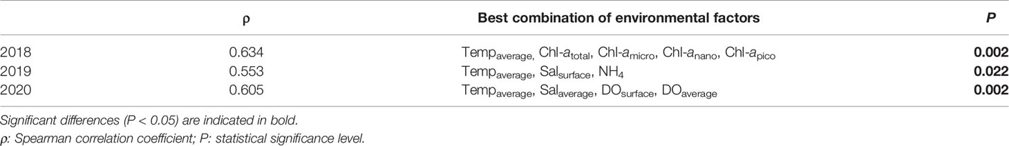
Table 7 Summary of the results of the biological-environment (BIOENV) analysis, showing the best matched combination of environmental factors and mesozooplankton abundances from each survey.

FIGURE 7

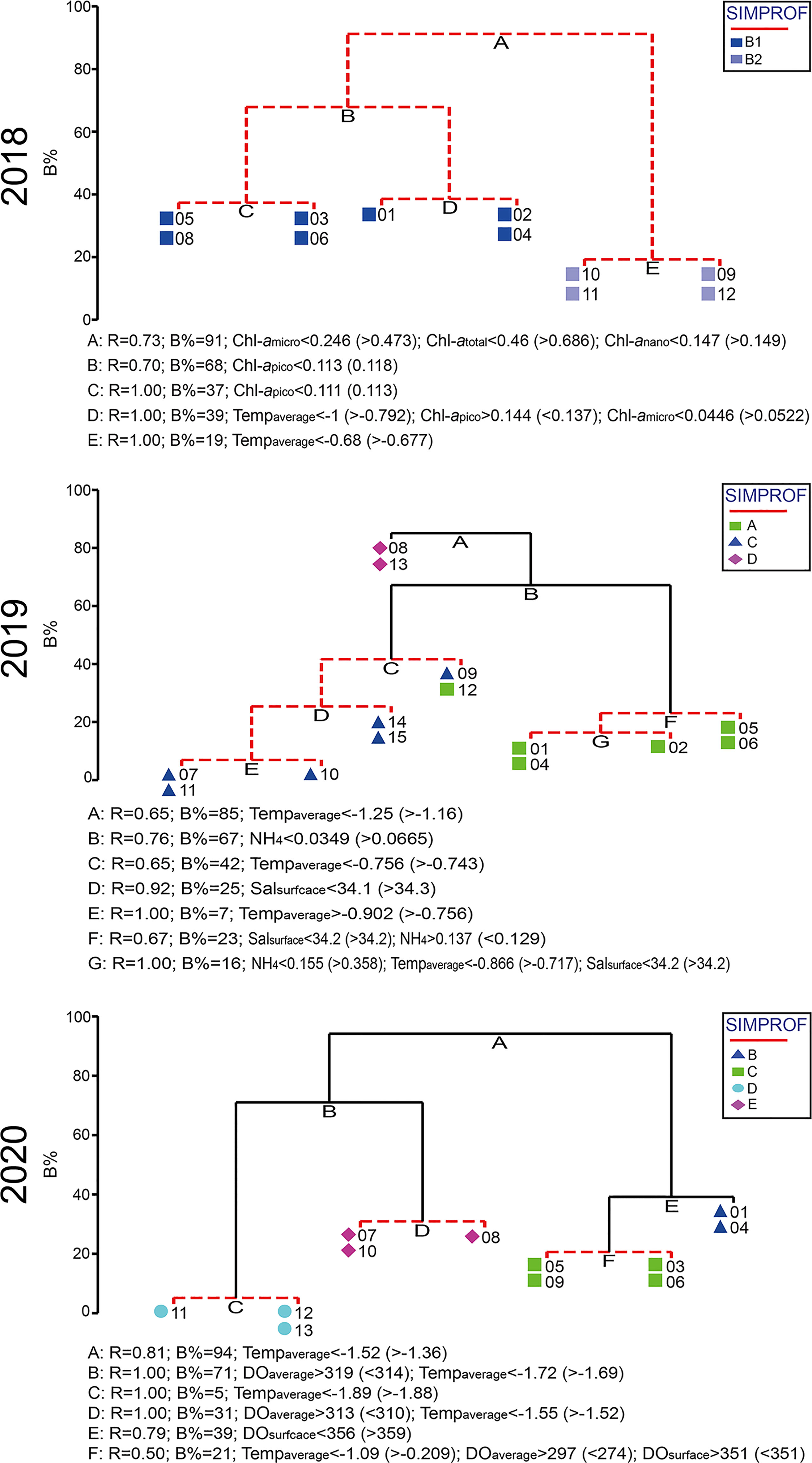
Figure 7 Linkage tree constructed using environmental attributes across all scales as the explanatory data. Stations connected by red lines indicate no significant differences by similarity profile (SIMPROF) analysis.

In 2019, there were significant differences among the environmental factors by group (PERMANOVA, pseudo-F = 2.4838, P < 0.05), and the pairwise comparisons showed no significant difference between groups (P > 0.05) except for groups C and D (P > 0.05) (Table 6). In the PCoA plot, DO_surface, and NO₃+NO₂ were related to group A. Group C was strongly related to NH₄. Group D showed a negative correlation with Temp_surface, Temp_average, and Sal_surface (Figure 6). In the BIOENV analysis, Temp_average, Sal_surface, and NH₄ (ρ = 0.553, P < 0.05) provided the best match with the community (Table 7). Three significantly different (P <0.05) groups were determined by the LINKTREE analysis, with the SIMPROF results corresponding well with the results of the CLUSTER analysis, although station 12 switched from group C to group D (Figure 7). The first division A was split by Temp_average (R = 0.65, B% = 85). The second division B was separated by NH₄ concentration (R = 0.76, B% = 67).

In 2020, significant differences among the groups were found by PERMANOVA (pseudo-F = 2.7475, P < 0.05); however, pairwise comparisons showed no significant differences between groups (P >0.05) (Table 6). The PCoA indicated that Temp_surface and Chl-a_total were strongly related to group B, Temp_average was associated with group C, and group D was associated with Sal_surface, Sal_average, and DO_average. In the BIOENV analysis, the community was best matched by a combination of Temp_average, Sal_average, DO_surface, and DO_average (ρ = 0.605, P < 0.05) (Table 7). The LINKTREE analysis identified four significantly different (P < 0.05) groups, and the results of this analysis were consistent with those of the CLUSTER analysis (Figure 7). The first division A was split by Temp_average (R = 0.81, B% = 94), while the second division B was separated by DO_average and Temp_average (R = 1.00, B% = 71). Division E, which was significantly different from group D, was split by DO_surface (R = 0.79, B% = 39).

Discussion

Among the 2018, 2019, and 2020 surveys, the surface water temperature was highest in the 2019 survey whereas lowest in the 2020 survey. The timings of the surveys, specifically, February 2018, January 2019, and March 2020, are likely to be relevant for this finding (Smith et al., 2003; Smith et al., 2014; Cau et al., 2021). Given that MCDW is characterized by a subsurface high temperature and low dissolved oxygen, the 2019 survey’s high surface water temperature and low DO were likely influenced by the MCDW (Budillon et al., 2003). Unlike surface water temperature, average water temperature showed greater variability in 2020 than in other surveys. This is thought to be due to the sampling stations in 2020 having a wider geographic range with respect to latitude than that in other years. Regarding the Chl-a concentration, the concentrations in 2018 were about two times higher than those in other surveys. In particular, the southern stations (subgroup B2) in 2018 indicated much higher concentrations than other sampling stations. This high concentration is well corresponding with the finding of Jo et al. (2021) that much higher diatoms concentration in the southern stations. Furthermore, the nutrients such as NO₃+NO₂, PO₄, and SiO₂ were negatively correlated with B2 in the PCoA plot. This negative correlation was related to the phytoplankton biomass because these nutrients can be removed from the environment by autotrophic assemblages (Nelson and Smith, 1986; Smith et al., 2003). Taken all together, given summer bloom can occur in February by diatoms and the timing of the bloom is very consistent, the high Chl-a concentration in 2018 could be related to the summer bloom by diatoms (Edwards and Richardson, 2004; Peloquin and Smith, 2007; Smith et al., 2011; Kaufman et al., 2014; Smith et al., 2014).

Considering the earlier studies covered different regions and employed different methodologies, it is difficult to compare our data that from prior studies in the Ross Sea (Stevens et al., 2015; Smith et al., 2017). However, when a small mesh plankton net (200 µm) was used instead of a coarse plankton net (over 330 µm), the amount of the mesozooplankton was higher (Pane et al., 2004; Elliott et al., 2009; Stevens et al., 2015; Smith et al., 2017). Similar to findings in prior studies, the abundance recorded in this study using a coarse mesh-sized plankton net was lower than that reported in the survey using a fine mesh-sized plankton net (Pane et al., 2004; Stevens et al., 2015; Smith et al., 2017). The mesozooplanklton community, however, was dominated by small species (e.g. Oithona spp., Ctenocalanus sp., etc.). The composition of the mesozooplankton community was similar to that in previous studies (Pane et al., 2004; Stevens et al., 2015; Grillo et al., 2020). Therefore, the mesozooplankton sampling region and methodology are regarded as significant factors influencing the survey’s conclusion (Stevens et al., 2015; Smith et al., 2017).

Given the mesozooplankton community of the present study, our analyses of data from 2018, 2019, and 2020 surveys showed that the mesozooplankton community in the western RSR MPA could be separated by spatio-temporal variability. Taxa observed in 2019 and 2020 could be divided into four and five significantly different groups, respectively. Although there were no significantly different groups among the taxa observed in 2018, the community structure could be distinguished by the feeding strategy of the dominant species. Additionally, the subgroups of 2018 and groups of 2019 and 2020 showed significant differences according to environmental factors.

In 2018, Euphausia spp., P. antarctica, Sagitta spp., and unidentified Ostracoda were strongly correlated with subgroup B1, whereas C. acutus, Ctenocalanus sp., M. gerlachei, Oithona spp., Oncaea spp., and Polychaeta larvae were strongly correlated with subgroup B2. The dominant species in B1 had omnivorous or carnivorous feeding modes, whereas the dominant species in B2 were mostly herbivorous (Hopkins, 1987; Lopez and Huntley, 1995; Pasternak and Schnack-Schiel, 2001; Bocher et al., 2002; Ward and Hirst, 2007; Elliott et al., 2009; Grillo et al., 2020). According to the LINKTREE analysis, the stations included in subgroup B2 had much higher Chl-a_total, Chl-a_micro, and Chl-a_nano concentrations than those included in subgroup B1. In accordance with the previous studies and the present study, the relatively high Chl-a_micro concentration of subgroup B2 recorded in 2018 was likely to result of summer blooms by diatoms (Peloquin and Smith, 2007; Smith et al., 2011; Kaufman et al., 2014; Smith et al., 2014; Jo et al., 2021; Saggiomo et al., 2021). As a result, herbivorous zooplankton increased in B2, while B1 was characterized by relatively high abundances of omnivorous or carnivorous species. Thus, the Chl-a concentration gradients throughout the region could be considered the main factor regulating the mesozooplankton community in 2018. This finding is consistent with the previous reports, which found that foods such as Chl-a are the main factors regulating mesozooplankton distribution (Liu and Dagg, 2003; Chen et al., 2017; Smith et al., 2017).

In the 2019 survey, Ctenocalanus sp. and Oithona spp., and Oncaea spp. were correlated with group A; C. acutus, M. gerlachei, P. antarctica, Sagitta spp., and Unidentified Ostracoda were positively associated with group C; and S. thompsoni and Unidentified cnidarians 3 were positively correlated with group D. Even though group D had a much lower abundance than the other groups, the SIMPER analysis indicated that the abundances of S. thompsoni and Unidentified cnidarians 3 were higher than the abundances observed in the other groups. Small species such as Ctenocalanus sp. and Oithona spp. were dominant in group A, whereas relatively large species such as C. acutus and M. gerlachei were more common in group C. In other words, small species were common in group A, while relatively larger species were more common in group C. Regarding environmental factors, group D was separated from the other groups at a much lower temperature. Group A was separated from group C by a lower NH₄ concentration. The food resources (e.g., Chl-a) did not have a significant relationship with the groups in 2019, unlike 2018. Taken all together, these results indicate that the dietary components, such as Chl-a, did not affect the mesozooplankton community structure in 2019. Considering that MCDW intrudes over the Ross Sea at the beginning of January and that water temperature in which group D was found was significantly lower than that of the water in which the other groups were found, it is possible that group D was disturbed by aperiodic intrusion (Smith et al., 2007; Castagno et al., 2017). As a result, the very low abundance at the corresponding stations was confirmed to distinguish them from other groups. Additionally, Biggs (1982) report that ammonium excretion is highly correlated with zooplankton body size corresponds well with the discrimination between groups A and C according to the body size of the dominant species. Large herbivorous species, C. acutus, and large carnivorous taxa such as P. antarctica and Sagitta spp. represented a relatively higher abundance in group C than in group A, whereas small omnivorous species such as Oithona spp. were more abundant in group A than in group C. In summary, regardless of the feeding strategy, the large species were more abundant in group C, whereas relatively small species were common in group A. This differentiation based on size would be related to the predation of small species by large species because trophic processes in the plankton community are highly dependent on the food size (Nelson and Smith, 1986; Lancelot et al., 1993; Hansen et al., 1997; Bocher et al., 2002; Tang et al., 2008; Chen et al., 2017; Sun et al., 2021).

In 2020, there have been more divided groups than in other surveys. This result was thought to be that the 2020 survey included open sea and Terra Nova Bay stations which were not contained in the 2018 and 2019 surveys. Groups B and C, which were mostly located in the open western Ross Sea, had similar species compositions. The two groups shared the most abundant species, but the ranking of those species differed. Groups D and E, which were mainly located on the continental shelf of the western Ross Sea, had similar species compositions; however, group D had a much higher abundance than group E. According to LINKTREE analysis, groups D and E could be separated from groups B and C by having a lower Temp_average. This distinction is likely a result of the geographic distributions of these groups since groups B and C can be separated from groups D and E according to their latitudinal location. Consequently, the Temp_average mainly determined these significant differences between the open sea and continental shelf regions of the western Ross Sea in 2020.

When comparing of the mesozooplankton community structures according to the interannual variations (Figure 8), this comparison can be summarized in a few points: (1) the sampling stations were well clustered according to the survey periods; (2) the stations of 2018 clustered into a single group; (3) the stations in 2019 were separated into two groups, and one of the groups was more similar to the group including the 2018 stations than to another group of 2019; (4) the Terra Nova Bay stations were clustered far from other stations; (5) the stations located in the open Ross Sea in 2020 were much more similar to the stations included in 2018 than to the stations in 2020 on the continental shelf. PERMANOVA indicated that there were significant differences between the groups (pseudo-F = 10.367, P < 0.05). These significant differences were the same in the comparison between the stations excluding open sea stations (pseudo-F = 9.4362, P < 0.05). By the dominant taxa, Oithona spp., which are known to be affected by water temperature, showed a wide distribution range according to the surveys in this study (Ward and Hirst, 2007). Specifically, this species showed a strong correlation with high-latitude stations in 2018 and 2019. However, Oithona spp. was strongly correlated with the open sea, including the low-latitude stations in 2020. Limacina helicina antarctica, which has a high abundance in the southern Ross Sea, had a significantly high abundance at the continental shelf stations in 2020, especially near Terra Nova Bay (Hopkins, 1987; Pasternak and Schnack-Schiel, 2007; Elliott et al., 2009). Furthermore, L. helicina antarctica showed relatively low abundance at the stations included in 2019, which indicated comparatively warm temperatures, whereas its abundance in 2018 was intermediate among the three surveys. The greatest abundance of Ctenocalanus sp., which prefers cold water, was found from February to April namely in 2018 and 2020 surveys, while this species showed relatively low abundance in 2019 (Pasternak and Schnack-Schiel, 2007).

FIGURE 8

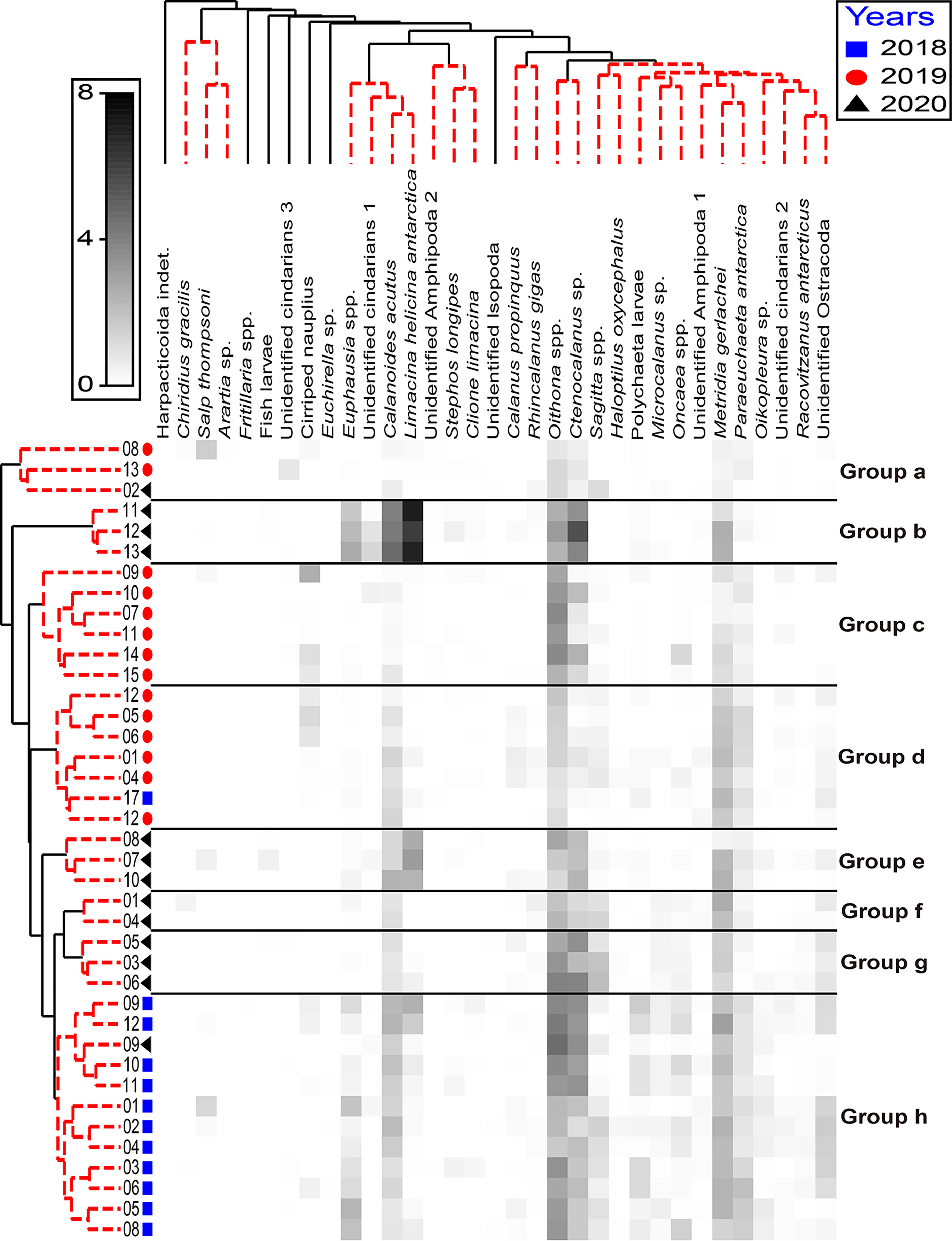
Figure 8 Shade plot based on the log-transformed species abundance data from all the sampling stations; shading intensity is proportional to species abundance. The groups belonging to each station were ordered by similarity profile (SIMPROF) factors, and species were ordered by hierarchical cluster analysis.

Taken together, these results indicate that the mesozooplankton community of the western RSR MPA was altered according to the survey period and differed spatiotemporally. Considering the food resource such as the Chl-a was among the best explanatory factors only in 2018, but not in 2019 and 2020, and the mean total abundance in the 2018 survey is higher than other surveys except for the Terra Nova Bay region, the relatively high Chl-a concentration in late summer induced high mesozooplankton abundance in the western Ross Sea. In other words, if prey, such as phytoplankton or diatoms, were abundant (2018), then the community was influenced by the prey distribution. However, when the abundance of phytoplankton had less influence (2019), the zooplankton community structure was affected by aperiodic intrusions or predation pressure that induced trophic cascades. Predation pressure causing trophic cascades rather than abiotic factors was assumed to be the key factor determining the mesozooplankton community structure in 2019. As the water temperature decreased with latitude and sea ice covered the whole continental shelf (2020), the mesozooplankton community of the western RSR MPA was replaced with species suitable for lower water temperatures. Although the correlation was not significant at the 0.05 level, the Chl-a concentration and mesozooplankton abundance indicated a negative correlation in 2020 (r = -0.547, P > 0.05). Considering the spatial mismatch between phytoplankton and mesozooplankton means both populations asynchrony, this negative correlation is regarded as a typical spatial mismatch between phytoplankton and zooplankton (Edwards and Richardson, 2004; Durant et al., 2013; Mcginty et al., 2014; Sun et al., 2021). This spatial mismatch would be related with the increase of the species that prefer cold water such as L. helicina antarctica which shows a significantly high abundance at the continental shelf stations in 2020.

Conclusion

The results of this study suggest that the mesozooplankton community of the western RSR MPA was influenced by prey if food resources were abundant but affected by predation pressure or environmental factors when food resources were less influential. Therefore, the occurrence of the summer bloom in late summer, mainly in February, is likely to affect the mesozooplankton community in the western RSR MPA. The continental shelf community present in January and February was replaced by species that preferred cold water by March, as the water temperature decreased in the western RSR MPA. These results suggest that climate change will affect the mesozooplankton community of the western RSR MPA in the late summer, because climate change could result in warmer water temperatures and the expansion of sea ice-free periods in the RSR MPA, although the concentration of sea ice has recently increased (Smith et al., 2007; Smith et al., 2014). As a result, the distributions of the species that are mainly found in the western RSR MPA could expand southward. The distribution of the species that prefer cold water, such as L. helicina antarctica and Ctenocalanus sp., could be limited in the southern region. Eventually, the mesozooplankton community currently found in the western RSR MPA would move southward, and a novel zooplankton community could invade the RSR MPA. Considering that the Ross Sea, which is the largest MPA, is an essential feeding area of higher predators such as penguins and whales, these changes in the mesozooplankton community could impact the predation abilities of higher predators, for which zooplankton are the main food resources (Nelson and Smith, 1986; Smith et al., 2012; Smith et al., 2014; Picco et al., 2017; Smith et al., 2017). However, the three surveys in this study were conducted in different months in 2018, 2019, and 2020. Interannual variations can be substantial within the Southern Ocean, and it is possible that these interannual differences were overlooked in this study (Smith et al., 2003; Smith et al., 2014; Cau et al., 2021). Furthermore, the Ross Sea ecosystem has been dramatically influenced by climate change (Smith et al., 2014). Thus, further studies and constant monitoring of the mesozooplankton community in the RSR MPA are required.

Data Availability Statement

The original contributions presented in the study are included in the article/Supplementary Material. The zooplankton and environmental data are available at the Korea Polar Data Center (https://dx.doi.org/doi:10.22663/KOPRI-KPDC-00001925.1). Further inquiries can be directed to the corresponding author.

Author Contributions

HL conceived of the study. BK, BL, NJ, WS, and HL collected and analyzed the environmental data. SK analyzed zooplankton community composition and wrote the manuscript. SK, BK, SL, S-YH, J-HK, and HL contributed to the study design and data discussion. All authors contributed to the article and approved the submitted version.

Funding

This study was a part of a project titled “Ecosystem Structure and Function of Marine Protected Area (MPA) in Antarctica” project (PM21060) funded by Ministry of Oceans and Fisheries, Korea (20170336).

Conflict of Interest

The authors declare that the research was conducted in the absence of any commercial or financial relationships that could be construed as a potential conflict of interest.

Publisher’s Note

All claims expressed in this article are solely those of the authors and do not necessarily represent those of their affiliated organizations, or those of the publisher, the editors and the reviewers. Any product that may be evaluated in this article, or claim that may be made by its manufacturer, is not guaranteed or endorsed by the publisher.

Acknowledgments

The authors thank all those involved in sample collection for their contributions. The authors appreciate the careful assistance of the captain and crew of IBRV Araon.

Supplementary Material

The Supplementary Material for this article can be found online at: https://www.frontiersin.org/articles/10.3389/fmars.2022.860025/full#supplementary-material

References

Anderson M. J., Gorley R. N., Clarke K. R. (2008). PERMANOVA+ for PRIMER: Guide to Software and Statistical Methods (United Kingdom: PRIMER-E: Plymouth).

Google Scholar

Biggs D. (1982). Zooplankton Excretion and NH 4+ Cycling in Near-Surface Waters of the Southern Ocean. I. Ross Sea, Austral Summer 1977–1978. Polar Biol. 1 (1), 55–67. doi: 10.1007/bf00568755

CrossRef Full Text | Google Scholar

Bocher P., Cherel Y., Alonzo F., Razouls S., Labat J., Mayzaud P., et al. (2002). Importance of the Large Copepod Paraeuchaeta Antarctica (Giesbrech) in Coastal Waters and the Diet of Seabirds at Kerguelen, Southern Ocean. J. Plankton Res. 24 (12), 1317–1333. doi: 10.1093/plankt/24.12.1317

CrossRef Full Text | Google Scholar

Budillon G., Pacciaroni M., Cozzi S., Rivaro P., Catalano G., Ianni C., et al. (2003). An Optimum Multiparameter Mixing Analysis of the Shelf Waters in the Ross Sea. Antarctic Sci. 15 (1), 105–118. doi: 10.1017/S095410200300110X

CrossRef Full Text | Google Scholar

Carli A., Pane L., Stocchino C. (2000). “Planktonic Copepods in Terra Nova Bay (Ross Sea): Distribution and Relationship With Environmental Factors,” in Ross Sea Ecology (Berlin: Springer), 309–321. doi: 10.1007/978-3-642-59607-0_24

CrossRef Full Text | Google Scholar

Castagno P., Falco P., Dinniman M. S., Spezie G., Budillon G. (2017). Temporal Variability of the Circumpolar Deep Water Inflow Onto the Ross Sea Continental Shelf. J. Marine Syst. 166, 37–49. doi: 10.1016/j.jmarsys.2016.05.006

CrossRef Full Text | Google Scholar

Cau A., Ennas C., Moccia D., Mangoni O., Bolinesi F., Saggiomo M., et al. (2021). Particulate Organic Matter Release Below Melting Sea Ice (Terra Nova Bay, Ross Sea, Antarctica): Possible Relationships With Zooplankton. J. Mar. Syst. 217, 103510. doi: 10.1016/j.jmarsys.2021.103510

CrossRef Full Text | Google Scholar

CCAMLR (2016). Conservation Measure 91-05 (2016) (Ross Sea Region Marine Protected Area. Hobart, TAS: CCAMLR).

Google Scholar

Chen M., Liu H., Chen B. (2017). Seasonal Variability of Mesozooplankton Feeding Rates on Phytoplankton in Subtropical Coastal and Estuarine Waters. Front. Mar. Sci. 4 (186). doi: 10.3389/fmars.2017.00186

CrossRef Full Text | Google Scholar

Clarke K., Gorley R. (2015). PRIMER V7: User Manual/Tutorial (United Kingdom: Primer-E Ltd, Plymouth).

Google Scholar

Clarke K. R., Gorley R. N., Somerfield P. J., Warwick R. M. (2014). Change in Marine Communities: An Approach to Statistical Analysis and Interpretation (Plymouth: PRIMER-E).

Google Scholar

Clarke K. R., Somerfield P. J., Gorley R. N. (2008). Testing of Null Hypotheses in Exploratory Community Analyses: Similarity Profiles and Biota-Environment Linkage. J. Exp. Mar. Biol. Ecol. 366 (1-2), 56–69. doi: 10.1016/j.jembe.2008.07.009

CrossRef Full Text | Google Scholar

Cummings V. J., Bowden D. A., Pinkerton M. H., Halliday N. J., Hewitt J. E. (2021). Ross Sea Benthic Ecosystems: Macro-And Mega-Faunal Community Patterns From a Multi-Environment Survey. Front. Mar. Sci. 8. doi: 10.3389/fmars.2021.629787

CrossRef Full Text | Google Scholar

Davis L. B. (2016). Distributions of Euphausia Superba, Euphausia Crystallorophias, and Pleuragramma Antarcticum With Correlations to Environmental Variables in the Western Ross Sea .[master's thesis]. [Norfolk (VA)]: Old Dominion University.

Google Scholar

Durant J. M., Hjermann D.Ø., Falkenhaug T., Gifford D. J., Naustvoll L. J., Sullivan B. K., et al. (2013). Extension of the Match-Mismatch Hypothesis to Predator-Controlled Systems. Marine Ecol. Prog. Ser. 474, 43–52. doi: 10.3354/meps10089

CrossRef Full Text | Google Scholar

Edwards M., Richardson A. J. (2004). Impact of Climate Change on Marine Pelagic Phenology and Trophic Mismatch. Nature 430 (7002), 881–884. doi: 10.1038/nature02808

PubMed Abstract | CrossRef Full Text | Google Scholar

Elliott D. T., Tang K. W., Shields A. R. (2009). Mesozooplankton Beneath the Summer Sea Ice in McMurdo Sound, Antarctica: Abundance, Species Composition, and DMSP Content. Polar Biol. 32 (1), 113–122. doi: 10.1007/s00300-008-0511-3

CrossRef Full Text | Google Scholar

Evans L.E., Hirst A.G., Kratina P., Beaugrand G.. (2020). Temperature-mediated Changes in Zooplankton Body Size: Large Scale Temporal and Spatial Analysis. Ecography 43(4), 581–590. doi: 10.1111/ecog.04631

CrossRef Full Text | Google Scholar

Hansen P. J., Bjørnsen P. K., Hansen B. W. (1997). Zooplankton Grazing and Growth: Scaling Within the 2–2,000-µm Body Size Range. Limnol. Oceanogr. 42, 687–704. doi: 10.4319/lo.1997.42.4.0687

CrossRef Full Text | Google Scholar

Hopkins T. (1985). The Zooplankton Community of Croker Passage, Antarctic Peninsula. Polar Biol. 4 (3), 161–170. doi: 10.1007/bf00263879

CrossRef Full Text | Google Scholar

Hopkins T. (1987). Midwater Food Web in McMurdo Sound, Ross Sea, Antarctica. Marine Biol. 96 (1), 93–106. doi: 10.1007/bf00394842

CrossRef Full Text | Google Scholar

Jabour J., Smith D. (2018). The Ross Sea Region Marine Protected Area: Can it be Successfully Managed? Ocean Yearb. 32, 190–205. doi: 10.1163/22116001-03201008

CrossRef Full Text | Google Scholar

Jo N., La H. S., Kim J.-H., Kim K., Kim B. K., Kim M. J., et al. (2021). Different Biochemical Compositions of Particulate Organic Matter Driven by Major Phytoplankton Communities in the Northwestern Ross Sea. Front. Microbiol. 12. doi: 10.3389/fmicb.2021.623600

CrossRef Full Text | Google Scholar

Kang M., Fajaryanti R., Son W., Kim J.-H., La H. S. (2020). Acoustic Detection of Krill Scattering Layer in the Terra Nova Bay Polynya, Antarctica. Front. Mar. Sci. 7. doi: 10.3389/fmars.2020.584550

CrossRef Full Text | Google Scholar

Kaufman D. E., Friedrichs M. A., Smith W. O. Jr., Queste B. Y., Heywood K. J. (2014). Biogeochemical Variability in the Southern Ross Sea as Observed by a Glider Deployment. Deep-Sea Res. I: Oceanogr. Res. Pap. 92, 93–106. doi: 10.1016/j.dsr.2014.06.011

CrossRef Full Text | Google Scholar

Lancelot C., Mathot S., Veth C., de Baar H. (1993). Factors Controlling Phytoplankton Ice-Edge Blooms in the Marginal Ice-Zone of the Northwestern Weddell Sea During Sea Ice Retreat 1988: Field Observations and Mathematical Modelling. Polar Biol. 13 (6), 377–387. doi: 10.1007/bf01681979

CrossRef Full Text | Google Scholar

Leonori I., De Felice A., Canduci G., Costantini I., Biagiotti I., Giuliani G., et al. (2017). Krill Distribution in Relation to Environmental Parameters in Mesoscale Structures in the Ross Sea. J. Mar. Syst. 166, 159–171. doi: 10.1016/j.jmarsys.2016.11.003

CrossRef Full Text | Google Scholar

Liu H., Dagg M. (2003). Interactions Between Nutrients, Phytoplankton Growth, and Micro-and Mesozooplankton Grazing in the Plume of the Mississippi River. Marine Ecol. Prog. Ser. 258, 31–42. doi: 10.3354/meps258031

CrossRef Full Text | Google Scholar

Liu Y., Zhang T., Shi J., Gao H., Yao X. (2013). Responses of Chlorophyll a to Added Nutrients, Asian Dust, and Rainwater in an Oligotrophic Zone of the Yellow Sea: Implications for Promotion and Inhibition Effects in an Incubation Experiment. J. Geophys. Res. Biogeosci. 118 (4), 1763–1772. doi: 10.1002/2013jg002329

CrossRef Full Text | Google Scholar

Lopez M., Huntley M. (1995). Feeding and Diel Vertical Migration Cycles of Metridia Gerlachei (Giesbrecht) in Coastal Waters of the Antarctic Peninsula. Polar Biol. 15 (1), 21–30. doi: 10.1007/bf00236120

CrossRef Full Text | Google Scholar

Majewski A. R., Atchison S., MacPhee S., Eert J., Niemi A., Michel C., et al. (2017). Marine Fish Community Structure and Habitat Associations on the Canadian Beaufort Shelf and Slope. Deep-Sea Res. I: Oceanogr. Res. Pap. 121, 169–182. doi: 10.1016/j.dsr.2017.01.009

CrossRef Full Text | Google Scholar

Margalef R. (1958). Information Theory in Ecology. Gen. Syst 3, 36–71.

Google Scholar

Mcginty N., Johnson M. P., Power A. M. (2014). Spatial Mismatch Between Phytoplankton and Zooplankton Biomass at the Celtic Boundary Front. J. Plankton Res. 36 (6), 1446–1460. doi: 10.1093/plankt/fbu058

CrossRef Full Text | Google Scholar

Nelson D. M., Smith J. W. O. (1986). Phytoplankton Bloom Dynamics of the Western Ross Sea Ice Edge—II. Mesoscale Cycling of Nitrogen and Silicon. Deep Sea Res. 33 (10), 1389–1412. doi: 10.1016/0198-0149(86)90042-7

CrossRef Full Text | Google Scholar

Pakhomov E. A., Pshenichnov L. K., Krot A., Paramonov V., Slypko I., Zabroda P. (2020). Zooplankton Distribution and Community Structure in the Pacific and Atlantic Sectors of the Southern Ocean During Austral Summer 2017–18: A Pilot Study Conducted From Ukrainian Long-Liners. J. Mar. Sci. Eng. 8 (7), 488. doi: 10.3390/jmse8070488

CrossRef Full Text | Google Scholar

Pane L., Feletti M., Francomacaro B., Mariottini G. L. (2004). Summer Coastal Zooplankton Biomass and Copepod Community Structure Near the Italian Terra Nova Base (Terra Nova Bay, Ross Sea, Antarctica). J. Plankton Res. 26 (12), 1479–1488. doi: 10.1093/plankt/fbh135

CrossRef Full Text | Google Scholar

Parsons T. R., Maita Y., Lalli C. M. (1984). A Manual of Chemical and Biological Methods for Seawater Analysis (New York: Pergamon Press).

Google Scholar

Pasternak A. F., Schnack-Schiel S. B. (2001). Feeding Patterns of Dominant Antarctic Copepods: An Interplay of Diapause, Selectivity, and Availability of Food. Hydrobiologia 453 (1), 25–36. doi: 10.1007/0-306-47537-5_3

CrossRef Full Text | Google Scholar

Pasternak A. F., Schnack-Schiel S. B. (2007). Feeding of Ctenocalanus Citer in the Eastern Weddell Sea: Low in Summer and Spring, High in Autumn and Winter. Polar Biol. 30 (4), 493–501. doi: 10.1007/s00300-006-0208-4

CrossRef Full Text | Google Scholar

Peloquin J. A., Smith J. W. O. (2007). Phytoplankton Blooms in the Ross Sea, Antarctica: Interannual Variability in Magnitude, Temporal Patterns, and Composition. J. Geophysical Res: Oceans 112, C08013. doi: 10.1029/2006jc003816

CrossRef Full Text | Google Scholar

Picco P., Schiano M. E., Pensieri S., Bozzano R. (2017). Time-Frequency Analysis of Migrating Zooplankton in the Terra Nova Bay Polynya (Ross Sea, Antarctica). J. Mar. Syst. 166, 172–183. doi: 10.1016/j.jmarsys.2016.07.010

CrossRef Full Text | Google Scholar

Pielou E. C. (1966). The Measurement of Diversity in Different Types of Biological Collections. J. Theor. Biol. 13, 131–144. doi: 10.1016/0022-5193(66)90013-0

CrossRef Full Text | Google Scholar

Saggiomo M., Escalera L., Bolinesi F., Rivaro P., Saggiomo V., Mangoni O. (2021). Diatom Diversity During Two Austral Summers in the Ross Sea (Antarctica). Marine Micropaleontology 165, 101993. doi: 10.1016/j.marmicro.2021.101993

CrossRef Full Text | Google Scholar

Schmidt K., Atkinson A. (2016). “Feeding and Food Processing in Antarctic Krill (Euphausia Superba Dana),” in Biology and Ecology of Antarctic Krill (Berlin: Springer), 175–224.

Google Scholar

Shannon C. E., Weaver W. (1963). The Mathematical Theory of Communication (Urbana: University of Illinois Press).

Google Scholar

Smith J. W. O., Ainley D. G., Arrigo K. R., Dinniman M. S. (2014). The Oceanography and Ecology of the Ross Sea. Annu. Rev. marine Sci. 6, 469–487. doi: 10.1146/annurev-marine-010213-135114

CrossRef Full Text | Google Scholar

Smith J. W. O., Ainley D. G., Cattaneo-Vietti R. (2007). Trophic Interactions Within the Ross Sea Continental Shelf Ecosystem. Philos. Trans. R. Soc Lond. B Biol. Sci. 362 (1477), 95–111. doi: 10.1098/rstb.2006.1956

PubMed Abstract | CrossRef Full Text | Google Scholar

Smith W. O., Asper V., Tozzi S., Liu X., Stammerjohn S. E. (2011). Surface Layer Variability in the Ross Sea, Antarctica as Assessed by in Situ Fluorescence Measurements. Prog. Oceanogr. 88 (1-4), 28–45. doi: 10.1016/j.pocean.2010.08.002

CrossRef Full Text | Google Scholar

Smith W. O. Jr., Sedwick P.N., Arrigo K. R., Ainley D. G., Orsi A. H. (2012). The Ross Sea in a Sea of Change. Oceanogr. 25 (3), 90–103. doi: 10.5670/oceanog.2012.80

CrossRef Full Text | Google Scholar

Smith W., Delizo L., Herbolsheimer C., Spencer E. (2017). Distribution and Abundance of Mesozooplankton in the Ross Sea, Antarctica. Polar Biol. 40, 2351–2361. doi: 10.1007/s00300-017-2149-5

CrossRef Full Text | Google Scholar

Smith J. W. O., Dinniman M. S., Klinck J. M., Hofmann E. (2003). Biogeochemical Climatologies in the Ross Sea, Antarctica: Seasonal Patterns of Nutrients and Biomass. Deep-Sea Res. II: Top. Stud. Oceanogr. 50 (22-26), 3083–3101. doi: 10.1016/j.dsr2.2003.07.010

CrossRef Full Text | Google Scholar

Stevens C. J., Pakhomov E. A., Robinson K. V., Hall J. A. (2015). Mesozooplankton Biomass, Abundance and Community Composition in the Ross Sea and the Pacific Sector of the Southern Ocean. Polar Biol. 38 (3), 275–286. doi: 10.1007/s00300-014-1583-x

CrossRef Full Text | Google Scholar

Sun D., Chen Y., Feng Y., Liu Z., Peng X., Cai Y., et al. (2021). Seasonal Variation in Size Diversity: Explaining the Spatial Mismatch Between Phytoplankton and Mesozooplankton in Fishing Grounds of the East China Sea. Ecol. Indic. 131, 108201. doi: 10.1016/j.ecolind.2021.108201

CrossRef Full Text | Google Scholar

Tang K. W., Smith W. O. Jr., Elliott D. T., Shields A. R. (2008). Colony Size of Phaeocystis Antarctica (Prymnesiophyceae) as Influenced by Zooplankton Grazers. J. Phycol. 44 (6), 1372–1378. doi: 10.1111/j.1529-8817.2008.00595.x

PubMed Abstract | CrossRef Full Text | Google Scholar

Valesini F., Tweedley J., Clarke K., Potter I. (2014). The Importance of Regional, System-Wide and Local Spatial Scales in Structuring Temperate Estuarine Fish Communities. Estuaries Coasts 37 (3), 525–547. doi: 10.1007/s12237-013-9720-2

CrossRef Full Text | Google Scholar

Vereshchaka A. L., Kulagin D. N., Lunina A. A. (2019). A Phylogenetic Study of Krill (Crustacea: Euphausiacea) Reveals New Taxa and Co-Evolution of Morphological Characters. Cladistics 35 (2), 150–172. doi: 10.1111/cla.12239

PubMed Abstract | CrossRef Full Text | Google Scholar

Ward P., Hirst A. (2007). Oithona Similis in a High Latitude Ecosystem: Abundance, Distribution and Temperature Limitation of Fecundity Rates in a Sac Spawning Copepod. Mar. Biol. 151 (3), 1099–1110. doi: 10.1007/s00227-006-0548-1

CrossRef Full Text | Google Scholar