New insight into Salpa thompsoni distribution via glider-borne acoustics

Hann, Ashley M.; Bernard, Kim S.; Kohut, Josh; Oliver, Matthew J.; Statscewich, Hank

doi:10.3389/fmars.2022.857560

ORIGINAL RESEARCH article

Front. Mar. Sci., 26 January 2023

Sec. Marine Ecosystem Ecology

Volume 9 - 2022 | https://doi.org/10.3389/fmars.2022.857560

New insight into Salpa thompsoni distribution via glider-borne acoustics

¹College of Earth Ocean and Atmospheric Sciences, Oregon State University, Corvallis, OR, United States
²Institute of Marine and Coastal Sciences, Rutgers University, New Brunswick, NJ, United States
³College of Earth Ocean and Environment, University of Delaware, Lewes, DE, United States
⁴College of Fisheries and Ocean Sciences, University of Alaska Fairbanks, Fairbanks, AK, United States

Salpa thompsoni is an ephemerally abundant pelagic tunicate in the waters of the Southern Ocean that makes significant contributions to carbon flux and nutrient recycling in the region. While S. thompsoni, hereafter referred to as “salps”, was historically described as a polar-temperate species with a latitudinal range of 40 – 60°S, observations of salps in coastal waters of the Western Antarctic Peninsula have become more common in the last 50 years. There is a need to better understand the variability in salp densities and vertical distribution patterns in Antarctic waters to improve predictions of their contribution to the global carbon cycle. We used acoustic data obtained from an echosounder mounted to an autonomous underwater Slocum glider to investigate the anomalously high densities of salps observed in Palmer Deep Canyon, at the Western Antarctic Peninsula, in the austral summer of 2020. Acoustic measurements of salps were made synchronously with temperature and salinity recordings (all made on the glider downcasts), and asynchronously with chlorophyll-a measurements (made on the glider upcasts and matched to salp measurements by profile) across the depth of the water column near Palmer Deep Canyon for 60 days. Using this approach, we collected high-resolution data on the vertical and temporal distributions of salps, their association with key water masses, their diel vertical migration patterns, and their correlation with chlorophyll-a. While salps were recorded throughout the water column, they were most prevalent in Antarctic Surface Water. A peak in vertical distribution was detected from 0 – 50 m regardless of time of day or point in the summer season. We found salps did not undergo diel vertical migration in the early season, but following the breakdown of the remnant Winter Water layer in late January, marginal diel vertical migration was initiated and sustained through to the end of our study. There was a significant, positive correlation between salp densities and chlorophyll-a. To our knowledge, this is the first high resolution assessment of salp spatial (on the vertical) and temporal distributions in the Southern Ocean as well as the first to use glider-borne acoustics to assess salps in situ.

1 Introduction

The pelagic tunicate, Salpa thompsoni (Foxton, 1961; hereafter referred to as salps), is the most common tunicate species in the Southern Ocean (Foxton, 1961). Salps are efficient, non-selective filter feeders and are frequently regarded as important grazers (Pakhomov et al., 2002; Lee et al., 2010; Bernard et al., 2012). Capable of consuming particles ranging in size from 0.2 - 1,000 µm in diameter (Madin, 1974; Fortier et al., 1994; Le Fèvre et al., 1998), salps are adapted to take advantage of low food environments (chlorophyll-a concentrations < 1.5 µg 1^-1) dominated by small phytoplankton cells (Perissinotto and Pakhomov, 1998b; Pakhomov et al., 2002). In addition, their large, rapidly sinking, carbon-rich fecal pellets and their carcasses contribute to carbon flux and essential nutrient recycling in the Southern Ocean (Pakhomov et al., 2002; Atkinson and Ward, 2012; Cavan et al., 2019; Plum et al., 2020). Although historically restricted to more oceanic, ice-free waters of 40 – 60°S (Foxton, 1966), in the last five decades, salps have become increasingly abundant in the coastal waters of Antarctica (Loeb et al., 1997; Pakhomov et al., 2002; Atkinson et al., 2004; Loeb and Santora, 2012; Ross et al., 2014; Steinberg et al., 2015), where their high feeding rates (Bernard et al., 2012) and reproductive strategy allow their populations to rapidly expand and thrive in years with favorable conditions (Ross et al., 2014; Słomska et al., 2021).

Salps have relatively short life spans and alternate between asexual and sexual reproduction within a single year (Foxton, 1966; Bone, 1998). In years with comparatively warmer waters, reduced sea ice extent, lower phytoplankton biomass, and the predominance of smaller phytoplankton species, salps undergo rapid asexual reproduction, forming dense blooms that dominate macrozooplankton (zooplankton > 2 mm in size) community composition, biomass, and abundance (Kawaguchi et al., 2004; Bernard et al., 2012; Ross et al., 2014; Steinberg et al., 2015). Rapid regional warming at the Western Antarctic Peninsula (WAP) has altered the climate there, resulting in an expansion of potentially favorable oceanographic conditions for salps (Smith and Stammerjohn, 2001; Parkinson, 2002; Smith and Fraser, 2003; Vaughan et al., 2003; Atkinson et al., 2004; Moline et al., 2004; Schofield et al., 2010). As a result, the WAP has experienced an increase in salp abundances with major implications for the food web and biogeochemical cycling (Loeb et al., 1997; Atkinson et al., 2004; Schofield et al., 2010; Loeb and Santora, 2012; Ross et al., 2014; Steinberg et al., 2015).

The Southern Ocean plays an important role as a region of extensive carbon flux to depth and contributes to recycling of nutrients throughout the world’s oceans (Khatiwala et al., 2009; Rintoul, 2018). Zooplankton contribute considerably to those services, known collectively as the biological pump, through biological processes such as ingestion, excretion, respiration, growth, and death (Steinberg and Landry, 2017). When they are abundant at bloom densities, salps can contribute substantially to the Southern Ocean biological pump (Phillips et al., 2009; Steinberg and Landry, 2017). However, traditional zooplankton sampling methods may underestimate the abundances and vertical distribution patterns of often patchy, ephemeral gelatinous zooplankton, like salps, making accurate estimates of their role in carbon flux difficult to acquire (Lebrato et al., 2012; Steinberg and Landry, 2017). Estimates of salp abundances and distributions at the WAP are typically for the upper ~170 m of the water column (Loeb and Santora, 2012; Ross et al., 2014; Steinberg et al., 2015), excluding a significant portion of the suggested salp vertical range that extends as deep as 2,000 m (Ono and Moteki, 2017). Studies examining salp diel vertical migration (DVM) are limited to a handful (e.g., Conroy et al., 2020). Understanding the variability in densities, vertical distributions, and diel vertical migration (DVM) of salps is critical for improving our understanding of their role in biogeochemical cycling.

In the austral summer (January-March) of 2020, salps were anomalously abundant at Palmer Deep Canyon (PDC), a nearshore submarine canyon at the northern WAP. We used this event to study, in high resolution, the vertical distribution of salps within the water column and through the summer season using gliders outfitted with a suite of sensors. Our sampling design allowed for temporal and spatial (on the vertical) resolutions that have previously not been used for salps. Our primary research objectives were to (1) assess temporal changes in salp densities across the season; (2) identify salp presence in relation to regional water masses; (3) analyze salp vertical distribution and DVM; and (4) determine if there was a correlation between salp densities and phytoplankton biomass.

2 Materials and methods

From January to March of 2020, we deployed a Slocum electric glider equipped with an echosounder and standard oceanographic sensors in PDC, a region known for intrusions of Upper Circumpolar Deep Water (UCDW; Martinson et al., 2008; Martinson and McKee, 2012) and an increasing presence of salps (Steinberg et al., 2015). In addition, to ground truth acoustic data collected by the glider, we performed semi-regular (≥ 2 times/week) zooplankton surveys from a 10 m rigid-hulled inflatable boat (RHIB), RV Hadar.

2.1 Slocum glider

Previous high-resolution surveys in PDC have demonstrated the sampling capacity of gliders in assessing physical and biological variables on extended deployments (Kohut et al., 2014; Carvalho et al., 2016; Hudson et al., 2019). The glider used in our study was deployed on 11 January 2020 and recovered on 11 March 2020. In the middle of the mission, on 20 February 2020, the glider was briefly recovered and immediately redeployed following a data download. The glider was flown in a station-keeping pattern within a ~55 km² area at the head of PDC from initial deployment until 22 February 2020, after which additional along-canyon and cross-canyon transects were added to the piloting schedule (Figure 1). The glider was equipped with a pumped Seabird Conductivity-Temperature-Depth (CTD; G2 model) sensor to measure environmental conditions, a down-facing, single-beam ASL Environmental Sciences Acoustic Zooplankton Fish Profiler (AZFP) with multi-frequency transducers (38 kHz: 28° beamwidth; 125 kHz: 8° beamwidth; and 200 kHz: 8° beamwidth) to detect acoustic backscatter from zooplankton, and a WET Labs Inc. Environmental Characterization Optics (ECO) puck to measure chlorophyll-a fluorescence (chl-a). The CTD sensor recorded temperature and salinity every 4 s. The AZFP was configured with a 1 s ping rate and 1000 µs pulse length with data recorded down to 100 m below the glider’s position on downcasts of the glider. Chl-a measurements were taken via the ECO puck every 1 s on upcasts of the glider and used as a proxy for phytoplankton biomass. All instruments were calibrated prior to deployment in 2019 at the National Oceanic and Atmospheric Administration (NOAA) Southwest Fisheries Science Center in La Jolla, California as described in Reiss et al. (2021) and then cross-calibrated using additional gliders deployed in the same study period and region. CTD, AZFP, and ECO puck data were extracted for post-survey processing.

FIGURE 1

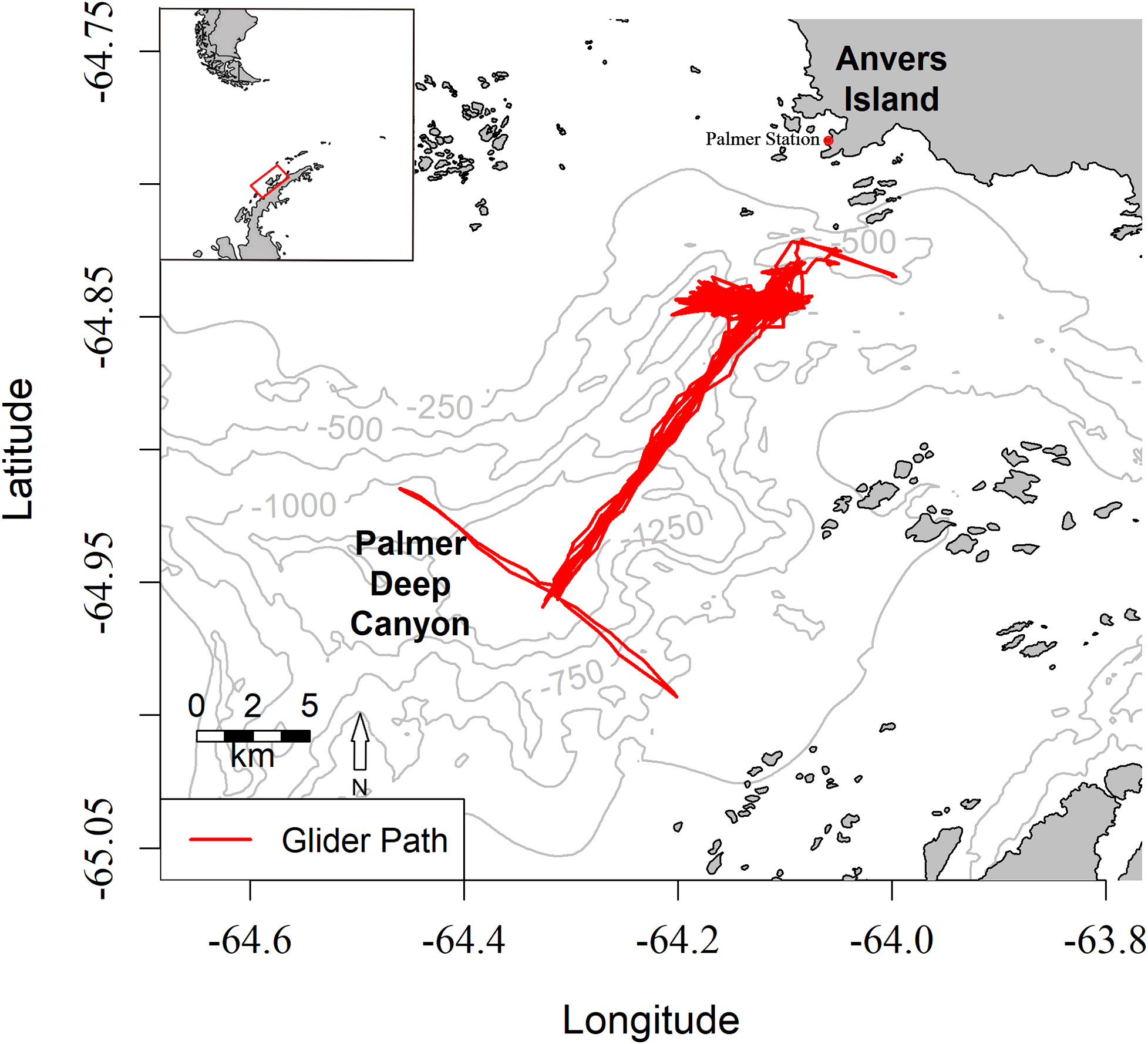
Figure 1 Map of survey area at Palmer Deep Canyon with tracks of the Slocum glider in red. Palmer Station on Anvers Island is marked with a red dot. Grey isoclines depict canyon bathymetry. The Western Antarctic Peninsula is visible in the inset with the red box illustrating the location of the survey area.

2.2 Validation of salp target strength thresholds with ground truthing surveys

Several target strength (TS) thresholds have been empirically derived from in situ and laboratory acoustic analyses of salps in the Southern Ocean (Table 1). However, many do not account for TS overlap with other prevalent zooplankton species, including Antarctic krill (TS ranges from -70 dB to -30 dB). To conservatively assess salp presence using acoustics during our study, it was important to first validate salp TS using ground truthing surveys. To account for potential overlap with Antarctic krill TS thresholds, we used salp TS thresholds of -85 dB to -70 dB (Woodd-Walker et al., 2003; Tarling et al., 2009; Wiebe et al., 2010; Guihen et al., 2014; Tarling et al., 2018). This approach was particularly effective during our study because salps were anomalously abundant and krill were scarce.

TABLE 1

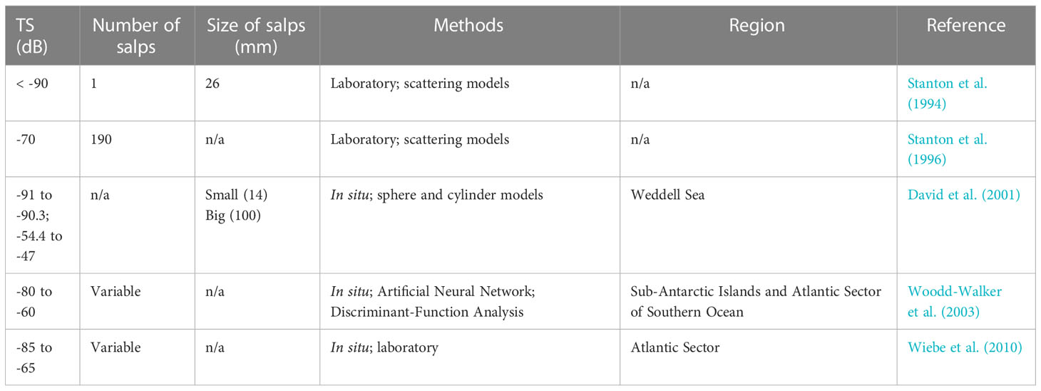
Table 1 Target strengths (TS; dB), details on number of salps, size of salps (mm where numbers are given), study methods, and study regions of referenced past work that acoustically analyzed salps in the Southern Ocean.

For the ground truthing and validation, we used a hull-mounted SIMRAD EK80 single-beam, single frequency (120 kHz) echosounder (Kongsberg Maritime) aboard the RV Hadar, from which we simultaneously sampled zooplankton with nets and net-mounted video cameras. We sampled zooplankton using either a 1 m² metro net fitted with 700 µm mesh or a 1 m² ring net fitted with 200 µm mesh, both deployed from the A-frame aboard the RV Hadar. The hull-mounted EK80 echosounder was configured with a 1 s ping rate, 512 µs pulse duration, and 24 µs sampling duration. We calibrated the EK80 during the season with a tungsten sphere (diameter = 38.1 mm). Visualization of the acoustic data in real-time was achieved with an onboard computer equipped with SIMRAD EK80 software allowing us to conduct targeted net tows to identify acoustic scatterers. Additionally, calibration of data was performed post-sampling through incorporation of data from the onboard CTD.

In addition to targeted net tows, we deployed nets obliquely from the surface to 50 m at two predetermined stations. Contents of the nets were carefully removed and set aside for later analyses in the Palmer Station laboratory. Both nets were equipped with Star-Oddi DST depth loggers. In the laboratory, salps were identified to species level and life stage, and enumerated. Up to 100 individuals per species, stage, and catch were randomly selected for length measurements (oral-atrial length; Foxton, 1966; Supplementary Figure 1). During two RV Hadar surveys (12 net tows in total), a CATS camera (Customize Animal Tracking Solutions) was attached to the metro net to record the presence of organisms in the net path. Video footage was processed in 1 frame per second (fps) periods using Adobe Premier Pro with presence/absence of salps noted. Using date, time, and water column position from the Star-Oddi, we synchronized net contents and video footage with EK80 acoustic data from those two survey days.

Acoustic data from the EK80 echosounder were processed using Myriax Echoview software version 11.1 following Woodd-Walker et al. (2003) and Wiebe et al. (2010) for salps and Tarling et al. (2009); Tarling et al. (2018) for krill. Initial processing of raw acoustic data included calculating the relevant speed of sound and absorption coefficient from the onboard CTD values, along with removing background noise and other interferences. This was done by applying the Background Noise Removal (De Robertis and Higginbottom, 2007) and Impulse Noise Removal (Ryan et al., 2015) algorithms in Echoview. Echograms were parameterized, and groups of salps were identified using a range of target strength (TS) thresholds of -85 dB to -70 dB, while krill were detected using a TS threshold of -70 dB to -30 dB (Tarling et al., 2009; Guihen et al., 2014; Tarling et al., 2018) in the Schools module of Echoview following similar protocols developed by other research groups that have acoustically assessed Antarctic zooplankton in coastal waters (Nardelli et al., 2021; Reiss et al., 2021).

To confirm that the above TS thresholds were correctly identifying salps and not misidentifying krill as salps, we matched known salp and krill occurrences measured either with nets or video footage to acoustically detected groups of salps and aggregations of krill. Collectively, 101 net tows were performed with corresponding acoustic data and net contents. Twelve of those tows also had synchronous video footage. Given the range of TS thresholds that have been derived for salps (Table 1), visually matching our acoustic data to known groups of salps allowed us to explore salp TS ranges more, thus fine-tuning our techniques. We used Mann-Whitney U tests to assess differences in aggregation morphology (area and length) and backscattering energy (S_v and Nautical Area Scattering Coefficient, NASC) between the acoustically identified salps and krill (Woodd-Walker et al., 2003; Table 2). Because of the significant differences in the morphology and backscattering energy of the acoustically identified salps and krill (Table 2), and the validation of our TS thresholds using net tows and video footage (Supplementary Figures 2, 3), we are confident in our identification of salps from the acoustic data collected during this study. The reduced acoustic noise in the glider-borne AZFP data and the overall reduced presence of krill compared to salps were also advantageous to this work.

TABLE 2

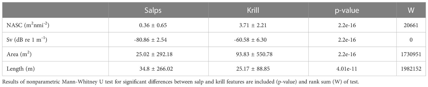
Table 2 Mean ± SD of Nautical Area Scattering Coefficient (NASC; m²nmi^-2; values per organism group not PRC NASC), volume backscattering strength (Sv; dB re 1 m^-1), area (m²), and length (m) of detected salp groups and krill aggregations.

2.3 Data processing of the glider-borne AZFP

Acoustic data from the AZFP echosounder were processed as described above using Myriax Echoview software version 11.1. Although the glider-borne AZFP was equipped with multiple frequency transducers, our ground truthing and TS threshold validation was done with a single frequency (120 kHz) transducer. For this reason, we have only used data from the 120 kHz transducer of the AZFP. Nonetheless, this frequency is commonly used in zooplankton assessments (e.g., Stanton et al., 1996; Brierley et al., 1998; Lawson et al., 2004; Wiebe et al., 2010) and, given the predominance of salps over any other potential scatterers during our survey, we were confident in its use for our study. Because of the orientation that the AZFP transducer was mounted to the glider, acoustic data were only collected on the downcast of each glider profile when the transducer was facing vertically downward into the water column (Reiss et al., 2021). We pre-processed raw acoustic data from the AZFP, by removing background noise and other interferences. Given the previously identified acoustic signals of salps (Table 1), signal to noise ratio was set to -96 dB to prevent misidentification of background noise as salps. Following protocols from Taylor and Lembke (2017), the maximum range of detection from the AZFP was set to 70 m. To avoid interference from the seafloor and surface, both regions were first detected using Echoview’s automatic detection features and then manually reviewed to prevent misidentification. Data within 5 m of the surface and seafloor were also removed to reduce further interference. As before, echograms were parameterized and groups of salps were identified using the TS threshold selected in our ground truthing and validation: -85 dB to -70 dB. All acoustically detected groups of salps were manually reviewed before any subsequent analyses. Acoustic data were then exported in gridded 5-by-5 m cells. For each 5-by-5 m cell where salps were present the proportioned salp region to cell NASC value (often referenced as PRC NASC; hereafter simply called NASC) was calculated in Echoview and exported for the analyses described below. NASC values are a common proxy for organism presence via acoustic measurements. Values for mean depth (m), date, and time per cell were also exported.

We merged mean salp NASC values with the glider downcast data by matching the two datasets at the closest depth in the water column and nearest time (Figure 2). We then integrated mean salp NASC values for each dive profile across the top 500 m of the water column and refer to this in subsequent analyses as Int500. Using temperature and salinity measurements made by the glider CTD, we identified water masses following Carvalho et al. (2016) and Hudson et al. (2019) (Table 3). These water masses were consequently assigned to each mean salp NASC value on each profile. For each dive profile, we calculated mean salp NASC values of each water mass identified on that dive and calculated daily means for each water mass. Temperature profile data collected by the glider were used to establish three distinct regimes during our study (1) early season, (2) mid-season, and (3) late season (Figure 3) and each dive profile of the glider was assigned to a regime.

FIGURE 2

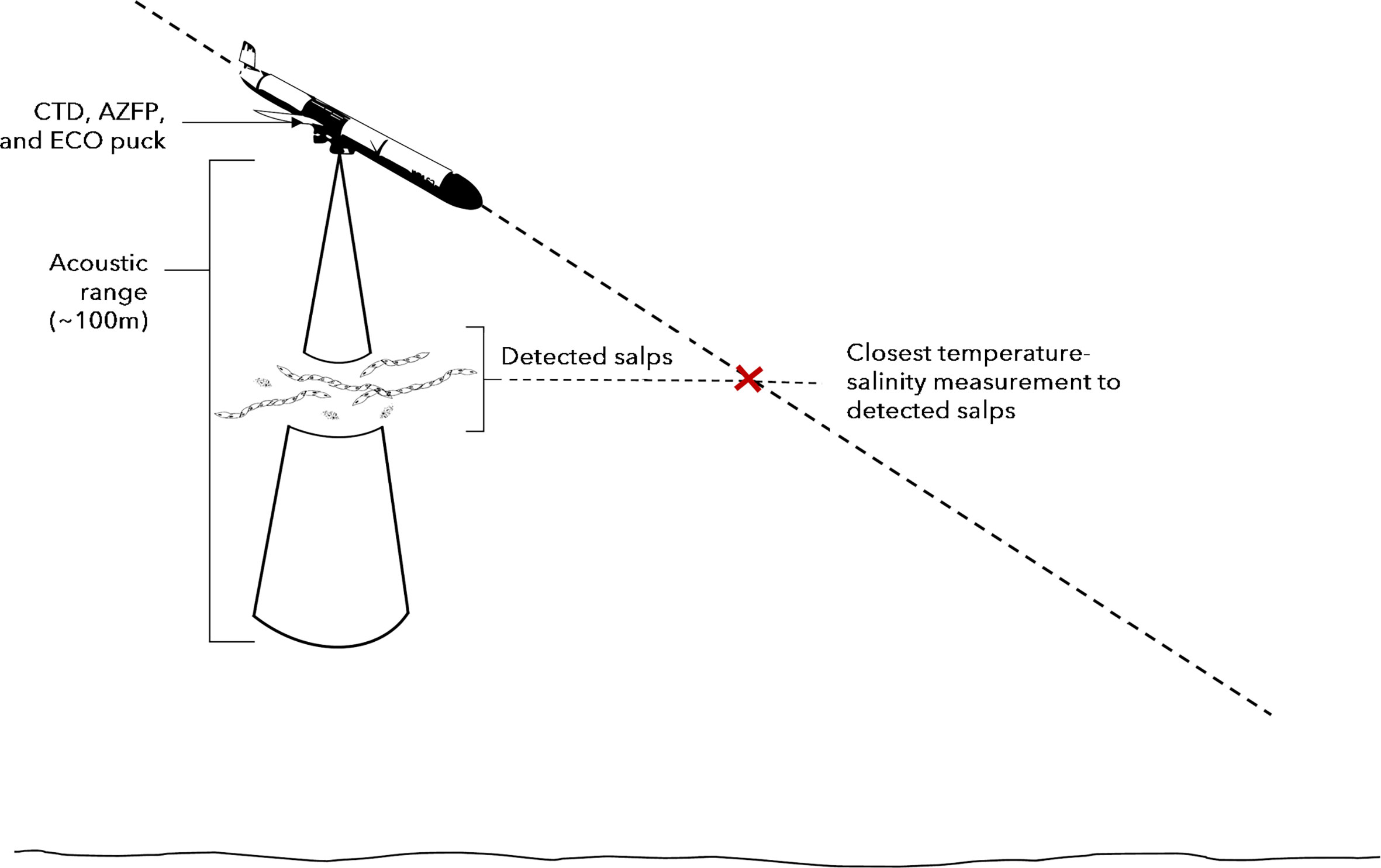
Figure 2 Illustration of method used to associate acoustically detected groups of salps with closest temperature and salinity measurements from glider-borne CTD.

TABLE 3

Table 3 Water mass features (temperature and salinity) during glider deployment.

FIGURE 3

Figure 3 Temperature (°C, top panel), salinity (middle panel), and chl-a (µg L^-1, bottom panel) profiles obtained within the top 500 m of the water from glider-borne sensors between January 11^th and March 9^th, 2020. Dashed black lines in each panel represent the transition date between early and mid-season. Dotted black lines in each panel represent the transition date between mid- and late season.

We associated salp NASC data (collected on the glider downcast) with closest available chl-a data (collected on the glider upcast). This was done for each glider dive profile by integrating chl-a and salp NASC across 50-m depth bins over the top 500 m the water column and matching each by depth and profile. We refer to these integrated values as ChlInt50. To examine diel vertical migration (DVM) in salps, we integrated mean salp NASC for each dive profile across the top 50 m and 150 m of the water column, we refer to these values as IntTop50 and IntTop150, respectively. For each profile, ChlInt50, IntTop50, and IntTop150 were then assigned to either “day” or “night” by determining sunrise-sunset times using local time and geographic coordinates according to Beauducel (2021) in MATLAB (2020).

2.4 Data analyses

Prior to statistical analyses, we used the Shapiro Wilk method to determine that mean salp NASC, Int500, and ChlInt50 were not normally distributed and did not have equal variance, and consequently used non-parametric tests for our analyses. Because the sampling location was extended in the latter part of the season, we first used a Kruskal-Wallis test to determine if there were any significant differences in mean salp NASC between the station-keeping position and the cross-canyon transect. After finding that there were no significant differences in mean salp NASC between the two regions (chi-squared = 0.2, p = 0.6547), the data were pooled and analyzed together in all subsequent analyses.

To test whether the changes to the physical properties of the water column observed throughout the season altered the salp NASC significantly, we compared Int500 between the three regimes (early season, mid-season, and late season) using a Kruskal-Wallis test followed by a Dunn’s post-hoc test and Benjamini-Hochberg adjustment. Then, we compared daily means of salp NASC between water masses for each regime and then between regimes for each water mass using Kruskal-Wallis tests followed by Dunn’s post-hoc tests with Benjamini-Hochberg adjustment. To determine whether salps were undergoing DVM during our study, we calculated, for each regime, night:day ratios of IntTop50 and IntTop150 following the approach of Conroy et al. (2020). ND50 refers to the night:day ratio of IntTop50, while ND150 refers to that of IntTop150. Larger values of ND50 than ND150 indicate shallower occurrences during the night. Values > 1 indicate that salp NASC was higher in the night than in the day at that depth. To determine if there was a relationship between salp NASC and chl-a, we ran a Pearson’s correlation analysis on log-transformed daily means of ChlInt50 for salp NASC and chl-a. All analyses were performed in R Version 1.3.1093.

3 Results

3.1 Oceanographic features

Through the season, the physical properties of the water column showed three distinct regimes that we refer to here as (1) early season, (2) mid-season, and (3) late season (Figure 3). The early season was characterized by the presence of a remnant Winter Water (WW) layer. The mid-season was marked by the breakdown of the remnant WW layer, enhanced mixing of the upper water column, and the deepening of the warm surface layer. By the late season, a freshwater lens had appeared at the surface and a colder water mass had developed between about 50 and 180 m depth (Figure 4).

FIGURE 4

Figure 4 Temperature-salinity plots from the (A) early, (B) mid, and (C) late season regimes with colors representing depth and previously defined water masses outlined (Antarctic Surface Water, AASW; Winter Water, WW; and modified Upper Circumpolar Deep Water, mUCDW).

During our study, temperature ranged from -1.14 to 3.53 °C while salinity ranged from 32.21 to 34.69. Using temperature-salinity definitions of local water masses, we identified Antarctic Surface Water (AASW), modified Upper Circumpolar Deep Water (mUCDW), and remnant WW, but no Upper Circumpolar Deep Water (UCDW) (Figure 4). Two additional water masses were also detected but did not meet any other prior parameterization for the region (Table 3). The first of these was a water mass indicative of mixing between the summer AASW, mUCDW, and the remnant WW, we refer to this here as “other”. The “other” water mass warmed through the season as the remnant WW layer was broken down due to mixing and solar radiation warmed the surface waters. The second additional water mass was a freshwater (FW) lens, that was observed at the surface. Across the three regimes, we observed a deepening of the AASW layer from a minimum of surface to 25 m, surface to 40 m, and surface to 55 m in the early, mid, and late seasons, respectively. The remnant WW layer was only observed in the early season and extended from 61 to 90 m depth. The upper-most depth of mUCDW increased from 53 m in the early season to 61 m in the late season. The surface FW lens deepened from a maximum depth of 7 m in the mid-season to a maximum of 17 m in the late season. mUCDW and “other” water were present every day of the survey, while AASW was observed 80% of the time, the FW lens 20% of the time, and remnant WW only noted 5% of the time.

3.2 The presence of salps: Temporal variability and association with water masses

In the 5-by-5 m bins where salps were detected, raw acoustic backscatter signals ranged from -71.40 to -98.97 dB re 1 m² m^-2 with a mean value of -81.45 dB re 1 m² m^-2 (Supplementary Figure 4). NASC values ranged from 0.0001 to 6.55 m² nmi^-2 with a mean value of 0.1399 m² nmi^-2. Those measurements spanned salinities of 32.21 to 34.68 and temperatures of -1.03 to 3.37 °C. Daily mean integrated salp NASC was similar in the mid and late season regimes (p = 0.23), and significantly higher during the later regimes than earlier in the season (p < 0.001 in both cases, Figure 5).

FIGURE 5

Figure 5 Mean integrated salp NASC (calculated from integrated PRC NASC over the top 500 m) between the (1) early, (2) mid, and (3) late season regimes. Lowercase letters represent significant differences between season regimes.

In the early season, mean salp NASC was significantly higher in AASW (mean = 0.012 m² nmi^-2, SD = 0.009 m² nmi^-2) and the “other” water mass (mean = 0.002 m² nmi^-2, SD = 0.002 m² nmi^-2) than in either the mUCDW (mean = 0.0002 m² nmi^-2, SD = 0.0002 m² nmi^-2p < 0.05) or the remnant WW (mean = 0 m² nmi^-2, SD = 0 m² nmi^-2, p < 0.05, Figure 6). As the survey progressed into the mid-season regime, mean salp NASC was significantly higher in AASW (mean = 0.014 m² nmi^-2, SD = 0.009 m² nmi^-2) and the FW lens (mean = 0.033 m² nmi^-2, SD = 0.033 m² nmi^-2) than in the “other” water mass (mean = 0.003 m² nmi^-2, SD = 0.004 m² nmi^-2, p < 0.05, Figure 6). Lowest mean salp NASC in the mid-season was found in mUCDW (mean = 0.0003 m² nmi^-2, SD = 0.0002 m² nmi^-2, p < 0.05, Figure 6). By the late season, mean salp NASC in both the mUCDW (mean = 0.0005 m² nmi^-2, SD = 0.002 m² nmi^-2) and “other” water mass (mean = 0.0008 m² nmi^-2, SD = 0.0004 m² nmi^-2) was significantly lower than that in either the AASW (mean = 0.009 m² nmi^-2, SD = 0.007 m² nmi^-2, p > 0.05) or the FW lens (mean = 0.015 m² nmi^-2, SD = 0.008 m² nmi^-2, p > 0.05, Figure 6).

FIGURE 6

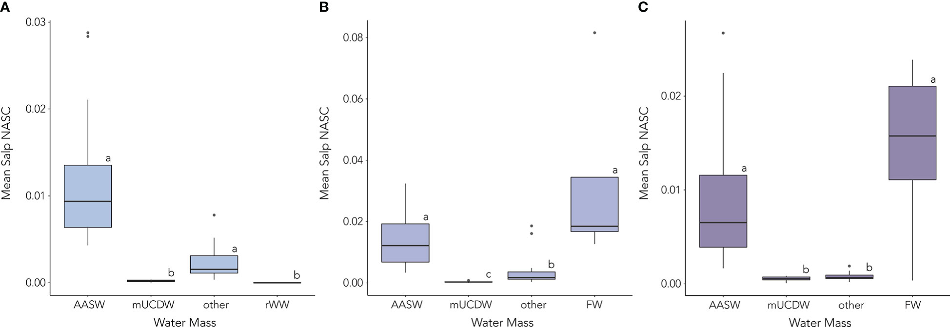
Figure 6 Mean integrated salp NASC (calculated from integrated PRC NASC per water mass for each profile) per present water masses during the (A) early, (B) mid, and (C) late season regimes. Water masses included Antarctic Surface Water (AASW), modified Upper Circumpolar Deep Water (mUCDW), an unidentified water mass (other), the Freshwater lens (FW), and remnant Winter Water (rWW). Lowercase letters represent significant differences between water masses.

Within AASW, mean salp NASC showed no significant change between the three regimes (p > 0.05). However, mean salp NASC in the “other” water mass decreased significantly from the early and mid-seasons to the late season (p < 0.001 in both cases). In the mUCDW, there was a significant increase in mean salp NASC from early to mid-season (p < 0.05) and again from mid to late season (p < 0.05). There was no significant change in mean salp NASC in the FW lens between the mid and late season.

3.3 Vertical distribution and DVM of salps

During our survey, salps were found throughout the water column from the surface to 990 m. To account for reduced sampling at greater depths (the glider spent 75% of its station-keeping deployment in waters above ~400 m with an AZFP range of 100 m below that, meaning that the upper 500 m of the water column was sampled most frequently), only data from depths shallower than 500 m were used in our analyses of vertical distribution. Highest salp NASC integrated by 50 m bins (i.e., ChlInt50) was observed in shallower waters from 0 to 50 m across the season (Figure 7). Median night:day ratios were <1 at the 50 and 150 m depth increments (i.e., ND50 and ND150, respectively) in the early season (Table 4), implying that mean integrated salp NASC values in surface waters were not higher at night than during the day. However, by mid-season, median ND50 and ND150 were marginally >1 (Table 4), indicative that salps may have been undergoing DVM. Median ND50 dropped < 1 and ND150 remained near 1 in the late season (Table 4). Highest ND50 and ND150 were seen in the mid-season regime where maximum values reached 10.36 and 7.81, respectively (Table 4).

FIGURE 7

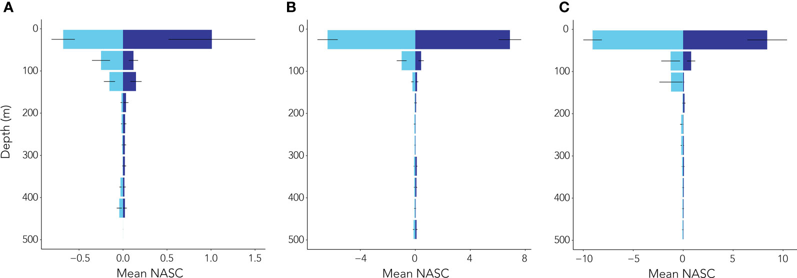
Figure 7 Mean ± standard error of integrated salp NASC day: night ratios (calculated from integrated PRC NASC per profile and time of day) detected from the surface to 500 m depth in 50 m depth intervals during the (A) early, (B) mid, and (C) late seasons. Light blue bars denote daytime periods while dark blue denote night time periods.

TABLE 4

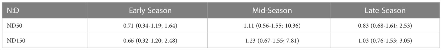
Table 4 Median (25^th and 75^th quantiles; maximum) of night:day ratios of integrated salp NASC (calculated from integrated PRC NASC) in the top 50 m (ND50) and top 150 m (ND150) of the water column during the early, mid, and late seasons.

3.4 Correlation between Chl-a and Salp NASC

Chl-a ranged from 0 to 6.83 µg L^-1 throughout the season, with highest chl-a concentrations in the upper 50 m of the water column. Chl-a integrated over the top 200 m varied throughout the season. A Kruskal-Wallis test and post-hoc Dunn’s test with Benjamini-Hochberg adjustment revealed that integrated chl-a increased significantly from the early season (mean = 248.89 mg m^-2) to the mid-season (mean = 288.60 mg m^-2, p < 0.001), and from the mid-season to the late season (mean = 367.80 mg m^-2, p < 0.001, Figure 3). A significant positive correlation was observed between log-transformed chl-a and log-transformed integrated salp NASC (Pearson’s correlation, rho=0.69, p<0.001, Figure 8).

FIGURE 8

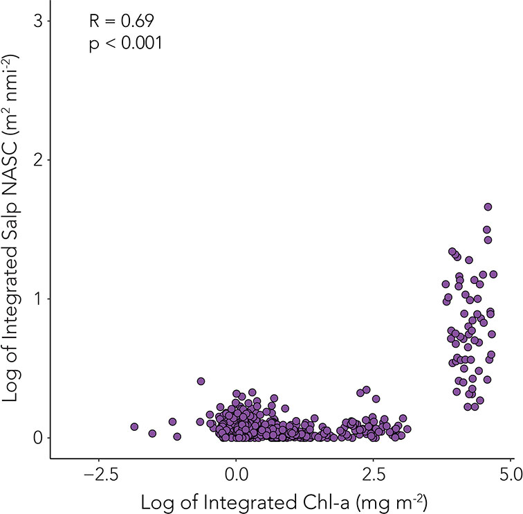
Figure 8 Integrated chl-a (mg m^-2) in 50 m intervals in the top 500 m per profile (from glider upcasts) matched with closest integrated mean NASC (calculated from integrated PRC NASC per downcast profile in 50 m intervals). Only values from glider upcasts and downcasts from the same profile are depicted. Integrated chl-a and mean NASC values were log transformed and Pearson’s correlation was performed on the log transformed values to assess significant correlation. Rho (R) and p-value are provided.

4 Discussion

Using glider-borne acoustics, we have provided new insights into salp vertical distributions and their association with key Southern Ocean water masses by making the first, to our knowledge, high-resolution spatial and temporal measurements of salps in Antarctica. Our survey, conducted in the austral summer (January-March) of 2020, took advantage of an anomalously high salp year at PDC off Anvers Island in the WAP.

4.1 Oceanographic features

During our study, the water column was initially stratified by the presence of a remnant WW layer (temperature minimum = -1.14 ˚C) between 61 and 90 m depth. By January 28^th, however, a strong mixing event caused by persistent high winds from January 25^th to 28^th, with maximum sustained wind speeds of 27.6 knots on January 27^th, resulted in the breakdown of the remnant WW layer. We refer here to the period prior to the breakdown of the remnant WW layer as the early season regime. During the early season, four distinct water masses were identified: AASW, mUCDW, remnant WW, and a water mass referred to here as “other” that likely represented mixing between AASW, remnant WW and mUCDW. Between January 28^th and February 22^nd, referred to here as the mid-season regime, the water column was predominantly well-mixed though the presence of a colder water layer (temperature minimum = -0.08 ˚C) was observed that coincided with the occurrence of an ephemeral FW lens at the surface reaching down to approximately 7 m depth. The mid-season was also marked by a deepening of both AASW and the “other” water mass. By February 23^rd, there was another clear shift in the water column characteristics, and we refer to the regime from February 23^rd to the end of the survey (March 11^th) as late season. In the late season, the FW lens was consistently present, extending down to a maximum of 17 m depth, and a late season phytoplankton bloom had formed. There was no sea ice present during our survey, and the FW lens was most likely caused by freshwater input from glacial calving and melt. In addition, both the AASW and “other” water mass extended deeper into the water column compared to the early and mid-season regimes.

4.2 Seasonal variability in salp densities and association with water masses

Salps were abundant and frequently encountered during our glider survey of PDC. Salp densities (using NASC as a proxy) increased through the season, with the initial significant increase occurring following the breakdown of the remnant WW layer, as described above. In the early season, mean salp NASC was significantly higher in both AASW and the “other” water mass than in either the mUCDW or the remnant WW layer. In fact, the remnant WW layer was devoid of any salps at all, with a NASC of zero. WW is a cold, salty water mass formed by the rapid cooling of surface waters during the winter. In summer along the WAP, WW can be found above the permanent pycnocline at ~ 150 m depth (Mosby, 1934; Martinson et al., 2008) typically lying between the AASW and mUCDW (Smith et al., 1999). At PDC, Carvalho et al. (2016) observed WW at depths shallower than 100 m. Often, seasonal heating and mixing with AASW and mUCDW in summer reduces WW layers and only remnant WW remains. During the summer, and depending on annual conditions, remnant WW can be completely absent, or it can persist in thinner layers at depths of 50 – 100 m (Hofmann and Klinck, 1998; Smith et al., 1999), which is what we observed in the early season of our survey. When cold water layers (like WW) are present, salps are unable to cross the thermal barrier through vertical migration and remain concentrated either beneath or above the layer (Pakhomov, 1993; Pakhomov, 1994). This has been observed near Mordvinov Island (also known as Elephant Island) and Bransfield Strait (West Antarctica; Pakhomov, 1994), and Lützow-Holm Bay (East Antarctica; Ono and Moteki, 2013) and our data corroborate those findings.

During the mid-season regime, we observed an increase in overall integrated salp NASC (Int500). Since there was no significant increase in mean salp NASC in either the AASW or “other” water mass, but an increase in salps in mUCDW, it is plausible that the overall increased salp NASC we observed in the mid-season was due to influx of salps through advection of mUCDW into the study area. UCDW and mUCDW play an important role in salp advection into coastal waters and are key water masses for salp overwintering (Foxton, 1966; Lancraft et al., 1991; Pakhomov et al., 2006; Pakhomov et al., 2011). Relatively warm, salty UCDW (1.7 ≥ temperature ≤ 2.13 °C, 34.54 ≥ salinity ≤ 34.75; Martinson et al., 2008) originating from the Antarctic Circumpolar Current-core (ACC-core) is upwelled at the Antarctic Divergence and may be advected onto the shelf and towards the coast by deep bathymetric features, including canyons like PDC (Hofmann and Klinck, 1998; Klinck et al., 2004; Couto et al., 2017). As the UCDW moves inshore, it mixes with cooler, shallow coastal waters and forms mUCDW (0 ≥ temperature ≤ 1 °C, 34.1 ≥ salinity ≤ 34.7) situated at depths of between 200 and 800 m (Smith et al., 1999; Klinck et al., 2004; Martinson et al., 2008). The warmer UCDW is thought to be ideal for overwintering small, solitary salps that perpetuate the population through rapid asexual reproduction under favorable environmental conditions in the spring and summer (Casareto and Nemoto, 1986; Pakhomov et al., 2002; Henschke et al., 2021a). Consequently, it is likely that the intrusions of UCDW onto the Antarctic shelf carry a seed stock for coastal salp populations (Pakhomov et al., 2006; Pakhomov et al., 2011; Groeneveld et al., 2020). We speculate that the presence of favorable conditions during our 2020 field season, and increase in favorable conditions as the season progressed, may have prompted rapid local population growth of this seed stock.

By the late season, integrated salp NASC (Int500) had not increased significantly, but we observed a shift in the distribution of salps within the water masses. Mean salp NASC was significantly higher in mUCDW and lower in the “other” water mass than it had been in the mid-season. Despite these small changes, the majority of salps were still in the surface waters either in the AASW or the FW lens. Given the historic association of salps with temperate-polar oceanic conditions (Foxton, 1966), the warmer AASW and FW lens may have provided preferable thermal conditions for salps to persist and reproduce in. Both water masses also occupied the upper portion of the photic zone in which chl-a was highest (discussed in more detail below).

4.3 Vertical distribution and DVM of salps

Salps were found throughout the water column with highest depth-integrated mean NASC in the surface waters from 0 – 50 m during all three regimes of our survey. The observed vertical distribution of salps during our study may represent associations with water masses (as described in section 4.2) as the peak in mean depth-integrated salp NASC aligns with depths at which AASW and FW lens were present. In addition, the upper photic zone was the region of highest chl-a concentrations and salps may have preferentially remained in that layer to feed on phytoplankton. Indeed, food availability in the form of phytoplankton is thought to drive vertical distribution patterns of salp populations. Nishikawa and Tsuda (2001) attributed the concentration of salps in shallow depths (30 – 120 m) to the prevalence of phytoplankton in the photic zone. During our survey, we found that there was a positive correlation between chl-a and salp NASC. Further, the depth range of our distribution peak aligned with that of the chl-a maximum identified from the glider’s measurements during our survey as well as the common depth for chl-a maximums in the summer at the WAP (Clarke et al., 2008; Trimborn et al., 2015; Carvalho et al., 2016; Conroy et al., 2020).

In the early season, median night:day ratios of salp NASC integrated over the top 50 and 150 m (ND50 and ND150, respectively) were < 1, indicating that salps were not undergoing diel vertical migration (DVM). In contrast, during the mid-season regime, median ND50 and ND150 were >1, which is indicative of DVM. While our median ND50 of 1.11 is similar to that observed for salps across the same depth range by Conroy et al. (2020), ND50 = 1.2) over the continental slope along the WAP, the median ND150 of 9 observed for salps by Conroy et al. (2020) is substantially higher than our value of 1.23. Furthermore, the 75^th quantiles for ND50 (6.5) and ND150 (9) presented by Conroy et al. (2020) are higher than our values of 1.54 and 1.55, respectively. These comparisons suggest that while salps during our study may have been undergoing some degree of DVM, this trend was weak. While DVM by salps has been observed by other researchers around Antarctica (e.g., Perissinotto and Pakhomov, 1998b; Conroy et al., 2020; Henschke et al., 2021b), some studies have observed a complete lack of DVM by salps (e.g., Nishikawa et al., 1995) suggesting our findings of relatively insignificant DVM are not unusual. During the early season, ND50 was greater than ND150, suggesting salps were more prevalent in the top 50 m at night. By the mid- and late seasons, ND50 was lower than ND150, indicating that salps were prevalent throughout the top 150 m at night.

There are several possible reasons for the observed seasonal shift in salp vertical distributions and patterns of DVM. The first shift, from lack of DVM in the early season to marginal DVM in the mid-season was possibly caused by the mid-season breakdown of the remnant WW layer and enhanced mixing in the upper water column, which may have facilitated the vertical movement of salps. Indeed, studies have found that when temperature gradients are reduced, for instance through strong mixing events, the vertical migration of salps is no longer restricted (Perissinotto and Pakhomov, 1998a; Perissinotto and Pakhomov, 1998b; Pakhomov et al., 2002; Pakhomov et al., 2011). The elevated nighttime salp NASC in the top 150 m (ND150) in the mid- and late seasons compared to the early season may reflect the deepening of the AASW layer. Another potential cause of the changes in vertical distribution patterns and DVM we observed may have to do with ontogenetic differences in both. For instance, Casareto and Nemoto (1986) and Henschke et al. (2021b) noted size- and stage-specific variability in vertical distribution of salps. Casareto and Nemoto (1986) observed small aggregates and large solitary individuals in shallower waters and vice versa at depth. On the other hand, Henschke et al. (2021b) observed smaller individuals of both stages undergoing DVM while larger, mature individuals remained at depth. Our findings emphasize the need for improved understanding of the vertical distribution patterns of salps and the drivers thereof.

4.4 Possible drivers of high salp prevalence in the summer of 2020

While this study did not attempt to quantify salp abundances, we did detect high salp presence acoustically and with net tows. These observations align with other studies at the northern Antarctic Peninsula that also noted high salp presence in the austral summer of 2019-2020 (E.F. Rombola, 2022, personal communication). Here we discuss two potential drivers of salp bloom development in the summer of 2020: (i) temperature, and (ii) phytoplankton biomass.

Low seawater temperatures are thought to effect salp growth, fertilization rates, and mobility (Chiba et al., 1999; Henschke et al., 2018). In an individual-based model of salps from Groeneveld et al. (2020), temperatures less than -0.5 °C were a limiting factor for increased growth. However, temperatures less than -0.5 °C were not found to increase salp mortality in those models (Groeneveld et al., 2020). Temperature is also thought to affect salp muscle pulsation rates, which control mobility and feeding (Harbison and Campenot, 1979). While no direct measurements of S. thompsoni pulsation rates exist, under ice observations and life cycle models suggest that maximum pulsation occurs between 4 and 5 °C with pulsation rates reduced to 60% in temperatures below -2 °C (Henschke et al., 2018). Our measured seawater temperature range did not cross the suggested optimal temperature range, nor the temperature associated with a 60% reduction in pulsation.

In comparison, at moderately warmer temperatures, salps have been observed to consistently and rapidly reproduce in both solitary and aggregate forms (Chiba et al., 1998; Pakhomov and Hunt, 2017). We observed both solitary and aggregate salps in ground truthing net tows throughout the season. Abundances of smaller solitary individuals and embryos increased in tows later in the season suggesting that they had been recently released (Supplementary Figure 1). Salp communities dominated by small aggregate and solitary stages have been attributed to unfavorable water conditions (Siegel and Harm, 1996; Chiba et al., 1999; Henschke and Pakhomov, 2019). However, we consistently caught salps across a large length range (oral atrial length = 3 – 90 mm aggregate stages, 10 – 130 mm solitary stages), further supporting the presence of preferable seawater temperatures for salp growth and reproduction during our survey.

Phytoplankton concentration is another key driver of salp growth. Optimal food concentrations for most pelagic tunicates are typically low (Alldredge and Madin, 1982). Salps propel themselves through the water column by engulfing large volumes of water at their oral opening and expelling it out of their atrial opening using a series of muscle bands. The engulfed water is filtered through a fine mucous mesh before being expelled and the salp consumes the particles trapped in the mucous. As such, salps are non-selective filter feeders. While this mode of feeding allows salps to rapidly consume particles, it can result in mortality if the feeding net becomes clogged with large particles or high particle concentrations (Madin, 1974). This has been used to explain why high salp densities are often observed in regions with low phytoplankton concentrations (0.3 – 0.6 µg 1^-1) and why salps are less abundant when phytoplankton concentrations exceed 1.5 µg 1^-1 (Nishikawa et al., 1995; Loeb et al., 1997; Chiba et al., 1998; Perissinotto and Pakhomov, 1998b; Nicol et al., 2000; Nishikawa and Tsuda, 2001). However, during our survey, average chl-a concentrations in the top 50 m of the water column (where salps were most prevalent) were relatively high, with maximum values of 6.83 µg L^-1 (mean = 1.44 µg L^-1, SD = 1.00 µg L^-1). The negative association of salps with chl-a has been derived from plankton net collections, which provide only a snapshot in space and time. In contrast, the high temporal resolution of our study suggests that it is possible for salps to be present in high densities in regions with higher chl-a concentrations. Given their exceedingly high grazing rates, salps at bloom densities may exert substantial pressure on phytoplankton standing stocks (Bernard et al., 2012), which may explain why most snapshots find high salp abundances and low chl-a concentrations. While we do not disagree that high phytoplankton concentrations would ultimately cause the salp feeding apparatus to clog, we highlight that it is not unreasonable to expect salp abundances to correlate positively with phytoplankton concentrations. In such cases, it is plausible that salps may be competing with other grazers for food.

4.5 Salps and glider-borne acoustics: Advantages, limitations, and suggestions for the future

The acoustic determination of salp densities from glider-borne echosounders offers numerous advantages over traditional sampling techniques. Salps are particularly patchy and ephemeral and traditional sampling techniques (i.e., net trawls) may either miss the patches entirely, or may garner only a snapshot in space and time. Furthermore, attempts to understand vertical distribution patterns are limited to time-consuming collections made by nets like the MOCNESS (multiple-opening-closing net and environmental sensing system, Wiebe et al., 1985). Due to logistical time constraints at sea, the number of deep-water (> 300 m) net deployments on a given survey is often limited, further restricting our understanding of vertical distribution of salps (and indeed other zooplankton) at depths below 300 m (e.g., Loeb and Santora, 2012; Steinberg et al., 2015; Henschke et al., 2021b). The synchronous collection of acoustic data with net tows offers advantages, particularly for patchy zooplankton like salps (Guihen et al., 2014; Benoit-Bird et al., 2018; Reiss et al., 2021). However, the capacity of hull-mounted echosounders, is limited by ship design and sea-state conditions during a given survey, increasing the chance for misidentification of acoustic targets by introducing an excess of noise (Woodd-Walker et al., 2003; A. Hann, 2020, unpublished data). In addition, the vertical coverage of a typical hull-mounted echosounder is within the range of 100 – 300 m (though greater depths can be achieved with lower frequencies), reducing the ability to sample at greater depths, and it often excludes the upper 0 – 20 m of the water column depending on the location of the echosounder (Stranne et al., 2018; Whitmore et al., 2019). Furthermore, acoustic data collection from hull-mounted echosounders may be more synoptic than net trawls, but correlations to water column properties will be limited to data collected by CTD deployments. In comparison, the use of glider-borne acoustics allows one to sample the biological and physical properties of the water column to greater depths, unhindered by the limitations of noise brought about by ship-based operations.

However, there are limitations to the use of glider-borne acoustics that must be considered. Glider-borne echosounders must be compact and lightweight with reduced power consumption needs, and meeting these conditions requires the echosounder to have limited acoustic capability. For instance, on a glider-borne echosounder the range from the transducer is reduced, as are the dynamic range and Sv resolution (Guihen et al., 2014). Another major limitation of glider-borne acoustics exists for highly motile organisms, like krill and fishes, which may exhibit escape responses to an oncoming glider (Guihen, 2018). However, for organisms like salps that are not fast-moving and do not exhibit an escape response, this is unlikely to be of concern. Target identification remains a challenge in acoustics, particularly for organisms like salps for which TS detection constraints are not well-defined. During our survey, net tows confirmed that salps dominated the water column, allowing us to confidently identify salps from acoustic backscatter. However, in regions where salps are not the dominant scatterer, it will be challenging to identify targets without frequent concurrent net tows. Active acoustic assessments rely on organisms to backscatter sound emitted from the echosounder in distinct, identifiable signals. Often backscattering is reliant on smaller organisms (e.g., krill and forage fishes) forming defined aggregations like swarms or schools, which require self-organization (Allee, 1931; Shaw, 1962; Camazine et al., 2020). Although salps are not capable of self-organization at this level, at bloom concentrations, salps cluster in groups at high enough densities that can be detected using the Schools Detection algorithm in Echoview, as we demonstrated in our ground-truthing on this study. However, at lower abundances, individual salps may not cluster at densities detectable by the Schools Detection algorithm and, in these conditions, another means of detection may be necessary. In addition, the solitary and aggregate stages of salps have been observed to co-exist in the Antarctic, but different stages and sizes produce varied acoustic signals (Stanton et al., 1994; Stanton et al., 1996; David et al., 2001; Wiebe et al., 2010). Such variability may cause the same quantity of salps to display different acoustic backscattering or may result in biased signals based on dominant stage and size. These limitations in acoustic knowledge of salps emphasize the need for continued validation of observed backscatter with concurrent net tows. Further work focusing on salp TS thresholds and improvement of current detection algorithms and parameters will enhance methods for assessing salps acoustically.

5 Conclusions

In the austral summer of 2020, we took advantage of anomalously high salp abundances to conduct a high temporal resolution survey of salp vertical distribution patterns and DVM in coastal Antarctic waters. We found that salps were present throughout the water column, with highest frequencies in the top 50 m, which included the AASW and the FW lens. Following the breakdown of the remnant WW layer in late January 2020, we observed an increase in salp densities throughout the water column and the initiation of marginal DVM that persisted for the remainder of that summer. Through this work, we have demonstrated the potential of glider-borne acoustics in studying salp densities, distribution and DVM and our study contributes to the growing body of work on salp range expansion in Antarctic waters.

Data availability statement

The original contributions presented in the study are included in the article/Supplementary Materials. Further inquiries can be directed to the corresponding author/s.

Author contributions

KSB, JK, MJO and HS conceived the larger project that funded this research while AMH and KSB conceived the salp related research. AMH, JK, MJO, and HS performed the fieldwork. AMH conducted the statistical analyses and KSB contributed to the interpretation of the data. AMH led the writing with all authors contributing to the manuscript. All authors contributed to the article and approved the submitted version.

Funding

This work was supported by the US National Science Foundation Grant No. 1745081 (awarded to KSB), 1745009 (awarded to JK), 1744884 (awarded to MJO), and 1745023 (award that funded HS).

Acknowledgments

We thank the US National Science Foundation and Antarctic Support Contract personnel for their logistical support of this project. We also thank the many students and field assistants who assisted in data collection. Specifically, we would like to thank Deborah Steinberg for allowing us to use her sampling equipment, John Conroy for data collection and zooplankton guidance, Grace Saba for lending her glider system, and Ari Friedlander for lending us his CATS camera system. Finally, we would like to thank the rest of the Palmer Antarctica Long-Term Ecological Research team and the National Oceanic and Atmospheric Administration Antarctic Marine Living Resources group for their advice, suggestions, and collaboration.

Conflict of interest

The authors declare that the research was conducted in the absence of any commercial or financial relationships that could be construed as a potential conflict of interest.

Publisher’s note

All claims expressed in this article are solely those of the authors and do not necessarily represent those of their affiliated organizations, or those of the publisher, the editors and the reviewers. Any product that may be evaluated in this article, or claim that may be made by its manufacturer, is not guaranteed or endorsed by the publisher.

Supplementary material

The Supplementary Material for this article can be found online at: https://www.frontiersin.org/articles/10.3389/fmars.2022.857560/full#supplementary-material

References

Alldredge A. L., Madin L. P. (1982). Pelagic tunicates: Unique herbivores in the marine plankton. BioScience 32, 655–663. doi: 10.2307/1308815