Cross-Shelf Exchange in the Southwestern Atlantic Shelf: Climatology and Extreme Events

The variability and drivers of the cross-shelf exchanges between the Southwestern Atlantic shelf and the open ocean from 30 to 40°S are analyzed using a high-resolution ocean model reanalysis at daily resolution. The model's performance was first evaluated using altimetry data, and independent mooring and hydrographic data collected in the study area. Model transports are in overall good agreement with all other estimates. The record-mean (1993–2018) cross-shore transport is offshore, 2.09 ± 1.60 Sv. 73% of the shelf-open ocean exchange occurs in the vicinity of Brazil-Malvinas Confluence (~38°S) and 20% near 32°S. This outflow is mostly contributed by northward alongshore transport through 40°S (63%) and the remaining by southward transport through 30°S (37%). The cross-shore flow presents weak seasonal variations, with a maximum in austral summer, and high variability at subannual and weekly time scales. The latter is mainly associated with abrupt wind changes generated by synoptic atmospheric systems. Alongshore wind variations set up sea-level changes in the inner shelf which in turn drive large anomalies in the associated geostrophic alongshore flow. The difference in inner shelf sea-level anomalies at 30 and 40°S is a good indicator of cross-shelf exchange at seasonal and shorter time scales. Episodes of extreme offshore transport that reach up to 9.45 Sv and last about 2 days are driven by convergence of these alongshore flows over the shelf. Large exports of shelf waters lead to freshening of the upper open ocean as revealed by in-situ and satellite observations. In contrast, onshore extreme events drive open ocean water intrusions of up to 6.53 Sv and last <4 days. These inflows, particularly the subtropical waters from the Brazil Current, induce a substantial salinification of the outer shelf.

1. Introduction

Continental shelves account for <10% of the global ocean surface, yet they host 20–30% of the ocean's primary production (de Haas et al., 2002) and 90% of the global fish catch (Gattuso et al., 1998). In addition, continental shelves play a key role in the biogeochemical cycling of the ocean due to the continental discharge of organic matter and nutrients. Consequently, 80% of organic carbon is buried in continental shelves (Rabouille et al., 2001; Chen et al., 2003) and these are important sites for denitrification (Christensen et al., 1987; Rabouille et al., 2001). The Southwestern Atlantic Shelf (SWAS) hosts one of the most productive marine ecosystems of the southern hemisphere due to the supply of nutrients from continental discharge, shelf currents, and open ocean sources. The high primary productivity over the shelf and its subsequent fate might have a significant biogeochemical impact on the open ocean.

Bounding the SWAS, the Malvinas Current (MC) flows northeastward carrying relatively low-salinity, cold and nutrient-rich waters from the Antarctic Circumpolar Current. The MC reaches approximately 38°S where it collides with the Brazil Current (BC), which advects warm and salty waters southward (Gordon and Greengrove, 1986, Figure 1). The latitudinal position of the Brazil/Malvinas Confluence (BMC) varies seasonally, shifting southward during the austral fall and northward during the austral spring (Combes and Matano, 2014a). There is also a southward shift of the BMC position in the past decades associated with a longer-term oscillation (Lumpkin and Garzoli, 2011).

FIGURE 1

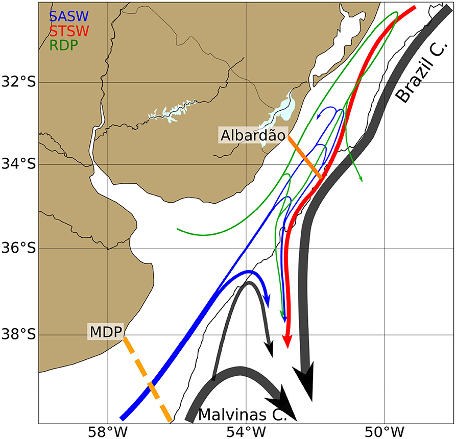
Figure 1. Schematic circulation diagram of the Southwestern Atlantic Shelf between 30 and 40°S. The Mar del Plata (MDP) and Albardão transects are indicated by an orange dashed and solid line, respectively. The gray line indicates the 200 m isobath. SASW, Subantarctic Shelf Water (blue); STSW, Subtropical Shelf Water (red); RDP, Río de la Plata water (green). Adapted from Berden et al. (2020) with permission.

Diluted subantarctic waters referred to as Subantarctic Shelf Waters (SASW) enter the SWAS near 54°S (Piola et al., 2018). These cold, relatively low-salinity (~33.8) and nutrient-rich waters flow northward and reach the Southern Brazilian Shelf at 34°S to 32°S, where they meet a southwestward flow of warm-salty Subtropical Shelf Waters (STSW), forming the Subtropical Shelf Front (STSF, Piola et al., 2000). The STSF is a subsurface front capped by low-salinity waters derived from the Río de la Plata (RDP). The RDP is the major contributor of continental nutrients and organic matter to the central portion of the SWAS (Braga et al., 2008; see Figure 1 in Piola et al., 2018; Bordin et al., 2019; Berden et al., 2020). On average, the RDP discharges around 25,000 m³.s⁻¹ of freshwater over the shelf (Borús et al., 2017). From April to September south of 30°S the continental shelf is dominated by southwesterly winds, while northeasterly winds prevail from October to March (e.g., Matano et al., 2014). These seasonal reversals in alongshore winds have a profound effect on the shelf circulation, leading to northeastward extensions of the RDP low salinity waters to 28°S in fall-winter, and retraction to 32°S en spring-summer (Piola et al., 2000, 2005). Direct current meter observations near 40°S indicate a mean northeastward transport of SASW of 2.65 Sv, with large variability, including transport reversal events lasting a few days, which are closely associated with alongshore winds variability (Lago et al., 2021). Numerical models suggest that the transport over the shelf is modulated by the intensity of the MC, which sets up the cross-shore pressure gradient (Matano et al., 2010). However, altimetry-derived velocity fields and more recent numerical simulations indicate this influence is limited to a few tens of kilometers over the outer shelf (Combes and Matano, 2018; Lago et al., 2021). The influence of the tides north of 39°S is very limited except in the inner portion of the RDP (Palma et al., 2004).

Strong western boundary currents (WBCs), including the BC and the MC, are thought to act as barriers to exchanges between the shelf and the open ocean (Roughan et al., 2011; Franco et al., 2017; Malan et al., 2020). However, in-situ and satellite observations, and numerical simulations indicate that the BMC is an effective conduit of shelf waters toward the deep adjacent ocean (Guerrero et al., 2014; Matano et al., 2014; Berden et al., 2020). Synoptic hydrographic observations suggest that the STSF is nearly density-compensated (Piola et al., 2000, 2008) allowing the necessary baroclinicity for cross-isobaths exchanges (Berden et al., 2020). The slight changes in isopycnal depth on either side of the STSF and its partial cross-shore orientation allow cross-isobath movements suggesting the STSF may be a path of export of shelf waters to the open ocean. Combes et al. (2021) suggest that between 22.2 and 35°S the mean cross-isobath transport is modulated by the bathymetry and its variability is determined by the local wind and the internal variability of the BC. In addition, onshore intrusions of South Atlantic Central Waters (SACW) in the bottom layer of the outer shelf north of the BMC have been reported in several studies (Braga et al., 2008; Möller et al., 2008; Piola et al., 2008; Palma and Matano, 2009; Berden et al., 2020). These SACW intrusions are a significant nutrient source to the shelf region (e.g., Ciotti et al., 1995 and references therein).

Analyses of in-situ observations provided a synoptic characterization of the water exchange between the SWAS and the open ocean (Berden et al., 2020) estimating an offshore transport of 3.44 Sv between 32.1 and 37.7°S. Analyses of altimetry data indicate a maximum off-shelf transport in January–June between 35 and 38°S, and a minimum in July to December (Strub et al., 2015). Matano et al. (2010) and Combes and Matano (2014b) study the interaction between the WBCs and the shelf in the South Brazil Bight and Patagonia based on numerical models. North of 29°S, the circulation is driven by the interaction between intrusions of the BC over the middle and outer-shelf and upwelling favorable wind stress in the inner-shelf. Between 30 and 40°S, the STSF seems to be a preferential path for the ejection of shelf waters. Matano et al. (2014) use 10-day averaged outputs from a high-resolution model (1/24°) to analyze the exchanges of shelf-waters focusing on the sea surface salinity variability. The model suggests that low-salinity waters of the RDP are exported in the vicinity of the BMC. A Lagrangian particle analysis with a similar model indicates that the export of SASW occurs primarily along two different paths (Franco et al., 2018). The waters following a fast path (<2 months) are exported near the BMC and those following a slow path (>130 days), flow northward over the shelf beyond the latitude of the BMC, describe a cyclonic loop near 32°S and subsequently follow the shelf-break southward to the BMC. Likewise, other numerical simulations (1/12°, 10-day average) suggest that the location of the BMC determines the position of the largest offshore transport, but not its magnitude (Combes and Matano, 2018). Recent analyses based on a high-resolution nested model (1/36°, 5-day average) indicate an offshore transport of ~1.6 Sv between 35 and 25.2°S (Combes et al., 2021).

In this article, we extend previous studies analyzing the export of shelf waters to the open ocean between 30 and 40°S and its time and space variability using daily outputs from a global high-resolution ocean model reanalysis. Given the recent observational evidence of large-amplitude alongshore transport fluctuations at a synoptic time scale near 40°S (Lago et al., 2021) we also analyze the model results to determine if such changes may impact the offshore transport. The daily resolution of the reanalysis allows us to study the temporal variability at high frequencies, which has not been discussed hitherto.

2. Data and Methods

2.1. Reanalysis GLOBAL_REANALYSIS_PHY_001_030

This study is based on the analysis of the Copernicus Marine Environment Monitoring Service (CMEMS) global ocean reanalysis (GLORYS12V1) during 1993–2018. GLORYS12V1 is based on the NEMOv3.1 ocean model, described in Madec et al. (2017). The model is driven at the surface by the ERA-interim atmospheric reanalysis from the European Centre for Medium-Range Weather Forecasts. Satellite-derived along-track sea level anomaly (SLA, Pujol et al., 2016), sea surface temperature (SST) from NOAA's Optimum Interpolation Sea Surface temperature (0.25°, Reynolds et al., 2007), sea ice concentration from CERSAT and in situ vertical profiles of temperature (T) and salinity (S) from the CORA4.1 database (Cabanes et al., 2013) are jointly assimilated. The assimilation procedure employs a reduced-order Kalman filter with a 3D multivariate modal decomposition of the background error. The assimilation procedure includes an adaptive-error estimate and a localization algorithm. In addition, a 3D-VAR scheme corrects for the slowly-evolving large-scale biases in temperature and salinity (Lellouche et al., 2018). The reanalysis does not incorporate tidal forcing. The model output is provided daily on a standard regular grid at 1/12° (~8 km) and on 50 standard vertical levels, with 22 levels in the upper 100 m. Consequently, the vertical resolution is 1 m at the surface, decreases to 33 m at the bottom of the continental shelf (200 m), and reaches 450 m near the bottom in the deep ocean (5,700 m).

2.2. In-situ Data

To evaluate the model performance, the model was compared with in-situ data collected during 12 hydrographic surveys over a cross-shelf transect off southern Brazil, hereafter referred to as the Albardão transect (Figure 2 and Table 1). The data consists of high-resolution, cross-shore sections of conductivity-temperature-depth (CTD) profiles occupied between August 2003 and October 2018. In addition, the alongshore volume transport between the coast and the 200 m isobath near 39°S (hereafter referred to as the MDP transect, location shown by the orange dashed line in Figure 1) has been recently estimated, hereafter referred to as T_Obs, based on direct current observations during 11 months from December 2014 to November 2015. Details of these transport estimates are provided in Lago et al. (2021). Note that the in-situ observations used herein were not assimilated to the ocean reanalysis.

FIGURE 2

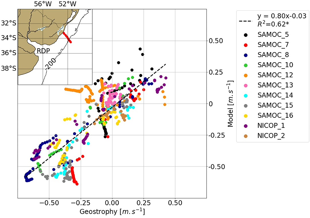
Figure 2. Model vs. geostrophic velocities with a vertical resolution of 10 m during 12 oceanographic surveys over the Albardão section. The dashed line indicates the linear fit to the data. Inset: Location of Albardão transect (red line). The 200 m isobath is indicated by a gray line.

TABLE 1

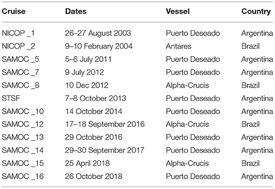
Table 1. Hydrographic surveys along the Albardão transect.

2.3. Satellite Data

The altimetry data (sea level anomalies and associated geostrophic currents) used in this analysis were the delayed-time merged all satellites Global Ocean Gridded SSALTO/DUACS Sea Surface Height L4 product from Copernicus Marine (Pujol et al., 2016). The gridded product has a spatial resolution of 1/4° on a regular grid and a daily temporal resolution.

2.4. Wind Data

Wind stress data was obtained from the ERA5 global atmospheric reanalysis (Hersbach et al., 2020), which covers 1979–2022, produced by the European Center of Middle-range Weather Forecast (ECMWF). This product is available hourly over a regular grid of 1/4°. Daily averages were used in this work.

2.5. Methods

Since the WBCs may act as barriers to exchanges between the shelf and the open ocean, the possible impact of the BC and MC intensity is studied. The analysis of the BC variability is based on the depth-averaged model velocity in the upper 0–200 m at 34.5°S projected in the local along-slope direction (orientation of 36° from the true north). Likewise, the MC velocity was defined at 42°S, where the model velocity is projected to 45° from the true north. Since the BC presents substantial mesoscale variability (see Chidichimo et al., 2021), it is difficult to determine its precise position in the cross-shore direction along 34.5°S in the daily model outputs. Therefore, the position of the current was determined using the mean velocity field between 1993 and 2018 considering the current as a uniform flow with intensity >10 cm.s⁻¹. Once the position of the current is established, the along-slope velocity component is averaged horizontally to obtain a single velocity time series. The same procedure is followed to determine the MC intensity. The sensitivity of the definition of both currents to changes in the velocity threshold and depth over which the velocity is integrated was analyzed (Supplementary Figure 1). The resulting velocity magnitude is not significantly sensitive to changes in depth of integration considering a range of 200–400 m. Although the velocity magnitude displays variations associated with changes in the threshold used to define the BC and MC, tested in the range of 5–20 cm.s⁻¹, these changes are small and the resulting velocities are highly correlated (R²>0.85^*). The significance of the statistical correlations was calculated at a 95% confidence level. Hereafter, significant correlations are indicated with an asterisk (^*), and correlations with R² < 0.15 will not be addressed. In addition, the BMC location was analyzed as a possible driver of cross-shelf exchange. The position of the BMC is determined daily as the latitude where the 10°C isotherm at 200 m intersects the 1,000 m isobath (Goni and Wainer, 2001; Matano et al., 2014).

3. Results and Discussion

3.1. Evaluation of Model Performance

In this section, we evaluate the model's ability to capture the patterns of the shelf circulation and its time variability. To this end, we compare the model outputs with available in-situ and satellite observations.

3.1.1. Currents

The currents extracted from the model over the continental shelf were first compared with in-situ data collected in the Albardão transect (Figure 2). Alongshore geostrophic velocities relative to the sea surface were estimated from the hydrographic data with a vertical resolution of 10 m. Absolute velocities were then computed by adjusting the relative geostrophic profiles to the surface geostrophic velocity derived from the gridded altimetry data. Model velocities were projected in the alongshore direction and low-passed filtered with a 5-day window. Model and observations are in relatively good agreement based on the linear correlation (R² = 0.62^*).

3.1.2. Comparison With Satellite Altimetry

To further evaluate the model performance, we compared the standard deviation of the sea level anomaly (SLA) from the model and the gridded satellite data. It is important to note that the model assimilates altimetry derived along-track sea level. The spatial structures of the standard deviation of SLA (Figure 3) are very similar at offshore locations and present the largest differences over the RDP estuary and coastal regions northeast of the RDP mouth. To analyze the temporal evolution of SLA we selected a location on the mid-shelf close to the climatological latitude of the BMC (36.9°S), which is a preferential location of export of shelf-waters to the open ocean (black dot in Figures 3A,B). The 10-day filtered time series of SLA shows a significant correlation (R² = 0.72^*) between the model and the altimeter data. This correlation decreases considering daily data (R² = 0.50^*) because the model output contains more high-frequency variability than the altimeter data. These differences between altimetry and model results are expected because of the comparatively poor space and time resolution of the altimeter data. Although the gridded altimetry product is available daily, the most frequent (Jason 3) revisits occur at 10-day intervals. Therefore, the gridded altimetric product has an effective spatial and temporal resolution of 280 km and 21 days (see Figures 2B, 3 in Ballarotta et al., 2019) and cannot appropriately resolve estuarine and nearshore features, nor small mesoscale features (Pujol et al., 2016) generated by the model's internal dynamics.

FIGURE 3

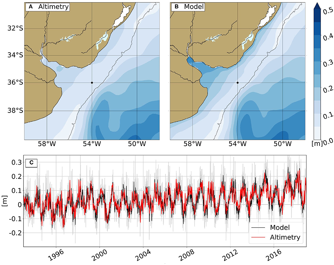
Figure 3. Standard deviation of sea level anomaly based on satellite altimetry (A) and the model (B). The 200 m isobath is indicated by a gray line. (C) Ten-day filtered time series of SLA at 36°S, 54°W (black dot in A,B). Altimetry data is shown in red and model data in black. The daily (unfiltered) model output is shown in gray.

3.1.3. Comparison With in-situ Alongshore Transports

Alongshore transport over the MDP transect between the coast and the 200 m isobath near 39°S was recently estimated by Lago et al. (2021) using in-situ data (T_Obs). The analyses of Lago et al. (2021) reveal the barotropic nature of the circulation and a close agreement between geostrophic and direct transport estimates. To evaluate the model performance, we computed the alongshore component of model transport across the same line, hereafter referred to as T_Model (Figure 4). The time-averaged T_Obs is 2.68 Sv and its standard deviation is 2.13 Sv. Meanwhile, T_Model presents lower mean and standard deviations; 2.13 and 1.32 Sv, respectively. In addition, flow reversal events were analyzed by Lago et al. (2021). Particularly, an event observed in early May 2015 shows a flow reversal from −2.57 to 5.84 Sv in T_Obs and from −1.46 to 5.15 Sv in T_Model.

FIGURE 4

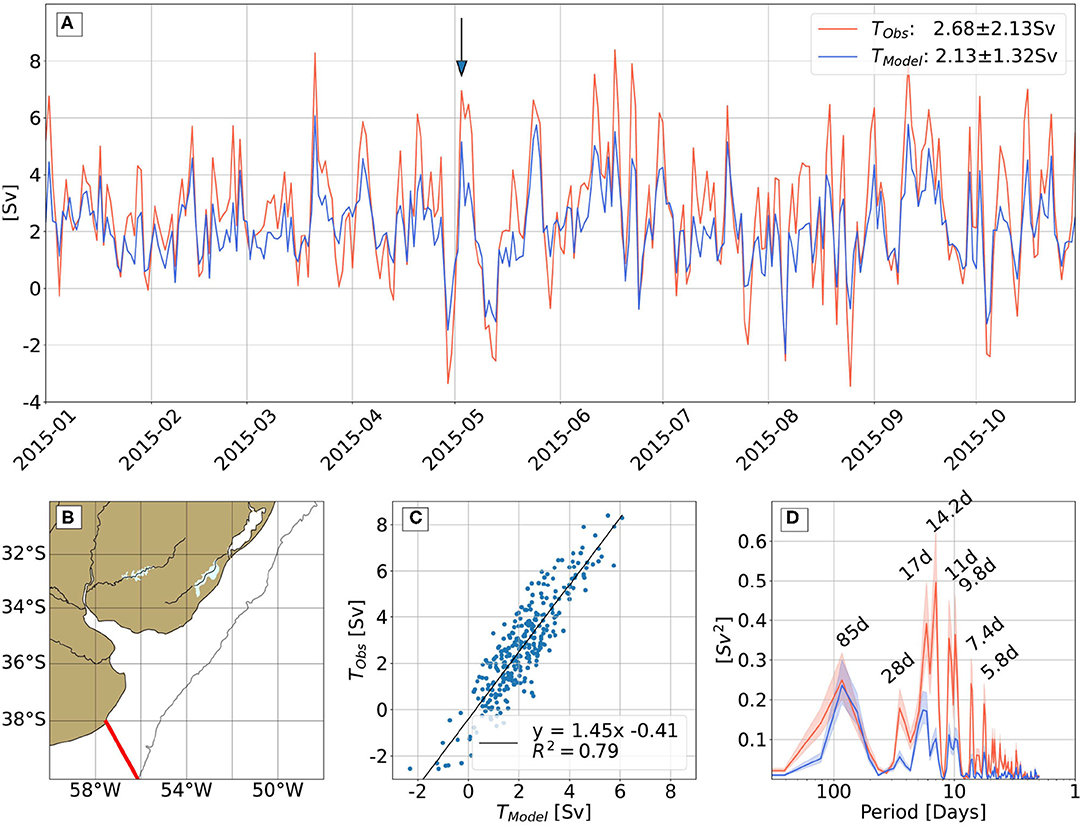
Figure 4. (A) Daily observational (T_Obs, red) and model-derived (T_Model, blue) shelf transport (Sv) across the red line shown in (B). (C) T_Obs vs. T_Model, and linear regression (black line). (D) Power spectrum of T_Obs (red line) and T_Model (blue line) with bands of 95% confidence levels (shadings).

T_Model explains 79% of the variance of T_Obs (Figure 4C). However, the mean difference of 0.55 Sv represents a relative error of 0.55 Sv/2.68 Sv = 0.20, or 20% less than the observed transport. T_Model has less energy than T_Obs, at periods shorter than ~ 30 days. However, both transport time series present peaks at similar frequencies at around 5.8, 7.4, 10, 16, 28, and 85 days (Figure 4D). T_Obs displays higher energy in almost all peaks except at 85 days where both model and in-situ transports are in much better agreement. Hence, the model reproduces the regional dynamics but it contains lower energy at shorter periods.

Additionally, Lago et al. (2021) estimated the alongshore transport using altimeter data (T_Sat). Their mean T_Sat is 2.42 ± 0.64 Sv, thus matching quite well the 2.13 ± 1.32 Sv from the model during the same period. Since the model assimilates along-track altimeter sea level anomaly, this agreement is not surprising.

3.2. Cross-Shore Transport Variability

To study the cross-shore transport between 30 and 40°S and its temporal and spatial variability, the 200 m isobath was divided into 20 zonal bands each spanning 0.5° of latitude (Figure 5). The time-averaged offshore transport through each outer shelf segment was estimated as the sum of the transports entering through the northern and southern boundaries of each zonal band. The total offshore transport between 30 and 40°S, hereafter referred to as T_Cross (Figure 6C), is defined as the sum of the transports entering through the northern boundary at 30°S (T_N, positive southward, i.e., entering the domain; Figure 6A) and the southern boundary at 40°S (T_S, positive entering the domain; Figure 6B). We estimated the changes in the volume of shelf water based on the changes in the model-derived SLA. The resulting rate of daily volume change has a standard deviation of 0.16 Sv, which is an order of magnitude smaller than the typical daily mass convergence between 30 and 40°S. Thus, we assumed the mass storage plays a minor role in the cross-shore transports estimated based on mass conservation. We also investigate extreme events which are defined as those periods when the transport is higher/lower than the record-mean ±2 standard deviations. In addition, possible physical mechanisms modulating the variability of the cross-shore transport such as the intensity of the BC and the MC, the BMC location, the alongshore transport variability, and the winds are analyzed.

FIGURE 5

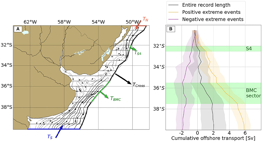
Figure 5. (A) Streamlines over the shelf show time-mean flow structure for the entire record length. Zonal strips used to estimate cross-shore transports (dashed lines). The 200 m isobath is indicated by a heavy black line. (B) Cumulative offshore transport through the 200 m isobath from 30°S across the 20 outer shelf segments. Mean offshore transport during the entire model run period (1993–2018, black), positive (orange, offshore) and negative (purple, onshore) extreme events. The transport standard deviations are indicated by the background shading. The BMC sector and S4 are indicated in green.

FIGURE 6

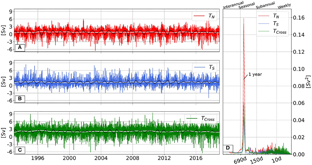
Figure 6. Transports (Sv) over the continental shelf through 30°S (A, red, T_N), 40°S (B, blue, T_S), and cross-shore (C, green, T_Cross). Also shown are T_seasonal plus T_mean (black) and T_interannual plus T_mean (white). (D) Transport power spectra through the same sections. Vertical lines at 10, 150, and 690 days represent the breaks between time scales.

The variability of the shelf transports (T_N, T_S, and T_Cross) can be caused by circulation changes occurring on a variety of time scales. Thus, it is useful to split the model-derived transport variability by filtering the daily transport signals as follows:

$\begin{array}{ll}T=T_{mean}+T_{weekly}+T_{subannual}+T_{seasonal}+T_{interannual}& (1)\end{array}$

where T_mean is the record-mean transport and T_weekly, T_subannual, T_seasonal, and T_interannual are associated with weekly (<10 days), subannual (10 days–5 months), seasonal (5–23 months), and interannual (>23 months) time scales, respectively (Hirschi et al., 2007). To compute each component the daily transport time series is filtered with a Butterworth window of order 5. The weekly scale is included to study the high-frequency variability, which is particularly relevant to understand the extreme offshore transport anomaly events. Table 2 shows the standard deviation of each transport and for each of the above-defined time scales. The larger variability is concentrated on the subannual and weekly time scales, with the latter being the largest. Although the transport power spectrum shows a marked peak around 1 year (2.7–9.2% of energy), there is a substantial amount of energy (>85%) distributed in the high frequencies (subannual and weekly), without a characteristic frequency (Figure 6D).

TABLE 2

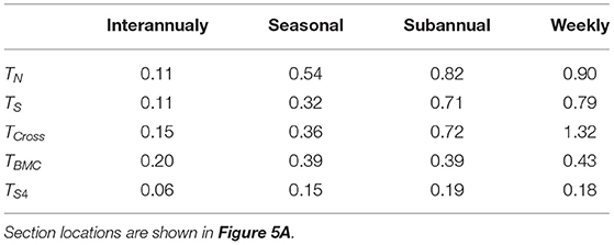
Table 2. Standard deviation of transport (Sv) through selected sections, estimated over the entire model period (1993–2018).

3.2.1. Mean, and Low-Frequency Variability (Interannual and Seasonal)

The record-length mean offshore transport [mean ± 1 standard deviation] between 30 and 40°S (T_Cross) is 2.09 ± 1.60 Sv (Table 3). Sixty-three percent (1.31 ± 1.16 Sv) of T_Cross is contributed by T_S and the remaining 37% (0.78 ± 1.36 Sv) by T_N. The contribution of continental discharge from the RDP is <1% of the offshore transport variability. Previous estimates of the mean off-shelf transport based on the analyses of a high-resolution regional model show a mean offshore transport of 1.21 Sv between 34 and 38°S (Matano et al., 2014). This is in relatively good agreement with the GLORYS12V1 offshore transport computed over the same latitude range (1.72 ± 1.35 Sv).

TABLE 3

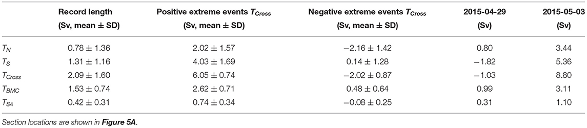
Table 3. Mean transport (Sv) through selected sections for the entire model run (1993–2018), during extreme cross-shore transport events, and during the large transport reversal observed in early May 2015 (see section 4.4).

The offshore flow across the 200 m isobath is not uniform. Most of the flow (1.53 ± 0.74 Sv or 73%, Table 3) occurs in the vicinity of the BMC (between 35.5 and 37.5°S, hereinafter referred to as “BMC sector”) and about 20% of T_Cross occurs in the vicinity of 32°S (0.42 ± 0.31 Sv, hereinafter referred to as “S4”; Figure 5).

The record-mean circulation pattern (Figure 5A) is in agreement with Matano et al. (2014), Combes and Matano (2018), and Combes et al. (2021). It shows that water entering from the north of the domain is exported through S4 while water entering from the south of the domain is mostly exported in the vicinity of BMC. Transport variations at the interannual scale present a low standard deviation (<0.15 Sv, Table 2) and display similar spectral amplitudes throughout this time scale. The preferential export routes at interannual time scales do not show significant relationships with T_N and T_S.

Although T_N, T_S, and T_Cross do not show high standard deviation at the seasonal time scales (Table 2), they all have high spectral energy around 1 year (Figure 6D). The annual cycle of T_N presents a minimum transport (<0.43 ± 0.40 Sv) from April to July and a maximum transport (1.26 ± 0.34 Sv) in October (Figure 7), in agreement with Strub et al. (2015) and Combes and Matano (2018). In contrast, T_S presents a maximum from April to July (>1.46 ± 0.35 Sv) and a minimum (0.95 ± 0.31 Sv) in October. The above-described annual cycle of T_S is in good agreement with Strub et al. (2015) and Combes and Matano (2018) and the altimetry-derived transport through a cross-shelf section at around 39°S recently reported by Lago et al. (2021). The annual cycles of T_N and T_S are partially compensated. Consequently, T_Cross shows a maximum of 2.40 ± 0.37 Sv in January and a minimum of 1.74 ± 0.34 Sv in June.

FIGURE 7

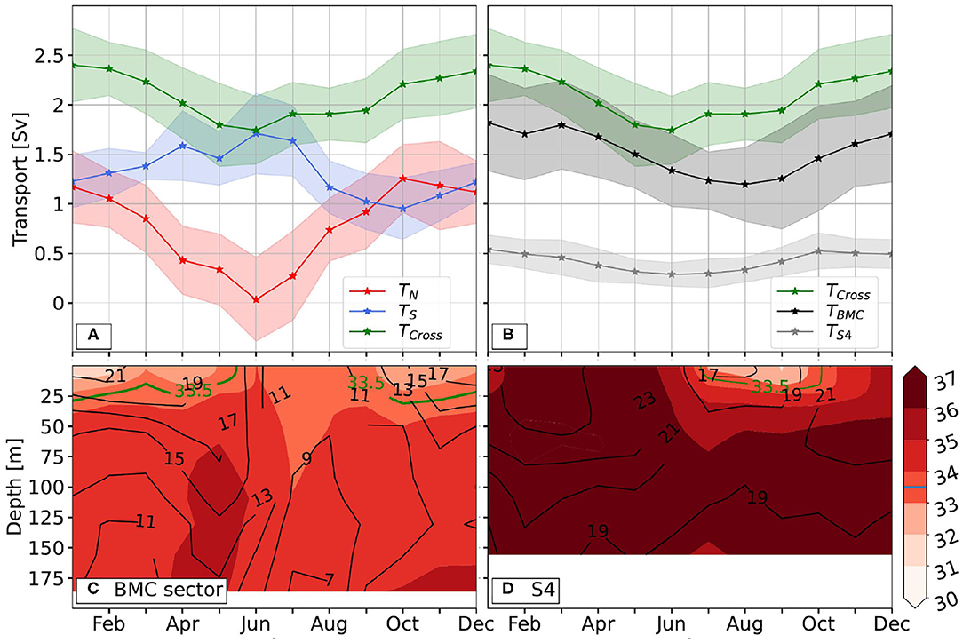
Figure 7. (A,B) Record length monthly mean transports (Sv, solid line) and standard deviation (shading), through 30°S (T_N, red), 40°S (T_S, blue), the shelf break between 30 and 40°S (T_Cross, green), the BMC (T_BMC, black), and S4 (T_S4, gray) segments. (C,D) Vertical distribution of the annual cycle of temperature (black contours, with 2°C contour interval) and salinity (background colors, with 1 contour interval, 33.5 shown by green line) averaged over the shelf break BMC (C) and S4 (D) sectors.

When analyzing the predominant export locations, the cross-shore transport through the BMC sector (T_BMC) presents subtly higher seasonal variability than T_Cross and similar spectral energy concentrated around one year (Supplementary Figure 2). The annual cycle of T_BMC (Figure 7B) shows a maximum (1.82 ± 0.49 Sv) in January and a minimum (1.20 ± 0.37 Sv) in August. The cross-shore transport through S4 (T_S4) also presents an annual cycle with a maximum (0.54 ± 0.18 Sv) in October and a minimum (0.28 ± 0.12 Sv) in June. At the seasonal scale, significant and positive correlations between T_Cross and T_BMC (0.55^*) and between T_Cross and T_S4 (0.77^*) are observed (Figure 8J). Most of the variability of T_S4 is associated with T_N (R² = 0.71^*, not shown). However, T_BMC presents no relationship with T_S (not shown). The seasonal component of T_S presents a negative correlation with T_S4 (R² = 0.30^*, not shown). However, it is difficult to identify a physical process that may explain this correlation.

FIGURE 8

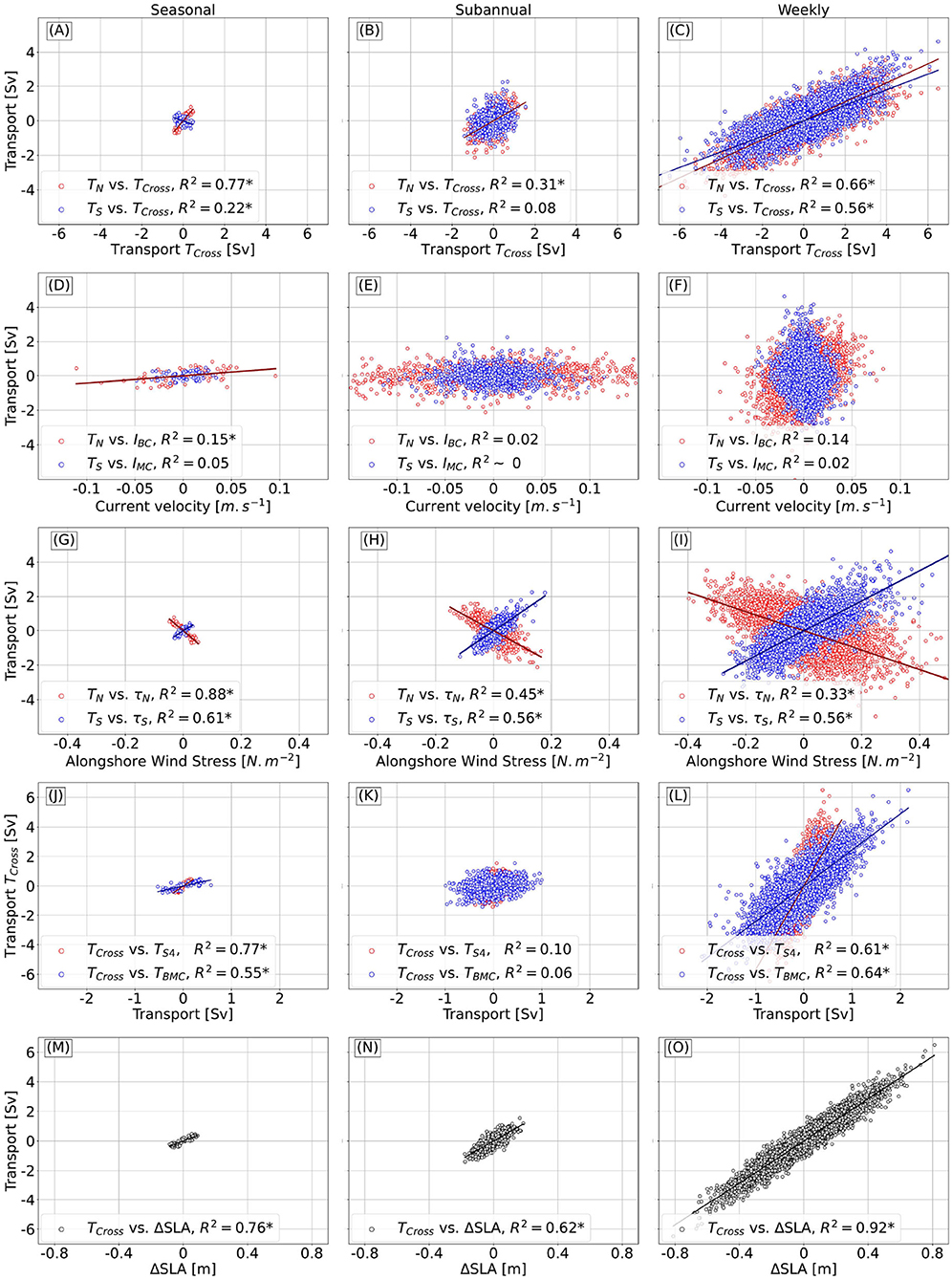
Figure 8. (A–C) T_N (red) and T_S (blue) vs. T_Cross. (D–F) T_N vs. I_BC (red) and T_S vs. I_MC (blue). (G–I) T_N vs. alongshore wind stress at 30°S (red) and T_S vs. alongshore wind stress at 40°S (blue). (J–L) T_Cross vs. T_S4 (red) and T_BMC (blue). (M–O) T_Cross vs. the difference of inner shelf SLA between 40 and 30°S. (A,D,G,J,M) Seasonal scale, (B,E,H,K,N) subannual scale and (C,F,I,L,O) weekly scale.

The climatology of the vertical temperature and salinity structure of the outer shelf averaged over the BMC sector is shown in Figure 7C. Note that on average the transport through this sector is offshore (positive) throughout the year (Figure 7B). Low salinity waters (S < 33.5), characteristic of shelf waters diluted by the RDP discharge, are present in the upper layer (z < 25 m) throughout the year, except in winter (JJA) when saltier and colder waters (S~33.8, < 11°C), associated with SASW are observed. Below this near-surface layer, waters with salinities between 33.8 and 35 are observed throughout the year. These waters represent mixtures of SASW with TW (Tropical Waters)/SACW. The salinity and temperature maxima observed during April–May and November are associated with a higher proportion of TW/SACW. On average the transport through S4 is also offshore (positive) throughout the year (Figure 7B). The vertical temperature and salinity structures are shown in Figure 7D. Low-salinities (S < 33.5) RDP waters are exported in the upper layer (z < 25 m) during July–October. During this period, at about 60 m depth, waters are warmer (>19°C) and saltier (>34) than in the upper layer. The rest of the year, saltier waters (S > 34) with surface temperatures ranging from 25.6 °C in March to 16.4 °C in July associated with STSW are exported to the open ocean through S4.

3.2.1.1. Drivers of Low Frequency (Interannual and Seasonal) Cross-Shore Transport Variability

In this section, we analyze the physical mechanisms driving offshore transport at low frequencies. At interannual scales, T_Cross is positively correlated with T_N and T_S, with R² = 0.40^* and 0.51^*, respectively (Supplementary Figure 3). Therefore, T_S has more control of T_Cross than T_N at this time scale in agreement with Combes and Matano (2018). The BMC location and T_Cross are not significantly correlated. To better understand the interannual variability of T_Cross, the T_S and T_N variability are further explored. To study the possible impact of the variability of the WBCs (Brazil and Malvinas currents), as suggested by numerical simulations (e.g., Matano et al., 2010), we compute the correlation between T_S and the intensity of the MC (I_MC) and between T_N and the intensity of the BC (I_BC). Another likely driver of T_Cross is the local alongshore wind defined as the wind stress vector at the boundary sections projected on the alongshore direction (38° from true North for both transects following the coastline). Local alongshore wind stress over the northern and southern sections was analyzed with southwesterly wind stress defined as positive. In the southern boundary, positive correlations at the interannual scale are observed between T_S and I_MC, with R² = 0.34^* (Supplementary Figure 3B) and T_S and alongshore wind stress with R² = 0.27 (not significant, Supplementary Figure 3C). At the northern boundary, T_N does not show a significant correlation with I_BC and alongshore wind stress.

At the seasonal scale, T_Cross variability presents a high positive correlation with T_N (R² = 0.77^*) and a negative correlation with T_S (R² = 0.22^*; Figure 8A). Thus, although the record-length mean T_Cross is mostly contributed by T_S, the variability at the seasonal scale is driven by variations in T_N. The BMC location and T_Cross are not correlated. These results are in agreement with Combes and Matano (2018). As the variability of the offshore transport is set by the variability of T_N and T_S, it is useful to further analyze the processes that determine the variations of the alongshore transports. The WBCs intensity was analyzed finding a low positive correlation between I_BC and T_N with R² 0.15^* and no correlation between I_MC and T_S (Figure 8D). T_N presents a strong and negative correlation with the alongshore wind stress (R² = 0.88^*, Figure 8G) in agreement with Combes et al. (2021). Therefore, high positive (southward) T_N is associated with northeasterly wind stress that sets up a negative SLA along the coast over the northern transect. The resulting cross-shore pressure gradient leads to a southwestward geostrophic flow through 30°S. Likewise, T_S presents a positive correlation with the alongshore wind stress (R² = 0.61^*, Figure 8G). Therefore, high T_S are associated with southwesterly wind stress that generates a positive SLA along the coast over the southern transect. The resulting cross-shore pressure gradient is related to a northeastward geostrophic flow through 40°S. The subtraction of the inner shelf SLA between the southern and northern boundaries represents 76% of the seasonal T_Cross variability (Figure 8M). In summary, the inner-shelf SLA variability at the boundaries (40 and 30°S) is a good indicator of the T_Cross variability at seasonal time scales.

3.2.2. High-Frequency Variability (Subannual and Weekly)

At the subannual scale, the variability of T_N, T_S, and T_Cross is larger than at low frequencies, with standard deviations of 0.82, 0.71, and 0.72 Sv, respectively (Table 2). The power spectra of transport variations show substantial energy (38.5, 40.4, and 22.5%, respectively) over a wide range of frequencies (Figure 6D). T_S4 and T_BMC are very weakly correlated with the transport variations at the northern and southern boundaries (R² < 0.15, Figure 8K).

At the weekly time scale, the standard deviations of T_N, T_S, and T_Cross increase to 0.90, 0.79, and 1.32 Sv, respectively (Table 2). The power spectra of the transport variability at the weekly time scale present high energy (47.0, 51.6, and 71.9%, respectively) over the entire frequency range (<10 days, Figure 6D). The transports through the preferential export routes are clearly related to the intensity of T_Cross with R² = 0.61^* and 0.64^* through the S4 and BMC sectors, respectively (Figure 8L). The T_S4 variability is more closely associated with the T_N variability (R² = 0.71^*, not shown) than to T_S (R² = 0.25^*, not shown), while the T_BMC variability is more closely associated with T_S variability (R² = 0.58^*, not shown) than to T_N (R² = 0.11, not shown).

3.2.2.1. Drivers of High-Frequency (Subannual and Weekly) Cross-Shore Transport Variability

Following the analysis of the low-frequency variability, the possible physical mechanisms modulating the high frequencies variability of T_Cross are analyzed. We investigate the possible relationship between the high-frequency variability of T_Cross and the location of the BMC, the shelf and WBCs transports, and the wind stress patterns. At the subannual scale, there is no significant correlation between T_Cross and T_S (Figure 8B) or with the location of the BMC (not shown). In contrast, T_Cross is primarily controlled by T_N (R² = 0.31^*, Figure 8B). T_N and T_S are driven by the local alongshore wind stress (R² = 0.45^* and 0.56^*, Figure 8H) and not by the WBCs (Figure 8E). As pointed out earlier, since local alongshore wind stress sets up SLA variations over the coast and similar to our findings at the seasonal time scale, the inner shelf SLA variations at the northern and southern boundaries are a good indicator of the T_Cross at subannual time scales. Changes in the inner shelf SLA difference at the southern and northern boundaries represent 62% of the T_Cross variability at subannual time scales (Figure 8N).

Numerical analyses indicate that although the location of the BMC does not modulate the magnitude of the export of shelf waters between 30 and 40°S, it does determine the position over the shelf break where the largest offshore transport occurs (Combes and Matano, 2018). Satellite and in-situ observations suggest that mesoscale eddies can induce the export of shelf waters (e.g., Guerrero et al., 2014; Manta et al., 2022). As these features have a typical time scale of 10–200 days, they could modulate the T_BMC at the subannual scale. The role of eddies in the cross-shore transports is further suggested by the significant decrease in correlation between the cross-shore (T_Cross) and the alongshore transports (T_N and T_S) at the subannual time scale (compare Figures 8A–C), and between T_Cross and the transport across the BMC sector (Figure 8K).

At the weekly time scale, there is no significant correlation between T_Cross and the BMC location (not shown). In contrast, T_Cross is closely associated with T_N and T_S (R² = 0.66^* and 0.56^*, respectively, Figure 8C). These alongshore transports are modulated by local alongshore wind stress over the northern and southern boundaries (R² = 0.33^* and 0.56^*, respectively, Figure 8I) and not by the intensity of WBCs (Figure 8F). These transport fluctuations are associated with the inner shelf SLA at 30 and 40°S. Similar to our findings at the seasonal and subannual time scales, the difference between inner shelf SLA at the southern and northern boundaries is a good proxy of T_Cross variability, representing 92% of the weekly variability (Figure 8O). These results are in agreement with Lago et al. (2021) who show that the alongshore transport can be estimated based on the difference in SLA between the coast and the shelf. Wind-forced coastal-trapped waves are an additional source of SLA variability at the weekly time scale (Brink, 1991; de Freitas et al., 2021). However, the details of the dynamics of processes leading to the model variability are deferred to a future study.

3.3. Analysis of Extreme Transport Events

In this section, the extreme cross-shore transport events are studied based on the daily, unfiltered T_N, T_S, and T_Cross. The monthly distribution of the number of positive extreme events is shown in Figure 9A. Recall positive transports imply northward flow over the shelf through 40°S (T_S), southward flow through 30°S (T_N), and offshore flow through the outer shelf between 30 and 40°S (T_Cross). Extreme southward (positive) T_N events (red bars in Figure 9A) occur more frequently in spring, last <3 days, and reach 6.32 Sv, eight-fold the mean value (0.78 Sv; Table 4). Extreme northward (positive) T_S events (blue bars in Figure 9A) are more frequent in austral winter (June–July) and infrequent in summer. Typically, the extreme transport events across the southern boundary last <4 days and reach transports of up to 8.36 Sv (Table 4), six-fold the mean value (1.31 Sv). The occurrence of positive T_Cross extreme events (green bars in Figure 9A) has two maxima, in fall and spring, and are less frequent in summer. The extreme export events have a shorter duration (<2 days) and present a maximum export transport of 9.45 Sv (more than four-fold the mean export transport, 2.09 Sv). During the entire period, the offshore transports across the BMC sector and S4 account for 73 and 20% of the total transport across the 200 m isobath between 30 and 40°S, respectively. However, during the extreme events, the transports across BMC and S4 decrease to 43 and 12% of the record-mean T_Cross. Therefore, the offshore transport during the extreme export events is spatially more uniformly distributed. During the average positive T_Cross export event (T_Cross mean of 6.08 Sv), 4.27% of the total volume of shelf waters between 30 and 40°S is exported to the open ocean.

FIGURE 9

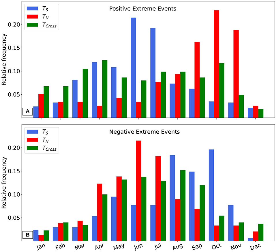
Figure 9. Histogram of monthly binned extreme transport events through 40°S (T_S, blue), 30°S (T_N, red), and cross-shore (T_Cross, green). (A) Positive extreme events. (B) Negative extreme events.

TABLE 4

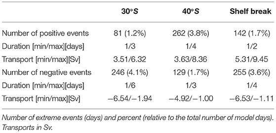
Table 4. Statistics of extreme transport events through selected sections.

The monthly distribution of the number of negative extreme events is shown in Figure 9B. Negative (northward) extreme T_N events are more frequent in June–July and uncommon in summer, last <6 days, and reach −6.54 Sv. Negative (southward) extreme T_S events occur more frequently between August and October and infrequently in summer, last <3 days, and reach transports of up to −4.92 Sv. The occurrence of negative extreme T_Cross events is maximum during winter and minimum during summer. The extreme cross-shore transport events have a short duration (between 1 and 4 days) and the maximum onshore transport reaches −6.53 Sv. During these negative cross-shore transport events the BMC sector continues to be an export location with offshore transports of shelf waters of 0.48 ± 0.64 Sv (Table 3). Therefore, the on-shelf intrusion of open ocean water is distributed over the remaining of the shelf break domain (Figure 5B), including S4. These negative extreme events represent on average 1.79% of the total shelf volume between 30 and 40°S.

The extreme events have a typical duration in the weekly time scale. As discussed in section 3.2.2.1, the variability on this scale is mostly driven by the local alongshore wind stress. Therefore, it is useful to further explore the possible association between variations in regional wind patterns and extreme transport events. Recall that southwesterly wind stress is referred to as positive and northeasterly wind stress as negative. A composite (average fields during extreme events) of positive T_N extreme events is characterized by negative (northeasterly) local alongshore wind stress (~−0.27 N.m⁻²) at 30°S associated with a high atmospheric pressure center located near 40°S–35°W (Figure 10A). Consequently, a negative SLA develops along the coast, which is most intense north of the RDP estuary. The resulting cross-shore pressure gradient leads to a southwestward geostrophic flow north of 38°S. The negative SLA and the associated geostrophic flow weaken near the southern boundary. The negative T_N extreme events are characterized by positive local alongshore wind stress (~0.16 N.m⁻²) at 30°S, associated with a high atmosphere pressure center located near 32.5°S–59.5°W (Figure 10D). Consequently, a positive SLA develops along the coast north of 38°S, which leads to a northeastward geostrophic flow at 30°S.

FIGURE 10

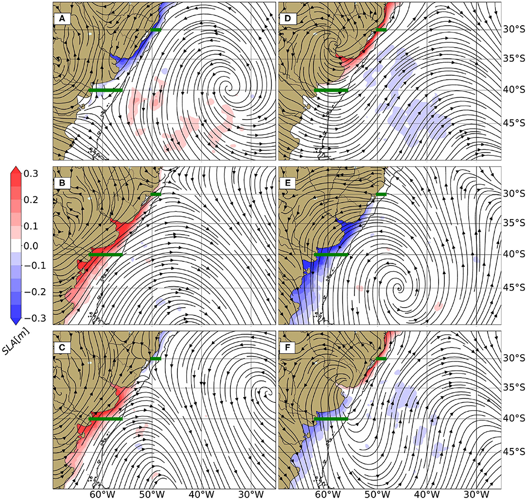
Figure 10. Composite of model derived sea level anomaly (background color shading) and black streamlines show surface wind patterns during positive (A) and negative (D) extreme T_N events. (B) and (E), same as (A,D) for T_S. (C) and (F), same as (A,D) for T_Cross. The 200 m isobath is indicated by a gray line.

The positive extreme events in T_S are associated with positive (southwesterly) local alongshore wind stress (~0.21 N.m⁻²) at 40°S, associated with a low atmospheric pressure center located south of 50°S (Figure 10B), that generates southwesterly wind stress over the continental shelf south of 30°S. This intense wind stress creates a positive SLA along the coast in the entire domain, which leads to a relatively strong northeastward geostrophic flow at 40°S. This northeastward flow extends northeastward, also leading to northeastward (negative) flow across the northern boundary. Conversely, negative T_S extreme events are associated with negative (northeasterly) local alongshore wind stress at 40°S (~−0.13 N.m⁻²) associated with a high atmospheric pressure center located at 45°S–47.5°W (Figure 10E). In response to this wind stress pattern, there is a negative inner shelf SLA south of 30°S and an associated southwestward flow across the southern boundary (Figure 10E).

The positive T_Cross extreme events are characterized by southwesterly wind stress at 40°S (~0.22 N.m⁻²) and northeasterly wind stress at 30°S (~−0.08 N.m⁻²). A low atmospheric pressure center located near 50°S–50°W (Figure 10C) generates southwesterly wind stress over the continental shelf south of 40°S and a positive SLA along the coast south of 34°. Thus, this atmospheric circulation pattern leads to relatively intense northeastward transport (4.03 ± 1.69 Sv, Table 3) over the shelf across the southern boundary (T_S, 40°S). Conversely, a high atmospheric pressure center located near 35°S–28°W generates northeasterly wind stress over the continental shelf north of 30°S. In response to this wind stress pattern, a weak negative SLA develops in the inner shelf north of 33°S, this negative anomaly leads to southwestward transport (2.02 ± 1.57 Sv, Table 3) over the shelf across the northern boundary (T_N, 30°S). The resulting mass convergence over the shelf between 30 and 40°S is compensated by a strong offshore flow of shelf waters. The negative extreme events of T_Cross are associated with a high atmospheric pressure center located over the RDP (Figure 10F). This feature leads to northwesterly wind stress at 40°S (~−0.04 N.m⁻²) that generates a negative SLA over the coast south of the RDP and southwesterly wind stress at 30°S (~0.14 N.m⁻²) that generates a positive SLA north of RDP. As a result, a weakening of northeastward flow across the southern boundary (T_S, 0.14 ± 1.28 Sv) and a northeastward transport across the northern boundary are observed (T_N, −2.16 ± 1.42 Sv). Analogous to the positive extreme events, the mass divergence over the shelf between 30 and 40°S is compensated by an influx of deep-ocean waters to the shelf. These import events can have an important biogeochemical impact on the shelf.

Intense Malvinas Current intrusions over the shelf, causing substantial cooling, increased salinity, and elevated surface chlorophyll concentrations have been reported near 41°S (Piola et al., 2010). A recent analysis of in-situ observations collected in late April 2016 between 34 and 38°S presents relatively cold, salty, and high-nutrient waters in the outer shelf near 36.5°S (Manta et al., 2022, their Figures 2C,F, 5C). These observations suggest onshore flow of subantarctic water from the Malvinas Current. Our model analysis indicates that T_Cross reached −2.55 Sv in the previous days. About 30% of this inflow occurred across the BMC (T_BMC ~−0.81 Sv). As might be expected, on average T_BMC is positive and peaks in the BMC sector of the shelf-break (Supplementary Figure 4). However, there are a few instances (about 2.20% of the time) when T_BMC is negative (onshore), as observed in late April 2016. In the model, the relatively intense import of slope waters was associated with northeastward flows of −4.09 Sv across 30°S and 1.54 Sv across 40°S, which peaked on 27 April 2016. Thus, the model circulation is consistent with the observation of subantarctic waters in the outer shelf south of the BMC reported by Manta et al. (2022). Moreover, the model results suggest that the onshelf flow observed in late April 2016 between 30 and 40° was a response to divergence of the along-shore circulation, which was mostly driven by the pattern of alongshore winds. However, in agreement with the observations of Manta et al. (2022), mesoscale eddies that approach the outer shelf may create a fine scale structure of relatively intense cross-shore flows (see Supplementary Figure 5). In addition, highly non-linear submesoscale features of characteristic scale <10 km, not resolved by the GLORYS reanalysis, are ubiquitous in the Brazil/Malvinas Confluence (Orúe-Echevarŕıa et al., 2019), and may further contribute to cross-shelf exchanges.

3.3.1. The T_Cross Event of Early May 2015

From 29 April to 3 May 2015 the model produces large transport anomalies across 40°S. This event is of interest because it was also clearly detected by direct current observations close to 40°S (see section 3.1.3 and Lago et al., 2019, 2021). On 29 April 2015, the circulation is characteristic of an extreme negative T_S event, with northeasterly wind stress (Figure 11A) generating a negative inner shelf SLA associated with southwestward flow over the shelf south of 33°S (Figure 11C). At that time the flow over much of the shelf is southward, reaching −1.82 Sv across 40°S and +0.8 Sv across 30°S. Recall that we have defined southward flow at 30°S as positive. In response to the divergence of the alongshore circulation, T_Cross presents a negative (onshore) transport (−1.03 Sv) (Table 3). The flow structure indicates intrusions of slope waters: relatively cold-salty waters from the MC south of 37°S and warm-salty waters from the BC near 31°S (Figure 11B). On 3 May, the circulation has evolved to one that is characteristic of extreme offshore transport events with T_Cross reaching 8.80 Sv (Table 3). This very large export of relatively fresh shelf waters (Figure 11E) is mediated by strong convergence of the alongshore circulation over the shelf (Figure 11F). At that time the flow across 40°S reverses to northward, with T_S reaching 5.36 Sv in response to a positive SLA over the inner shelf generated by local southwesterly/westerly wind stress (Figure 11D). In contrast, the flow at 30°S is still southwestward (positive), with T_N reaching 3.44 Sv, in response to a negative SLA over the inner shelf which in turn results from local northeasterly wind stress at that location. Shelf water export during extreme events does not necessarily follow the most frequently observed pathways across the BMC and S4 segments, it occurs across most of the shelf break, with a maximum export occurring between 32 and 36.5°S.

FIGURE 11

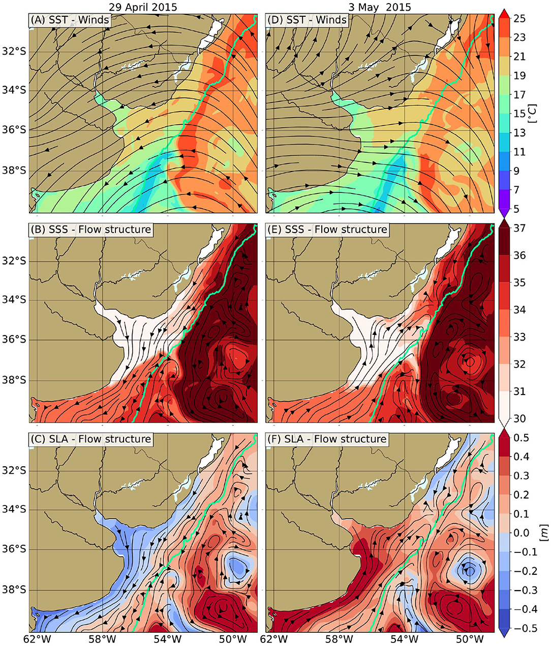
Figure 11. SST (°C, A,D), SSS (B,E), SLA (m, C,F) are shown in colors (color scale at right). Black streamlines show the flow structure over the upper 200 m (B,C,E,F) and surface wind patterns from ERA5 (A,D). The left panels (A–C) present the fields on 29 April 2015 and the right panels (D–F) on 3 May 2015. The 200 m isobath is indicated by a green line.

4. Summary and Conclusions

The variability and drivers of the cross-shelf exchanges between the Southwestern Atlantic shelf between 30 and 40°S and the open ocean have been analyzed using a high-resolution ocean reanalysis. Independent hydrographic data from 12 oceanographic surveys carried out on the shelf near 34°S between 2003 and 2018, 24 years of gridded altimetry data (note that GLORYS12V1 assimilates along-track altimetry), and an independent estimate of alongshore transport near 39°S based on mooring data were used to evaluate the model performance. There is a substantial agreement near 39°S between daily alongshore shelf transports from observations and the model. The model also shows similar patterns of SLA variability to the altimetry derived data, although with somewhat larger differences over the Río de la Plata. The relatively low spatial and temporal resolution of the gridded altimetric product does not allow the representation of mesoscale, high-frequency processes (3–10 day periods) which are generated by the model's internal dynamics. In addition, the model presents an overall good agreement with geostrophic velocities calculated from the hydrographic data over the shelf near 34°S.

Once the reanalysis performance was assessed, we analyzed the cross-shore transport and its temporal and spatial variability. The record length mean cross-shore transport [mean ± standard deviation] between 30 and 40°S (T_Cross) is 2.09 ± 1.60 Sv, with positive transport representing offshore flow. Sixty-three percent of the mean T_Cross was contributed by northward transport across 40°S (T_S) and the remaining 37% by southward transport across 30°S (T_N). Most of the offshore flow (73%) occurs in the vicinity of the BMC and about 20% in the vicinity of 32°S. T_Cross presents more variability at high frequencies, 71.9 and 22.5% of energy in the weekly and subannual scales, respectively than at low frequencies, 4.9 and 0.7% of energy in the seasonal and interannual scales, respectively.

At the interannual scale, the cross-shore transport variability (T_Cross) is more controlled by the alongshore transport over the shelf across 40°S (T_S, 51%) than across 30°S (T_N, 40%) and T_S is moderately modulated by the intensity of the Malvinas Current. At the annual scale, there is high spectral energy in all transports. In the mean, T_N and T_S are positive throughout the year. T_N presents a maximum (southwestward) transport in October and a minimum from April to July while T_S has the opposite behavior, though with somewhat weaker amplitude. Consequently, T_Cross is positive (offshore) throughout the year, and presents a maximum in January and a minimum in June. The alongshore transports over the shelf are driven by local alongshore wind stress. T_Cross variability is mostly driven by T_N variability. At the subannual scale, T_N and T_S are driven by the local alongshore wind stress and T_Cross, particularly near 32°S, is primarily controlled by T_N. At the weekly time scale, both T_N and T_S are also strongly modulated by the local alongshore wind stress. T_S has control over the export of shelf waters across the BMC, while T_N is more closely associated with cross-shore fluxes at 32°S.

Extreme alongshore transport events across 30 and 40°S have been analyzed using the model's daily output. These events are closely associated with local wind stress with a duration of <6 and 4 days, respectively. During positive events, defined as convergence of alongshore flow over the shelf, transports reach 6 and 8 times their long-term averages, respectively. Extreme offshore transport events reach up to 9.45 Sv. These high export events last <2 days and are more frequent during fall and spring. Despite the short duration of intense export events, 4.3% of the total volume of shelf water between 30 and 40°S is exported to the adjacent deep ocean during the average event (6.05 Sv). These large exports of shelf waters must lead to freshening of upper ocean waters as revealed by in-situ and satellite observations. In contrast, negative extreme events drive open ocean water intrusions of up to 6.53 Sv. These onshore flow events last <4 days and are more frequent in winter. During the average onshore flow event, 1.8% of the total volume of shelf water is replaced by slope water. The inflows of open ocean waters, particularly those of salty subtropical waters from the Brazil Current, must cause a substantial salinification of outer shelf waters and those from the Malvinas Currents contribute with nutrients.

Alongshore winds over the shelf generate SLAs over the inner shelf. The associated cross-shore pressure gradient leads to alongshore geostrophic flows. Southwesterly winds over the southern boundary (40°S) drive a positive SLA on the inner shelf and northeasterly winds over the northern boundary (30°S) generate a negative SLA on the inner shelf. The resulting cross-shore pressure gradients drive convergent alongshore geostrophic flows over the shelf and export of shelf waters to the open ocean. Conversely, opposite winds generate divergent alongshore geostrophic flows over the shelf and drive the import of slope water to the shelf. These SLA variations on the inner shelf, mostly controlled by alongshore wind variations, exert an important control on alongshore circulation, and cross-shelf exchange, on seasonal, subannual, and weekly scales and also on the extreme events.

Data Availability Statement

Publicly available datasets were analyzed in this study. These data can be found at: GLORYS12V1 ocean reanalysis (https://resources.marine.copernicus.eu/documents/QUID/CMEMS-GLO-QUID-001-030.pdf); ERA5 atmospheric reanalysis (https://www.ecmwf.int/en/forecasts/datasets/reanalysis-datasets/era5); and altimetry data from Copernicus Marine https://resources.marine.copernicus.eu/product-detail/SEALEVEL_GLO_PHY_L4_MY_008_047/INFORMATION). In situ data located near 39° used to evaluate the model performance can be found in public SE-ANOE public data repository at: https://www.seanoe.org/data/00403/51492/ and https://www.seanoe.org/recordview. Hydrographic data near 34° used to evaluate the model performance can be found in public data repository at ftp://ftp.aoml.noaa.gov/phod/pub/SAM/hydrographic_data/, in this in-text data citation references: Charo et al. (2020).

Author Contributions

GB processed the hydrographic and the model data and did the model performance evaluation and the transport calculations and prepared the manuscript with contributions from all co-authors. All authors participated in the scientific interpretation of the results. All authors contributed to the article and approved the submitted version.

Funding

This work was partially funded by the Inter-American Institute for Global Change Research (IAI) grants CRN3070 (US National Science Foundation grant GEO-1128040) and SGP-HW 017. Additional funding was provided by IAI/CONICET grant RD3347, FONCYT grant PICT2016-0557, and SECYT-UNS grant 24-F079.

Conflict of Interest

The authors declare that the research was conducted in the absence of any commercial or financial relationships that could be construed as a potential conflict of interest.

Publisher's Note

All claims expressed in this article are solely those of the authors and do not necessarily represent those of their affiliated organizations, or those of the publisher, the editors and the reviewers. Any product that may be evaluated in this article, or claim that may be made by its manufacturer, is not guaranteed or endorsed by the publisher.

Acknowledgments

GB was supported by a doctoral fellowship from Consejo Nacional de Investigaciones Científicas y Técnicas (Argentina). The hydrographic data were collected as part of the South Atlantic Meridional Overturning Circulation initiative (https://www.aoml.noaa.gov/phod/SAMOC_international/). We thank the science parties and crews of the NICOP/Plata, SAM, and STSF cruises that collected the data in the Albardão transect. We particularly thank Marcela Charo (SHN, Argentina) for data calibration and processing and Loreley Lago (CIMA, Argentina) for providing the observational transport time series shown in Figure 4.

Supplementary Material

The Supplementary Material for this article can be found online at: https://www.frontiersin.org/articles/10.3389/fmars.2022.855183/full#supplementary-material

References

Ballarotta, M., Ubelmann, C., Pujol, M.-I., Taburet, G., Fournier, F., Legeais, J.-F., et al. (2019). On the resolutions of ocean altimetry maps. Ocean Sci. 15, 1091–1109. doi: 10.5194/os-15-1091-2019

CrossRef Full Text | Google Scholar

Berden, G., Charo, M., Möller, O. O. Jr, and Piola, A. R. (2020). Circulation and hydrography in the western south Atlantic shelf and export to the deep adjacent ocean: 30°S to 40°S. J. Geophys. Res. 125, e2020JC016500. doi: 10.1029/2020JC016500

CrossRef Full Text | Google Scholar

Bordin, L. H., Machado, E. d. C., Carvalho, M., Freire, A. S., and Fonseca, A. L. (2019). Nutrient and carbon dynamics under the water mass seasonality on the continental shelf at the South Brazil Bight. J. Mar. Syst. 189, 22–35. doi: 10.1016/j.jmarsys.2018.09.006

CrossRef Full Text | Google Scholar

Borús, J., Uriburu Quirno, M., and Calvo, D. (2017). Evaluación de Caudales Mensuales Descargados por los Grandes ríos del Sistema del Plata al Estuario del Río de la Plata. Ezeiza: Alerta Hidrológico-Instituto Nacional del Agua y el Ambiente.

Google Scholar

Braga, E. S., Chiozzini, V. C., Berbel, G. B., Maluf, J. C., Aguiar, V. M., Charo, M., et al. (2008). Nutrient distributions over the Southwestern South Atlantic continental shelf from Mar del Plata (Argentina) to Itajaí(Brazil): winter-summer aspects. Contin. Shelf Res. 28, 1649–1661. doi: 10.1016/j.csr.2007.06.018

CrossRef Full Text | Google Scholar

Brink, K.. (1991). Coastal-trapped waves and wind-driven currents over the continental shelf. Annu. Rev. Fluid Mech. 23, 389–412. doi: 10.1146/annurev.fl.23.010191.002133

CrossRef Full Text | Google Scholar

Cabanes, C., Grouazel, A., von Schuckmann, K., Hamon, M., Turpin, V., Coatanoan, C., et al. (2013). The CORA dataset: validation and diagnostics of in-situ ocean temperature and salinity measurements. Ocean Sci. 9, 1–18. doi: 10.5194/os-9-1-2013

CrossRef Full Text | Google Scholar

Charo, M., Guerrero, R., and Piola, A. (2020). Subtropical Shelf Front cruise-Conductivity-Temperature-Depth (CTD) Data. Harvard Dataverse.

Google Scholar

Chen, C.-T. A., Liu, K.-K., and Macdonald, R. (2003). “Continental margin exchanges,” in Ocean Biogeochemistry, Fasham MJR, editor (Berlin: Springer), 53–97. doi: 10.1007/978-3-642-55844-3_4

PubMed Abstract | CrossRef Full Text | Google Scholar

Chidichimo, M., Piola, A., Meinen, C., Perez, R., Campos, E., Dong, S., et al. (2021). Brazil current volume transport variability during 2009-2015 from a long-term moored array at 34.5°S. J. Geophys. Res. 126, e2020JC017146. doi: 10.1029/2020JC017146

CrossRef Full Text | Google Scholar

Christensen, J. P., Murray, J. W., Devol, A. H., and Codispoti, L. A. (1987). Denitrification in continental shelf sediments has major impact on the oceanic nitrogen budget. Glob. Biogeochem. Cycles 1, 97–116. doi: 10.1029/GB001i002p00097

CrossRef Full Text | Google Scholar

Ciotti, Á. M., Odebrecht, C., Fillmann, G., and Moller, O. O. Jr (1995). Freshwater outflow and Subtropical Convergence influence on phytoplankton biomass on the southern Brazilian continental shelf. Cont. Shelf Res. 15, 1737–1756. doi: 10.1016/0278-4343(94)00091-Z

CrossRef Full Text | Google Scholar

Combes, V., and Matano, R. P. (2014a). Trends in the Brazil/Malvinas confluence region. Geophys. Res. Lett. 41, 8971–8977. doi: 10.1002/2014GL062523

CrossRef Full Text | Google Scholar

Combes, V., and Matano, R. P. (2014b). A two-way nested simulation of the oceanic circulation in the southwestern Atlantic. J. Geophys. Res. 119, 731–756. doi: 10.1002/2013JC009498

CrossRef Full Text | Google Scholar

Combes, V., and Matano, R. P. (2018). The Patagonian shelf circulation: drivers and variability. Prog. Oceanogr. 167, 24–43. doi: 10.1016/j.pocean.2018.07.003

CrossRef Full Text | Google Scholar

Combes, V., Matano, R. P., and Palma, E. D. (2021). Circulation and cross-shelf exchanges in the northern shelf region of the southwestern Atlantic: kinematics. J. Geophys. Res. 126, e2020JC016959. doi: 10.1029/2020JC016959

CrossRef Full Text | Google Scholar

de Freitas, P. P., de Moraes Paiva, A., Cirano, M., Mill, G. N., da Costa, V. S., Gabioux, M., et al. (2021). Coastal trapped waves propagation along the southwestern Atlantic continental shelf. Cont. Shelf Res. 226, 104496. doi: 10.1016/j.csr.2021.104496

CrossRef Full Text | Google Scholar

de Haas, H., van Weering, T. C., and de Stigter, H. (2002). Organic carbon in shelf seas: sinks or sources, processes and products. Cont. Shelf Res. 22, 691–717. doi: 10.1016/S0278-4343(01)00093-0

CrossRef Full Text | Google Scholar

Franco, B. C., Palma, E. D., Combes, V., Acha, E. M., and Saraceno, M. (2018). Modeling the offshore export of Subantarctic Shelf Waters from the Patagonian shelf. J. Geophys. Res. 123, 4491–4502. doi: 10.1029/2018JC013824

CrossRef Full Text | Google Scholar

Franco, B. C., Palma, E. D., Combes, V., and Lasta, M. L. (2017). Physical processes controlling passive larval transport at the Patagonian Shelf Break Front. J. Sea Res. 124, 17–25. doi: 10.1016/j.seares.2017.04.012

CrossRef Full Text | Google Scholar

Gattuso, J.-P., Frankignoulle, M., and Wollast, R. (1998). Carbon and carbonate metabolism in coastal aquatic ecosystems. Annu. Rev. Ecol. Syst. 29, 405–434. doi: 10.1146/annurev.ecolsys.29.1.405

CrossRef Full Text | Google Scholar

Goni, G. J., and Wainer, I. (2001). Investigation of the Brazil Current front variability from altimeter data. J. Geophys. Res. 106, 31117–31128. doi: 10.1029/2000JC000396

CrossRef Full Text | Google Scholar

Gordon, A. L., and Greengrove, C. L. (1986). Geostrophic circulation of the Brazil-Falkland confluence. Deep Sea Res. Part A.Oceanogr. 33, 573–585. doi: 10.1016/0198-0149(86)90054-3

CrossRef Full Text | Google Scholar

Guerrero, R. A., Piola, A. R., Fenco, H., Matano, R. P., Combes, V., Chao, Y., et al. (2014). The salinity signature of the cross-shelf exchanges in the Southwestern Atlantic Ocean: satellite observations. J. Geophys. Res. 119, 7794–7810. doi: 10.1002/2014JC010113

PubMed Abstract | CrossRef Full Text | Google Scholar

Hersbach, H., Bell, B., Berrisford, P., Hirahara, S., Horányi, A., Mu noz-Sabater, J., et al. (2020). The era5 global reanalysis. Q. J. R. Meteorol. Soc. 146, 1999–2049. doi: 10.1002/qj.3803

CrossRef Full Text | Google Scholar

Hirschi, J. J., Killworth, P. D., and Blundell, J. R. (2007). Subannual, seasonal, and interannual variability of the North Atlantic meridional overturning circulation. J. Phys. Oceanogr. 37, 1246–1265. doi: 10.1175/JPO3049.1

CrossRef Full Text | Google Scholar

Lago, L. S., Saraceno, M., Martos, P., Guerrero, R. A., Piola, A. R., Paniagua, G. F., et al. (2019). On the wind contribution to the variability of ocean currents over wide continental shelves: a case study on the northern Argentine continental shelf. J. Geophys. Res. 124, 7457–7472. doi: 10.1029/2019JC015105

CrossRef Full Text | Google Scholar

Lago, L. S., Saraceno, M., Piola, A. R., and Ruiz-Etcheverry, L. A. (2021). Volume transport variability on the northern argentine continental shelf from in situ and satellite altimetry data. J. Geophys. Res. 126, e2020JC016813. doi: 10.1029/2020JC016813

CrossRef Full Text | Google Scholar

Lellouche, J.-M., Greiner, E., Le Galloudec, O., Garric, G., Regnier, C., Drevillon, M., et al. (2018). Recent updates to the Copernicus Marine Service global ocean monitoring and forecasting real-time 1/12° high-resolution system. Ocean Sci. 14, 1093–1126. doi: 10.5194/os-14-1093-2018

CrossRef Full Text | Google Scholar

Lumpkin, R., and Garzoli, S. (2011). Interannual to decadal changes in the western South Atlantic's surface circulation. J. Geophys. Res. 116, 1–10. doi: 10.1029/2010JC006285

CrossRef Full Text | Google Scholar

Madec, G., Bourdallé-Badie, R., Bouttier, P.-A., Bricaud, C., Bruciaferri, D., Calvert, D., et al. (2017). Nemo Ocean Engine. Note du Pôle de Modélisation de l'Institut Pierre-Simon Laplace, No. 27. Institut Pierre-Simon Laplace.

Google Scholar

Malan, N., Archer, M., Roughan, M., Cetina-Heredia, P., Hemming, M., Rocha, C., et al. (2020). Eddy-driven cross-shelf transport in the East Australian Current separation zone. J. Geophys. Res. 125, e2019JC015613. doi: 10.1029/2019JC015613

CrossRef Full Text | Google Scholar

Manta, G., Speich, S., Barreiro, M., Trinchin, R., De Mello, C., Laxenaire, R., et al. (2022). Shelf water export at the brazil-malvinas confluence evidenced from combined in-situ and satellite observations. Front. Marine Sci. doi: 10.3389/fmars.2022.857594. [In Press].

CrossRef Full Text | Google Scholar

Matano, R., Palma, E. D., and Piola, A. R. (2010). The influence of the Brazil and Malvinas Currents on the Southwestern Atlantic Shelf circulation. Ocean Sci. 6, 983–995. doi: 10.5194/os-6-983-2010

CrossRef Full Text | Google Scholar

Matano, R. P., Combes, V., Piola, A. R., Guerrero, R., Palma, E. D., Ted Strub, P., et al. (2014). The salinity signature of the cross-shelf exchanges in the Southwestern Atlantic Ocean: numerical simulations. J. Geophys. Res. 119, 7949–7968. doi: 10.1002/2014JC010116

PubMed Abstract | CrossRef Full Text | Google Scholar

Möller, O. O. Jr, Piola, A. R., Freitas, A. C., and Campos, E. J. (2008). The effects of river discharge and seasonal winds on the shelf off southeastern South America. Cont. Shelf Res. 28, 1607–1624. doi: 10.1016/j.csr.2008.03.012

CrossRef Full Text | Google Scholar

Orúe-Echevarría, D., Castellanos, P., Sans, J., Emelianov, M., Vallés-Casanova, I., and Pelegrí, J. L. (2019). Temperature spatiotemporal correlation scales in the Brazil-Malvinas Confluence from high-resolution in situ and remote sensing data. Geophys. Res. Lett. 46, 13234–13243. doi: 10.1029/2019GL084246

CrossRef Full Text | Google Scholar

Palma, E., Matano, R., and Piola, A. (2004). A numerical study of the Southwestern Atlantic Shelf circulation: Barotropic response to tidal and wind forcing. J. Geophys. Res. 109, C08014. doi: 10.1029/2004JC002315

CrossRef Full Text | Google Scholar

Palma, E. D., and Matano, R. P. (2009). Disentangling the upwelling mechanisms of the south Brazil bight. Cont. Shelf Res. 29, 1525–1534. doi: 10.1016/j.csr.2009.04.002

CrossRef Full Text | Google Scholar

Piola, A. R., Campos, E. J., Möller, O. O. Jr, Charo, M., and Martinez, C. (2000). Subtropical shelf front off eastern South America. J. Geophys. Res. 105, 6565–6578. doi: 10.1029/1999JC000300

CrossRef Full Text | Google Scholar

Piola, A. R., Martínez Avellaneda, N., Guerrero, R. A., Jardon, F. P., Palma, E. D., and Romero, S. I. (2010). Malvinas-slope water intrusions on the northern Patagonia continental shelf. Ocean Sci. 6, 345–359. doi: 10.5194/os-6-345-2010

CrossRef Full Text | Google Scholar

Piola, A. R., Matano, R. P., Palma, E. D., Moller, O. O., and Campos, E. J. D. (2005). The influence of the Plata River discharge on the western South Atlantic shelf. Geophys. Res. Lett. 32, 1–4. doi: 10.1029/2004GL021638

CrossRef Full Text | Google Scholar

Piola, A. R., Möller, O. O. Jr, Guerrero, R. A., and Campos, E. J. (2008). Variability of the subtropical shelf front off eastern South America: Winter 2003 and summer 2004. Cont. Shelf Res. 28, 1639–1648. doi: 10.1016/j.csr.2008.03.013

CrossRef Full Text | Google Scholar

Piola, A. R., Palma, E. D., Bianchi, A. A., Castro, B. M., Dottori, M., Guerrero, R. A., et al. (2018). “Physical oceanography of the SW Atlantic Shelf: a review,” in Plankton Ecology of the Southwestern Atlantic–From the Subtropical to the Subantarctic Realm, eds M. Hoffmeyer, M. E. Sabatini, F. Brandini, D. Calliari, and N. Santinelli (Cham: Springer), 37–56. doi: 10.1007/978-3-319-77869-3_2

CrossRef Full Text | Google Scholar

Pujol, M.-I., Faugére, Y., Taburet, G., Dupuy, S., Pelloquin, C., Ablain, M., et al. (2016). Duacs DT2014: the new multi-mission altimeter data set reprocessed over 20 years. Ocean Sci. 12, 1067–1090. doi: 10.5194/os-12-1067-2016

CrossRef Full Text | Google Scholar

Rabouille, C., Mackenzie, F. T., and Ver, L. M. (2001). Influence of the human perturbation on carbon, nitrogen, and oxygen biogeochemical cycles in the global coastal ocean. Geochim. Cosmochim. Acta 65, 3615–3641. doi: 10.1016/S0016-7037(01)00760-8

CrossRef Full Text | Google Scholar

Reynolds, R. W., Smith, T. M., Liu, C., Chelton, D. B., Casey, K. S., and Schlax, M. G. (2007). Daily high-resolution-blended analyses for sea surface temperature. J. Clim. 20, 5473–5496. doi: 10.1175/2007JCLI1824.1

PubMed Abstract | CrossRef Full Text | Google Scholar

Roughan, M., Macdonald, H. S., Baird, M. E., and Glasby, T. M. (2011). Modelling coastal connectivity in a Western Boundary Current: Seasonal and inter-annual variability. Deep Sea Res. Part II Top. Stud. Oceanogr. 58, 628–644. doi: 10.1016/j.dsr2.2010.06.004

CrossRef Full Text | Google Scholar

Strub, P. T., James, C., Combes, V., Matano, R. P., Piola, A. R., Palma, E. D., et al. (2015). Altimeter-derived seasonal circulation on the Southwest Atlantic shelf: 27°−43°S. J. Geophys. Res. 120, 3391–3418. doi: 10.1002/2015JC010769

PubMed Abstract | CrossRef Full Text | Google Scholar