Design of an Optimal Testbed for Acoustic Tags: Test Case for Marine Megafauna

Underwater acoustic technologies are a key component for exploring the behavior of marine fauna such as sea turtles, sharks, and seals. The animals are marked with acoustic devices (tags) that periodically emit signals encoding the device’s ID along with sensor data such as depth, temperature, or the dominant acceleration axis - data that is collected by a network of deployed receivers. In this work, we aim to optimize the locations of receivers for best tracking of acoustically tagged marine fauna, and provide a test case with tags suitable for megafauna tracking. The outcomes of such tracking allows the evaluation of the animals’ motion patterns, their hours of activity, and their social interactions. In particular, we focus on how to determine the receivers’ deployment positions to maximize the coverage area in which the tagged animals can be tracked. For example, an overly-condensed deployment may not allow accurate tracking, whereas a sparse one, may lead to a small coverage area due to too few detections. We formalize the question of where to best deploy the receivers as a non-convex constraint optimization problem that takes into account the local environment and the specifications of the tags, and offer a sub-optimal, low-complexity solution that can be applied to large testbeds. Numerical investigation for three stimulated sea environments shows that our proposed method is able to increase the localization coverage area by 30%, and results from a test case experiment demonstrate similar performance in a real sea environment. We share the implementation of our work to help researchers set up their own acoustic observatory.

Introduction

Underwater acoustic tracking is a key enabling technology for exploring long-term behavior of marine fauna (Kraus et al., 2018). Acoustic telemetry of fish developed in the mid 1950s by the U.S. Bureau of Commercial Fisheries (BCF), enabling the identification and localization of the individual fish without the need to recapture it (Hockersmith and Beeman, 2012). Tracking of decapod crustaceans with acoustic telemetry devices evolved since the 1970s and as of toady 60% of published studies are based on acoustic telemetry (Florko et al., 2021), mostly using acoustic tags. Although tracking of fauna can be performed by passive and active system, e.g., (Diamant et al., 2019), the data obtained from acoustic tagging is far more informative. As a result, acoustic tagging is used in multitude of research projects such as the ocean tracking network (OTN) (https://oceantrackingnetwork.org/). For marine megafauna, acoustic tags have been used for understanding the behavioral and social interactions of animals like sharks, sea turtles, and seals (Berejikian et al., 2016; Lea et al., 2016). Anchored receivers are deployed in known locations within the explored area to decode and measure the time of arrival (ToA) of the tags’ emissions for, usually offline, tracking of the tagged animals. The long-term durability of the tags and receivers that can operate for many months and years allows operation over a long period of time for the statistical evaluation of the activity of the tagged animals. Examples of tagged sharks (Lea et al., 2016) and turtles (Thums et al., 2013) revealed valuable information about the animals’ local motion patterns, their hours of activity, and their social interactions.

The detection of the animal’s tag emissions using a single receiver is sufficient for collecting indications of presence/absence of an animal in an area of interest (Jackson, 2011; Gazit et al., 2013). However, in the case of fixed receivers, receptions of a tag’s emissions by at least three receivers is required to localize the animal in a two-dimensional (2D) plane with no ambiguities. Such localization involves time synchronizing the receivers and fusing their ToA data collection in a time difference of arrival (TDoA) localization framework (Alexandri et al., 2018). In this context, a key for obtaining a large coverage area for tracking the tags is the positioning of the anchored receivers. Specifically, on one hand, overly-close deployment would decrease the localization accuracy due to small angular difference between the tag to be localized and each of the receivers. On the other hand, an overly-wide deployment would yield a small coverage area due to the limited transmission range of the emitting tag. This problem is further exacerbated when the bathymetry of the explored area is complex and the propagation loss for the tag-receiver link depends on the varying water column temperature and depth change of the seabed. As a result, not only the relative distance between the receiver should be considered, but also the receivers’ geographic position (Huveneers et al., 2016).

When designing a testbed for the acoustic tracking of tagged marine fauna, the anchors are commonly spaced according to the declared detection range (Thelma Biotel, 2021), and are spread geographically to best cover an area of interest, I. Deployment strategies include a line of receivers to detect tagged individuals passage through a river or along a coastline (Kraus et al., 2018), or an array of evenly-spread receivers (Kessel et al., 2014; Thelma Biotel, 2021). A common practice (CP) for positioning the receivers is to cover the area of interest using equilateral triangles (Shiu et al., 2010), whose edges are set to half of the detection range. This practice stems from the fact that, under a simplified scenario of a cylindrical propagation loss, a close-to-optimal solution is obtained (see analysis in the Appendix). However, in the practical case where the seabed is complex and the detection range is not iso-symmetric, a more rigorous way to determine the anchors’ deployment location is required. Two examples of the under-utilization of the deployment setup using CP are a testbed setup to track acoustically tagged slipper lobsters, Scyllarides latus, at the Achziv Marine Nature Reserve in northern Israel (Alexandri et al., 2018), and a testbed aimed to explore the motion of tagged sandbar sharks, Carcharhinus plumbeus, close to the “Orot Rabin” Power and Desalination Station in Hadera, Israel (32°28’N; 34°52’E) (Alexandri et al., 2019). In the former, four receivers were anchored in a triangle according to the CP approach over a rocky seabed, and 19 lobsters were tagged and tracked for a period of 8 months. Out of more than 45,000 detected tags’ emissions, only 252 (0.5%) were received by 3 or 4 receivers. In a second testbed, 20 tagged sharks were tracked for a period of 87 days by a set of 4 receivers deployed on a shallow sandy seabed according to CP. Out of a total of 42,589 detected tags’ emissions, only 180 (0.4%) emissions were received by 3 receivers to enable localization. A summary of the poor results due to under-utilization of CP deployment setup is presented Table 1.

TABLE 1

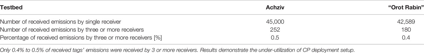
Table 1 Records of successful tag detections from Achziv Marine Nature Reserve tracking 19 slipper lobsters for a period of 8 month, and from “Orot Rabin” Power and Desalination Station testbed tracking 20 sandbar sharks for a period of 87 days.

The problem of how to position receiving nodes resembles the “Art gallery problem” (Rajagopal et al., 2016), whose goal is to find the minimal set of guards such that every point in a floor plan is covered by at least one guard. In the case of 2D localization, three receivers represent a guard. While this type of optimization problem is proven to be NP-Hard (nondeterministic polynomial time hard) (Lee and Lin, 1986), i.e., the complexity of search increases with the problem size in such a way that a solution would compare with the brute-force approach of trying out the entire state-space, some work-arounds are possible. For indoor localization, information about the floor plan is utilized to reconcile position ambiguities formed by the localization of a node by only two receivers (Rajagopal et al., 2016). The proposed method disqualifies potential positions located outside the floor or behind barriers/walls that block the signals. To manage spatial-dependent propagation loss in indoor localization, templates of the reception pattern are used (Mnasri et al., 2015) as well as modeled calculations (Rajagopal et al., 2016). However, the solution for underwater localization is somewhat different. First, while the sea includes barriers that can be used to resolve localization ambiguities, these mostly apply in near shore locations. Furthermore, while some solutions relied on the structure of the seabed for localization, e.g., in Dubrovinskaya et al. (2017), localization accuracy is low if the structure is not diverse.

In this paper, we propose a systematic method to determine the deployment setup of a marine fauna tracking testbed considering the acoustic specifications of the tags, the number of receivers, and the environmental properties. As a test case, we consider 16 mm tags that are suitable for tagging megafauna. Relying on prior knowledge of the bathymetric and bathythermal conditions in the explored area, we formalize a constraint optimization problem that accounts for the spatially dependent propagation loss, and yields the best deployment locations to maximize the coverage area. In our analysis, we consider the user’s area-of-interest, I,and evaluate the coverage quality by the geometrical dilution of precision (GDOP) (Sharp et al., 2009). Since I may be non-convex, the optimal solution is often NP-hard, i.e. to solve the decision problem of “where to position the receivers?” requires unreasonable long time such that even for a modest I the solution becomes too hard to evaluate. For these cases, we offer a sub-optimal implementation based on a genetic algorithm (GA). We refer to our approach as the Propagation-Dependent Anchor Deployment (PDAD) scheme. For simple setups, we show that PDAD achieves the optimal solution, as verified by a brute force search. For more complex setups, we compare the coverage area yielded by PDAD to that of CP.

Our contribution is twofold:

1. A novel systematic approach and optimization formalization for how to set up the location of anchored receivers in an underwater testbed.

2. A method to merge the GDOP metric with bathymetric information to quantify detection ranges.

We explore the performance of our method in numerical simulations and in a sea experiment. The former demonstrates the obtained deployment strategy for three different seabed environments and explores the sensitivity of the results to the system’s parameters, as well as the degree of sub-optimality of the proposed solution. The latter demonstrates the merit of using the proposed approach in a real sea environment as a test case for tracking megafauna. Compared to the CP strategy, the results show an increase of roughly 30% in the size of the covered area as obtained by PDAD.

Materials and Methods

In this section, we describe our system model and formulate our solution. We use the following notations: coordinates are marked by a macron sign, e.g. I sets are marked by bold letters, e.g., D_i. Table 2 summarizes the paper’s main variables and notations.

TABLE 2

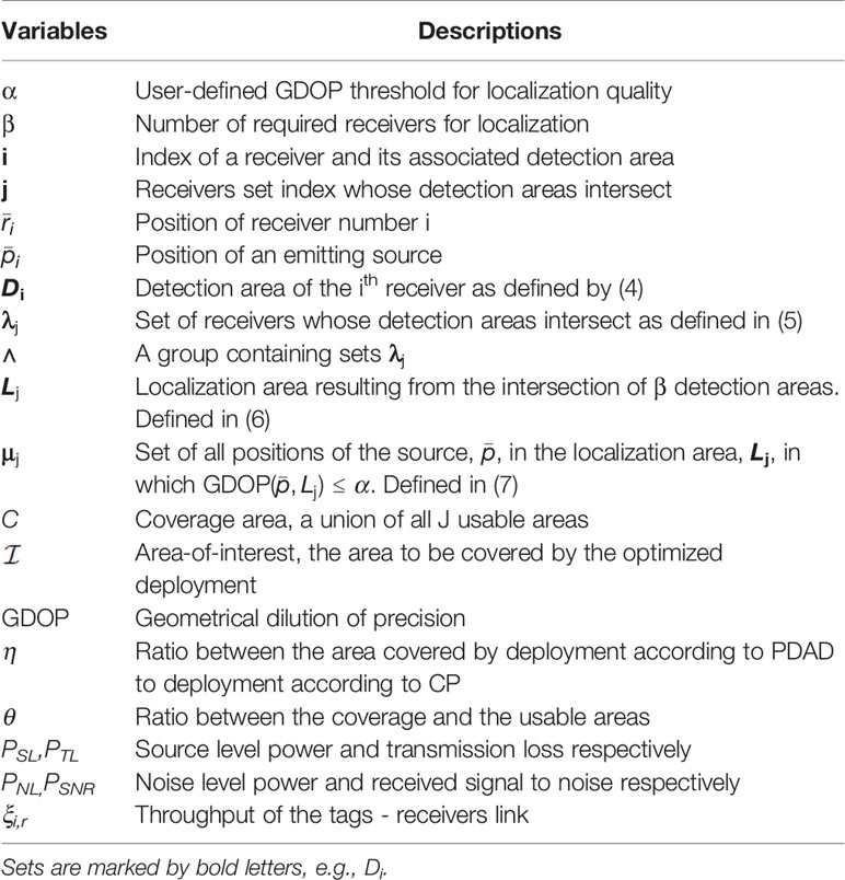
Table 2 Main variables and notations - Coordinates’ variables are marked by a macron sign, e.g., $\overline{p}$.

Study Area

Our setup includes N receivers deployed to cover a given area-of-interest . Our goal is to determine the optimal location and deployment depth for the receivers, such that a tagged animal that passes through  is well-localized within area  and possibly beyond it. For each tag’s emission, the detecting receiver measures the local arrival time, such that, assuming all N receivers are time-synchronized, localization is performed by TDoA cf. (Alexandri et al., 2018).

We assume prior knowledge to evaluate the propagation loss between any pair of positions within and beyond . In particular, we require information about the bathymetry within the explored area and the expected bathythermal profile of the water. This information is used to run a propagation loss model such as ray-tracing, normal modes, or parabolic equation (Bahrami et al., 2016; Gul et al., 2017). We admit that, since the bathythermal profile is time varying and depends on seasons, the sound velocity profile (SVP) cannot be accurately known for the entire deployment time period. Yet, a track of the bathythermal profile may reveal temporal trends in the sound speed, allowing the evaluation of a nominal SVP. Alternatively, the user may perform periodic measurements of the bathythermal and change the locations of the receivers if needed.

Detection Range

Let P_SL be the source power level of the tag to-be-localized. Let P_NL be the ambient noise level, assumed constant in the explored area, and let be$P_{\text{TL}}\left({\overline{r}}_i,\overline{p}\right)$ the power transmission loss between a source node at position $\overline{p}=\left(x,y,z\right)$ and the ith receiver at position ${\overline{r}}_i=\left(x_{\text{i}},y_{\text{i}},z_{\text{i}}\right),\text{ i}=1,2,\dots ,\text{N}$. We calculate $P_{\text{TL}}\left({\overline{r}}_i,\overline{p}\right)$ and P_NL by acoustic channel modeling, i.e., modeling the acoustic attenuation by considering the environmental conditions, the ambient noise, and the emitted frequency, e.g., (Gul et al., 2017), and from the Wenz curves for acoustic ambient noise in the ocean (National Research Council, 2003), showing the average ambient noise spectra for different levels of shipping traffic, and sea state conditions. Specifically, analyzing a huge set of acoustic measurements of ambient noise, Wenz was able to provide an empirical curve for the ambient noise level and to show that it is frequency and environment dependent. Then, comparing the received level

$\begin{array}{ll}{P}_{\text{SNR}}=\frac{P_{SL}\times P_{\text{TL}}\left({\overline{r}}_i,\overline{p}\right)}{P_{NL}}& (1)\end{array}$

to a detection threshold, P_DT, we measure whether location ${\overline{r}}_i$ is suitable for detecting a source located at $\overline{p}$. That is, if P_SNR ≥ P_DT a receiver positioned at ${\overline{r}}_i$will detect a tag emitting at $\overline{p}$

Localization Quality

A common metric to measure the achievable localization accuracy for the planned receivers’ deployment is the GDOP. This is a unitless metric that ranks the deployment setup by considering both the measurement precision and the geometry between the source and receivers to account for the effect of the geometry setup on localization (Kaplan and Hegarty, 2005). As localization quality improves, the GDOP decreases. Classification of GDOP values are outlined in Table 6. For example, if all receivers are colinear, the achievable localization quality is poor. Given a set $\lambda =\left\{{\overline{r}}_1,\overline{r},\dots ,{\overline{r}}_N\right\}$ of N receivers stationed at locations, $\left\{{\overline{r}}_1,\overline{r},\dots ,{\overline{r}}_N\right\}$ the GDOP is defined as the ratio between the accuracy of a position fix to the variance of the measurements (Sharp et al., 2009). Formally, denote the visibility matrix (Yarlagadda et al., 2000; Kaplan and Hegarty, 2005)

$\begin{array}{ll}H\left(\overline{p},\lambda \right)=\left[\begin{array}{llll}{a}_{\text{x}1}\hfill & a_{\text{y}1}\hfill & a_{\text{z}1}\hfill & 1\hfill \\ a_{\text{x}2}\hfill & a_{\text{y}2}\hfill & a_{\text{z}2}\hfill & 1\hfill \\ a_{\text{x}3}\hfill & a_{\text{y}3}\hfill & a_{\text{z}3}\hfill & 1\hfill \\ ⋮\hfill & ⋮\hfill & ⋮\hfill & ⋮\hfill \\ a_{\text{xN}}\hfill & a_{\text{yN}}\hfill & a_{\text{zN}}\hfill & 1\hfill \end{array}\right]& (2)\end{array}$

whose elements are the unit vectors pointing from a potential position of the source, $\overline{p}=\left[p_{\text{x}},p_{\text{y}},p_{\text{z}}\right]$, to the location of the i^th receiver, $\overline{r}=\left[r_{{\text{x}}_{\text{i}}},r_{{\text{y}}_{\text{i}}},r_{{\text{z}}_{\text{i}}}\right]$ ,such that, a_xi=(p_x−r_xi)/R_i,a_yi=(p_y−r_yi)/R_i and, a_zi=(p_z−r_zi)/R_i where, $R_{\text{i}}=\sqrt{{\left(p_{\text{x}}-r_m{x}_i\right)}^2+{\left(p_{\text{y}}-r_{{\text{y}}_{\text{i}}}\right)}^2+{\left(p_{\text{z}}-r_{{\text{z}}_{\text{i}}}\right)}^2}$ all in Cartesian coordinates. The $\text{GDOP}\left(\overline{p},\lambda \right)$ equals, $\sqrt{{\mathfrak{g}}_{11}^2+{\mathfrak{g}}_{22}^2+{\mathfrak{g}}_{33}^2+{\mathfrak{g}}_{44}^2}$, where

$\begin{array}{ll}{\left(H^{\text{T}}H\right)}^{-1}=\left[\begin{array}{llll}{\mathfrak{g}}_{11}\hfill & {\mathfrak{g}}_{12}\hfill & {\mathfrak{g}}_{13}\hfill & {\mathfrak{g}}_{14}\hfill \\ {\mathfrak{g}}_{21}\hfill & {\mathfrak{g}}_{22}\hfill & {\mathfrak{g}}_{23}\hfill & {\mathfrak{g}}_{24}\hfill \\ {\mathfrak{g}}_{31}\hfill & {\mathfrak{g}}_{32}\hfill & {\mathfrak{g}}_{33}\hfill & {\mathfrak{g}}_{34}\hfill \\ {\mathfrak{g}}_{11}\hfill & {\mathfrak{g}}_{22}\hfill & {\mathfrak{g}}_{33}\hfill & {\mathfrak{g}}_{44}\hfill \end{array}\right].& (3)\end{array}$

Problem Statement

To formulate the receivers’ deployment problem, four sets of variables are required. Recall that the source node is detected when $P_{\text{DT}}\left({\overline{r}}_{\text{i}},\overline{p}\right)\le P_{\text{SL}}\times P_{\text{TL}}/P_{\text{NL}}$. We define the detection area, D_i, as the set of all possible positions of the source such that a receiver located at ${\overline{r}}_{\text{i}}$ will detect the source’s transmissions. Formally,

$\begin{array}{ll}\overline{p}\in D_{\text{i}}|P_{\text{DT}}\left({\overline{r}}_i,\overline{p}\right)\le \frac{P_{SL}\times P_{\text{TL}}\left({\overline{r}}_i,\overline{p}\right)}{P_{NL}}& (4)\end{array}$

The resolution of set D_i is determined by the resolution of the bathymetric information. An example of a detection area for four receivers is shown in Figure 1A. Note that the detection area obtained is not necessarily convex. Let ∧β be a group containing sets λ_j, j=1,…,J,where λ_j is the jth set of at least β receivers whose detection areas intersect such that

$\begin{array}{ll}{\lambda }_{\text{j}}\in \text{Λ}\left(\beta \right)\mid {\displaystyle \underset{\text{i}\in {\lambda }_{\text{j}}}{\cap }{D}_{\text{i}}\ne \varnothing ,}|{\lambda }_{\text{j}}\mid \ge \beta .& (5)\end{array}$

FIGURE 1

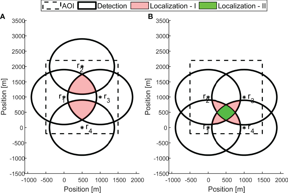
Figure 1 An example showing the deployment of N = 4 receivers ${\overline{r}}_1,{\overline{r}}_2,{\overline{r}}_3,{\overline{r}}_4$, with corresponding detection areas marked by black contour lines. For the case of β = 3, in deployment setup (A), although J = 5, there are two localization areas, L(λ₁), L(λ₂), marked by the light red shading. The two sets of at least 3 receivers are ${\lambda }_1=\left\{{\overline{r}}_1,{\overline{r}}_2,{\overline{r}}_3\right\}$ and ${\lambda }_2=\left\{{\overline{r}}_1,{\overline{r}}_3,{\overline{r}}_4\right\}$ . The coverage area, C, is the union of L( λ₁ ), L( λ₂ ) . In the deployment setup (B), the light red areas form “Localization area - I”, which merges localization areas L( λ₁ ), L( λ₂ ) ,  L( λ₃ ), L( λ₄ ) for which β = 3 detection areas overlap. The light green areas form “Localization area - II”, for which β = 4 detection areas overlap. For both deployment setups, the resulting localization area is non-convex.

For example, β = 3 for 2D localization¹, and β =4 for 3D localization. As shown in Figure 1A, for β =3, there are two sets of 3 receivers, { r₁, r₂, r₃ }∈ λ₁ { r₁, r₃, r₄ }∈ λ₂.The group containing all the sets is { λ_1, λ₂} ⋲∧(β).

For a given λ_j, we define a localization area, L_j (λ_j, β) ,as an area resulting from the intersection of at least β detection areas. Formally,

$\begin{array}{ll}L\left({\lambda }_{\text{j}},\beta \right)={\displaystyle \underset{\text{i}\in {\lambda }_j}{\cap }{D}_{\text{i}}|{\lambda }_{\text{j}}\in \text{Λ}\left(\beta \right).}& (6)\end{array}$

Denote a usable area, U_j (λ_j, β), as the set of all positions of the node to be localized, $\overline{p}$, in the localization area L(λ_j, β) for which “good” localization is attainable. Specifically, the usable area is an area for which,$\text{GDOP}\left(\overline{p},L_{\text{j}}\left({\lambda }_j,\beta \right)\right)\le \alpha$ where α is a scalar value determined by e.g., Table 6. Formally,

$\begin{array}{ll}\overline{p}\in {\mathcal{U}}_{\text{j}}\left({\lambda }_j,\beta \right)\mid \text{ GDOP}\left(\overline{p},L_{\text{j}}\left({\lambda }_j,\beta \right)\right)\le \alpha ,\overline{p}\in L_{\text{j}}\left({\lambda }_j,\beta \right).& (7)\end{array}$

Our fourth set is the coverage area, C(β) ,denoted as the union of all usable areas,

$\begin{array}{ll}C\left(\beta \right)={\displaystyle \underset{\text{j}}{\cup }{U}_{\text{j}}}\left({\lambda }_j,\beta \right).& (8)\end{array}$

We formulate the task of receiver deployment as an optimization problem whose solution is locations, ${\overline{r}}_{\text{i}}, \text{i}=1,\dots ,N$ .which maximize the size of the coverage area‖ C ‖:

$\begin{array}{ll}\begin{array}{c}\underset{r_1,r_2,\text{...}{r}_{\text{N}}}{\text{argmax}}\Vert C\left(\beta \right)\Vert \\ \text{st. }\Vert C\left(\beta \right){\displaystyle \cap I}\Vert \ge \rho \Vert I\Vert .\end{array}& (9)\end{array}$

Since most applications require the coverage of a given area of interest, I, we constrain the solution such that the resulting convergence area covers at least p percent of I. This constraint also allows for the discrimination between a “must-be-covered” area and a “nice-to-have” coverage area. An example of such a consideration is presented in (Pickholtz et al., 2018) for the monitoring of acoustically-tagged herbivorous fish, Siganus rivulatus, close to the shore area. In this case, the movements of the herbivorous fish close to the shallow fringing coral reefs are of interest (the “must-be-covered” area), along with information from other areas along the shore (the “nice-to-have” area).

The PDAD Approach

Optimal Formalization

We formulate the problem statement in (9) as a mixed constraint optimization problem. In accordance with (9), let I, D, LU and C be 3D matrices representing the area-of-interest, the detection area, localization area, usable area, and the coverage area, respectively. The matrices’ rows, columns, and depths represent the quantized x, y, z grid in Cartesian coordinates, with lower-case letters representing the matrix entries with a resolution set by the bathymetry information (e.g., every 5m). For example, entry is the entry of i^K×L×M. The capability to detect a source located in position $\overline{p}\left(x=k,y=l,z=m\right)$ by the i^th receiver located in position ${\overline{r}}_i$ is defined by the binary operator

$\begin{array}{ll}{d}_{\text{k},\text{l},\text{m}}\left({\overline{r}}_i\right)=\{\begin{array}{ll}1\hfill & \text{f }{P}_{\text{DT}}\left(\overline{p}\left(k,l,m\right),{\overline{r}}_i\right)\le \frac{P_{SL}\times P_{TL}}{P_{NL}}\hfill \\ 0\hfill & \text{ otherwise}\hfill \end{array}& (10)\end{array}$

Then, a source located in position $\overline{p}$ can be localized if it is detected by at least β receivers. The elements of L (λ_j, β) are formalized by the binary operator

$\begin{array}{ll}{l}_{\text{k},\text{l},\text{m}}\left({\lambda }_{\text{j}}\right)=\{\begin{array}{ll}1\hfill & {\displaystyle \sum _{\text{i}=1}^N{d}_{\text{k},\text{l},\text{m}}\left({\overline{r}}_i\right)\ge \beta ,\overline{r}\in {\lambda }_{\text{j}}}\hfill \\ 0\hfill & \text{otherwise\hspace{0.17em},}\hfill \end{array}& (11)\end{array}$

where each λ_j is a subset of, ∧(β) containing at least β receivers. Here, ∧(β) is the complete set of ${\overline{r}}_i$ receivers i = 1,…,N. Note that the maximum number of such λ_j sets is $J={\displaystyle \sum _{\text{p}=\beta }^N\left(\underset{p}{\overset{N}{\hspace{0.17em}}}\right)}$.

Recall that the usable area U_j is the mapping of all locations $\overline{p}$ inside L (λ_j, β) whose GDOP is smaller than a given threshold α. In the matrix representation,

$\begin{array}{ll}{u}_{\text{k},\text{l},\text{m}}\left({\lambda }_{\text{j}},\left(\beta \right)\right)=\{\begin{array}{ll}1\hfill & \text{GDOP}\left(L_{\text{j}}\left({\lambda }_j,\beta \right)\right)\le \alpha \hfill \\ 0\hfill & \text{otherwise\hspace{0.17em}}.\hfill \end{array}& (12)\end{array}$

Similarly, the coverage area matrix, defined as the union of all the different usable areas j = 1 …J, is formalized by the binary operator

$\begin{array}{ll}{c}_{\text{k},\text{l},\text{m}}\left(\beta \right)=\{\begin{array}{ll}1\hfill & \text{f }{u}_{\text{k},\text{l},\text{m}}\left(\text{Λ},\left(\beta \right)\right)=1\hfill \\ 0\hfill & \text{otherwise\hspace{0.17em}}.\hfill \end{array}& (13)\end{array}$

The intersection of C(β) and J in the constraint of (9) can thus be expressed by

$\begin{array}{ll}\Vert C\left(\beta \right){\displaystyle \cap I}\Vert ={\displaystyle \sum _k{\displaystyle \sum _l{\displaystyle \sum _m{c}_{\text{k},\text{l},\text{m}}\left(\beta \right)i_{\text{k},\text{l},\text{m}}.}}}& (14)\end{array}$

Note that d_k,l,m, l_k,l,m , c_k,l,m are all a function of locations ${\overline{r}}_i,\dots ,{\overline{r}}_N$ which in turn can take any value within C and whose determination is the goal of this work. The deployment is obtained by solving

$\begin{array}{ll}\text{Λ}=\underset{{\overline{r}}_i,\dots {\overline{r}}_N}{\text{argmax}}{\displaystyle \sum _k{\displaystyle \sum _l{\displaystyle \sum _m{c}_{\text{k},\text{l},\text{m}}}}}& \text{(15a)}\end{array}$

$\begin{array}{ll}\text{s.t.\hspace{0.17em}\hspace{0.17em}}{\displaystyle \sum _k{\displaystyle \sum _l{\displaystyle \sum _m{c}_{k,l,m}{i}_{k,l,m}}}}\ge \rho {\displaystyle \sum _k{\displaystyle \sum _l{\displaystyle \sum _m{i}_{k,l,m}}}}& \text{(15b)}\end{array}$

Algorithmic Solution

A closed-form solution of (15) for the simple case of three receivers deployed over a flat seabed with isotropic propagation loss is presented in the Appendix. We note that, in the general case, problem (15) is non-convex. This is because, as illustrated in Figure 1, even when the detection area of each receiver is convex (a circle or an ellipsoid) - and thus so is the localization area - the coverage area may be constructed from a number of non-continuous usable areas. Furthermore, as demonstrated in Figures 1A, B, even for a convex localization area, the usable area itself may be non-convex. Hence, (15) is a constrained non-convex optimization problem, which can be solved by procedures such as branch and bound (B&B) (Clausen, 1999) with a polynomial complexity on average (Zhang and Korf, 1992; Shabi et al., 2017), or by randomized approaches such as simulated annealing (Blum et al., 2021). Here, we propose to use GA, which is suitable for complex deployments, i.e., a larger number of receivers and diversified bathymetric and bathythermal conditions. We chose GA since it is suitable for overcoming local minima in problems involving a non-convex objective function (Mnasri et al., 2015). The fitness function is multi-objective, seeking to maximize the coverage area inside I and to minimize a penalty function for coverage outside I.

Evolutionary algorithms (EA) have probabilistic convergence time (Ankenbrandt, 1991). The average convergence time is defined as the number of generations it takes to reach convergence (Rylander, 2001). To that end, the complexity depends on the individual’s and population’s representation, the implementation of mutation, crossover and selection processes, and the fitness function (Corus et al., 2017). Given the above, the complexity is on the order of, where g is the number of generations, p is the population size, and i is the size of the individuals. We implemented PDAD using Python’s “DEAP” evolutionary computation framework package and used it both for the simulation and the sea experiment.

Numerical Investigation Setup

To analyze PDAD performance, we consider three environments with different attributes:

1. A theoretical, simple environment: a flat seabed with an isotropic SVP, termed SVP_ISO. This type of environment may be considered when the environmental conditions are unknown.

2. A moderate spatially diverse area: an area of 6000 × 6000 m² shallow water area close to the “Orot Rabin” Power and Desalination Station in Hadera, Israel (32°28’N; 34°52’E; an area we also explored in our sea experiment. Within this area, the selected I area is a 2000 × 2000 m² rectangle with a water depth ranging from 0 to 25 meters. The entire area was divided into a grid of 60 × 60, yielding a sample resolution of 100 m. Here, the receivers are anchored at a depth of 0.5 m above the seabed, and the mobile transmitter moves at a depth of 3 m. The bathymetry of this area is shown in Figure 2A.

3. An extremely diverse seabed: a coastal area north of San Diego between 32.65°N to 32.755°N and -117.265°-117.265° W and -117.35 117.35° W (Divins and Metzger, 2021). Out of this 5000 × 4000 m² area, we picked I to be a square of 3000 × 3000 m², which was divided into grid cells of a 100 m resolution. For this environment, the simulated receivers are anchored at a depth of 2 m above the seabed, while the mobile node maintains its depth at 10 m. Figure 3A shows the bathymetry of the considered area, and its SVP is shown in Figure 3B. The diversity of the considered area is demonstrated in Figures 3C, D, showing significant differences between the effective detection area for two different grid positions.

FIGURE 2

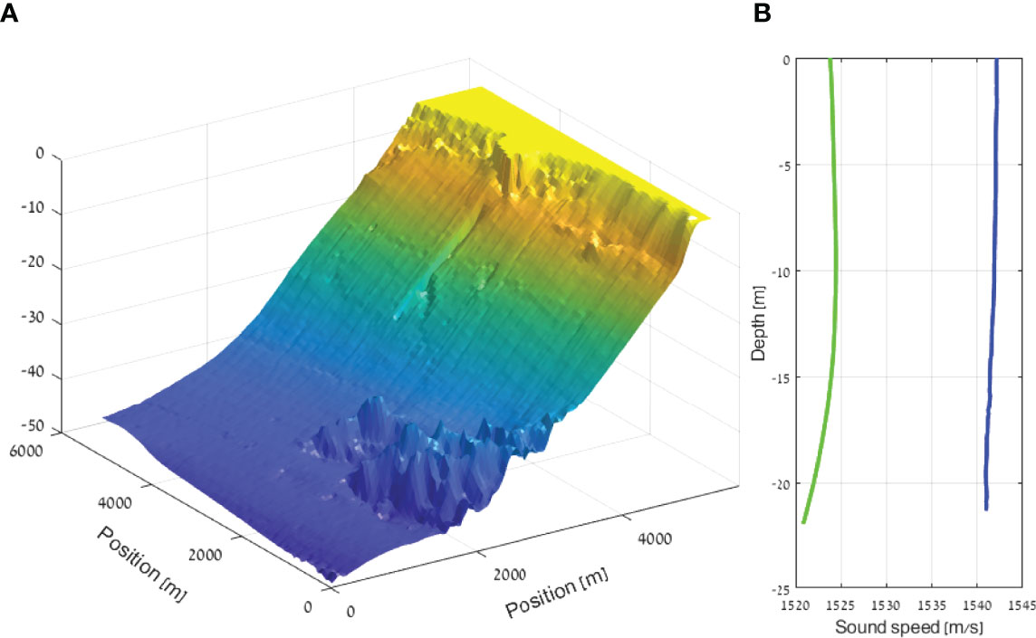
Figure 2 (A) Bathymetry, (B) eastern Mediterranean winter SV, SVP_H (blue) measured sea experiment SVP_M (green) of the area near “Orot Rabin” Power and Desalination Station in Hadera, Israel.

FIGURE 3

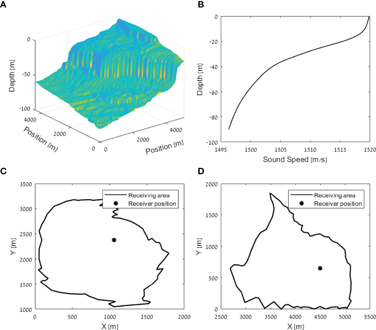
Figure 3 Environmental condition of shallow water close to San Diego Bay. (A) Bathymetry and (B) the sound velocity profile. The impact on the expected detection area of a single receiver is shown in (C) for a receiver positioned at (1000, 2400, -10) and in (D) for a receiver positioned at (4500, 750, -10).

We consider the specification of an actual acoustic tag manufactured by Thelma-Biotel Inc., Trondheim, Norway (Alexandri et al., 2018). These acoustic tags are used globally in applications to monitor fauna in marine environments and to track migration patterns (Lennox et al., 2021; Reubens et al., 2021). The mobile node is an acoustic tag (model: ID-HP16) emitting 69kHz single-tone signals of intensity 158dB re 1μPa @ 1m. A range test we performed showed that the detection distance is 1000m in shallow water with a sandy bottom (Alexandri et al., 2019).

To measure the GDOP in each deployment setup, the spatial-dependent propagation loss must be accounted for. We consider two ways to attain the propagation loss. The first, assigned only in the case of a flat seabed with an isotropic SVP, applies a transmission loss model of

$\begin{array}{ll}\text{TL}=10\text{log }(R)+\alpha R/1000,& (16)\end{array}$

with R being the transmission range and α the absorption parameter. The result is a transmission power loss of 48dB, where α = 18 dB/km for 69 kHz (Urick, 1983). For complex environments, we consider the Bellhop ray-tracing propagation model (Porter, 2011). In both cases, the detection area is calculated by setting a limit on the signal-to-noise ratio to be above 10 dB.

For each of the above three areas, two types of deployment setups were compared. The first is based on the CP method of positioning the receivers at the vertices of equilateral triangles partially covering the inner area of I .The distance between the receivers is set to half of the tags’ specified detection range, namely 500 m. The second deployment setup is based on positioning the receivers according to the PDAD. Each individual is a set of the receivers’ coordinates x and y. For the GA sub-optimal solution, the initial population size is based on a single individual positioned at the center of I with the rest of the individuals positioned around the center position. The effectiveness of the two methods is compared in terms of the size of the resulting coverage area for each deployment strategy. To this end, we chose the coverage area to be such that for each point inside I , DOP ≤ 5.

In our simulations, we used an AMD Ryzen™ Threadripper™ 3990X CPU with 128 threads and measured processing time of about 100 msec per thread per each possible deployment setup. To evaluate the complexity of the proposed deployment scheme, we note that the size of a search space to position N receivers in a given area divided into a rectangular grid of x × y is (xy)^N. For example, for a grid size of 100 × 100 and N = 3, the search space sizeis 10¹². Hence, with the full utilization of our server, a complete search of the search space will last more than 24 years. This is because of the complexity of a solution in which brute-force searches the considered area is O((xy))^N.In our case, using the PDAD approach, the best solution for the flat bottom isotropic propagation environment was achieved in the range of 500 to 2700 GA’s generations for the different available number of receivers. Using a 64 core, 128GB memory computer, the processing time was 2:30 hours for 3 receivers deployment and 28 hours for 10 receivers deployment.

Sea Experiment Setup

The sea experiment aimed to demonstrate the applicability of our simulation results, and to explore the benefit of the proposed PDAD strategy in the realistic case of a low-resolution possibly-mismatched bathymetry map. The experiment took place in November 2021 close to the “Orot Rabin” Power and Desalination Station in Hadera, Israel (32°28’N; 34°52’E), in an area of interest of 1200 × 1400 m², at the southeastern part of the same area used in one of our numerical analysis cases (see the bathymetry map in Figure 2). We used acoustic equipment from Thelma Biotel AS., Trondheim, Norway - specifically, 7 acoustic tags and the standard receivers that decode these emissions. The experiment involved four kayaks, each was towing a small buoy 2 m behind its stern. The tags were attached roughly 2 m below the buoy, and maintained their depth using a balancing weight attached below the tags. For groundtruthing, each kayak carried a GPS receiver that logged its location throughout the trial. Two clusters of four receivers each were anchored at a depth of 1 meter above the seabed in the explored area. One cluster was positioned according to the CP approach, and the other according to the results of a PDAD calculation using a given bathymetry map of the area and an SVP measured prior to the experiment. The measured SVP, SVP_M, is shown in Figure 2B.

In addition to comparing the size of the usable area for CP and PDAD, a second performance metric explored the throughput of the tags - receivers link, defined as ξ_i,r. Here, the throughput is defined by the ratio between the number of receptions to the total number of emissions. Specifically, two cases are considered. 1) ξ2,r is the ratio between the number of received emissions by one or two receivers and the total number of emissions, and 2) ξ3,r it the ratio between the number of received emissions by three or four receivers and the total number of emissions throughout the experiment. The former reflects on the detection properties of the deployed setup, while the later on the localization quality. The throughput metric accounts for possible uneven time spent by the kayaks in the CP or PDAD setups. To avoid bias, we normalized the throughput by the tags’ distances to the center of each area. Specifically, for each cluster of four receivers, the geometric center of the area was calculated. Then, the throughput was calculated and normalized by the tag’s range from the cluster centroid.

Figure 8 shows the receivers’ locations in the explored area. The position of the CP’s receivers are marked by aqua-colored squares, and the positions of the PDAD’s receivers are marked by red-colored diamonds. In a previous work (Alexandri et al., 2019), a range test showed that in the considered environment, the detection range of a similar tag and receiver pair is roughly 1,000 m. Thus, for CP, the distance between the receivers was set to 500m. We note that both CP and PDAD shared receiver number 2.

The experiment lasted for 240 min. During that time, each tag emitted a signal in a fixed interval every 30 to 45 sec, for a total of 2,730 emissions. Out of these, 406 emissions were detected by at least one receiver and 280 emissions were detected by at least three receivers of the CP or PDAD clusters. In order to ensure that the four kayaks cover the complete area of interest, their route, provided in Figure 8, was planned to reach beyond the anticipated detection range of the tags. As a result, we report low tag detection rate. For each detected emission, the receivers measured the ToA by their internal clock. The receivers were time-synchronized prior and after the experiment. This involved both synching the receivers’ clock to a reference clock by attaching a specific acoustic tag to one of the receivers, and using its emissions to time-synchronize the others (see details in (Alexandri et al., 2018)). Tag emissions were sorted and aggregated to the CP and PDAD clusters. If received by either three or four receivers, the emissions were considered to be inside the usable area that allows localization. To comment on the receiving conditions we also recorded the ambient noise level, as measured by each receiver.

Results

In this section, we report results from the numerical investigation of our deployment method and from the designated sea experiment. For the simulations, we used the size of the area which achieves good localization, i.e., GDOP ≤ 5, and explored the results against the brute-force solution and compared to CP. We also investigated the sensitivity to the system’s parameters - in particular, the number of receivers, the size of C for different GDOP values, and to different SVPs. For reproducibility, we shared our implementation code in the Supplementary Material.

Simulation Results

We start by analyzing the results of the theoretical environment. Figure 4 shows the size of C (β =3) for the case of three receivers as a function of the distance between the receivers, l, normalized by their receiving range, R. The maximum coverage area for GDOP=5 is attained when the distance between the receivers is about half of the receiving range. For cases of higher GDOP values, i.e. the localization accuracy in some parts of C is of lower quality, a larger coverage area can be attained. For example, for GDOP=8, the optimal distance between the receivers is about 40% of the receiving range and C =1.85R². For a lower GDOP, when localization accuracy is of high priority, a smaller coverage area is attainable. For example for GDOP = 2 the maximal attainable coverage area is C =1.14R² for l = 0.66. This result may serve as a guideline for deployments in non-spatially diverse areas. The analytical derivation of the attainable coverage area for the theoretical environment is outlined in the Appendix and in Figure 10. In Figure 5, we compare the achieved coverage area between CP and PDAD for different numbers of receivers, ranging from 3 to 13. We observe that the coverage area gained by using PDAD over CP increases with the number of receivers. This is attributed to the increase in the number of degrees of freedom for the receivers’ placement.

FIGURE 4

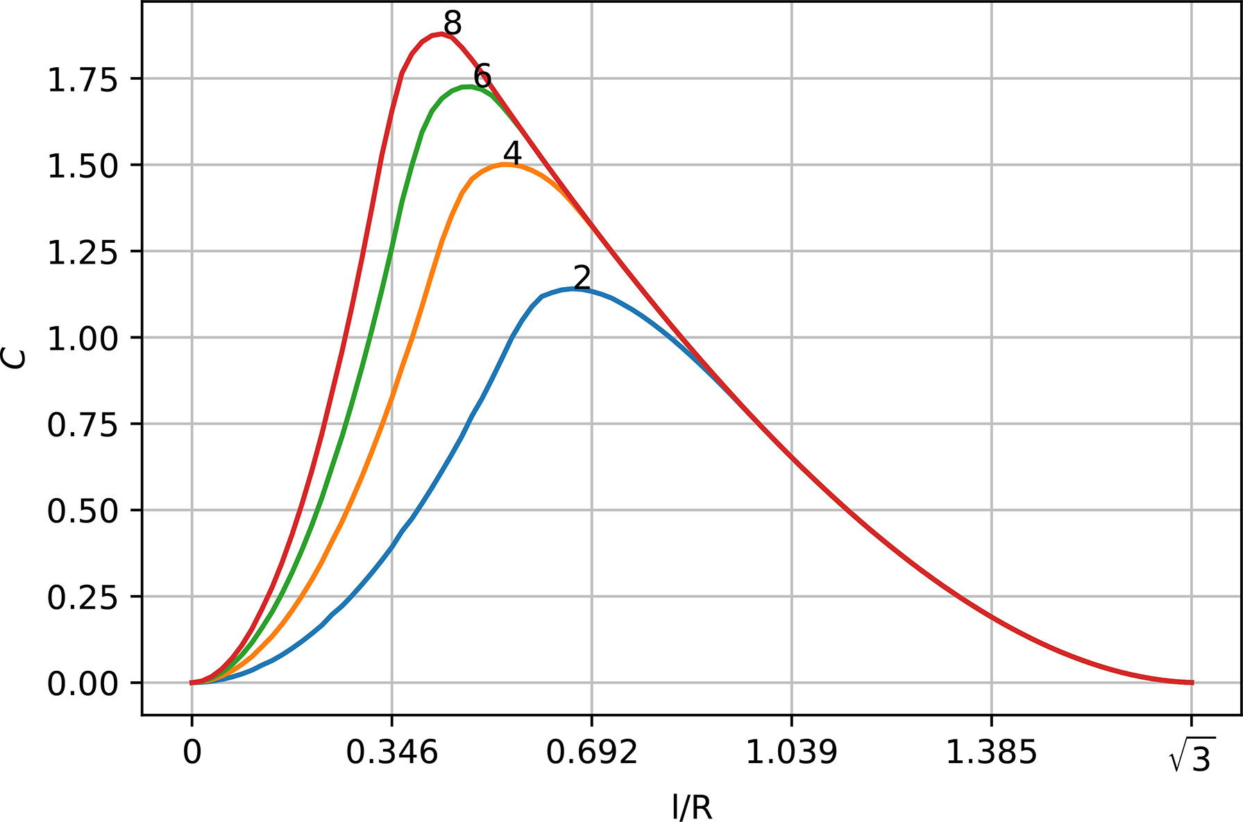
Figure 4 Effect of distance between the receivers, I/R, normalized to the maximum receiving range, R, on covered receiving area, C, and attained positioning quality for 3 equilateral receivers’ deployment in isotropic propagation loss. As the quality of positioning increases (the GDOP is smaller), the attained covered area C decreases.

FIGURE 5

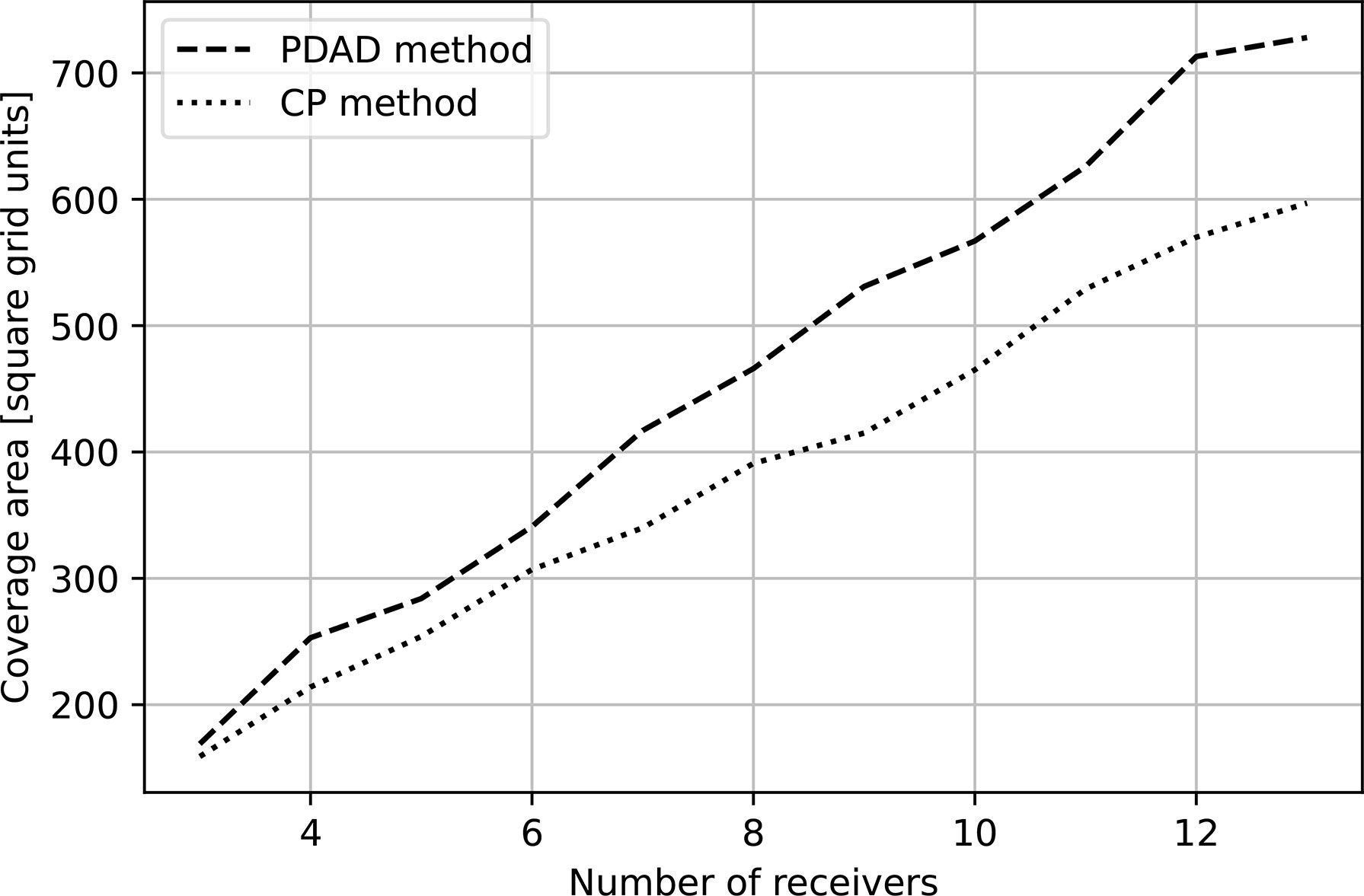
Figure 5 Area covered by deployment setup based on CP method, i.e., positioning the receivers at the vertices of equilateral triangles vs. deployment based on the proposed PDAD method, i.e., optimization of receivers locations based on the surrounding environmental conditions.

For the moderate spatially diverse area, in Table 3, we compare the results for two SVPs: a simple fixed profile of 1520 m/s, SVP_ISO, and an eastern Mediterranean winter SVP, as shown in Figure 2B (Salon et al., 2003), termed SVP_H. The first two columns of Table 3 summarizes the ratio between the size of the coverage area as obtained by PDAD and CP, for the moderate diverse bathymetry in Hadera

$\begin{array}{ll}\eta =C_{\text{PDAD}}/C_{\text{CP}}.& (17)\end{array}$

TABLE 3

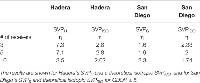
Table 3 η - from (17) for deployment of 3, 5 and 10 receivers at the Hadera power station and in San Diego.

The results are presented in Table 3 for the different number of receivers, and for GDOP ≤ 5. We observe that, using PDAD, for both SVPs the attainable covered area is larger than that of CP. An interesting result presented in Figure 6 shows that for the deployment of 5 receivers in isotropic conditions - in contrast to CP where all of the receivers are placed inside I- the PDAD solution suggests that 3 out of the 5 receivers be placed outside I. This deployment yields an increase of 67% in the localized area. Finally, from the results in Table 3, we observe the difference of the gain obtained for the two different SVPs. A much higher gain in using PDAD is shown when the SVP is complex. This is because a diverse SVP impacts the propagation loss, rendering the channel to be spatial dependent.

FIGURE 6

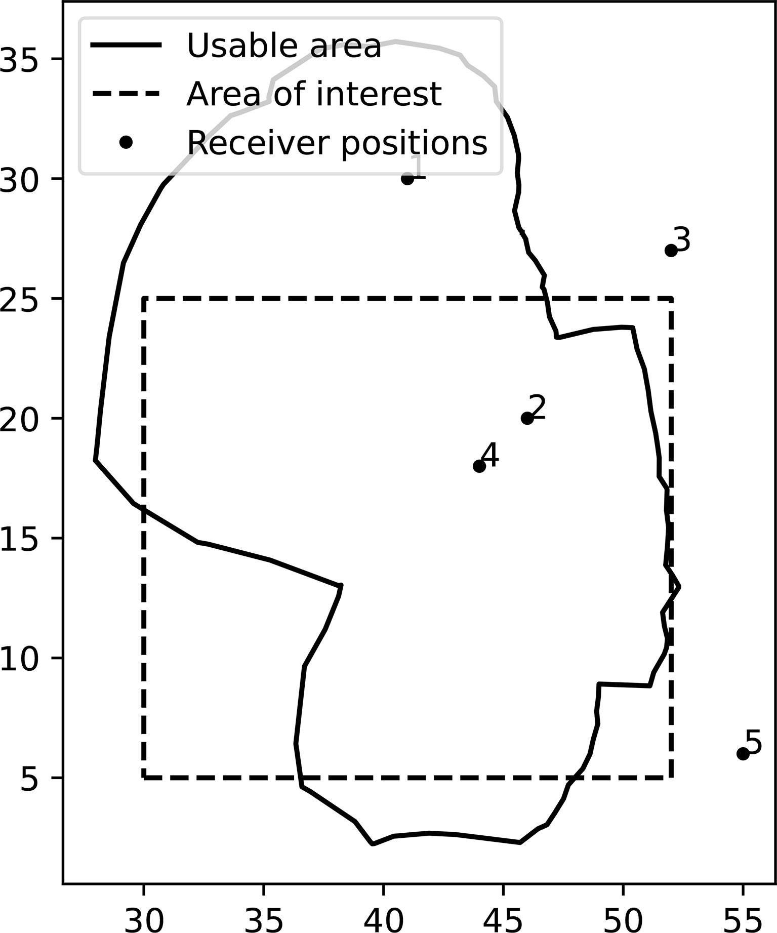
Figure 6 Usable area for the deployment of 5 receivers in isotropic SVP, SVP_ISO ,in a moderate spatially diverse area. Note that 3 out of the 5 receivers are positioned outside of I.

The third and fourth columns of Table 3 show the values of η from (17) for the third explored environment with the highly diverse bathymetry (the San Diego area) for its SVP_S and a theoretical isotropic SVP_ISO. We observe that the size of the coverage area obtained by PDAD is also significantly larger than that of CP in the case of complex bathymetry. We note that the marginal added coverage area for the SVP in San Diego increases with the number of receivers but an opposite trend is shown for the Hadera area. This is due to the higher diversity of the San Diego seabed and due to the deployment strategy. The former is attributed to bathymetry complexity. That is, when the bathymetry is highly complex, e.g., the one from San Diego, adding receivers helps cover shadow zones and their proper deployment location becomes more important. In less complex environments, e.g., the one from Hadera, adding receivers helps CP cover more area for localization and the gain in using PDAD decreases. We observe that the performance gain in the Hadera area increases for the more complex SVP, but the performance gain in the San Diego area is higher for the isotropic SVP. We explain this by the randomness of the CP method. In particular, in the center of the area of interest, CP may or may not achieve good performance. Still, since PDAD seeks to maximize the convergence area, performance gain is still above 1 in all cases.

Next, we explore the ratio between the coverage and the usable areas,

$\begin{array}{ll}\theta =C/U& (18)\end{array}$

for two values of localization qualities, GDOP=5 and GDOP=12. Results for the moderate and complex environments are shown in Table 4 for 3, 5, and 10 receivers. As expected, the results show that for the complex environment, sacrificing the positioning quality, e.g., GDOP=12, may increase the coverage area compared to that of the moderate environment. We argue that this is because of the diverse bathymetry, which impacts the propagation loss, and thereby the channel’s spatial diversity.

TABLE 4

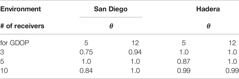
Table 4 Ratio between the coverage and the usable area, θ for the deployment of 3, 5 and 10 receivers for San Diego and the Hadera power station areas, for GDOP = 5 and GDOP = 12.

The impact of the geometrical relations between 3 receivers on the usable area, μ, and on the coverage area, C(β) , is demonstrated in Figure 7 for β = 3 and β = 4. The green, blue, and red circles are the detection areas of the green, blue, and red receivers positioned at the corresponding colored markers, respectively. Comparing Figures 7A, B, we observe that, in the latter, the receivers are located closer to each other and the size of the usable area, μ, highlighted in gray, is larger. However, the resulting coverage area, C, highlighted in light blue, for α = 5, is smaller in Figure 7D. This is due to the small distance between the receivers, which yields a smaller angle between pairs of receivers and the node to be localized, thereby leading to poor localization.

FIGURE 7

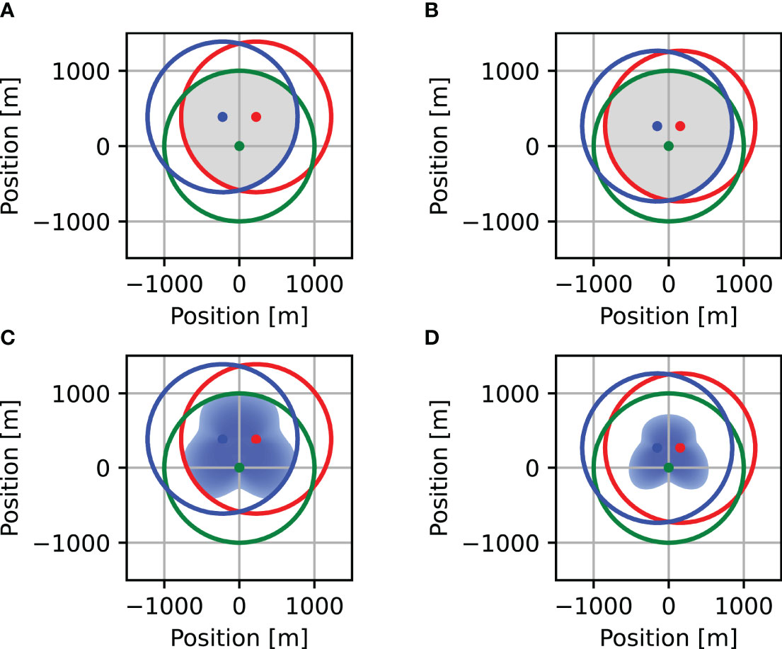
Figure 7 Effect of distance between the receivers on the usable area and the coverage area with attained positioning quality. In setup 1, plots (A, C), the receivers are placed 450m away from each other creating a usable area of S ≈ 1.782 km² and the coverage area is C ≈ 1.544 km² occupying 86% of the usable area. In setup 2, plots (B, D), the receivers are placed 300m away from each other creating a usable area of S ≈ 2.1472 km². For this setup, the receivers are closer to each other than in Setup 1, and the coverage area is C ≈ 0.791 km², occupying only 37% of the usable area. The usable area in plots (A, B) is highlighted in gray. The coverage area, plots (C, D) for GDOP ≤ 5 is highlighted in light blue.

Experiment Results

As our first performance metric, we explore the size of the usable area for CP and PDAD. Figure 8 shows the position of tags received by at least three receivers for each deployment strategy. For the sake of comparison, we also show the planned usable area and the minimum convex hull for each method. We observe that the size of the usable area obtained by PDAD is 30% larger than that produced by CP. We also observe that, in the case of CP, three of the receivers are positioned outside the usable area. This is because CP does not account for the area’s specific propagation conditions. Finally, we note that compared to the planned usable area of the CP and PDAD - marked by solid blue and green lines, respectively - the actual usable areas span to the east further than expected. This is attributed to the acoustic propagation conditions on the day of the experiment, which were likely better than those at the time of the tag’s range testing.

FIGURE 8

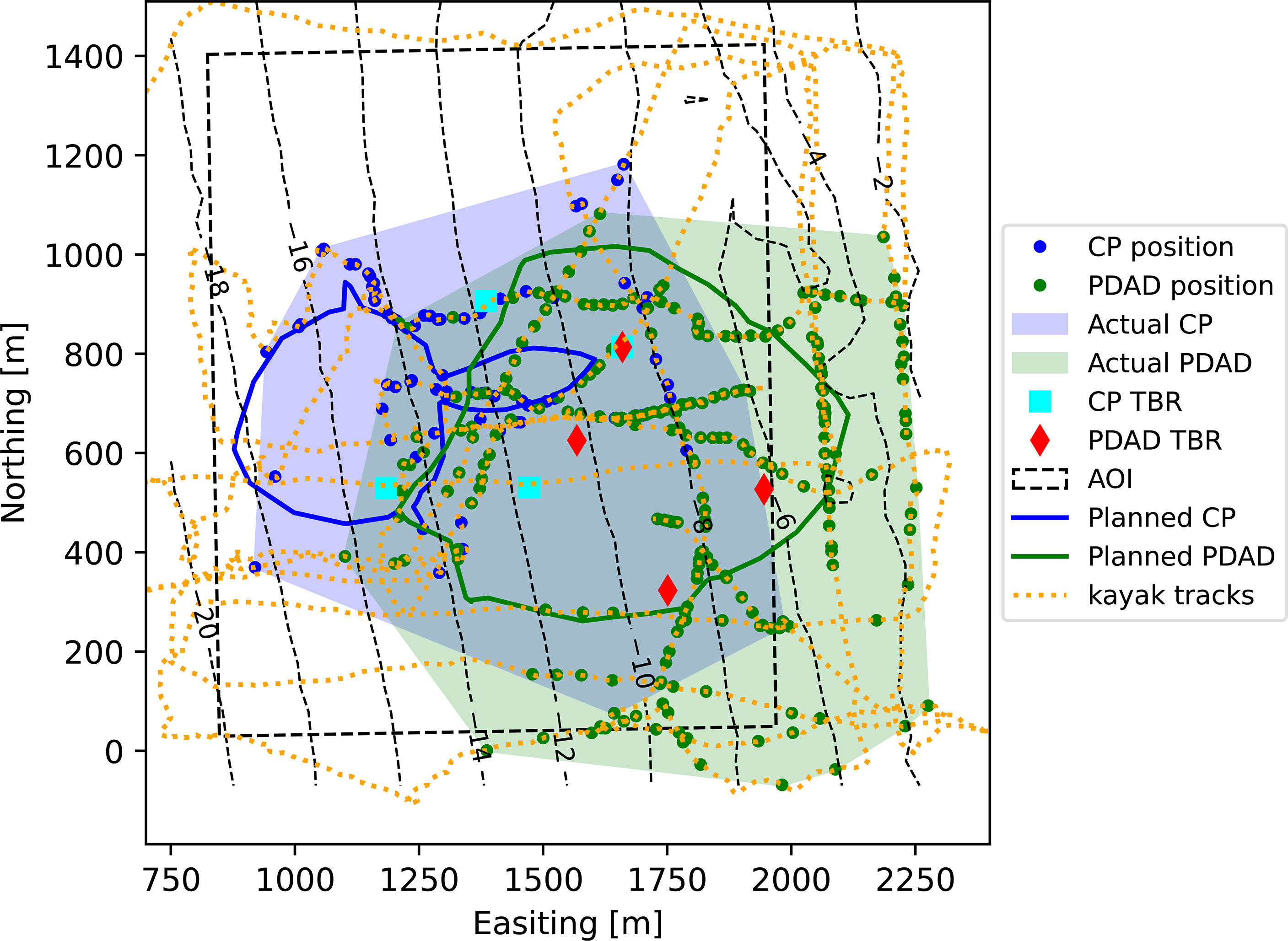
Figure 8 Positioning of tags and coverage areas for CP and PDAD methods. Light blue and green-filled areas are the minimum convex hull encompassing all points of CP and PDAD, respectively. Solid lines are the planned usable areas. Triangles are the receivers’ positions. Blue and green dots are emissions received by at least three receivers of the CP and PDAD sets, respectively.

As a second performance metric, we explored the throughput of the tags - receivers link. The results presented in Figure 9 show that the performance benefit of PDAD over CP in terms of the throughput increases with the above range. This implies that tags farther away from the receivers can still be localized by the PDAD cluster; thus, the usable PDAD area is effectively larger than that of CP. The figure also shows the throughput performance for less than three detecting receivers. While this setup does not allow localization without ambiguation, such detection indications can still provide valuable positioning information and is thus of interest (Baktoft et al., 2017). We note that, for emissions received by three or four receivers, the PDAD’s throughput is higher than that of CP by at least 80%. However, for emissions received by one or two receivers the CP throughput is sometimes higher than that of PDAD. This is because the PDAD locations are planned for localization by at least three receivers. Still, the difference is not greater than 25%, implying that the benefit of gaining larger coverage by PDAD is not highly diminished by the reduction of valuable positioning information.

FIGURE 9

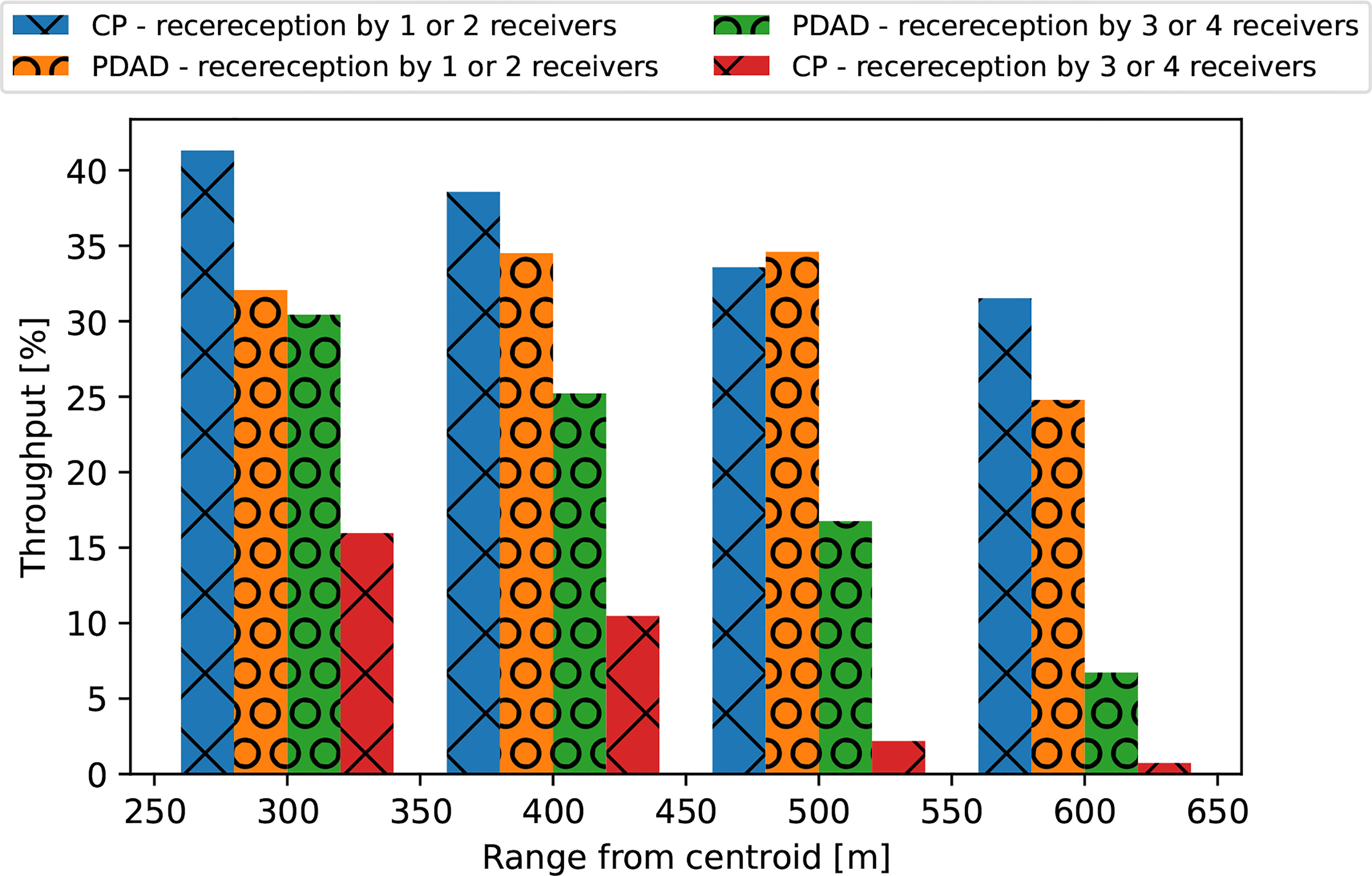
Figure 9 ξ_2,r ratio between emissions received by one or two receivers and the total number of acoustic emissions (CP - blue, PDAD - orange), and ξ_3,r - ratio between localized tags to the total number of acoustic emissions (CP - red, PDAD - green). For the PDAD method, the throughput of localized emissions is better than the CP as the range increases, i.e., more emissions are localized at larger ranges for the PDAD method, leading to a larger usable area.

In Table 5, we report the 10th, 50th and 90th percentiles of the noise measurements as obtained by each receiver. We note the relatively small noise level difference between the 10th and 90th percentiles and conclude that the detection conditions during the experiment did not vary much. From Table 5, we further note that two receivers of the PDAD cluster, namely receivers # 557 and # 558, experienced higher noise level since their position was close to the shoreline. Still, regardless the higher noise level, the PDAD outperformed CP. Finally, we observe from Figure 8 that, for PDAD, the tag’s detections are consistently along the kayak routes, whereas, for CP, the detections appear more sporadically along these tracks. This is an indication of the better stability in detection that the PDAD setup can obtain.

TABLE 5

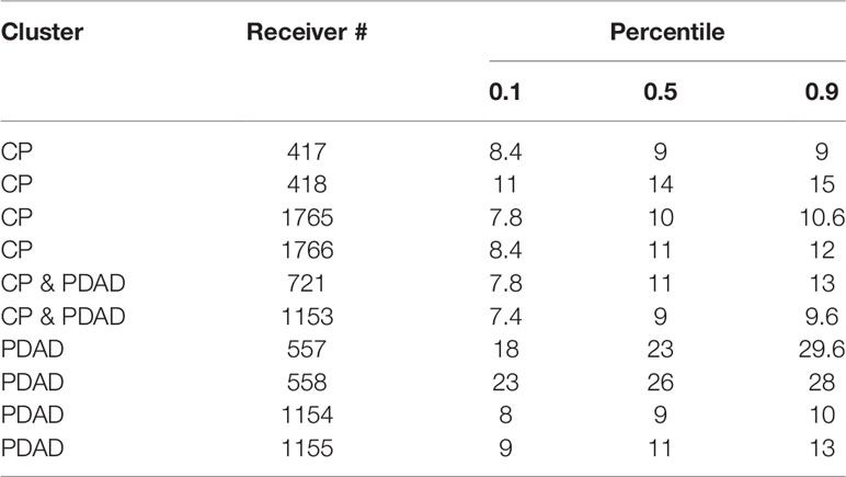
Table 5 10 Minutes average noise measured by the receivers.

Discussion

We start our discussion by surveying some relevant solutions to the deployment problem. The optimal receiver deployment problem is shown to be NP-Hard with similarities to the k-vertex problem (Tekdas and Isler, 2010; Garcia-Diaz et al., 2019). For a given graph G(V, E) and for parameters k, l, this problem seeks to discover whether G contains k vertices that cover at least one edge. Considering the high complexity required to solve the deployment problem optimally, some heuristic solutions are proposed. Much like our sub-optimal GA-based solution for PDAD, these include GA to determine the best locations for the receiving nodes (Dı́ez-González et al., 2019a; Dı́ez-González et al., 2019b), and (Díez-Gonzalez et al., 2020) by iteratively improving the position of the receivers along a given grid, while maintaining constraints in the form of clock drifts and the existence of obstacles. Due to its diversification and intensification in the search within the space of solutions, GA can also avoid falling into local minima (Mnasri et al., 2015) for diverse propagation loss conditions (Díez-González et al., 2019a). Another approach is to compute a Pareto front with a diversified local search for the optimal placement of nodes (Roa et al., 2007). Here, the deployment plan is examined under two local criteria: reception availability and quality of positioning. A different approach is simulated annealing, where a set of n nodes to be localized are randomly selected and the positions of the anchor nodes are stochastically optimized to increase the accuracy of the localization estimation (Niewiadomska-Szynkiewicz and Marks, 2009). Other heuristics are particle swarm optimization (Wang et al., 2007) and Tabu search methodologies (Laguna et al., 2009). The firefly algorithm (Tuba et al., 2018) is used to initialize anchors’ positions at the corners of the explored area, and then move them trying to increase the angle between anchors and the node to be localized, while the relative distance between the anchors and the node to be localized is decreased.

The above works obtain good results for terrestrial networks. Yet, some of the underlying assumptions may be too hard for the underwater acoustic environment. Specifically, it is assumed that the propagation loss does not change with space; that the node to be localized is either bounded inside a polygon whose anchors are its vertices or that some information about its route is known; and that a receiver can be added upon demand to increase the quality of the covered area. In our considered case, due to the spatially-dependent bathymetry, the propagation loss is often a complex location-dependent function, and the optimum coverage solution dictates positioning of receivers in non-overlapping areas.

Using the GDOP to Measure Localization

We would like to comment about our usage of the GDOP [cf. Sharp et al. (2009)] as a utility metric. We use the GDOP to assess the expected accuracy of the localization by the receivers’ deployment setup. Other common metrics are the Cramér-Rao lower bound (CRLB), which expresses a lower bound on the variance of unbiased estimators, and which is widely used as a positioning performance estimator in wireless networks (Miao et al., 2007). Alternatively, the root mean square error (RMSE) of the location estimates or the cumulative distribution probability of the location errors can both be used as a localization quality of measures (Sharp et al., 2009). However, it is useful to decouple the statistical error component of the positional error from the geometric factors of the deployment setup. We find this representation in the GDOP metric. The GDOP quantifies how errors in the ToA measurements translate into the covariance components of the estimated position, and represents the influence of the standard deviation of the measurement errors onto the solution. The GDOP values can be categorized to measure the localization quality. One such option is presented in Table 6 as proposed in (Dutt et al., 2009).

TABLE 6

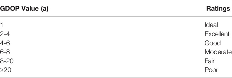
Table 6 GDOP Ratings.

Discussion of Results

We next make some comments about our results. As demonstrated in our sea experiment, optimized placement of the receivers can gain extra coverage area of about 30%. This is attributed to the high dependency of the underwater acoustic propagation on environmental conditions, such as temperature profile and the bathymetric map. This dependency is demonstrated in Figure 3, showing the different shapes of detection areas in different positions of a tag in the area of interest. This is because the propagation loss and thus the detection rate depends not only on its range from the receiver. Consequentially, there may be cases of blind spots, where, albeit short range, the tag’s emissions are not properly detected. While such a diversity may also be present in terrestrial or aerial testbeds, it is highly dominant in the underwater acoustic environment with spatial variations on the order of a few tens of meters. Hence, while our method can be applied also for other domains, it is mostly attractive for underwater testbeds. As a test case, we analyzed and tested our method with large acoustic tags, suitable for megafauna. However our method may suit smaller tags with weaker SL. Hence, by using our method, the 30% increase in the explored area holds much more impact for the task of tracking the locations of marine fauna and megafauna.

Conclusions

This study focused on developing a systematic framework for planning the deployment of underwater receivers for the task of localizing acoustically-tagged marine fauna, with test case for tracking of megafauna such as sharks, sea turtles, and seals. We formalized the deployment position as a constraint optimization problem that takes into account the environmental conditions, the desired localization quality, and a given area-of-interest that should be covered with high priority. For a flat bottom bathymetry and isothermal conditions, we showed that the common practice can achieve optimal coverage area. For the case of complex bathymetry where the complexity is too high to directly solve the problem, we offered a sub-optimal solution based on a genetic algorithm that is able to efficiently solve the problem for large areas of a few square kms and for a large number of receivers. We explored the benefits of our proposed approach in terms of the size of the coverage area and the throughput of the tags’ emissions. The performance is evaluated in numerical simulations and verified in a field experiment, using large tags suitable for tracking megafauna as a test case. The results show that the performance of our proposed deployment - in terms of the coverage area - is superior to that of the common practice. Future work will further investigate how the setup can better account for the expected seasonal changes of the SVP and verify the applicability of our method to a smaller scale testbeds, i.e. smaller tags.

Data Availability Statement

The datasets and supplementary material presented in this study can be found here: https://figshare.com/articles/dataset/Tags_emissions/17942534 (for the database - sea experiment) and https://github.com/kerentalmon/Receiver-Deployment (for the software).

Author Contributions

TA conceived and led the study. TA and RD conducted the field work. TA analyzed the data. Both authors interpreted the findings, wrote the manuscript, and RD approved the final version.

Funding

This work was supported in part by the MOST-BMBF German-Israeli Cooperation in Marine Sciences 2018-2020 (Grant # 3-16573), and by the MOST action for Agriculture, Environment, and Water for the year 2019 (Grant # 3-16728).

Conflict of Interest

The authors declare that the research was conducted in the absence of any commercial or financial relationships that could be construed as a potential conflict of interest.

Publisher’s Note

All claims expressed in this article are solely those of the authors and do not necessarily represent those of their affiliated organizations, or those of the publisher, the editors and the reviewers. Any product that may be evaluated in this article, or claim that may be made by its manufacturer, is not guaranteed or endorsed by the publisher.

Footnotes

1. ^ note that when the source is mobile β = 2 will also support 2D localization as shown in (Alexandri et al., 2018).

References

Alexandri T., Diamant R. (2022). Receiver Deployment Experiment Data Set. doi: 10.6084/m9.figshare.17942534.v4

CrossRef Full Text | Google Scholar

Alexandri T., Miller E., Spanier E., Diamant R. (2018). Tracking the Slipper Lobster Using Acoustic Tagging: Testbed Description. IEEE J. Ocean. Eng. 45, 577–585. doi: 10.1109/JOE.2018.2880862

CrossRef Full Text | Google Scholar

Alexandri T., Shamir Z. Z., Bigal E., Scheinin A., Tchernov D., Diamant R. (2019). Localization of Acoustically Tagged Marine Animals in Under-Ranked Conditions. IEEE Trans. Mobile. Comput. 20, 1126–1137. doi: 10.1109/TMC.2019.2959765

CrossRef Full Text | Google Scholar

Ankenbrandt C. A. (1991). An Extension to the Theory of Convergence and a Proof of the Time Complexity of Genetic Algorithms. In. Found. Genet. Algorithm. (Elsevier). 1, 53–68. doi: 10.1016/B978-0-08-050684-5.50007-0

CrossRef Full Text | Google Scholar

Bahrami N., Khamis N. H. H., Baharom A., Yahya A. (2016). Underwater Channel Characterization to Design Wireless Sensor Network by Bellhop. Telkomnika 14, 110. doi: 10.12928/telkomnika.v14i1.2454

CrossRef Full Text | Google Scholar

Baktoft H., Gjelland K.Ø., Økland F., Thygesen U. H. (2017). Positioning of Aquatic Animals Based on Time-of-Arrival and Random Walk Models Using Yaps (Yet Another Positioning Solver). Sci. Rep. 7, 1–10. doi: 10.1038/s41598-017-14278-z

PubMed Abstract | CrossRef Full Text | Google Scholar

Berejikian B., Moore M., Jeffries S. J. (2016). Predator-Prey Interactions Between Harbor Seals and Migrating Steelhead Trout Smolts Revealed by Acoustic Telemetry. Mar. Ecol. Prog. Ser. 543, 21–35. doi: 10.3354/meps11579

CrossRef Full Text | Google Scholar

Blum A., Dan C., Seddighin S. (2021). Learning Complexity of Simulated Annealing. In. Int. Conf. Artif. Intell. Stat (PMLR). 130, 1540–1548.

Google Scholar

Clausen J. (1999). Branch and Bound Algorithms-Principles and Examples (Copenhagen, Denmark: Department of Computer Science, University of Copenhagen), 1–30.

Google Scholar

Corus D., Dang D.-C., Eremeev A. V., Lehre P. K. (2017). Level-Based Analysis of Genetic Algorithms and Other Search Processes. IEEE Trans. Evolution. Comput. 22, 707–719. doi: 10.1109/TEVC.2017.2753538

CrossRef Full Text | Google Scholar

Diamant R., Kipnis D., Bigal E., Scheinin A., Tchernov D., Pinchasi A. (2019). An Active Acoustic Track-Before-Detect Approach for Finding Underwater Mobile Targets. IEEE J. Select. Top. Signal Process. 13, 104–119. doi: 10.1109/JSTSP.2019.2899237

CrossRef Full Text | Google Scholar

Díez-González J., Álvarez R., González-Bárcena D., Sánchez-González L., Castejón-Limas M., Perez H. (2019a). Genetic Algorithm Approach to the 3d Node Localization in Tdoa Systems. Sensors 19, 3880. doi: 10.3390/s19183880

CrossRef Full Text | Google Scholar

Díez-Gonzalez J., Álvarez R., Perez H. (2020). Optimized Cost-Effective Node Deployments in Asynchronous Time Local Positioning Systems. IEEE Access 8, 154671–154682. doi: 10.1109/ACCESS.2020.3018624

CrossRef Full Text | Google Scholar

Díez-González J., Álvarez R., Sánchez-González L., Fernández-Robles L., Pérez H., Castejón-Limas M. (2019b). 3d TDOA Problem Solution With Four Receiving Nodes. Sensors 19, 2892. doi: 10.3390/s19132892

CrossRef Full Text | Google Scholar

Divins D., Metzger D. (2021) NGDC Coastal Relief Model. Download Provided by the Southern California Coastal Ocean Observing System. Available at: http://www.ngdc.noaa.gov/mgg/coastal/coastal.html.

Google Scholar

Dubrovinskaya E., Diamant R., Casari P. (2017). “Anchorless Underwater Acoustic Localization,” in . In 2017 14th Workshop on Positioning, Navigation and Communications (WPNC) (Bremen, Germany: IEEE), 1–6.

Google Scholar

Dutt V. S. I., Rao G. S. B., Rani S. S., Babu S. R., Goswami R., Kumari C. U. (2009). Investigation of GDOP for Precise User Position Computation With All Satellites in View and Optimum Four Satellite Configurations. J. Ind. Geophys. Union. 13, 139–148.

Google Scholar

Fewell M. P. (2006). “Area of Common Overlap of Three Circles,” in Tech. Rep. DSTO-TN-0722, (Edinburgh, Australia: Defence Science and Technology Organisation Edinburgh (Australia) Maritime).

Google Scholar

Florko K. R., Davidson E. R., Lees K. J., Hammer L. J., Lavoie M.-F., Lennox R. J., et al. (2021). Tracking Movements of Decapod Crustaceans: A Review of a Half-Century of Telemetry-Based Studies. Mar. Ecol. Prog. Ser. 679, 219–239. doi: 10.3354/meps13904

CrossRef Full Text | Google Scholar

Garcia-Diaz J., Menchaca-Mendez R., Menchaca-Mendez R., Hernández S. P., Pérez-Sansalvador J. C., Lakouari N. (2019). Approximation Algorithms for the Vertex K-Center Problem: Survey and Experimental Evaluation. IEEE Access 7, 109228–109245. doi: 10.1109/ACCESS.2019.2933875

CrossRef Full Text | Google Scholar

Gazit T., Apostle R., Branton R. (2013). Deployment, Tracking, and Data Management: Technology and Science for a Global Ocean Tracking Network. J. Int. Wildlife. Law Policy 16, 112–127. doi: 10.1080/13880292.2013.805058

CrossRef Full Text | Google Scholar

Gul S., Zaidi S. S. H., Khan R., Wala A. B. (2017). “Underwater Acoustic Channel Modeling Using Bellhop Ray Tracing Method,” in In 2017 14th International Bhurban Conference on Applied Sciences and Technology (IBCAST) (Bhurban, Pakistan: IEEE), 665–670.

Google Scholar

Hockersmith E. E., Beeman J. W. (2012). A History of Telemetry in Fishery Research. Telemetry. Technique.: User. Guide. Fish. Res. 542, 7–19. doi: 10.1080/03632415.2014.903840

CrossRef Full Text | Google Scholar

Huveneers C., Simpfendorfer C. A., Kim S., Semmens J. M., Hobday A. J., Pederson H., et al. (2016). The Influence of Environmental Parameters on the Performance and Detection Range of Acoustic Receivers. Methods Ecol. Evol. 7, 825–835. doi: 10.1111/2041-210X.12520

CrossRef Full Text | Google Scholar

Jackson G. D. (2011). The Development of the Pacific Ocean Shelf Tracking Project Within the Decade Long Census of Marine Life. PloS One 6, e18999. doi: 10.1371/journal.pone.0018999

PubMed Abstract | CrossRef Full Text | Google Scholar

Kaplan E., Hegarty C. (2005). “Performance of Stand-Alone Gnss,” in Understanding GPS: Principles and Applications (Boston, MA, USA: Artech House), 661–678.

Google Scholar

Kessel S., Cooke S., Heupel M. R., Hussey N., Simpfendorfer C., Vagle S., et al. (2014). A Review of Detection Range Testing in Aquatic Passive Acoustic Telemetry Studies. Rev. Fish. Biol. Fish. 24, 199–218. doi: 10.1007/s11160-013-9328-4

CrossRef Full Text | Google Scholar

Kraus R. T., Holbrook C. M., Vandergoot C. S., Stewart T. R., Faust M. D., Watkinson D. A., et al. (2018). Evaluation of Acoustic Telemetry Grids for Determining Aquatic Animal Movement and Survival. Methods Ecol. Evol. 9, 1489–1502. doi: 10.1111/2041-210X.12996

CrossRef Full Text | Google Scholar

Laguna M., Roa J. O., Jiménez A. R., Seco F. (2009). Diversified Local Search for the Optimal Layout of Beacons in an Indoor Positioning System. IIE. Trans. 41, 247–259. doi: 10.1080/07408170802369383

CrossRef Full Text | Google Scholar

Lea J. S., Humphries N. E., von Brandis R. G., Clarke C. R., Sims D. W. (2016). Acoustic Telemetry and Network Analysis Reveal the Space Use of Multiple Reef Predators and Enhance Marine Protected Area Design. Proc. R. Soc. B.: Biol. Sci. 283, 20160717.

Google Scholar

Lee D., Lin A. (1986). Computational Complexity of Art Gallery Problems. IEEE Trans. Inf. Theory 32, 276–282. doi: 10.1109/TIT.1986.1057165

CrossRef Full Text | Google Scholar

Lennox R. J., Nilsen C. I., Nash A., Hanssen E. M., Johannesen H. L., Berhe S., et al. (2021). Laboratory and Field Experimental Validation of Two Different Predation Sensors for Instrumenting Acoustic Transmitters in Fisheries Research. Fisheries 46, 565–573. doi: 10.1002/fsh.10669

CrossRef Full Text | Google Scholar

Miao H., Yu K., Juntti M. J. (2007). Positioning for Nlos Propagation: Algorithm Derivations and Cramer–Rao Bounds. IEEE Trans. Vehicul. Technol. 56, 2568–2580. doi: 10.1109/TVT.2007.899948

CrossRef Full Text | Google Scholar

Mnasri S., Thaljaoui A., Nasri N., Val T. (2015). “A Genetic Algorithm-Based Approach to Optimize the Coverage and the Localization in the Wireless Audio-Sensors Networks,” in In 2015 International Symposium on Networks, Computers and Communications (ISNCC) (Yasmine Hammamet, Tunisia: IEEE), 1–6.

Google Scholar

National Research Council (2003). Ocean Noise and Marine Mammals (Washington, DC: The National Academies Press). doi: 10.17226/10564

CrossRef Full Text | Google Scholar

Niewiadomska-Szynkiewicz E., Marks M. (2009). Optimization Schemes for Wireless Sensor Network Localization. Int. J. Appl. Math. Comput. Sci. 19, 291–302. doi: 10.2478/v10006-009-0025-3

CrossRef Full Text | Google Scholar

Pickholtz R. S., Kiflawi M., Friedlander A. M., Belmaker J. (2018). Habitat Utilization by an Invasive Herbivorous Fish (Siganus Rivulatus) in its Native and Invaded Range. Biol. Invas. 20, 3499–3512. doi: 10.1007/s10530-018-1790-4

CrossRef Full Text | Google Scholar

Porter M. B. (2011). The Bellhop Manual and User’s Guide: Preliminary Draft Vol. 260 (La Jolla, CA, USA, Tech. Rep: Heat, Light, and Sound Research, Inc.).

Google Scholar

Rajagopal N., Chayapathy S., Sinopoli B., Rowe A. (2016). “Beacon Placement for Range-Based Indoor Localization,” in In 2016 International Conference on Indoor Positioning and Indoor Navigation (IPIN) (Alcalá de Henares, Spain: IEEE), 1–8.

Google Scholar

Reubens J., Aarestrup K., Meyer C., Moore A., Okland F., Afonso P. (2021). Compatibility in Acoustic Telemetry. Anim. Biotelemet. 9, 1–6. doi: 10.1186/s40317-021-00253-z

CrossRef Full Text | Google Scholar

Roa J. O., Jiménez A. R., Seco F., Prieto J. C., Ealo J. (2007). “Optimal Placement of Sensors for Trilateration: Regular Lattices vs Meta-Heuristic Solutions,” in In International Conference on Computer Aided Systems Theory (Las Palmas de Gran Canaria, Spain: Springer), 780–787.

Google Scholar

Rylander B. I. (2001). Computational Complexity and the Genetic Algorithm (University of Idaho).

Google Scholar

Salon S., Crise A., Picco P., De Marinis E., Gasparini O. (2003). “Sound Speed in the Mediterranean Sea: An Analysis From a Climatological Data Set,” in In Annales Geophysicae, vol. 21. (Göttingen, Germany: Copernicus GmbH), 833–846.

Google Scholar

Shabi J., Reich Y., Diamant R. (2017). Planning the Verification, Validation, and Testing Process: A Case Study Demonstrating a Decision Support Model. J. Eng. Des. 28, 171–204. doi: 10.1080/09544828.2016.1274964

CrossRef Full Text | Google Scholar

Sharp I., Yu K., Guo Y. J. (2009). GDOP Analysis for Positioning System Design. IEEE Trans. Vehicul. Technol. 58, 3371–3382. doi: 10.1109/TVT.2009.2017270

CrossRef Full Text | Google Scholar

Shiu L. C., Lee C. Y., Yang C. S. (2010). The Divide-and-Conquer Deployment Algorithm Based on Triangles for Wireless Sensor Networks. IEEE Sens. J. 11, 781–790. doi: 10.1109/JSEN.2010.2059006

CrossRef Full Text | Google Scholar

Tekdas O., Isler V. (2010). Sensor Placement for Triangulation-Based Localization. IEEE Trans. Automat. Sci. Eng. 7, 681–685. doi: 10.1109/TASE.2009.2037135

CrossRef Full Text | Google Scholar

Thelma Biotel (2021) Pinpoint Positioning System. Guidelines Provided by Thelma Biotel. Available at: https://www.thelmabiotel.com/service/pinpoint/.

Google Scholar

Thums M., Whiting S. D., Reisser J. W., Pendoley K. L., Pattiaratchi C. B., Harcourt R. G., et al. (2013). Tracking Sea Turtle Hatchlings—a Pilot Study Using Acoustic Telemetry. J. Exp. Mar. Biol. Ecol. 440, 156–163. doi: 10.1016/j.jembe.2012.12.006

CrossRef Full Text | Google Scholar

Tuba E., Tuba M., Beko M. (2018). “Two Stage Wireless Sensor Node Localization Using Firefly Algorithm,” in In Smart Trends in Systems, Security and Sustainability (Singapore: Springer), 113–120.

Google Scholar

Urick R. J. (1983). “Propagation of Sound in the Sea: Transmission Loss I,” in Principles of Underwater Sound (New York, NY (USA: McGraw-Hill Book), 99–143.

Google Scholar

Wang X., Ma J.-J., Wang S., Bi D.-W. (2007). Distributed Particle Swarm Optimization and Simulated Annealing for Energy-Efficient Coverage in Wireless Sensor Networks. Sensors 7, 628–648. doi: 10.3390/s7050628

CrossRef Full Text | Google Scholar

Yarlagadda R., Ali I., Al-Dhahir N., Hershey J. (2000). Gps. Gdop. Metric. IEE. Proceedings-radar. Sonar. Navigat. (IET) 147, 259–264. doi: 10.1049/ip-rsn:20000554

CrossRef Full Text | Google Scholar

Zhang W., Korf R. E. (1992). “An Average-Case Analysis of Branch-and-Bound With Applications: Summary of Results. San Jose, California, USA: AAAI, 545–550.

Google Scholar

Appendix

An interesting case to explore is the deployment of 3 receivers on a flat seabed with isotropic propagation loss and with no constraint on the area of interest. The question explored is: What is the best receivers setup to attain the maximal covered area C. The expected answer is an equilateral triangle setup (Fewell, 2006; Shiu et al., 2010). Yet, the proof is not trivial.

Let R be the receiving radius of a receiver of all 3 receivers, and let l be the range between the 3 receivers deployed in an equilateral setup. Without the loss of generality, let the position of one of the receivers be at x₂,y₂ = (0,0). Consider the setup $x_1,y_1=\left(0.5l,0.5\sqrt{3}l\right)$, $x_3,y_3=\left(-0.5l,0.5\sqrt{3}l\right)$. For l = 0, the 3 receivers are placed in the same location and S = πR² .We derive the area of S for any $0\le l\le \sqrt{3}R$. Figure 10 illustrates this setup.

FIGURE 10

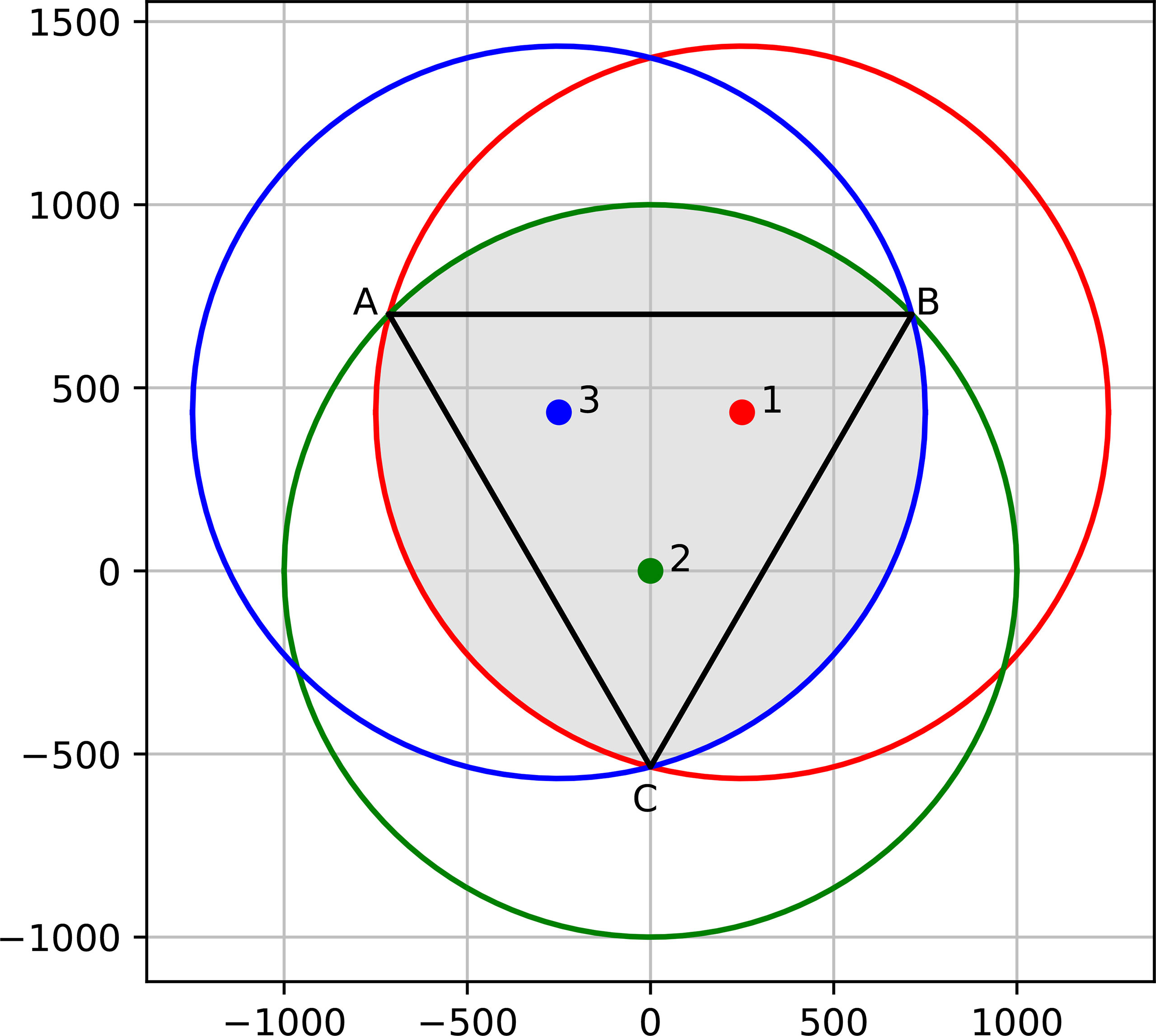
Figure 10 The receivers’ position are marked by numbers; the intersections between the contour of the receiving ranges are marked by letters. The shaded area is the usable receiving area S. The distance between the 3 receivers is 0 ≤ x ≤ R.

Referring to Figure 10, the total usable area S = S_T + 3S_S, where S_T denotes the area of triangle ABC and S_S denotes the segments area between the cords AB, BC, CA. The intersection points of the two circles ${\left(x-a_1\right)}^2+{\left(y-b_1\right)}^2=R_1^2$ and ${\left(x-a_2\right)}^2+{\left(y-b_2\right)}^2=R_2^2$ are

$\begin{array}{ll}\begin{array}{l}{x}_{1,2}=\frac{a_1+a_2}{2}+\frac{\left(a_2-a_1\right)\left(R_1^2-R_2^2\right)}{2*l^2}\pm 2\frac{b_1-b_2}{l^2}d\hfill \\ y_{1,2}=\frac{b_1+b_2}{2}+\frac{\left(b_2-b_1\right)\left(R_1^2-R_2^2\right)}{2*l^2}\mp 2\frac{a_1-a_2}{l^2}d\hfill \end{array}& (19)\end{array}$

where

$\begin{array}{ll}d=0.25\sqrt{\left(l+R_1+R_2\right)\left(l+R_1-R_2\right)\left(l-R_1+R_2\right)\left(-l+R_1+R_2\right)}.& (20)\end{array}$

For the case at hand, R₁ = R₂ = R such that the distance between any two intersection points creating triangle ABC is $D=0.5\left(\sqrt{3\left(4R^2-l^2\right)}-l\right)$. Thus,

$\begin{array}{ll}{S}_{\text{S}}=R^2{\text{sin}}^{-1}\begin{array}{l}{S}_{\text{T}}=0.25\sqrt{3}{D}^2\left(28\right)\hfill \\ \left(\frac{D}{2R}\right)-0.25D\sqrt{4R^2-D^2}\hfill \\ S=S_{\text{T}}+3S_{\text{S}}\hfill \end{array}& (21)\end{array}$

Figure 4 shows the coverage area for the distance between the receivers of $0\le l\le \sqrt{3}R$ for a number of GDOP values.l