Air-Sea Latent Heat Flux Anomalies Induced by Oceanic Submesoscale Processes: An Observational Case Study

The classical theory predicts that a geostrophically balanced mesoscale eddy can cause a sea surface temperature (SST) anomaly related to Ekman pumping. Previous studies show that an eddy-induced SST anomaly can result in a sea surface latent heat flux (LH) anomaly at a maximum magnitude of ∼O(10) Wm^–2, decaying radially outward from the center to the margin. In this study, we investigate the LH anomalies associated with submesoscale processes within a cyclonic eddy for the first time using recent satellite-ship-coordinated air-sea observations in the South China Sea. Unbalanced submesoscale features can be identified as submesoscale SST fronts. Along the ship track, the SST strikingly decreases by 0.5°C within a horizontal distance of ∼1.5 km and increases quickly by 0.9°C with a spatial interval of ∼3.6 km. The along-track SST is decomposed into three parts: large-scale south-north fronts and anomalies induced by mesoscale and submesoscale motions. Our analysis shows that the amplitude of the LH anomaly induced by the mesoscale SST anomaly is 12.3 Wm^–2, while it is 14.3 Wm^–2 by unbalanced submesoscale motions. The mean (maximum) spatial gradient of the submesoscale LH anomalies is 1.7 (75.7) Wm^–2km^–1, which is approximately 1.5 times those (1.2 and 59.9 Wm^–2km^–1) in association with mesoscale eddies. The spectra of LH and SST anomalies show similar peaks at ∼15 km before sloping down with a power law between k^–2 and k^–3, indicating the underlying relationship between the LH variance and submesoscale processes.

Introduction

The air-sea latent heat flux (LH) is closely associated with sea surface evaporation (E), with a relation of Q_LH = ρ_wL_eE between them (Yu, 2007), where ρ_w is the density of seawater and L_e is the coefficient for the latent heat of vaporization. The LH undoubtedly involves every air-sea interaction process, with water vapor leaving the sea surface and the release of heat after condensation. The LH can be initially estimated by the Reynolds stress $\overline{{\mathit{\text{w}}}^{\prime }{\mathit{\text{q}}}^{\prime }}$ at the marine atmospheric boundary layer (MABL), where w′ and q′ are the fluctuations of atmospheric vertical velocity and specific humidity, respectively. However, the variables of w′ and q′ are difficult to observe. Following the Monin-Obukhov similarity theory (Monin and Obukhov, 1954), the LH is conventionally computed using air-sea variables in bulk formulas (Liu et al., 1979; Fairall et al., 2003; Edson et al., 2013):

${\mathit{\text{Q}}}_{\mathit{LH}}={\mathbf{\rho }}_{\mathit{a}}{\mathit{\text{L}}}_{\mathit{e}}{\mathit{\text{c}}}_{\mathit{E}}\left|\overrightarrow{{\mathit{\text{u}}}_{\mathit{z}}}\right|\left({\mathit{\text{q}}}_{\mathit{s}}-{\mathit{\text{q}}}_{\mathit{a}}\right)(1)$

where ρ_a is the air density, c_E is the turbulent exchange coefficient, $\left|\overline{{\mathit{\text{u}}}_{\mathit{z}}}\right|$ is the wind speed, and δq = q_s − q_a represents the air-sea specific humidity difference.

The LH plays a vital role in redistributing the sea surface heat over the global oceans; the LH balances the majority of the incoming solar radiation to help achieve a global sea surface heat budget balance (Cayan, 1992; Carton and Zhou, 1997; Foltz and McPhaden, 2005; Trenberth et al., 2009; Yu, 2019). Its variation is a reflection of coupled air-sea interactions. For example, basin-scale variations in the LH and analogically air-sea sensible heat flux (SH) can be determined by anomalies in the wind speed and air-sea thermal effects induced by large-scale atmospheric and oceanic oscillations (Cayan, 1992; Yu, 2007; Song and Yu, 2012). An extreme LH accompanies enhanced wind speed and air-sea humidity differences during tropical cyclones (TCs, Song et al., 2021), which can contribute to maintaining a cold wave and potential feedback to the intensity of the TCs (Lin et al., 2009). High-resolution buoy observations are used to investigate the diurnal variations in the LH over western boundary current systems (Clayson and Edson, 2019), equatorial oceans (Yan et al., 2021) and even coastal seas (Song, 2020), with amplitudes ranging from approximately 10 to 50 Wm^–2. The roles of the wind speed ($\left|\overline{{\mathit{\text{u}}}_{\mathit{z}}}\right|$) and air-sea humidity difference (δq = q_s − q_a) in contributing to the diurnal variations in the LH depend on the stability of the MABL. Wind (humidity difference) tends to play a predominant role in determining the LH variations under a stable (unstable) MABL.

Ocean dynamics can also modulate the sea surface temperature (SST) and LH, as the near-surface specific humidity is largely determined by a saturated SST in terms of the Tetens empirical relation (Murray, 1986). The basin-scale SST anomalies are partially governed by Ekman transport in response to atmospheric oscillations in the North Atlantic (Marshall et al., 2001; Visbeck et al., 2003; Hurrell and Deser, 2009) or Southern Ocean (Hall and Visbeck, 2002; Oke and England, 2004; Ito et al., 2010), which gives rise to anomalies in the LH. As the largest reservoir for global oceanic kinetic energy (Ferrari and Wunsch, 2009), mesoscale eddies lead to significant anomalies in the sea surface height (SSH, Chelton et al., 2011) and SST (Chelton and Xie, 2010; Hausmann and Czaja, 2012; Frenger et al., 2013), with typical horizontal scales of 50–300 km and time scales ranging from weeks to months. The composite analysis of the SSH and LH in the South Atlantic (the Brazil-Malvinas confluence and the Agulhas Current Retroflection, Villas Bôas et al., 2015) and northern South China Sea (SCS, Liu et al., 2020) demonstrates that the magnitudes of LH anomalies induced by mesoscale eddies are ∼O(10) Wm^–2, which reveals a quasi-circular imprinted pattern within the eddy interior that decays radially outward from the center to the margin. These regional estimates basically answer how mesoscale eddies affect LH anomalies quantitatively using eddy-resolving datasets, which provide insight into air-sea interactions over mesoscale eddies.

However, recent studies have shown that submesoscale flows with large Rossby numbers of ∼O(1) are also omnipresent in the ocean (McWilliams, 2016). They are characterized by a variety of small-scale filaments and vortices with a horizontal scale of ∼O(10) km and a time scale of ∼O(1) day. Observations of submesoscale processes are challenging because these small-scale events are always intermittent and evolving rapidly. Great efforts have been made to investigate the dynamics of submesoscale turbulence based on in situ observations (Thomas et al., 2016; Thompson et al., 2016; Yu et al., 2019; Siegelman et al., 2020; etc.). A recent study shows that the vertical heat flux is estimated to be as high as ∼2,000 Wm^–2 in the upper ocean, which is mostly attributed to strain-induced submesoscale activities (Siegelman et al., 2020). Strong temperature fronts in the mixed layer associated with instabilities can also modify the SST and air-sea heat fluxes. However, less attention has been given to the air-sea turbulent heat flux anomalies in response to these submesoscale motions, with additional observation requirements of meteorological variables in the MABL. One scientific question may arise: how many LH anomalies can be generated by submesoscale motions compared with those induced by mesoscale eddies at a magnitude of O(10) Wm^–2? To answer this question, an in situ observational experiment is designed and conducted across the center of a cyclonic eddy in the central SCS. The following sections demonstrate the measurements and findings. The air-sea sensible heat flux is not studied in this study, as it is quite low in the boreal warm season with a smaller air-sea temperature difference.

Materials and Methods

Observations

High-Resolution Ship-Borne Air-Sea Measurements

Air-sea heat fluxes are observed during the mesoscale eddy cruise in the SCS from May 6–7, 2021 (Song et al., 2022, submitted to JGR: Oceans, attached). The SST is observed at a depth of 5 m using SBE21 SeaCAT Thermosalinography,¹ which mounts near the seawater intake of R/V TAN KAH KEE. Across the eddy center (Figure 1) at approximately 115.9°E, 17.3°N, the SST is recorded every 10 min with a spatial interval of approximately 50 m at a vessel velocity of ∼10 knots. A Vaisala AWS430 automatic weather station² is anchored to the front deck. The meteorological sensor for air humidity and temperature is an HMP155 model, and the sensors are WMT700 and BARO-1 models for wind and pressure observations. The observational height for humidity, air temperature and atmospheric pressure is approximately 13.5 m, while it is 14.5 m for the wind speed and direction measurements. In terms of the logarithmic relation for meteorological variables in the MABL (e.g., Large and Pond, 1981; Smith, 1988), the value is adjusted to 10 m and corrected for atmospheric stability using Monin-Obukhov similarity theory (e.g., Fairall et al., 2003). The meteorological parameters are averaged every minute with a spatial interval of approximately 300 m. The vertical profile of meteorological variables is observed by the sounding balloons every 6 h along the ship track (Figure 1). Two profiles are obtained within the cyclonic eddy, and two are out of the margins. All these air-sea observations across the eddy are conducted within 1 day from early morning to the evening at a high spatial resolution, providing the opportunity to investigate the LH anomalies induced by the meso- and submesoscale processes.

FIGURE 1

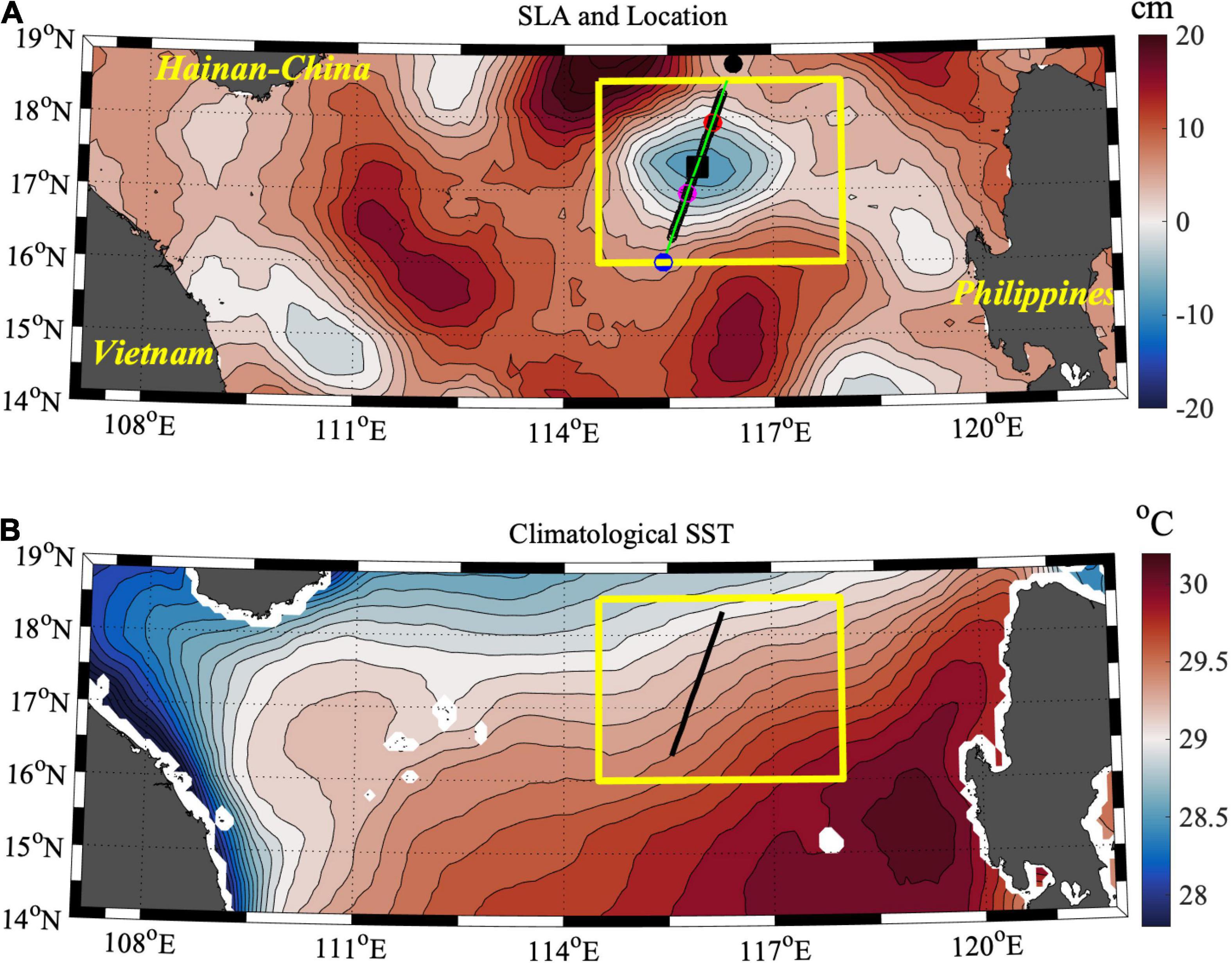
Figure 1. (A) Two-day (May 6 and 7, 2021) mean sea level anomaly (SLA, unit: cm) in the central SCS with a contour interval of 2 cm. The SLAs in the yellow frame highlight the specific cyclonic eddy in this study, and the green line across the center of the eddy indicates the cross-section of the ship-borne air-sea measurements. The black square indicates the eddy center (115.9°E, 17.3°N) with the maximum negative SLA. The colored dots along the track indicate the sounding balloon observations to obtain the vertical profile of meteorological variables at the standard times of UT050617 (LT050701, black dot), UT050623 (LT050707, red dot), UT050705 (LT050713, magenta dot) and UT050711 (LT050719, blue dot). The dynamics of the stimulated imbalance inside the cyclonic eddy are investigated using MVP 300 observations (black circles) in another study (Song et al., 2022). (B) Nineteen-year climatological MWIR SST in May from 2003 to 2021.

High-Resolution Satellite Achievements

In situ ship-borne measurements are coordinated with near-real-time satellite altimeter observations to investigate the LH anomalies associated with submesoscale motions in the central SCS. Sea level anomaly (SLA) data with a high spatial resolution of (1/8)° × (1/8)° are obtained based on the commercial contract between the State Oceanic Administration (SOA) and Archiving, Validation, and Interpretation of Satellite Oceanographic data (AVISO). The daily 9 km gridded SST maps during the observation period from the remote sensing system (REMSS) are used as a reference for ship-borne observations. The latest version (5th) of this SST product integrates global microwave imager (GMI) (microwave) and Visible Infrared Imaging Radiometer Suite-National Polar-Orbiting Partnership (VIIRS-NPP) (infrared) measurements; this version also combines the through-cloud capabilities of the microwave data with the high spatial resolution and near-coastal capability of the infrared SST data, hereafter the MWIR SST. Figure 1B shows the nineteen-year (2003–2021) climatological mean SST in May, indicating large-scale south-north fronts in association with ocean dynamics and air-sea interactions (e.g., Qu, 2001). To avoid the effects of long-term climate mode (e.g., El Niño; Wang et al., 2006), the satellite-based south-north SST fronts are obtained by averaging the daily observations over 10 days before and after the cross-sectional ship observations. The two-dimensional SST data are linearly interpolated to calculate a satellite-based SST along the ship track. This is an important reference for ship-borne observations to understand the large-scale background SST fronts.

Latent Heat Flux Estimates via the Bulk Algorithm

Decomposition of Sea Surface Temperature Anomalies Associated With Multiscale Dynamics

The SST anomalies associated with different dynamic processes are decomposed by the following relation:

$\begin{array}{c}{\mathbf{\theta }}^{\prime }=\mathbf{\theta }-\overline{\mathbf{\theta }}-{\mathbf{\theta }}_{\mathit{linear}}=\overbrace{{(\mathbf{\theta }-\overline{\mathbf{\theta }}-{\mathbf{\theta }}_{\mathit{linear}})}_{\mathit{rm}}}\hfill \\ +\underbrace{[(\mathbf{\theta }-\overline{\mathbf{\theta }}-{\mathbf{\theta }}_{\mathit{linear}})-{(\mathbf{\theta }-\overline{\mathbf{\theta }}-{\mathbf{\theta }}_{\mathit{linear}})}_{\mathit{rm}}}]\hfill \end{array}(2)$

where θ represents the SST or another arbitrary variable used in another study (Barkan et al., 2017); the overbar denotes the cross-sectional mean magnitude of the variable, θ_linear represents the linear large-scale south-north SST fronts (Figure 1B) and the prime indicates the anomaly with respect to the mean state. The subscript rm indicates a 30 km running mean to obtain the signal of mesoscale eddy ${\mathbf{\theta }}_{\mathit{meso}}={(\mathbf{\theta }-\overline{\mathbf{\theta }}-{\mathbf{\theta }}_{\mathit{linear}})}_{\mathit{rm}}$. The radius of the cyclonic eddy in this study is approximately 90 km (local first baroclinic Rossby radius of deformation ∼55 km, Chelton et al., 1998), which is simply obtained as a geometrical feature (Chelton et al., 2011) measured from the center with the maximal negative SLA to the enclosed zero contour. The 30 km spatial running mean is equivalent to a filter operator to decompose the mean and the perturbation, as used in Barkan et al. (2017). This method is also similar to spatially high-pass filtering with half-power filter cutoffs in space (Chelton et al., 2011). The SST anomalies associated with the submesoscale motions can be extracted by removing the running mean results: ${\mathbf{\theta }}_{\mathit{submeso}}=(\mathbf{\theta }-\overline{\mathbf{\theta }}-{\mathbf{\theta }}_{\mathit{linear}})-{(\mathbf{\theta }-\overline{\mathbf{\theta }}-{\mathbf{\theta }}_{\mathit{linear}})}_{\mathit{rm}}$. The mesoscale signal can be linearly obtained based on Eq. (2). However, the non-linearity of mesoscale eddies would cause some uncertainty in the definition of “submesoscale.” For example, SST signals due to non-linear mesoscale straining advection may be classified into submesoscale signals. We admit that the interference factor of non-linearity does exist in this analysis. It is assumed that the smaller uncertainty does not affect the quantitative estimates of the LH anomalies induced by meso- and submesoscale processes.

Figure 2A shows satellite and shipboard observations of the SST and its linear south-north front. The ship-borne raw SST indicates an increase from north to south due to latitudinal solar radiation. However, a striking decrease in the SST occurs along the southern margin of the eddy. The SST decreases by 0.5°C within a horizontal distance of ∼1.5 km and increases by 0.9°C with a spatial interval of ∼3.6 km (highlighted in Figure 3), which indicates a strong front and instability. The same large-scale linear front is found with a magnitude of 0.24°C per 100 km based on satellite observations. By removing the south-north SST front, the SST anomalies induced by mesoscale and submesoscale motions can be decomposed based on Eq. (2), where the latter is known to be geostrophically unbalanced. There appears evident SST cooling with a maximum (mean) magnitude of −0.1 (0.05)°C around the eddy center (Figure 2B) in terms of eddy-induced Ekman pumping (Falkowski et al., 1991; Gaube et al., 2015). However, the strength of SST cooling is smaller than the subsurface temperature anomalies beneath the mixed layer, possibly due to the air-sea damping effect at the sea surface. The SST anomalies as a proxy for submesoscale dynamics present dramatic submesoscale variability across the cyclonic eddy. The alternations range from an extremely negative value to a positive value, i.e., −0.6 to 0.2°C. This range is consistent with the subsurface positive-negative alternating banded strips of SST anomalies (Song et al., 2022). The SST anomalies may contribute to a modification of LH values by changing the near-surface humidity and air-sea humidity difference. However, the prominent submesoscale signature of SST should not be dominated by non-linear signals. This cannot reach such a large amplitude and presents a clear submesoscale peak.

FIGURE 2

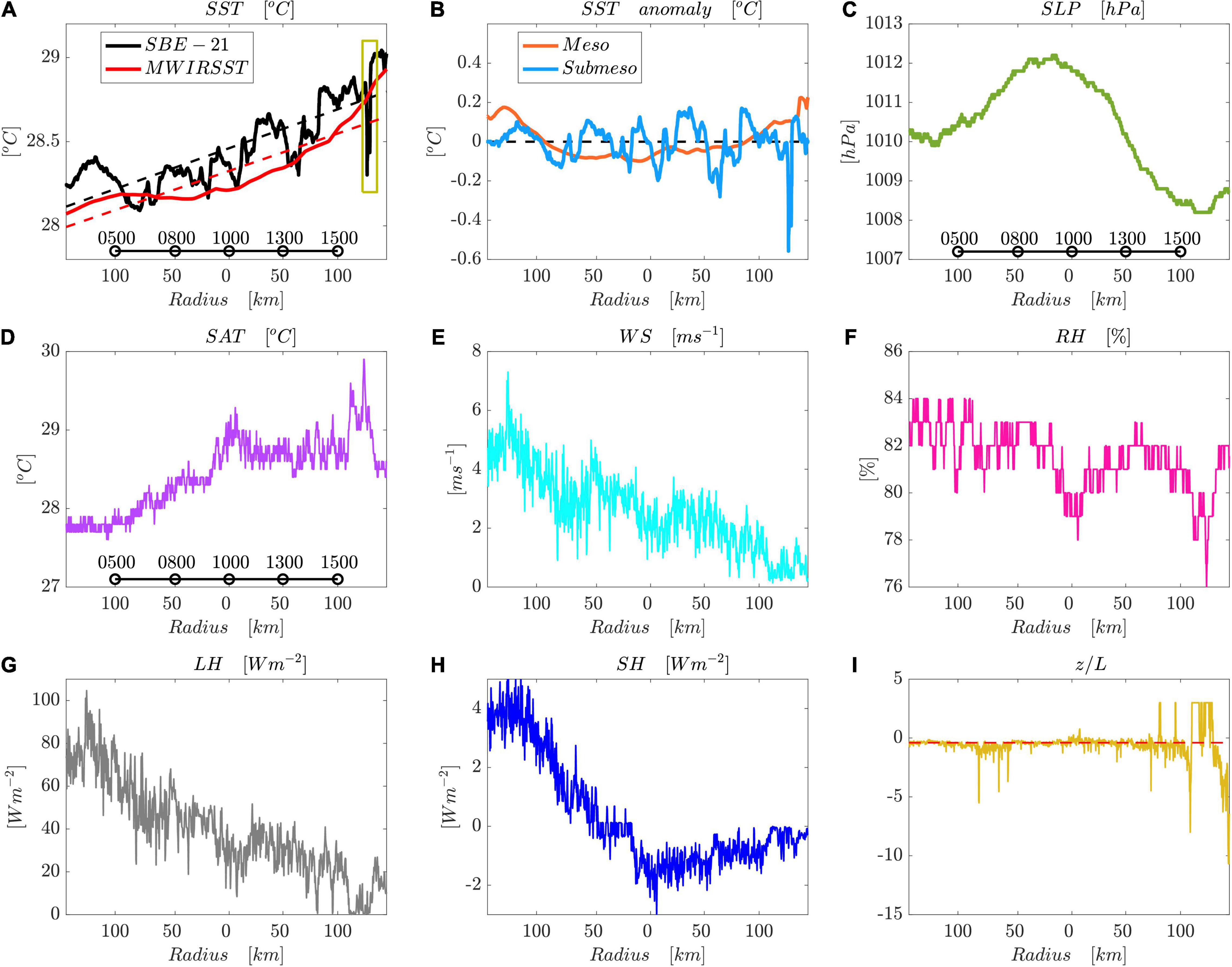
Figure 2. Cross-sectional air-sea variables across the cyclonic eddy shown in Figure 1, including the raw SST (A, unit:°C), SST anomalies (B, unit:°C), SLP (C, unit: hPa), SAT (D, unit:°C), WS (E, unit: ms^–1), RH (F, unit:%), LH (G, unit: Wm^–2), SH (H, unit: Wm^–2) and stability parameter of MABL ζ = z/L, with ζ = −0.4 denoted by dashed red lines (I). Raw SST and its linear front demonstrated by solid and dashed lines in (A), respectively. The satellite-based mean south-north SST variations (solid red) and their trend (dashed red) are averaged over 10 days before and after the cross-sectional ship observations. The yellow frame in (A) highlights the strong variations in the raw SST within a short distance. SST anomalies (B) associated with meso- and submesoscale motions are decomposed (Eq. 2) and shown by orange and blue lines, respectively. The horizontal line with black circles (A,C,D) indicates the local observation time. The x-axis represents the radius of the mesoscale eddy with the center at approximately 115.9°E, 17.3°N.

FIGURE 3

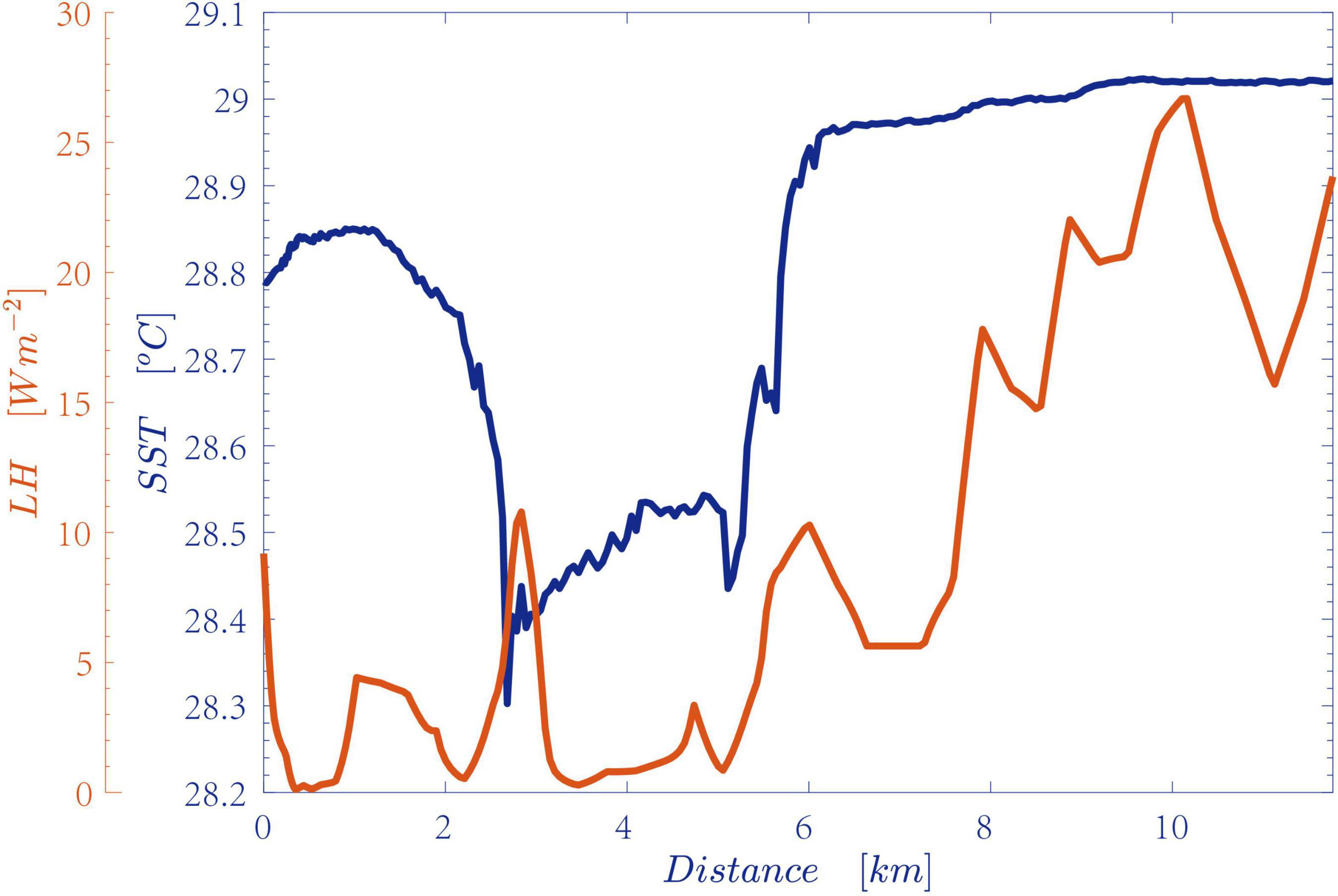
Figure 3. Enlarged plots of the anomalies in SST (blue) and LH (orange) marked by yellow frames in Figure 2A. The y-axis denotes the distances in km.

Meteorological Variables and Estimated Heat Fluxes

The sea level pressure (SLP) shows a diurnal variation (Figure 2C) that ranges from 1,008 to 1,012 hPa. A minimum pressure is found in the afternoon associated with the strongest surface heating, as indicated by the surface air temperature (SAT, Figure 2D). A maximum SAT of ∼30°C and a minimum relative humidity (RH) of 76% occur accordingly. The wind speed (WS) decreases from 7 ms^–1 to less than 1 ms^–1 when the vessel heads south. Using the above meteorological variables and the SST, the air-sea turbulent heat fluxes can be estimated by bulk formulas of the Coupled Ocean-Atmosphere Response Experiment (COARE) 3.5 (Edson et al., 2013). The heat fluxes are calculated using the absolute WS ($\left|\overline{{\mathit{\text{u}}}_{\mathit{z}}}\right|$ in Eq. 1) rather than the relative WS with reference to the surface currents because the surface currents are weak at a magnitude of ∼O(0.1) ms^–1. The estimated LH shows a significant decrease of approximately 100 Wm^–2 from north to south, following a weakened WS. Even though the LH is lower in the south with weaker WS, an anomaly in LH is approximately 25 Wm^–2 accompanied by a sudden anomaly in SST, which increases by 0.9°C within ∼3.6 km (Figure 3). The sensible heat flux ranges from −2 to 4 Wm^–2 and is associated with a weak air-sea temperature difference. The negative sensible heat flux values indicate an inverse air-sea temperature difference when the SAT is higher than the SST. Given the weak magnitude compared to the LH, sensible heat flux anomalies are not investigated in this study.

The spatial LH anomalies are predominated by the role of the WS, with a dominant weakly unstable boundary layer stability ζ = z/L, where z is the height of the turbulent exchange coefficient and L is the Obukhov length scale:

$\mathit{\text{L}}=\frac{{\mathit{\text{u}}}_{*}^2}{\mathbf{\kappa }\frac{\mathit{g}}{\overline{\mathit{T}}}{\mathit{\text{T}}}_{*}}(3)$

where κ ≈ 0.4 is the von Kármán constant, u_* denotes the frictional velocity, g is the gravitational acceleration, $\overline{\mathit{\text{T}}}$ is the mean temperature in the boundary layer, and ${\mathit{\text{T}}}_{*}=-\frac{\overline{{\mathit{w}}^{\prime }{\mathbf{\theta }}^{\prime }}}{{\mathit{u}}_{*}}$. L represents the ratio of the work done by the Reynolds stress to that done by the buoyancy forces. The MABL shows three statuses during the observational period (Figure 2I): stable (ζ > 0.1), near-neutral (−0.4 ≤ ζ ≤0.1) and unstable (ζ < −0.4). These statuses are mathematically associated with the Obukhov length scale. The unstable MABL is predominant (Figure 2I), as the SST is mostly higher than the air temperature in the vertical atmospheric profile (Figure 4). This pattern can give rise to convective processes in the boundary layer. However, the air temperature is higher than the SST during an observation at noon (1,300) at local time, exhibiting an approximate 1°C temperature difference. This causes a stabilized boundary layer condition. The mean air-sea humidity difference is approximately 5 g⋅kg^–1 regardless of the boundary layer stability. The specific humidity of the atmosphere within the cyclonic eddy is slightly lower than that in the eddy margin, with a difference of 2 g⋅kg^–1. The vertical WS at different sounding balloon release times also indicates a weak wind in the evening. Given the importance of the WS in determining the spatial LH anomalies over mesoscale eddies, questions arise as to whether SST anomalies can contribute significantly to LH anomalies.

FIGURE 4

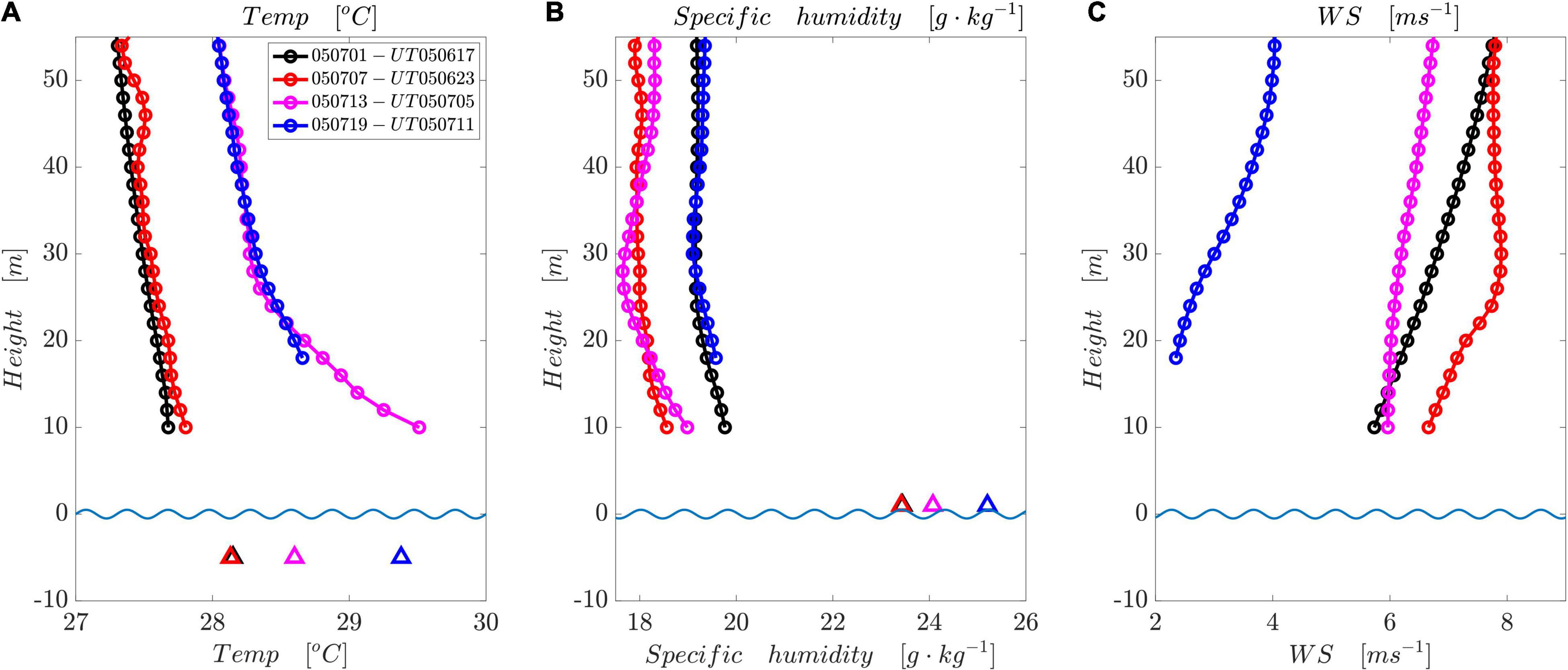
Figure 4. Vertical profiles of the following atmospheric variables: air temperature (A, unit:°C), specific humidity (B, unit: g⋅kg^–1) and WS (C, unit: ms^–1). Different colors indicate different observation locations every 6 h across the cyclonic eddy (Figure 1). Only the variables in the lower atmospheric boundary layer are shown for better visualization. The SST values are denoted by triangles with the same color as the corresponding meteorological measurements. The near-surface humidity is calculated using the SST based on saturation with a 2% reduction considering a salinity effect: q_s = 0.98×qsat(θ, SLP). The light blue wavy lines indicate the schematic sea surface.

Results

Latent Heat Flux-Sea Surface Temperature Anomalies in Association With Meso- and Submesoscale Processes

Anomalies in wind and air-sea humidity differences, along with the non-linear effect between them, give rise to LH anomalies. The WS plays a central role in determining the spatial LH anomalies for this observation with a background air-sea humidity difference. However, spatial LH anomalies across the cyclonic eddy can also be affected by the SST anomaly induced air-sea humidity difference δq = q_s − q_a = 0.98qsat(θ, SLP) − q_a (qsat means the specific humidity at saturation). To investigate the LH-SST anomalies, the following sensitivity experiments are used to estimate the anomalies caused by balanced dynamics:

${\mathit{\text{Q}}}_{{\mathit{LH}}_{\mathit{meso}}}^{\prime }={\mathit{\text{Q}}}_{\mathit{LH}}(\overline{\mathbf{\theta }}+{\mathbf{\theta }}_{\mathit{meso}})-{\mathit{\text{Q}}}_{\mathit{LH}}(\overline{\mathbf{\theta }})(4)$

The other meteorological parameters used to estimate the LH are set to be the same for ${\mathit{\text{Q}}}_{\mathit{LH}}(\overline{\mathbf{\theta }}+{\mathbf{\theta }}_{\mathit{meso}})$ and ${\mathit{\text{Q}}}_{\mathit{LH}}(\overline{\mathbf{\theta }})$. A similar relation can be used to obtain the LH anomalies associated with submesoscale processes (or large-scale linear front in Figures 1B, 2A) by replacing θ_meso with θ_submeso (θ_linear). In addition, the LH anomalies associated with the submesoscale processes can be also estimated by the following relation:

${\mathit{\text{Q}}}_{{\mathit{LH}}_{\mathit{submeso}}}^{\prime }={\mathit{\text{Q}}}_{\mathit{LH}}(\overline{\mathbf{\theta }}+{\mathbf{\theta }}_{\mathit{meso}}+{\mathbf{\theta }}_{\mathit{submeso}})-{\mathit{\text{Q}}}_{\mathit{LH}}(\overline{\mathbf{\theta }}+{\mathbf{\theta }}_{\mathit{meso}})(5)$

which includes the SST anomalies induced by mesoscale eddies. The LH is a monotonic function of the SST, which influences the near-surface water vapor (qsat). Thus, the LH anomalies estimated by the above two methods are nearly the same (not shown here to avoid repetition). Only Eq. (4) is used in the following analysis. Two kinds of sensitivity experiments are conducted using two sets of atmospheric variables. One model is forced with realistic observed parameters (Figure 5A), and the other is run with cross-sectional mean atmospheric variables (Figure 5B) to better examine the role of SST anomalies in determining the LH anomalies across the eddy.

FIGURE 5

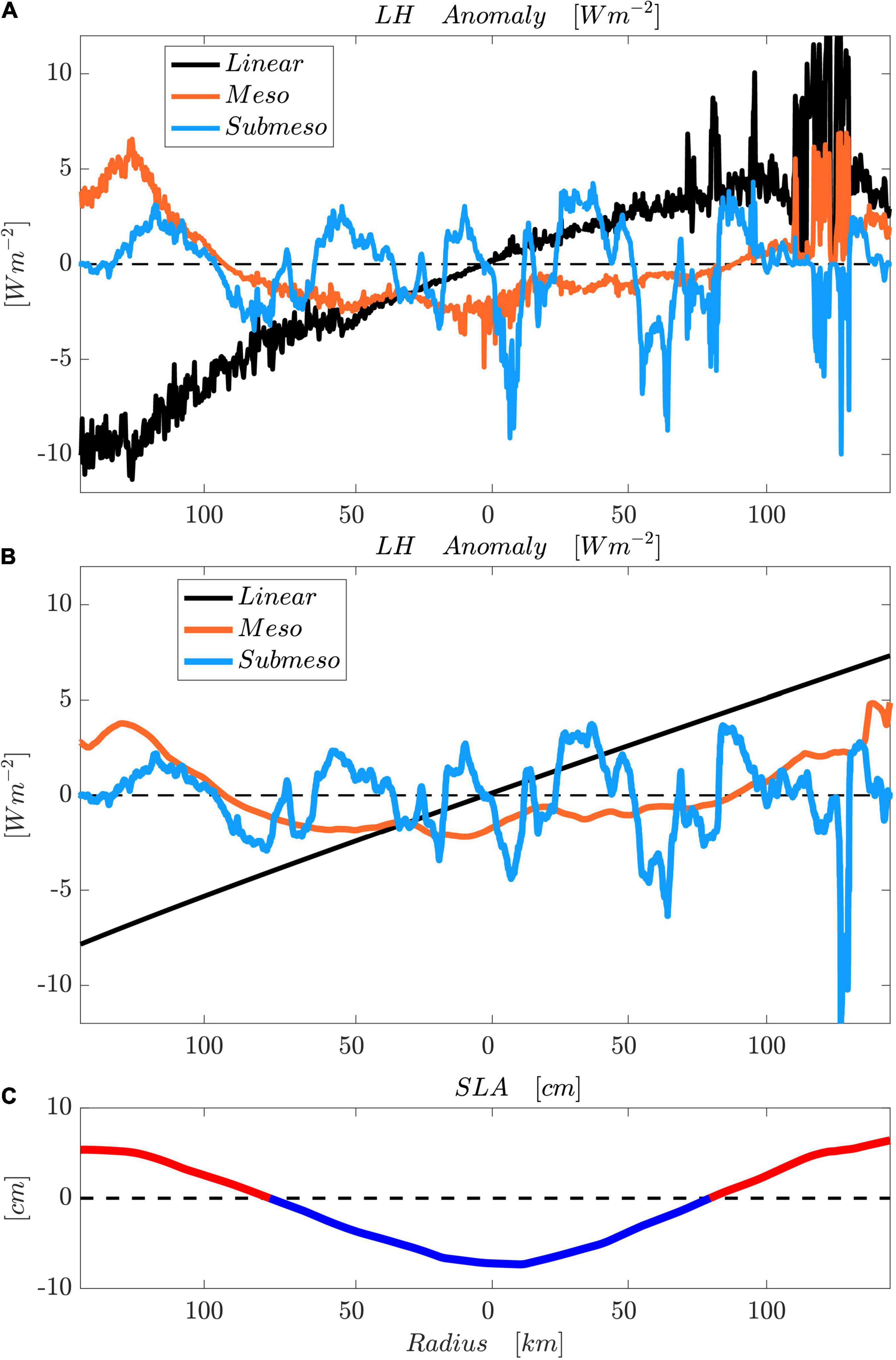
Figure 5. (A) Anomalies in the LH (unit: Wm^–2) induced by SST anomalies associated with large-scale linear fronts (black), mesoscale (orange) and submesoscale (light blue) ocean motions with realistic atmospheric parameters, including the RH, SAT, WS and SLP, as shown in Figure 2. (B) Same as in (A) but with averaged constant atmospheric variables. (C) SLA along the ship track, indicating the mesoscale eddy information using high-resolution AVISO data.

The LH anomalies resulting from the large-scale linear SST fronts are generally higher than those induced by the SST anomalies in terms of meso- and submesoscale eddies (summarized in Table 1). With realistic atmospheric variables, an amplitude of the LH (the difference between the maximum and minimum LH) anomaly of approximately 12 Wm^–2 is associated with the mesoscale eddy process, which is in accordance with the results shown in Villas Bôas et al. (2015) and Liu et al. (2020). The mesoscale eddy-induced SST anomaly accounts for 7 Wm^–2 by using the mean meteorological variables over the whole cross-section. The positive anomalies in this location (Figure 5) indicate a higher LH with a warmer sea surface. Within the eddy center, SST cooling is spatially accompanied by negative SLA and LH anomalies, which also confirms the reliability of the method provided in Eq. (4). In both cases, with realistic and mean meteorological variables, the amplitude of the LH anomaly in terms of submesoscale processes is larger than that associated with mesoscale eddies. In the case with averaged atmospheric variables, the amplitude (18.3 Wm^–2) induced by submesoscale eddies is more than twice that (7.1 Wm^–2) resulting from mesoscale processes. The observations show that the largest mean spatial gradients of the LH anomaly ($\left|{\mathit{\text{dQ}}}_{\mathit{LH}}^{\prime }/\mathit{\text{dr}}\right|$) come from the linear SST fronts (2.2 Wm^–2km^–1), followed by submeso- (1.7 Wm^–2km^–1) and mesoscale (1.2 Wm^–2km^–1) SST anomalies. The role of the submesoscale process is approximately 1.5 times that of the mesoscale eddy. However, the submesoscale process predominates over the other two processes for determining the spatial gradients of LH anomalies when the averaged atmospheric variables are used (Table 1). This confirms the significant role of the unbalanced submesoscale motions in contributing to the SST and LH anomalies. Here, we only show the cross-sectional results due to the limited observational ability. To better illustrate the LH and SST anomalies within the cyclonic eddy, we attempt to schematically show the circular structures by applying the cross-sectional values to the circular patterns (Figure 6). This is based on the assumption that the cross-sectional observations are representative of the meso- and submesoscale structures, which provides a rough observational reference for the existing reanalysis results (e.g., Villas Bôas et al., 2015) and future works.

TABLE 1

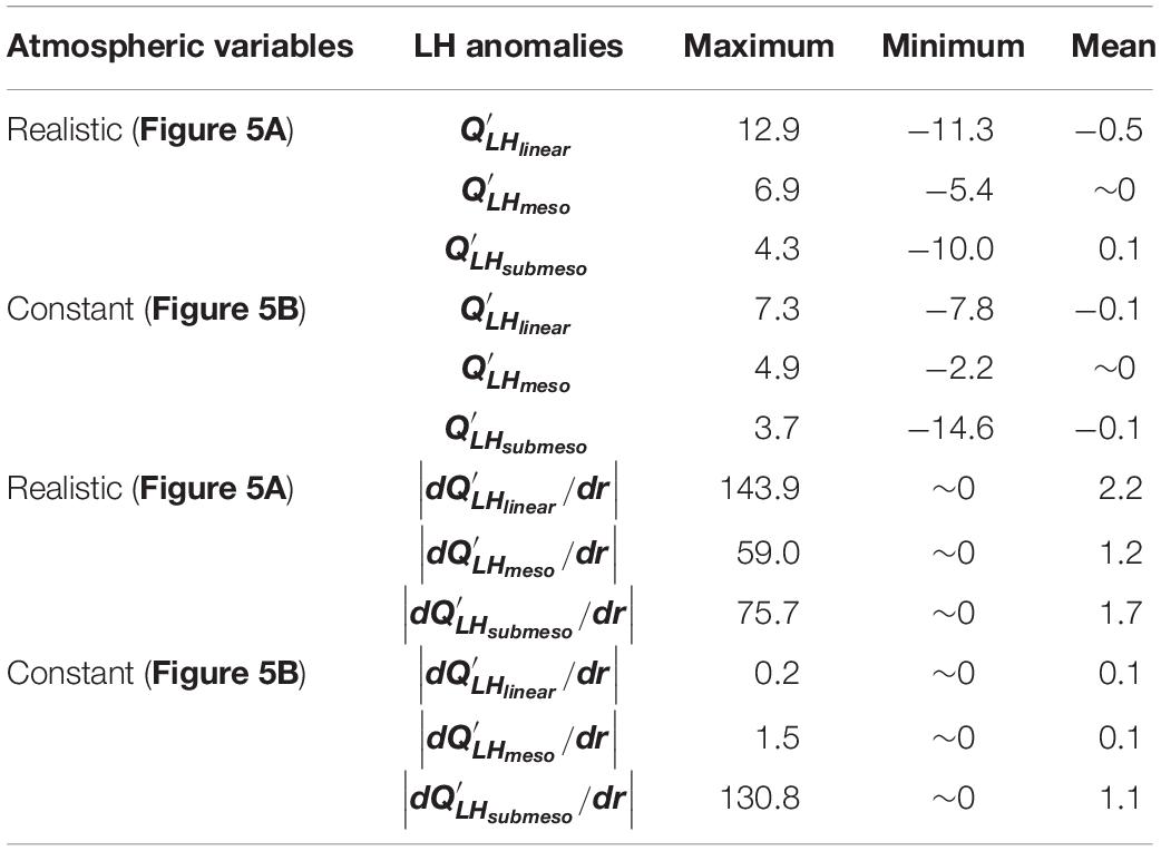
Table 1. Summary of the decomposed LH anomalies (${\mathit{\text{Q}}}_{\mathit{LH}}^{\prime }$, unit: Wm^–2) and their spatial gradients ($\left|{\mathit{\text{dQ}}}_{\mathit{LH}}^{\prime }/\mathit{\text{dr}}\right|$, unit: Wm^–2km^–1) resulting from SST anomalies associated with large-scale linear fronts and meso- and submesoscale motions.

FIGURE 6

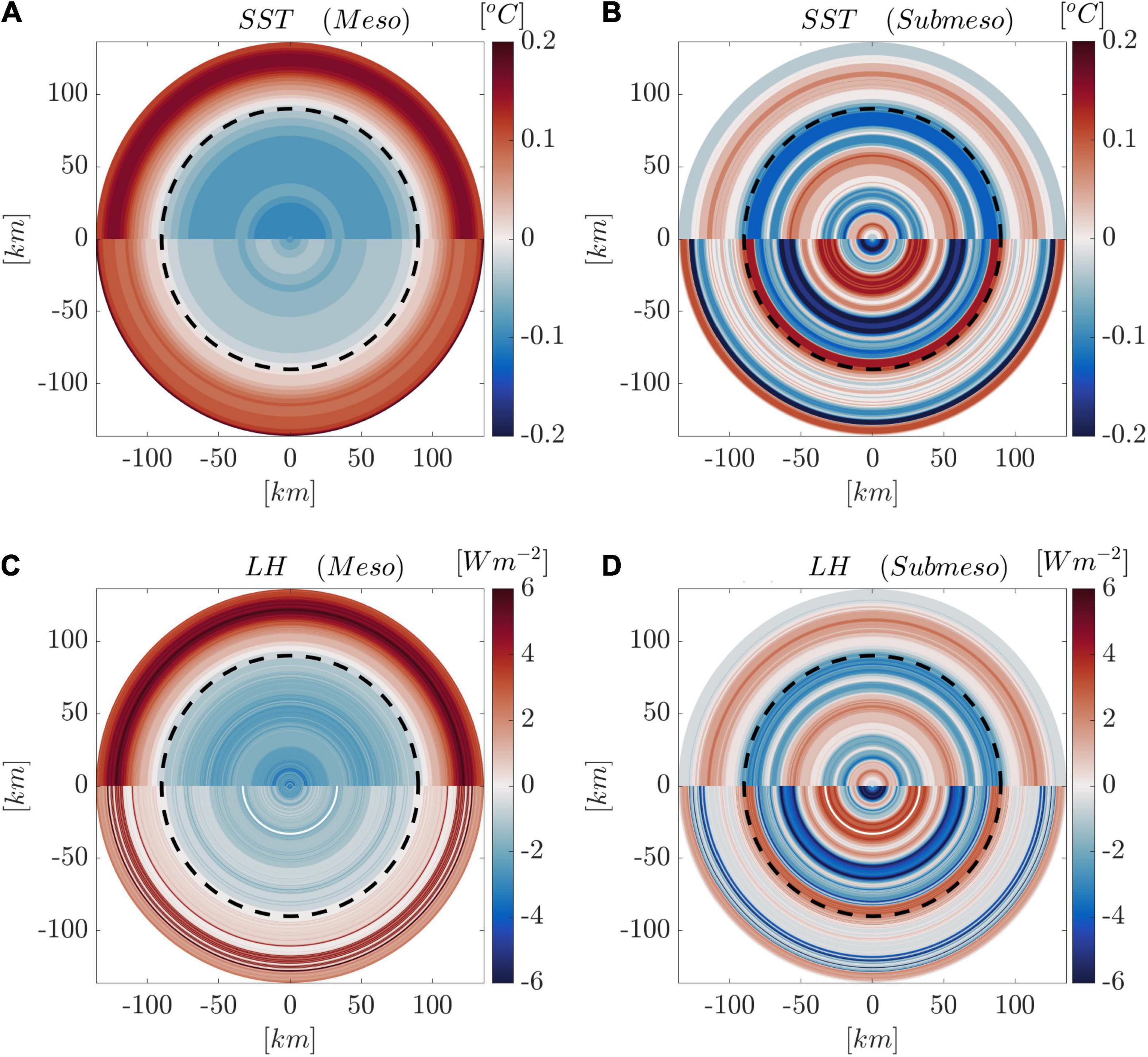
Figure 6. Schematic circular patterns of anomalies in SST (A,B) and LH (C,D) induced by meso- and submesoscale processes applying cross-sectional observations to circular structures. The black dashed circular rings indicate the radius of the cyclonic eddy at approximately 90 km.

Spectral Analysis of Latent Heat Flux and Sea Surface Temperature Anomalies

Spectral analysis is used to investigate the underlying mechanism and identify the scale at which these variations are most active. The spectrum of the SST anomalies shows a peak at ∼15 km (Figure 7A), indicative of noticeable submesoscale fronts/filaments at the surface. Spiral-like filaments exist in mesoscale eddies, which is a typical submesoscale feature, as revealed by high-resolution satellite observations (e.g., McWilliams, 2016) and numerical simulations (Brannigan et al., 2017) of mesoscale eddies. Our survey traversing the eddy coincidentally captured these surface features. Interestingly, the spectrum of the LH anomalies shows a similar shape with peak variance at ∼15 km (Figure 7B), as evidence for the underlying relationship between the lateral LH variability and submesoscale process. At smaller scales, both the SST and LH spectra present a slowly flattening slope from the k^–3 to k^–2 power law, indicating more active variability at smaller scales. As there seems to be no additional mechanism for the submesoscale variability of LH, the submesoscale SSH variance—a proxy for submesoscale dynamics—should be the causation of the dramatic LH variability at submesoscales. The effect of air-sea interactions at submesoscales may also be linked to submesoscale dynamics in the ocean interior where submesoscale turbulence is energetic [we reveal upper ocean submesoscale instabilities driven by internal wave shear in a twin study (Song et al., 2022)]. In addition, underwater submesoscale dynamics can be an important dynamic mechanism for vertical heat transport into the deep ocean (Su et al., 2018, 2020; Cao and Jing, 2022).

FIGURE 7

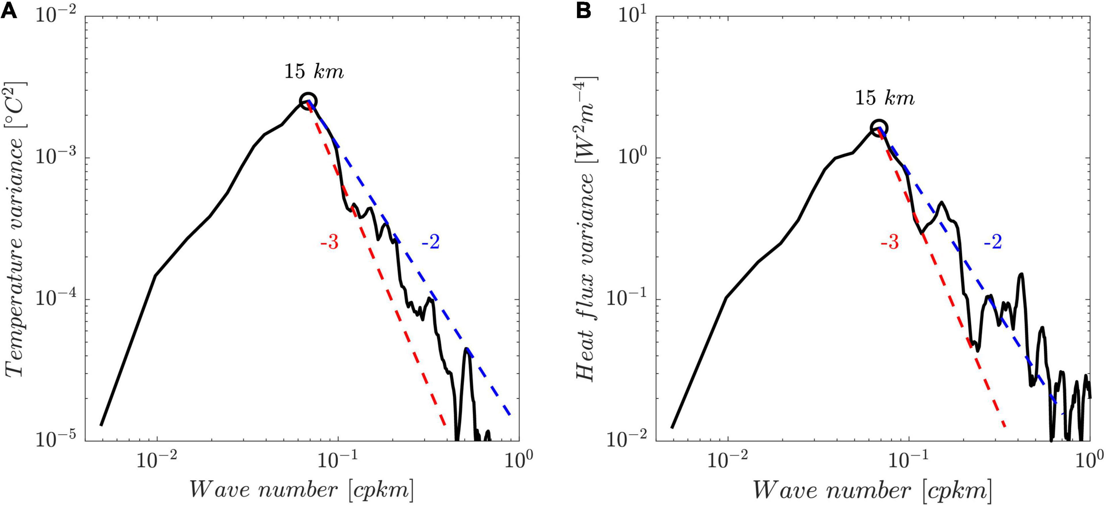
Figure 7. Power spectral densities (PSDs) of the (A) SST anomalies (Figure 2B, blue) and (B) LH anomalies (Figure 5A, blue) associated with unbalanced submesoscale motions. The peak wavelengths are marked by circles. The slopes of k^–2 (dashed blue) and k^–3 (dashed red) are incorporated for reference.

Discussion

LH anomalies with magnitudes of ∼O(10) Wm^–2 can be caused by SST anomalies in association with mesoscale eddies. However, less attention is devoted to the surface LH anomalies induced by unbalanced submesoscale motions due to the high requirement of spatial and temporal observations. Using the measurements across the center of a cyclonic eddy from a satellite-ship-coordinated cruise, this paper presents the observational results of a comparison of LH anomalies induced by balanced mesoscale and unbalanced submesoscale eddies. Two major findings can be briefly summarized. (i) Strong SST fronts and instabilities resulting from meso- and submesoscale motions are observed; these fronts and instabilities can determine the LH anomalies by changing the near-surface humidity and air-sea humidity difference. The amplitude of LH anomalies induced by submesoscale processes is 2 Wm^–2 higher than those generated by mesoscale eddies. However, the spatial gradients of the former are 1.5 times those of the latter. The mean (maximum) spatial gradient values are 1.7 (75.7) Wm^–2km^–1 and 1.2 (59.9) Wm^–2km^–1 for unbalanced and balanced motions, respectively. (ii) The similar spectral shapes and peaks (∼15 km) of the SST and LH anomalies suggest that submesoscale dynamics are likely the causation of the dramatic LH variability at the submesoscale. The air-sea interaction may also be affected by submesoscale processes in the ocean interior (Song et al., 2022).

Scientists have already started revolving mesoscale investigations of air-sea heat fluxes based on eddy-resolving reanalysis and have objectively analyzed products at a spatial resolution of one quarter of a degree. However, the current heat flux estimates from various platforms still contain considerable uncertainties, with an approximate global imbalance at 10–20 Wm^–2, as reviewed by Yu (2019). This imbalance may be attributed to errors in air-sea variables and different calculation algorithms. The above two reasons may be future solutions for the global surface heat flux budget balance. This paper provides an observational case study showing significant spatial differences across a cyclonic eddy. These differences can result in spatial uncertainties in air-sea variables and heat fluxes if the spatial resolution is not properly resolved. The spectral analysis in this study shows a spatial peak at ∼15 km, which indicates that one quarter of a degree may not be sufficient to produce future heat flux estimates. This finding suggests that an appropriate increase in the spatial resolution provides an optional way to balance the heat budget, which of course requires great effort from the heat flux community.

It should be noted that this case study provides only snapshot-like estimates of LH anomalies in association with meso- and submesoscale motions and still gives a limited view of the full process of the LH anomalies due to the limitation of the observational ability. The dynamic link between the meso- and submesoscale processes giving rise to anomalies in SST and LH remains unrevealed. We also have to admit that the decomposition of the SST anomalies into different scales (Eq. 2) is imperfect due to the possible mesoscale non-linear effects. Therefore, the results in this paper only quantitatively highlight the considerable LH anomalies induced by submesoscale processes. Two major points of evidence provide supports to validate the results, which to a certain extent enhances our confidence in using the SST decomposition method. First, the decomposed mesoscale signal of SST in space is in accordance with the geometrical features of the cyclonic eddy in terms of SLA, as shown in Figures 5, 6. Second, the spectra of the anomalies of both SST and LH exhibit a peak at ∼15 km (Figure 7), indicating a notable submesoscale process at the surface. In this study, we attempt to caution the contribution of the high spatial resolution in understanding the heat flux variations beyond the mesoscale eddy-resolving ability.

The LH anomalies, in association with the pronounced variations between positive and negative temperature anomalies, can lead to uncertainties/difficulties in estimating the mean LH averaged over standard latitudinal grids along the observational cross-section. For example, the 0.25° grids in models (e.g., ERA5) are appropriate for resolving mesoscale effects; however, the spatial effects of submesoscale processes may not be evident at this scale. Figure 8 shows the spatial mean LH anomalies (${\mathit{\text{Q}}}_{\mathit{LH}}^{\prime }$) induced by meso- and submesoscale processes and the mean LH in association with large-scale south-north SST fronts ($\overline{{\mathit{\text{Q}}}_{{\mathit{LH}}_{\mathit{linear}}}}$) without meso- and submesoscale effects in each 0.25 grid from 18.25°N to 16.25°N. The gross impacts of the meso- and submesoscale processes in producing heat fluxes can be quantitatively understood at the grid scale. On average, the mean LH anomaly in all grids associated with the (sub) mesoscale eddy is (2.4) 1.4 Wm^–2 in this observational case, with an averaged percentage (6) 4% compared to the mean LH ($\overline{{\mathit{\text{Q}}}_{{\mathit{LH}}_{\mathit{linear}}}}$). In addition, the mean maximum LH anomaly in all grids associated with the (sub) mesoscale eddy is (10) 7 Wm^–2, with a mean ratio (19) 12%. On average, the role of the submesoscale process is comparable to and slightly more dominant than that of the mesoscale eddy process. The ratios above increase from north to south as a result of the decreased mean LH due to the weakened wind speed (Figure 2). However, it should be noted here that the results shown here are still case dependent. More efforts and observations are required to systematically investigate this question.

FIGURE 8

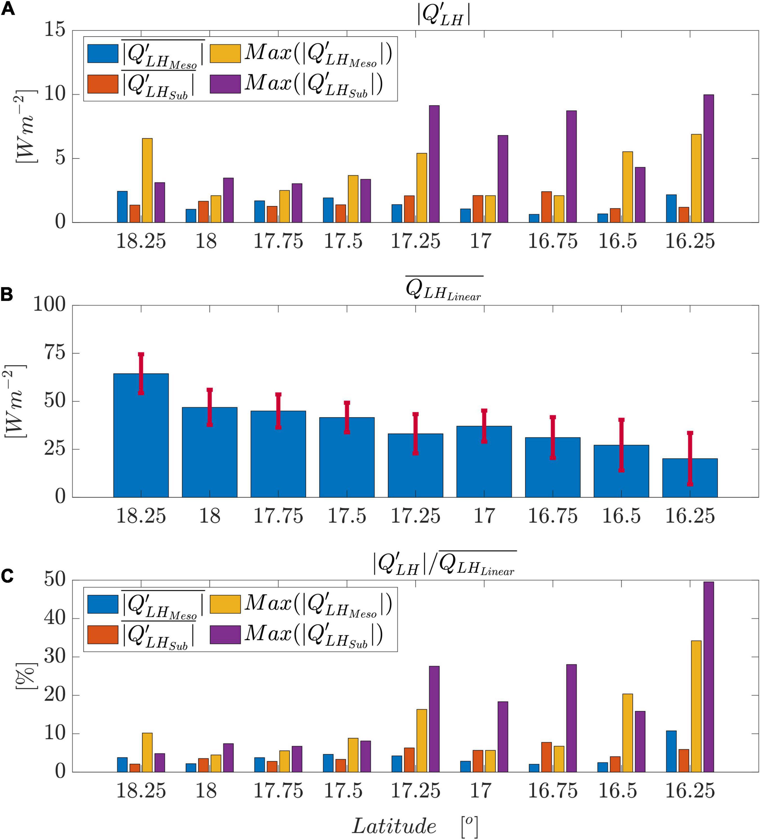
Figure 8. The mean LH anomalies ($\left|{\mathit{\text{Q}}}_{\mathit{LH}}^{\prime }\right|$) induced by meso- (blue and yellow bars) and submesoscale (red and purple bars) processes averaged over standard latitudinal grids with a spatial interval of 0.25°. (A) The mean absolute values of the anomalies along with the maximum values (yellow and purple bars) induced by meso- and submesoscale processes (summarized numbers of Figure 5A). (B) The mean LH ($\overline{{\mathit{\text{Q}}}_{{\mathit{LH}}_{\mathit{linear}}}}$) in each latitudinal grid estimated based on realistic atmospheric variables and linear south-north SST fronts (θ_linear) without meso- and submesoscale effects. The errorbars (red) indicate the standard deviations for spatially averaged grid values. (C) The ratio (percentage) of the mean LH anomaly ($\left|{\mathit{\text{Q}}}_{\mathit{LH}}^{\prime }\right|$, A) to the mean LH ($\overline{{\mathit{\text{Q}}}_{{\mathit{LH}}_{\mathit{linear}}}}$, B) in each grid.

This study shows only a single-way process without investigating the air-sea feedbacks and the damping of the SST in terms of the LH. This paper shows the results in early summer; thus, the results of LH anomalies in association with unbalanced submesoscale processes may be underestimated. First, the role of SST anomalies in contributing to LH anomalies may be weakened with weak and near-neutral boundary layer stability. In winter, the air-sea humidity difference as a function of the SST should be dominant in determining LH anomalies with a strongly unstable MABL. Second, the submesoscale instabilities in the mixed layer show significant seasonality (Mensa et al., 2013; Qiu et al., 2014; Sasaki et al., 2014; Callies et al., 2015; Thompson et al., 2016), with stronger intensity in winter but weaker intensity in summer. Thus, it is supposed that the role of unbalanced submesoscale processes with respect to balanced mesoscale eddies should be larger in winter than in summer. Further experiments will be conducted in the near future to show the seasonality.

Data Availability Statement

Publicly available datasets were analyzed in this study. This data can be found here: The observational data can be found at http://www.ocean.iap.ac.cn/. High-resolution SLA data are provided by the State Oceanic Administration (SOA).

Author Contributions

XS led the analyses, the conception, and writing of the manuscript. XS and WY constructed the SCS cruise. BQ, S-PX, XX, HC, and ZC gave input to the analysis process. All authors have read, commented, and agreed to the manuscript before submission.

Funding

This study was funded by the National Natural and Science Foundation of China (42122040, 42076016, and 42176004). The authors acknowledge the cruise supported by the Southern Marine Science and Engineering Guangdong Laboratory (Zhuhai) (311021001).

Conflict of Interest

The authors declare that the research was conducted in the absence of any commercial or financial relationships that could be construed as a potential conflict of interest.

Publisher’s Note

All claims expressed in this article are solely those of the authors and do not necessarily represent those of their affiliated organizations, or those of the publisher, the editors and the reviewers. Any product that may be evaluated in this article, or claim that may be made by its manufacturer, is not guaranteed or endorsed by the publisher.

Acknowledgments

We appreciate the constructive comments from the reviewers.

Footnotes

1. ^ www.seabird.com/
2. ^ www.vaisala.com/en

References

Barkan, R., Winters, K. B., and McWilliams, J. C. (2017). Stimulated imbalance and the enhancement of eddy kinetic energy dissipation by internal waves. J. Phys. Oceanogr. 47, 181–198. doi: 10.1175/JPO-D-16-0117.1

CrossRef Full Text | Google Scholar

Brannigan, L., Marshall, D. P., Naveira Garabato, A. C., Nurser, A. J. G., and Kaiser, J. (2017). Submesoscale Instabilities in Mesoscale Eddies. J. Phys. Oceanogr. 47, 3061–3085. doi: 10.1175/JPO-D-16-0178.1

CrossRef Full Text | Google Scholar

Callies, J., Ferrari, R., Klymak, J. M., and Gula, J. (2015). Seasonality in submesoscale turbulence. Nat. Commun. 6:6862. doi: 10.1038/ncomms7862

PubMed Abstract | CrossRef Full Text | Google Scholar

Cao, H., and Jing, Z. (2022). Submesoscale ageostrophic motions within and below the mixed layer of the northwestern Pacific Ocean. J. Geophys. Res. 127, e2021JC017812. doi: 10.1029/2021JC017812

CrossRef Full Text | Google Scholar

Carton, J. A., and Zhou, Z. (1997). Annual cycle of sea surface temperature in the tropical Atlantic Ocean. J. Geophys. Res. 102, 27813–27824. doi: 10.1029/97JC02197

CrossRef Full Text | Google Scholar

Cayan, D. R. (1992). Latent and Sensible Heat Flux Anomalies over the Northern Oceans: Driving the Sea Surface Temperature. J. Phys. Oceanogr. 22, 859–881. doi: 10.1175/1520-04851992022<0859:LASHFA<2.0.CO;2

CrossRef Full Text | Google Scholar

Chelton, D. B., DeSzoeke, R. A., Schlax, M. G., El Naggar, K., and Siwertz, N. (1998). Geographical variability of the first baroclinic Rossby radius of deformation. J. Phys. Oceanogr. 28, 433–460. doi: 10.1175/1520-04851998028<0433:GVOTFB<2.0.CO;2

CrossRef Full Text | Google Scholar

Chelton, D. B., Schlax, M. G., and Samelson, R. M. (2011). Global observations of nonlinear mesoscale eddies. Prog. Oceanogr. 91, 167–216. doi: 10.1016/j.pocean.2011.01.002

CrossRef Full Text | Google Scholar

Chelton, D. B., and Xie, S. (2010). Coupled ocean-atmosphere interaction at oceanic mesoscales. Oceanography 23, 52–69. doi: 10.5670/oceanog.2010.05

CrossRef Full Text | Google Scholar

Clayson, C. A., and Edson, J. B. (2019). Diurnal surface flux variability over western boundary currents. Geophys. Res. Lett. 46, 9174–9182. doi: 10.1029/2019GL082826

CrossRef Full Text | Google Scholar

Edson, J. B., Jampana, V., Weller, R. A., Bigorre, S. P., Plueddemann, A. J., Fairall, C. W., et al. (2013). On the exchange of momentum over the open ocean. J. Phys. Oceanogr. 43, 1589–1610. doi: 10.1175/JPO-D-12-0173.1

CrossRef Full Text | Google Scholar

Fairall, C. W., Bradley, E. F., Hare, J. E., Grachev, A. A., and Edson, J. B. (2003). Bulk parameterization of air-sea fluxes: Updates and verification for the COARE algorithm. J. Climate 16, 571–591. doi: 10.1175/1520-04422003016<0571:BPOASF<2.0.CO;2

CrossRef Full Text | Google Scholar

Falkowski, P. G., Ziemann, D., Kolber, Z., and Bienfang, P. K. (1991). Role of eddy pumping in enhancing primary production in the ocean. Nature 352, 55–58. doi: 10.1038/352055a0

CrossRef Full Text | Google Scholar

Ferrari, R., and Wunsch, C. (2009). Ocean Circulation Kinetic Energy: Reservoirs, Sources, and Sinks. Annu. Rev. Fluid Mech. 41, 253–282. doi: 10.1146/annurev.fluid.40.111406.102139

CrossRef Full Text | Google Scholar

Foltz, G. R., and McPhaden, M. J. (2005). Mixed layer heat balance on intraseasonal time scales in the northwestern tropical Atlantic Ocean. J. Climate 18, 4168–4184. doi: 10.1175/JCLI3531.1

CrossRef Full Text | Google Scholar

Frenger, I., Gruber, N., Knutti, R., and Münnich, M. (2013). Imprint of Southern Ocean eddies on winds, clouds and rainfall. Nat. Geosci. 6, 608–612. doi: 10.1038/ngeo1863

CrossRef Full Text | Google Scholar

Gaube, P., Chelton, D. B., Samelson, R. M., Schlax, M. G., and O’Neill, L. W. (2015). Satellite observations of mesoscale eddy-induced Ekman pumping. J. Phys. Oceanogr. 45, 104–132. doi: 10.1175/JPO-D-14-0032.1

CrossRef Full Text | Google Scholar

Hall, A., and Visbeck, M. (2002). Synchronous variability in the Southern Hemisphere atmosphere, sea ice, and ocean resulting from the annular mode. J. Climate 15, 3043–3057. doi: 10.1175/1520-04422002015<3043:SVITSH<2.0.CO;2

CrossRef Full Text | Google Scholar

Hausmann, U., and Czaja, A. (2012). The observed signature of mesoscale eddies in sea surface temperature and the associated heat transport. Deep Sea Res. 70, 60–72. doi: 10.1016/j.dsr.2012.08.005

CrossRef Full Text | Google Scholar

Hurrell, J. W., and Deser, W. C. (2009). North Atlantic climate variability: The role of the North Atlantic Oscillation. J. Mar. Syst. 79, 231–244. doi: 10.1016/j.jmarsys.2009.11.002

CrossRef Full Text | Google Scholar

Ito, T., Woloszyn, M., and Mazloff, M. (2010). Anthropogenic carbon dioxide transport in the Southern Ocean driven by Ekman flow. Nature 463, 80–83. doi: 10.1038/nature08687

PubMed Abstract | CrossRef Full Text | Google Scholar

Large, W. G., and Pond, S. (1981). Open ocean momentum flux measurements in moderate to strong winds. J. Phys. Oceanogr. 11, 324–336. doi: 10.1175/1520-04851981011<0324:OOMFMI<2.0.CO;2

CrossRef Full Text | Google Scholar

Lin, I., Chen, C., Pun, I., Liu, W., and Wu, C. (2009). Warm ocean anomaly, air sea Fluxes, and the rapid intensification of tropical cyclone Nargis (2008). Geophys. Res. Lett. 36, L03817. doi: 10.1029/2008GL035815

CrossRef Full Text | Google Scholar

Liu, W. T., Katsaros, K. B., and Businger, J. A. (1979). Bulk parameterization of air-sea exchanges of heat and water vapor including the molecular constraints at the interface. J. Atmos. Sci. 36, 1722–1735. doi: 10.1175/1520-04691979036<1722:BPOASE<2.0.CO;2

CrossRef Full Text | Google Scholar

Liu, Y., Yu, L., and Chen, G. (2020). Characterization of sea surface temperature and air-sea heat flux anomalies associated with mesoscale eddies in the South China Sea. J. Geophys. Res. 125, e2019JC015470. doi: 10.1029/2019JC015470

CrossRef Full Text | Google Scholar

Marshall, J., Kushnir, Y., Battisti, D., Chang, P., Czaja, A., Dickson, R., et al. (2001). North Atlantic climate variability, phenomena, impacts and mechanisms. Int. J. Climatol. 21, 1863–1898. doi: 10.1002/joc.693

CrossRef Full Text | Google Scholar

McWilliams, J. C. (2016). Submesoscale currents in the ocean. Proc. R. Soc. A 472, 20160117. doi: 10.1098/rspa.2016.0117

PubMed Abstract | CrossRef Full Text | Google Scholar

Mensa, J. A., Garraffo, Z., Griffa, A., Ozgokmen, T. M., Haza, A., and Veneziani, M. (2013). Seasonality of the submesoscale dynamics in the Gulf Stream region. Ocean Dyn. 63, 923–941. doi: 10.1007/s10236-013-0633-1

CrossRef Full Text | Google Scholar

Monin, A. S., and Obukhov, A. M. (1954). Basic regularity in turbulent mixing in the surface layer of the atmosphere. Tr. Geofiz. Inst. Akad. Nauk SSSR 24, 163–187.

Google Scholar

Murray, F. W. (1986). On the computation of saturation vapor pressure. J. Climate Appl. Meteor. 6, 203–204.

Google Scholar

Oke, P. R., and England, M. H. (2004). Oceanic response to changes in the latitude of the Southern Hemisphere subpolar westerly winds. J. Climate 17, 1040–1054. doi: 10.1175/1520-04422004017<1040:ORTCIT<2.0.CO;2

CrossRef Full Text | Google Scholar

Qiu, B., Chen, S., Klein, P., Sasaki, H., and Sasai, Y. (2014). Seasonal mesoscale and submesoscale eddy variability along the North Pacific Subtropical Countercurrent. J. Phys. Oceanogr. 44, 3079–3098. doi: 10.1175/JPO-D-14-0071.1

CrossRef Full Text | Google Scholar

Qu, T. (2001). Role of ocean dynamics in determining the mean season cycle of the South China Sea surface temperature. J. Geophys. Res. 106, 6943–6955. doi: 10.1029/2000JC000479

CrossRef Full Text | Google Scholar

Sasaki, H., Klein, P., Qiu, B., and Sasai, Y. (2014). Impact of oceanicscale interactions on the seasonal modulation of ocean dynamics by the atmosphere. Nat. Commun. 5:5636. doi: 10.1038/ncomms6636

PubMed Abstract | CrossRef Full Text | Google Scholar

Siegelman, L., Klein, P., Rivière, P., Thompson, A. F., Torres, H. S., Flexas, M., et al. (2020). Enhanced upward heat transport at deep submesoscale ocean fronts. Nat. Geosci. 13, 50–55. doi: 10.1038/S41561-019-0489-1

CrossRef Full Text | Google Scholar

Smith, S. D. (1988). Coefficients for sea surface wind stress, heat flux and wind profiles as a function of wind speed and temperature. J. Geophys. Res. 93, 15467–15472. doi: 10.1029/JC093iC12p15467

CrossRef Full Text | Google Scholar

Song, X. (2020). The importance of relative wind speed in estimating air-sea turbulent heat fluxes in bulk formulas: Examples in the Bohai Sea. J. Atmos. Oceanic Technol. 37, 589–603. doi: 10.1175/JTECH-D-20-0094.1

CrossRef Full Text | Google Scholar

Song, X., Cao, H., Qiu, B., Wang, W., and Yu, W. (2022). Observed subsurface imbalance stimulated in a mesoscale eddy in the South China Sea. J. Geophys. Res.

Google Scholar

Song, X., Ning, C., Duan, Y., Wang, H., Li, C., Yang, Y., et al. (2021). Observed extreme air-sea heat flux variations during three tropical cyclones in the tropical southeastern Indian Ocean. J. Climate 34, 3683–3705. doi: 10.1175/JCLI-D-20-0170.1

CrossRef Full Text | Google Scholar

Song, X., and Yu, L. (2012). High-latitude contributions to global air-sea sensible heat flux. J. Climate 25, 3515–3531. doi: 10.1175/JCLI-D-11-00028.1

CrossRef Full Text | Google Scholar

Su, Z., Torres, H., Klein, P., Thompson, A. F., Siegelman, L., Wang, J., et al. (2020). High-frequency submesoscale motions enhance the upward vertical heat transport in the global ocean. J. Geophys. Res. 125:e2020JC016544. doi: 10.1029/2020JC016544

CrossRef Full Text | Google Scholar

Su, Z., Wang, J., Klein, P., Thompson, A. F., Siegelman, L., Wang, J., et al. (2018). Ocean submesoscales as a key component of the global heat budget. Nat. Commun. 9:775. doi: 10.1038/s41467-018-02983-w

PubMed Abstract | CrossRef Full Text | Google Scholar

Thomas, L. N., Taylor, J. R., D’Asaro, E. A., Lee, C. M., Klymak, J. M., and Shcherbina, A. (2016). Symmetric instability, inertial oscillations, and turbulence at the Gulf Stream front. J. Phys. Oceanogr. 46, 197–217. doi: 10.1175/JPO-D-15-0008.1

CrossRef Full Text | Google Scholar

Thompson, A. F., Lazar, A., Buckingham, C., Garabato, A. C. N., Damerell, G. M., and Heywood, K. J. (2016). Open-ocean submesoscale motions: a full seasonal cycle of mixed layer instabilities from Gliders. J. Phys. Oceanogr. 46, 1285–1307. doi: 10.1175/JPO-D-15-0170.1

CrossRef Full Text | Google Scholar

Trenberth, K. E., Fasullo, J. T., and Kiehl, J. (2009). Earth’s global energy budget. Bull. Amer. Meteor. Soc. 90, 311–323. doi: 10.1175/2008BAMS2634.1

CrossRef Full Text | Google Scholar

Villas Bôas, A. B., Sato, O. T., Chaigneau, A., and Castelão, G. P. (2015). The signature of mesoscale eddies on the air-sea turbulent heat fluxes in the South Atlantic Ocean. Geophys. Res. Lett. 42, 1856–1862. doi: 10.1002/2015GL063105

CrossRef Full Text | Google Scholar

Visbeck, M., Chassignet, E. P., Curry, R. G., Delworth, T. L., Dickson, R. R., and Krahmann, G. (2003). “The ocean’s response to North Atlantic Oscillation variability,” in The North Atlantic Oscillation: Climatic Significance and Environmental Impact, eds J. W. Hurrell, Y. Kushnir, G. Ottersen, and M. Visbeck (Washington, DC: American Geophysical Union), 134, 113–145. doi: 10.1029/134GM06GM06

CrossRef Full Text | Google Scholar

Wang, C., Wang, W., Wang, D., and Wang, Q. (2006). Interannual variability of the South China Sea associated with El Niño. J. Geophys. Res. 111:C03023. doi: 10.1029/2005JC003333

CrossRef Full Text | Google Scholar

Yan, Y., Zhang, L., Song, X., Wang, G., and Chen, C. (2021). Diurnal variation in surface latent heat flux and the effect of diurnal variability on the climatological latent heat flux over the tropical oceans. J. Phys. Oceanogr. 51, 3401–3415. doi: 10.1175/JPO-D-21-0128.1

CrossRef Full Text | Google Scholar

Yu, L. (2007). Global variations in oceanic evaporation (1958-2005): The role of the changing wind speed. J. Climate 20, 5376–5390. doi: 10.1175/2007JCLI1714.1

CrossRef Full Text | Google Scholar

Yu, L. (2019). Global air-sea fluxes of heat, fresh water, and momentum: Energy budget closure and unanswered questions. Annu. Rev. Mar. Sci. 11, 227–248. doi: 10.1146/annurev-marine-010816-060704

PubMed Abstract | CrossRef Full Text | Google Scholar

Yu, X., Naveira Garabato, A. C., Martin, A. P., Evans, D. G., and Su, Z. (2019). Wind-forced symmetric instability at a transient mid-ocean front. Geophys. Res. Lett. 46, 11281–11291. doi: 10.1029/2019GL084309

CrossRef Full Text | Google Scholar