 Aksel Alstad Mogstad
 Håvard Snefjellå Løvås
 Øystein Sture2
 Geir Johnsen
 Martin Ludvigsen
- 1Centre for Autonomous Marine Operations and Systems, Department of Biology, Norwegian University of Science and Technology (NTNU), Trondheim, Norway
- 2Centre for Autonomous Marine Operations and Systems, Department of Marine Technology, Norwegian University of Science and Technology (NTNU), Trondheim, Norway
- 3Arctic Biology Department, University Centre in Svalbard (UNIS), Longyearbyen, Norway
On the Tautra Ridge – a 39-100 m deep morainic sill located in the middle of the Trondheimsfjord, Norway – some of the world’s shallowest known occurrences of the scleractinian cold-water coral (CWC) Desmophyllum pertusum can be found. The earliest D. pertusum records from the Tautra Ridge date back to the 18th century, and since then, the location has provided easy access to physical coral specimens for numerous scientific studies. In 2013, the ridge was declared a marine protected area by the Norwegian Government due to its unique CWC reefs. However, few attempts have to our knowledge yet been made to characterize the distribution, extent and condition of these reefs extensively. The aim of the current study was therefore to add geospatial context to the Tautra CWC reef complex. In the study, data from multibeam echo sounding, synthetic aperture sonar imaging and underwater hyperspectral imaging are used to assess CWC reef occurrences from multiple perspectives. The study demonstrates how complementary remote sensing techniques can be used to increase knowledge generation during seafloor mapping efforts. Ultimately, predictive modeling based on seafloor geomorphometry is used to estimate both distribution and areal coverage of D. pertusum reefs along the majority of the Tautra Ridge. Our findings suggest that D. pertusum reef distribution on the Tautra Ridge is affected by several geomorphometric seafloor properties, and that the total reef extent in the area likely is close to 0.64 km2. Better description of current patterns across the Tautra Ridge will improve our understanding of the interaction between hydrography and geomorphology at the Tautra CWC reef complex in the future.
1 Introduction
Situated between 63°40’N 9°45’E and 64°0’N 11°30’E, the 135 km long Trondheimsfjord is one of Norway’s largest fjord systems. The fjord system consists of three main basins: the 617 m deep outer basin, the 440 m deep middle basin and the 270 m deep inner basin (Jacobson, 1983). These basins – respectively denoted as B1, B2 and B3 in Figure 1A – are separated by morainic sills of glacial debris deposited during the Younger Dryas cooling period (Sakshaug and Sneli, 2000). Whereas the surface layer of the Trondheimsfjord (0-25 m deep) to a large extent is characterized by freshwater influx from surrounding rivers, the fjord’s deeper water layers (>50 m during summer) are dominated by a mixture of saline and well-oxygenated Atlantic water (AW) and Norwegian coastal water (NCW). The annual influx of AW and NCW into the fjord system exchanges all water masses below the surface layer twice a year. This provides a relatively stable deep-water environment, with salinities >34, temperatures typically ranging from 7 to 7.5°C and oxygen levels >6 mL L-1 throughout the year (Sakshaug and Sneli, 2000). At the morainic sills, the fjord’s rapid water exchange rate and semidiurnal tidal patterns are manifested as strong currents with speeds typically ranging from 0.4 to 1m s-1 (Jacobson, 1983). These currents, and the suspended food particles they carry, provide suitable conditions for sessile suspension feeders, and at the sill separating the outer basin from the middle basin – the Tautra Ridge – a particularly spectacular suspension feeder assemblage can be found (Sakshaug and Sneli, 2000; Mortensen and Fosså, 2001).
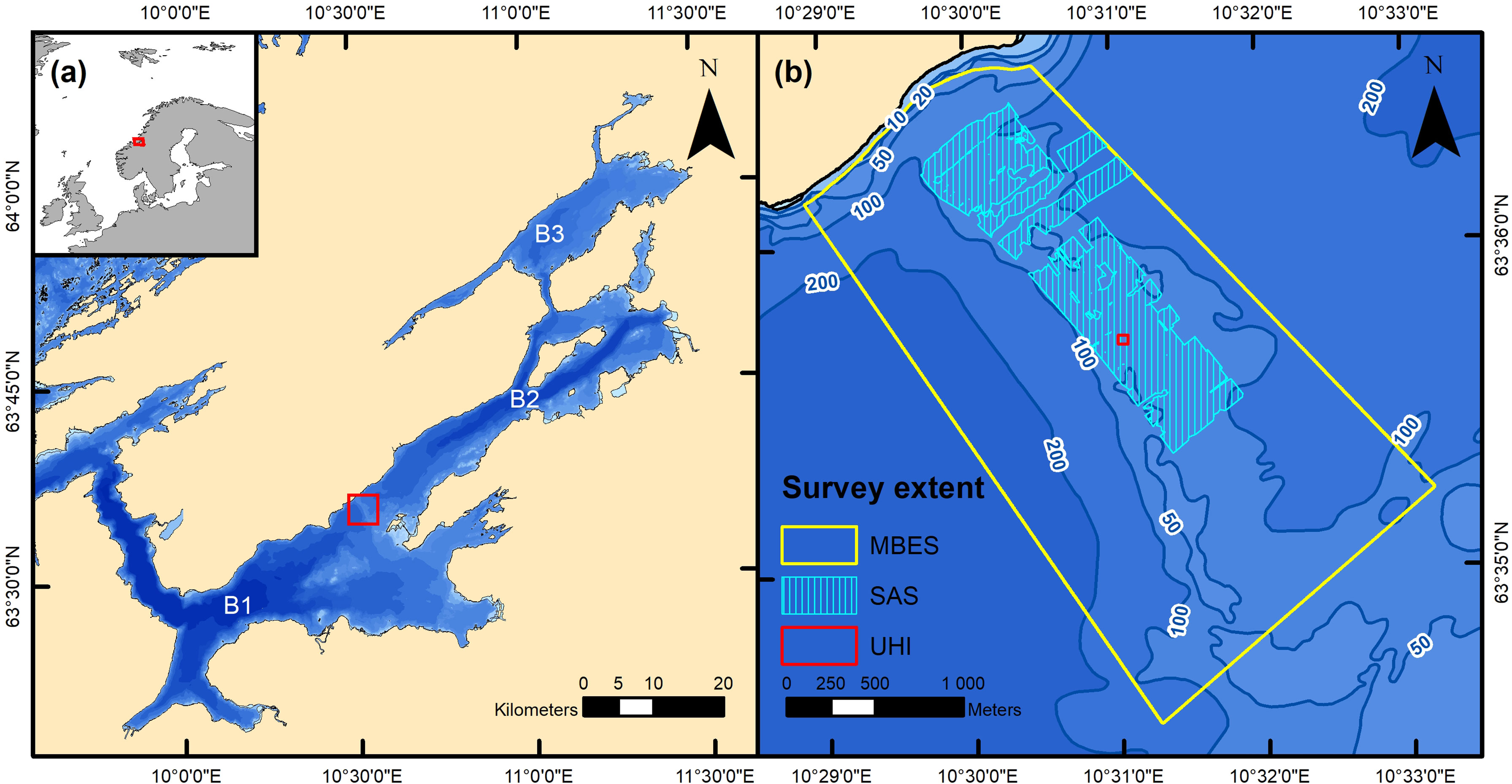
Figure 1 The area surveyed in the current study. Panel (A) shows a map of the Trondheimsfjord with the fjord’s geographic position indicated in the upper left corner. B1, B2 and B3 correspond to the fjord’s outer, middle and inner basin, respectively. The red square indicates the position of the Tautra Ridge and the extent of panel (B). Panel (B) shows a depth contour map of the most pronounced part of the Tautra Ridge (depths are given in meters) and the spatial extent of the datasets utilized in the study. The data were obtained using three different techniques: multibeam echo sounding (MBES), synthetic aperture sonar (SAS) imaging and underwater hyperspectral imaging (UHI). The maps were created in ArcMap (v. 10.8; Esri Inc., Redlands, USA; https://desktop.arcgis.com/en/arcmap/). The depth contour maps are based on data from the Norwegian Mapping Authority (Kartverket), available at https://kartkatalog.geonorge.no/Metadata/dybdedata/2751aacf-5472-4850-a208-3532a51c529a under CC BY 4.0 license. Projection: UTM 32N. Datum: WGS 1984.
Extending from 63°36’30”N 10°30’E to 63°34’N 10°35’E, the ~6-km Tautra Ridge supports some of the world’s shallowest cold-water coral (CWC) reefs (39 m; Brooke and Järnegren, 2013). A reef is here defined as a biogenic framework consisting of both living and dead coral. Radiocarbon labelling suggests that the Tautra Ridge was formed 10,800-10,500 14C years BP (Reite, 1995; Lyså et al., 2008), and with depths generally ranging from 39 to 100 m, it spans the full width of the Trondheimsfjord (Figure 1B). The CWCs associated with the Tautra Ridge do not form a continuous reef structure, but rather a complex of discrete, adjacent CWC build-ups ranging from 10 to 105 m2 in size (Mortensen and Fosså, 2001). The currents across the ridge are influenced by season, tide and local bathymetry, but can invariably be considered strong. At 80-m depth, eastward currents with speeds up to 0.7 m s-1 have for instance been recorded (Jacobson, 1983). Over the past decades, the biological value of the Tautra Ridge has become increasingly acknowledged by the Norwegian Government, and in 2013, the ridge was named one of Norway’s first marine protected areas (MPAs; Lovdata, 2013).
The species that dominates the Tautra CWC reef complex is the scleractinian coral Desmophyllum pertusum (Linnaeus, 1758), formerly known as Lophelia pertusa. Desmophyllum pertusum is a cosmopolitan coral species that so far has proven to be particularly abundant in the North Atlantic and its associated fjord systems (Davies et al., 2008). Its known depth range spans all the way from 39 m at the Tautra Ridge to a maximum recorded depth of 3,383 m in the Northwest Atlantic (Squire, 1959). On the Norwegian continental shelf, D. pertusum is most common at 200-400-m depths, but in Norwegian fjords, it is frequently encountered in shallower waters (Mortensen et al., 1995; Fosså et al., 2002). On a general basis, D. pertusum can be considered relatively tolerant with respect to environmental variables (Järnegren and Kutti, 2014). In the Northeast Atlantic, it does, however, seem to prefer salinities close to 35, temperatures of 6-9°C and oxygen levels of 6.0-6.2 mL L-1 (Davies et al., 2008; Roberts et al., 2009), which coincides well with the environmental conditions at the Tautra Ridge.
Desmophyllum pertusum’s ability to create complex, three-dimensional reef structures makes it an important ecosystem engineer in cold waters (Jones et al., 1994; Mortensen et al., 2010). Despite its slow growth rate (typically <1 cm year-1; Sabatier et al., 2012), the species is capable of forming vast bioherms, and the biggest D. pertusum reef complex known to date is the ~40 km long Røst Reef off the coast of northern Norway (Fosså et al., 2005). As a structure-forming ecosystem engineer, D. pertusum provides substrate and shelter to a range of benthic and demersal organisms. In the Northeast Atlantic as a whole, it is known to co-occur with >1,300 species (Roberts et al., 2006), and at the Tautra Ridge, >120 macrofaunal species have so far been documented (Mortensen and Fosså, 2001; Costello et al., 2005; Mortensen and Fosså, 2006). Historically, published studies of the Tautra CWC reef complex have relied heavily on physical point sampling. However, there also exist non-invasive methods of obtaining coral information that hitherto have remained relatively unexplored in the current study area.
Desmophyllum pertusum’s eco-geographical preferences and morphological properties make the Tautra CWC reef complex an interesting target for acoustic remote sensing surveys. From a geomorphometric perspective, D. pertusum in the Northeast Atlantic is for instance known to be associated with bathymetric highs, steep slopes and irregular seafloor surfaces (Mortensen et al., 2001; Davies et al., 2008; Davies et al., 2017), all of which are seafloor variables that can be quantified using, e.g., multibeam echo sounding (MBES; Wilson et al., 2007). Furthermore, the corals themselves may on multiple levels serve as suitable targets for acoustic detection. Firstly, being a scleractinian coral species, D. pertusum deposits calcium carbonate in the form of aragonite in order to grow. In Norwegian waters, the solid aragonite skeletons of dense D. pertusum frameworks have been shown to produce stronger MBES backscatter than, e.g., soft-bottom sediments, which may provide a partial means of reef identification (Fosså et al., 2005). It should, however, be noted that this is not necessarily thought to be the case if the corals grow in less dense frameworks. Secondly, vertical coral growth may generate abrupt angles between the reef perimeter and the surrounding seafloor. This is an attribute that can be identified by side-scanning sonar systems, which produce imagery where protruding seafloor features typically display strong acoustic backscatter and cast distinctive acoustic shadows (Fosså et al., 1997; Blondel, 2009). Finally, and perhaps most importantly, D. pertusum’s complex three-dimensionality potentially gives its reefs characteristic acoustic signatures in sonar imagery. In Norwegian waters, D. pertusum often has a tightly branching and hemispherical growth pattern, which typically is manifested as noisy, rough-textured areas, sometimes referred to as “cauliflower patterns” (Freiwald et al., 2002; Fosså et al., 2005; De Clippele et al., 2018). In 2012, the Tautra Ridge was acoustically surveyed using a HUGIN 1000 autonomous underwater vehicle (AUV) from Kongsberg Maritime AS (Kongsberg, Norway). The HUGIN AUV was equipped with a synthetic aperture sonar (SAS), and the recorded sonar imagery clearly revealed the presence of cauliflower-patterned reef structures (Ludvigsen et al., 2014). Sture et al. (2018) later demonstrated that these D. pertusum reefs could be accurately identified in SAS imagery by applying a convolutional neural network (CNN) classification algorithm.
The morphological properties of D. pertusum also permit reef detection by means of optical remote sensing. Most notably, D. pertusum is known to have two distinct color phenotypes: white and orange. Both phenotypes spectrally differ considerably from dead coral structures, which potentially may constitute >70% of the reef framework (Vad et al., 2017). The reason as to why the two phenotypes exist and grow side by side is currently a topic under investigation. What is known, is that the color difference as such likely is caused by carotenoid pigments, such as astaxanthin, which are more than twice as abundant in the orange phenotype (Elde et al., 2012). What is yet to be determined, is the exact mechanism behind the difference in carotenoid contents. One of the leading hypotheses is currently that the coloration is linked to the bacterial composition of the D. pertusum mucus layer, which further is thought to influence the coral’s nutritional uptake (Neulinger et al., 2008; Provan et al., 2016). From a physiological perspective, the difference between the two phenotypes is also unclear, but findings from a recent study by Büscher et al. (2019) suggest that the orange phenotype may be more resistant to stress than its white counterpart. At present, only a few published studies feature optical survey results from the Tautra CWC reef complex. In September 2000, the northwestern part of the Tautra Ridge was optically investigated using a remotely operated vehicle (ROV) equipped with two video cameras (Mortensen and Fosså, 2001). The survey was performed by the Norwegian Institute of Marine Research and aimed to map D. pertusum occurrences and associated biodiversity. In total, ~6,200 m of video transect were analyzed, and the documented biodiversity was found to be greater than that of equivalent seafloor areas on the Norwegian continental shelf. In 2012, a small area (200-300 m2) of the Tautra Ridge was surveyed in detail using an ROV equipped with two video cameras, a downward-facing digital camera and an underwater hyperspectral imager (Ludvigsen et al., 2014; Johnsen et al., 2016). During the survey, D. pertusum was optically confirmed to be present, but the resulting data were not analyzed extensively. More recently, ROV-acquired video from the Tautra Ridge was used to verify coral presence in acoustic SAS imagery (Sture et al., 2018). Here, the optical information served as a useful qualitative guide, but the video data were not assessed quantitatively.
Over the past decade, the Norwegian University of Science and Technology (NTNU) has collected both acoustic and optical remote sensing datasets from the Tautra Ridge and its associated D. pertusum reefs. However, very little of this material has to date been published in a geospatial context. The aim of the current study was therefore to synthesize available data to provide enhanced insight into the frequently referenced but poorly documented Tautra CWC reef complex.
The study utilized data from three major remote sensing techniques: (1) ship-based MBES, (2) AUV-based SAS imaging and (3) ROV-based underwater hyperspectral imaging (UHI; Figure 1B). Data from the first of these techniques were used to estimate seven geomorphometric seafloor variables covering most of the Tautra Ridge, whereas data from the latter two techniques were used to outline and characterize D. pertusum occurrences at two different spatial scales. Ultimately, geomorphometric variable values from areas with and without corals present were compared, and an attempt was made to predict CWC reef distribution along the ridge. Figure 2 shows a flowchart that outlines the steps presented in the Materials and Methods section.
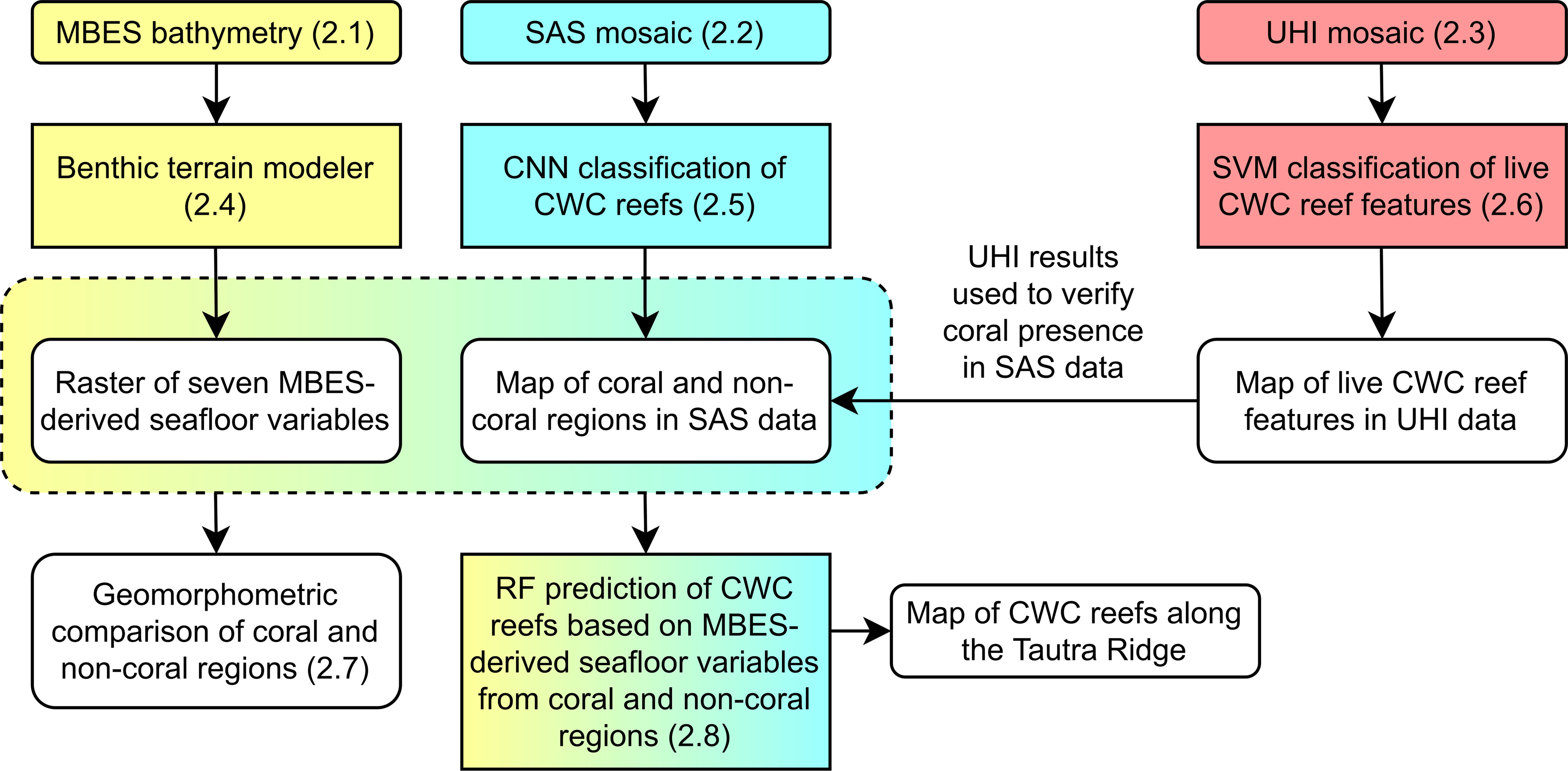
Figure 2 Flowchart of the steps presented in the Materials and Methods Section (sections 2.1-2.8). CNN, convolutional neural network; CWC, cold-water coral; MBES, multibeam echo sounding; SAS, synthetic aperture sonar; SVM, support-vector machine; UHI, underwater hyperspectral imaging.
2 Materials and Methods
2.1 MBES Data
In April 2016, a georeferenced MBES point cloud from the most pronounced part of the Tautra Ridge was obtained from the Norwegian Mapping Authority’s Hydrographic Service (Kartverket Sjødivisjonen, Stavanger, Norway). The point cloud had been collected using a Kongsberg EM 710 MBES system (Kongsberg Maritime AS, Kongsberg, Norway) onboard the survey vessel MS Hydrograf. The data were initially classified, but approved for release to NTNU’s Applied Underwater Robotics Laboratory (AURLab) for the purpose of research and education. The released MBES data featured detailed bathymetric information but did not contain information on acoustic backscatter intensity. Based on the MBES point cloud, a gridded bathymetric dataset with a spatial resolution of 2 m x 2 m was generated. This dataset covered an area of 6.23 km2 and served as the basis for all geomorphometric analyses presented herein.
2.2 SAS Data
The SAS data utilized in the current study were collected in December 2012 during a joint research cruise arranged by NTNU’s AURLab and the Norwegian Defense Research Establishment (FFI, Kjeller, Norway). To record sonar imagery, a Kongsberg HiSAS 1030 synthetic aperture sonar system (Kongsberg Maritime AS, Kongsberg, Norway) was deployed on a HUGIN 1000 AUV. As opposed to regular side-scanning sonar systems, SAS systems utilize more than a single ping to reconstruct a given location in the output imagery, which improves spatial resolution both across- and along-track (Hansen et al., 2004; Sture et al., 2018). Using the SAS-equipped HUGIN AUV, the northwestern region of the Tautra Ridge was surveyed in a systematic lawnmower pattern at a mean seafloor altitude of 26 m. The resulting imagery was post-processed in Kongsberg Maritime’s “Reflection” software, and ultimately georeferenced at a pixel resolution of 4 cm x 4 cm. The final SAS mosaic covered a seafloor area of ~1 km2.
2.3 UHI Data
A Tautra Ridge CWC reef situated at 80-m depth at approximately 63°35’43”N 10°31’3”E was optically surveyed by NTNU’s AURLab in March 2017. The survey utilized a SUB-fighter 30k ROV (Sperre AS, Notodden, Norway) equipped with a 4th generation underwater hyperspectral imager (UHI-4) from Ecotone AS (Trondheim, Norway). UHI-4 is an optical imager that contains two cameras: (1) a regular digital camera (red, green, blue; RGB) and (2) a hyperspectral push-broom scanner capable of recording imagery where each pixel holds a contiguous light spectrum as opposed to an RGB value. The high spectral resolution of the technique potentially provides an enhanced data foundation with potential for the identification of spectral signatures (“fingerprints”) that may be useful for automated mapping of seafloor features based on color. Being a push-broom scanner, the latter camera operates by capturing hyperspectral pixel rows through a narrow light entrance slit at a fixed frame rate. To provide spatially coherent hyperspectral imagery, UHI-4 must therefore be maneuvered in straight lines across the given area of interest, with the light entrance slit of the hyperspectral camera oriented perpendicularly to the instrument platform’s heading. Over the past decade, UHI-based seafloor studies have been carried out within a variety of fields (e.g., marine biology and archaeology), and for an overview of the technique, see Liu et al. (2020) and Montes-Herrera et al. (2021).
For the current study’s optical survey, UHI-4 was mounted on the SUB-fighter 30k ROV in a nadir viewing position, with two downward-facing 250-W Deep Multi SeaLite halogen lamps (DeepSea Power & Light LLC, San Diego, USA) placed 35 cm port and starboard of the instrument. The ROV was subsequently deployed at the survey location, using NTNU’s research vessel, RV Gunnerus. To provide geospatial context to the data acquisition, the ROV utilized a dynamic positioning system (Sørensen et al., 2012) and a navigation filter aided by an acoustic ultra-short baseline (USBL) positioning system mounted on the surface vessel. This permitted the ROV to follow a pre-programmed lawnmower pattern at a seafloor altitude of 2 m. The pattern consisted of 13 parallel, partially overlapping transects and covered a reef area of approximately 800 m2. While following the pattern, UHI-4 captured optical imagery according to the settings specified in Table 1.
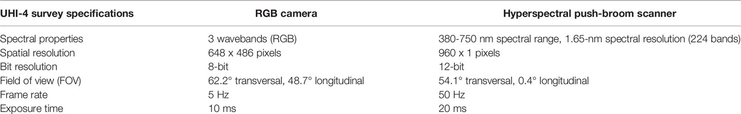
Table 1 UHI-4 specifications relevant for the 2017 cold-water coral (CWC) survey on the Tautra Ridge.
Following the optical data acquisition, the imagery was processed in a succession of steps, according to the procedure described in Løvås et al. (2021). First, the acquired RGB imagery (a total of 21,702 images) was used to generate a three-dimensional (3D) model of the survey area in the photogrammetry software Agisoft Metashape Professional (v. 1.6.2; Agisoft LLC, St. Petersburg, Russia). This model provided highly detailed estimates of UHI-4’s position (northing, easting and depth) and orientation (pitch, roll and yaw) over the course of the survey. Using these estimates, the underwater hyperspectral imagery was subsequently ray-casted onto the 3D model according to the hyperspectral push-broom scanner’s known geometric model relative to the RGB camera. By estimating the geographic intersections between the 3D model and the push-broom scanner’s field of view (FOV), the hyperspectral imagery was georeferenced on a pixel-specific basis at a spatial resolution of 1 cm x 1 cm. Ultimately, the georeferenced UHI data were converted from spectral radiance (L(λ)) to spectral reflectance (R(λ)) using Beer-Lambert’s law for non-scattering media modified from Mobley (1994). The final UHI mosaic covered an area of ~787 m2 (see Supplementary Figure S1).
2.4 Estimation of Geomorphometric MBES Variables
The MBES-derived depth data from the Tautra Ridge were analyzed in the geospatial processing software ArcMap (v. 10.8; Esri Inc., Redlands, USA) using the Benthic Terrain Modeler (BTM) 3.0 plug-in (Walbridge et al., 2018). In addition to depth, six geomorphometric variables were estimated: broad bathymetric position index (BPI broad), fine bathymetric position index (BPI fine), slope, ruggedness, eastness and northness. While depth corresponds to a grid cell’s vertical position relative to the sea surface, BPIs are calculated based on neighborhood analyses and indicate a grid cell’s bathymetric position relative to its surroundings. The exact value range of a BPI will depend on the dataset as well as the chosen analysis settings. Positive and negative values respectively denote bathymetric highs (e.g., ridges and mounds) and lows (e.g., valleys and troughs), whereas values close to 0 represent flat or constantly sloping seafloor areas (Weiss, 2001). As a rule, finer-scale BPIs (smaller neighborhood sizes) are potentially capable of picking up smaller bathymetric features of interest. In the current study, the broad- and fine-scale BPIs were standardized according to Weiss (2001). The slope variable indicates the maximum rate of bathymetric change between a grid cell and its neighbors. Slope is typically given in degrees (°), and possible values range from 0 (flat areas) to 90 (vertical drops). Ruggedness can be characterized as the degree of three-dimensional variation within a grid cell neighborhood. It is calculated based on dispersion of orthogonal grid cell vectors within the given neighborhood, and possible values range from 0 (completely homogeneous surface) to 1 (completely heterogeneous surface). Finally, the variables eastness and northness both relate to the aspect (direction) of a grid cell’s downslope. Possible values for the two variables range from -1 to 1, where -1 denotes an entirely westward (eastness) or southward (northness) downslope direction and 1 denotes an entirely eastward (eastness) or northward (northness) downslope direction. The settings used to derive the geomorphometric variables in the BTM 3.0 ArcMap plug-in are listed in Table 2.
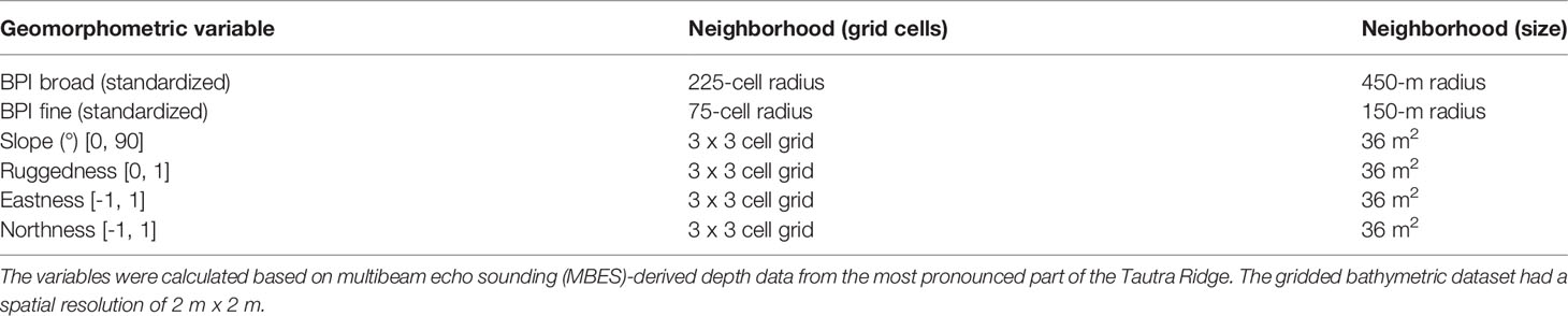
Table 2 Settings used to estimate six geomorphometric variables in the Benthic Terrain Modeler (BTM) 3.0 ArcMap plug-in.
2.5 Estimation of CWC Reef Distribution in SAS Imagery
CWC reef distribution in the full Tautra Ridge SAS mosaic from 2012 was estimated using a CNN classifier. In recent years, CNNs have grown to become powerful deep learning tools for classifying data that are structured in multiple arrays (e.g., two-dimensional imagery; LeCun et al., 2015). A CNN consists of a set of alternating convolution and pooling layers. During training, each kernel-based convolution layer generates a set of unique feature maps, which subsequently are downsampled in a pooling layer to reduce computational time in the next round of convolutions. Ultimately, all feature maps and their neural couplings are assembled to one or more fully connected layers capable of recognizing patterns based on the utilized training data. When new data are provided to a pre-trained CNN classifier, the output is typically a vector or matrix of probabilistic values corresponding to the input data’s likelihood of belonging to different classes.
The CNN classifier used in the current study was implemented in TensorFlow Keras (Abadi et al., 2016). Structurally, the CNN consisted of four blocks of convolution/pooling, followed by two fully connected layers. The classifier was trained on a selection of SAS image subsets (100 x 100 pixels) from three different HUGIN AUV deployments. All training data had a spatial pixel resolution of 4 cm x 4 cm, and the total CNN training set consisted of >30,000 images distributed among two classes: images with D. pertusum present and images with D. pertusum absent. Of the full training set, 20% of the images were set aside for model validation, and for the final classification model, an accuracy of 95% was reported. For further details on the development and training of the CNN, see Sture et al. (2018).
Applying the pre-trained CNN to the full Tautra Ridge SAS mosaic yielded a CWC reef distribution map with a spatial resolution of 80 cm x 80 cm, where each grid cell contained a georeferenced probability (0-1) of coral presence. These probabilities were subsequently labeled into three discrete classes: the coral class (grid cells with a probability of coral presence >0.99), the control class (grid cells with a probability of coral presence <0.50) and the intermediate class (all remaining grid cells). The thresholds used to define the classes were chosen subjectively based on their perceived ability to accurately isolate coral regions (the coral class) from non-coral regions (the control class). The seafloor regions outlined by the coral class and the control class later provided the basis for the assessment of geomorphometric trends related to D. pertusum coverage on the Tautra Ridge.
2.6 Estimation of Live CWC Reef Coverage in Underwater Hyperspectral Imagery
To estimate live CWC reef coverage in the UHI survey area, the underwater hyperspectral imagery was analyzed using support-vector machine (SVM) classification with a radial basis function (RBF) kernel. The SVM algorithm uses vector-defined decision surfaces to maximize the margins between the provided training set classes and is known to be well-suited for high-dimensional datasets (Cortes and Vapnik, 1995; Mountrakis et al., 2011). It has also performed favorably in previous seafloor mapping studies featuring UHI (Chennu et al., 2017; Dumke et al., 2018; Mogstad et al., 2020). During the optical CWC survey in March 2017, the live fraction of the present CWC reef framework was observed to primarily consist of white D. pertusum, orange D. pertusum and the sponge Mycale cf. lingua (Bowerbank, 1866). The spectral signatures of these species were consequently chosen as supervised classification targets.
For the SVM classification, the georeferenced UHI mosaic was spectrally subset to the range of 400-650 nm and binned down to a spectral resolution of 3.3 nm, resulting in a total of 75 color bands (wavelengths). This was done to remove wavelengths with low signal-to-noise ratio and to make the ensuing spectral classification computationally less intensive. SVM training data were subsequently obtained from pixel regions of the UHI mosaic corresponding to white D. pertusum, orange D. pertusum and Mycale cf. lingua. The total training set consisted of 2,400 pixels, evenly distributed among the three spectral targets (the R(λ) signatures of the different targets are shown in Supplementary Figure S2). By performing a ten-fold cross-validation on the selected training data in the statistical software environment R (v. 4.0.2; R Foundation for Statistical Computing, Vienna, Austria) using the package “e1071” (Meyer et al., 2020), the optimal values for RBF-SVM parameters γ (kernel width) and C (degree of regularization) were in the current study found to be 1e-05 and 1e06, respectively (cross-validation accuracy = 100%). Using these parameter values, the SVM classification algorithm was ultimately applied to the full UHI mosaic in the software application ENVI (Environment for Visualizing Images, v. 5.6; Harris Geospatial Solutions Inc., Broomfield, USA). The full classification was performed with a probability threshold of 0.95, implying that only pixels with probabilities of belonging to a training set class beyond 0.95 were classified.
2.7 Geomorphometric Comparison of Coral and Non-Coral Regions
For the geomorphometric comparison of coral and non-coral regions, all MBES-derived seafloor variables (depth, BPI broad, BPI fine, slope, ruggedness, eastness and northness) were combined into a single 7-band raster. From the combined raster, values from grid cells covered entirely by either the coral class or the control class of the classified CNN coral distribution map were subsequently extracted for analysis. The extracted dataset consisted of 24,388 coral cells and 122,963 control cells (each cell corresponding to a 2 m x 2 m area). For each MBES-derived variable, the median and interquartile range was calculated for both classes, and a two-sided Mann-Whitney rank sum test was performed to investigate whether coral regions differed significantly from control regions.
2.8 Geomorphometric CWC Reef Classification
To assess the feasibility of CWC reef identification by means of geomorphometry alone, the dataset extracted in Geomorphometric Comparison of Coral and Non-Coral Regions was also used to generate a random forest (RF) prediction model. An RF is an assemblage of decision trees created from randomly selected subsets (bootstrapped samples) of the provided training data (Breiman, 2001). For classification purposes, RF training data are typically composed of one categorical response variable (class) and a set of corresponding explanatory variables (predictors). When an unclassified sample is provided to a pre-trained RF prediction model, all decision trees individually vote for the most likely class based on the values of the provided predictors. These votes are subsequently pooled together, and the final output from the RF algorithm is the class that obtained the majority vote (the dichotomization may alternatively be decided by a user-defined probability cutoff). In the current study, the RF algorithm was chosen due to its ability to handle complex interactions, correlated predictors and irregular variable distributions (Cutler et al., 2007). In addition, the RF algorithm has yielded promising results in previous attempts to classify CWC reef structures in MBES-derived data (De Clippele et al., 2017; Diesing and Thorsnes, 2018).
For the RF classification, the extracted data were randomly partitioned into a training set (80% of the samples), a validation set (10% of the samples) and a test set (10% of the samples). The ratio of coral samples to control samples was equal in all partitions (approximately 1:5). The RF prediction model was developed in the statistical software environment R using the package “randomForest” (Liaw and Wiener, 2002). RF modeling requires specification of two parameters: the number of decision trees to grow (ntree) and the number of features (predictor variables) to consider during each split (mtry). These parameters were optimized using ten-fold cross-validation, which revealed that ntree = 1000 and mtry = 5 yielded the best tradeoff between accuracy (out-of-bag error rate = 0.08) and processing time. By subsequently maximizing the model’s overall classification accuracy (OCA) based on the validation set, the optimal probability cutoff for differentiating coral samples from control samples was found to be 0.42 (i.e., samples receiving >42% of the decision tree votes in favor of the coral class were considered to be coral). The final RF prediction model was applied to the test set, and the results were evaluated with respect to the performance metrics listed in Table 3.
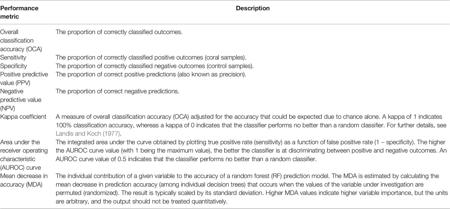
Table 3 Descriptions of performance metrics used to evaluate the random forest (RF) prediction model.
Ultimately, CWC reef distribution was estimated along the Tautra Ridge by applying the RF prediction model to all regions of the full 7-band MBES raster that contained variable values inside the range of the RF training set (amounting to 4.55 km2 of the full raster; regions with variable values exceeding the training set were omitted because RF predictions are known to be unreliable for samples outside the modeled range). For this classification, the results were dichotomized at three different probability cutoffs: maximized validation set OCA (probability cutoff = 0.42), validation set negative predictive value (NPV) = 0.95 (probability cutoff = 0.39) and validation set positive predictive value (PPV) = 0.95 (probability cutoff = 0.72). The former cutoff was chosen to provide a CWC reef coverage estimate with optimized accuracy. The latter two cutoffs were chosen to provide realistic upper and lower boundaries to the optimized estimate. The rationale behind choosing 0.39 as the upper boundary, was that at NPV = 0.95, at least 95% of the negative (control) predictions could be expected to be correct. Similarly, the rationale behind choosing 0.72 as the lower boundary, was that at PPV = 0.95, at least 95% of the positive (coral) predictions could be expected to be correct.
3 Results
3.1 MBES and SAS Results
Figure 3A shows the MBES-derived bathymetric map used to acquire geomorphometric information from the Tautra Ridge. The structure of the ridge was evident in the map, with the ridge crest oriented perpendicularly to the fjord’s direction (see Figures 1, 3A) and notable downward slopes towards the southwest and northeast. Geographic heatmaps of the variables BPI broad, BPI fine, slope, ruggedness, eastness and northness are shown in Supplementary Figure S3.
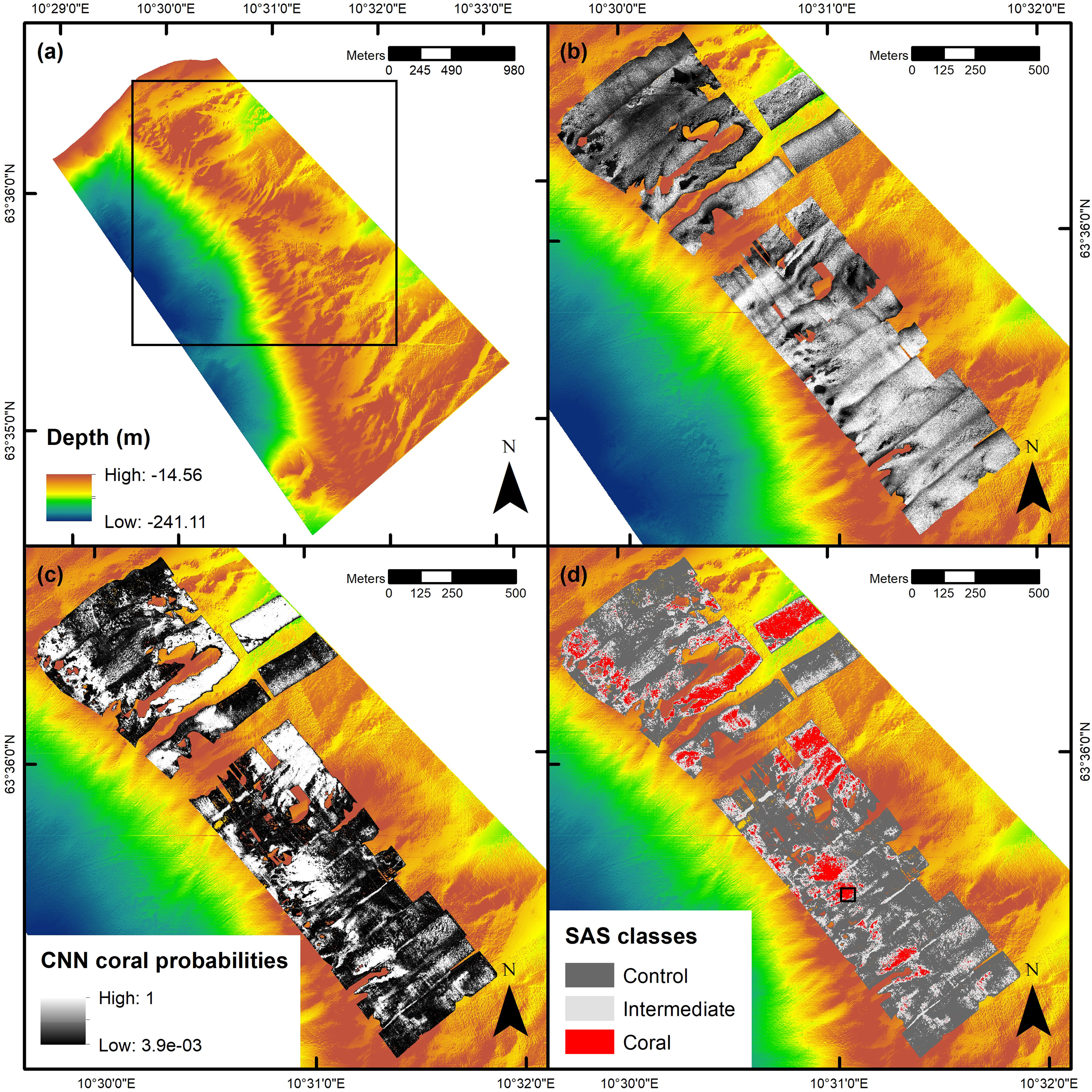
Figure 3 Multibeam echo sounding (MBES) and synthetic aperture sonar (SAS) imaging results. Panel (A) shows the MBES-derived bathymetric map of the most pronounced part of the Tautra Ridge (declassified bathymetry, map courtesy of the Norwegian Mapping Authority). The black square indicates the spatial extent of panels (B-D). Panel (B) shows the Tautra Ridge SAS mosaic. Panel (C) shows the georeferenced probabilities of coral presence obtained from the convolutional neural network (CNN). Panel (D) shows the classified coral distribution map generated based on the probabilities in panel (C) and the thresholds defined in Estimation of CWC Reef Distribution in SAS Imagery. The black square indicates the position of the underwater hyperspectral imaging (UHI) mosaic presented in Figure 4. The maps were created in ArcMap (v. 10.8; Esri Inc., Redlands, USA; https://desktop.arcgis.com/en/arcmap/). Projection: UTM 32N. Datum: WGS 1984.
The AUV-acquired SAS dataset covered ~1 km2 of the 6.23 km2 MBES-surveyed area (Figure 3B), and acoustic cauliflower patterns assumed to correspond to reef structures were interspersed throughout the SAS survey area (an example is shown in Supplementary Figure S4). Based on the results of the CNN prediction model (Figure 3C) and the classification thresholds defined in Estimation of CWC Reef Distribution in SAS Imagery, CWC reefs (the coral class) were estimated to cover 0.12 km2 of the SAS-surveyed area, whereas non-coral regions (the control class) were estimated to cover 0.63 km2 (Figure 3D). The intermediate class covered the remaining 0.25 km2.
3.2 UHI Results
Overall, the UHI results agreed well with the acoustic findings from the SAS analysis. The georeferenced UHI mosaic covered an area of 786.7 m2, and 661.5 m2 of this area corresponded to regions acoustically identified as coral by the CNN classifier (Figure 4A). Based on the hyperspectral SVM classification (Figure 4B), live reef structures (i.e., white D. pertusum, orange D. pertusum and the sponge Mycale cf. lingua) were estimated to cover 15.5% of the total UHI survey area and 17.3% of the UHI survey area identified as coral acoustically (Table 4). Within the surveyed area, white D. pertusum was estimated to be considerably more abundant than both orange D. pertusum and sponges (Table 4).
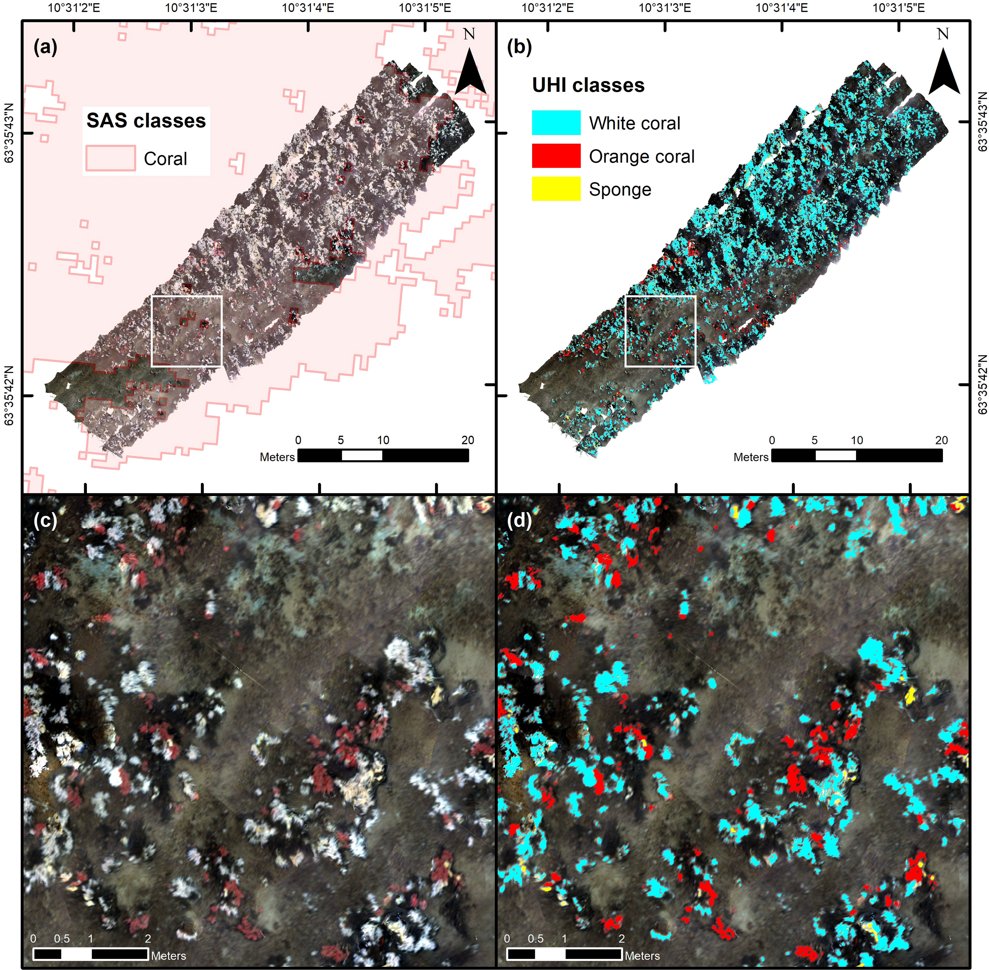
Figure 4 Underwater hyperspectral imaging (UHI) results. Panel (A) shows the georeferenced UHI mosaic visualized in red (R; 590 nm), green (G; 530 nm) and blue (B; 460 nm). Regions in the synthetic aperture sonar (SAS) imagery classified as “coral” by the convolutional neural network (CNN) classifier (see Estimation of CWC Reef Distribution in SAS Imagery) are highlighted in pink for comparison. Panel (B) shows the results of the hyperspectral support-vector machine (SVM) classification of UHI classes corresponding to live reef structures. Panels (C, D) show the areas indicated by white squares in panels (A, B), respectively. The maps were created in ArcMap (v. 10.8; Esri Inc., Redlands, USA; https://desktop.arcgis.com/en/arcmap/). Projection: UTM 32N. Datum: WGS 1984.
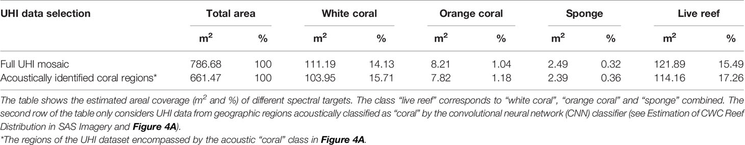
Table 4 Results of the support-vector machine (SVM) classification of the underwater hyperspectral imaging (UHI) dataset from the Tautra Ridge.
3.3 Geomorphometric Comparison of Coral and Non-Coral Regions
Probability densities of the geomorphometric variable values extracted from coral and control regions on the Tautra Ridge are shown in Figure 5. For all MBES-derived variables, the distribution differed significantly between the two classes (Table 5). Furthermore, for all but one of the variables (BPI broad being the exception), slightly elevated values were associated with the coral class. For the exception – BPI broad – the coral class displayed the highest median value, but the lowest overall value distribution (Figure 5B). The magnitude of the observed class difference varied between variables, and the most significant class discrepancies were observed for depth, slope, ruggedness and eastness (Table 5).
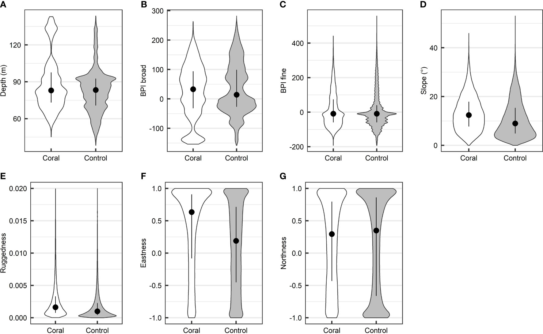
Figure 5 Geomorphometric comparison of coral (n = 24,388 grid cells) and non-coral (control; n = 122,963 grid cells) regions on the Tautra Ridge. The data were obtained from areas classified as “coral” and “control” by the convolutional neural network (CNN) classifier (see Estimation of CWC Reef Distribution in SAS Imagery). The figure shows the class-specific median, interquartile range and probability density of seven multibeam echo sounding (MBES)-derived seafloor variables.
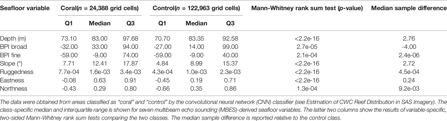
Table 5 Geomorphometric comparison of coral and non-coral (control) regions on the Tautra Ridge.
3.4 Geomorphometric CWC Reef Classification
The test set performance of the RF prediction model is summarized in the Table 6 confusion matrix. In total, the model performed well, with an OCA of 0.92 and an area under the receiver operating characteristic (AUROC) curve value of 0.95 (Figure 6A). Moreover, the obtained kappa coefficient of 0.71 indicated substantial agreement between predictions and true sample identities (Landis and Koch, 1977). However, the model was not without imperfections, and based on the observed sensitivity, specificity, PPV and NPV (Table 6), the model appeared to display a slight tendency towards underestimating coral abundance.
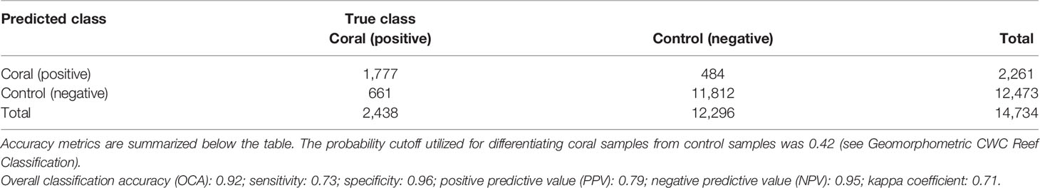
Table 6 Confusion matrix displaying the test set performance of the random forest (RF) prediction model.
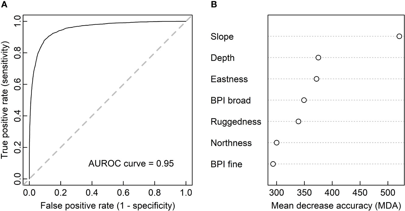
Figure 6 Results of the random forest (RF) coral classification. Panel (A) shows the prediction model’s area under the receiver operating characteristic (AUROC) curve for the test set. The dashed diagonal line symbolizes a hypothetical AUROC curve value of 0.5 (no ability to discriminate between coral and control samples). Panel (B) shows the RF prediction model’s mean decrease in accuracy (MDA; scaled by standard deviation) among decision trees when individual variables are randomized. Higher MDA values indicate higher variable contributions to the model’s performance.
In terms of individual predictor importance, the variable slope contributed the most to the prediction model’s accuracy (Figure 6B). In descending order, the variables depth, eastness, BPI broad and ruggedness made intermediate contributions, whereas northness and BPI fine contributed the least. The significance of these findings is further discussed in Geomorphometric CWC Coverage Trends.
Applying the RF prediction model to the 7-band MBES raster with the probability cutoffs defined in Figure 7A yielded the CWC reef coverage estimates displayed in Figure 7B and Table 7. The returned estimates ranged from 0.19 km2 to 0.72 km2, with the optimized OCA estimate suggesting a Tautra Ridge CWC reef coverage of 0.64 km2. Figure 8 shows a spatial representation of the RF classification results. Predicted CWC reef units were interspersed along the entire ridge, and within the regions surveyed by SAS and UHI, estimated coral coverage largely appeared to agree between the different remote sensing techniques (Supplementary Figure S4).
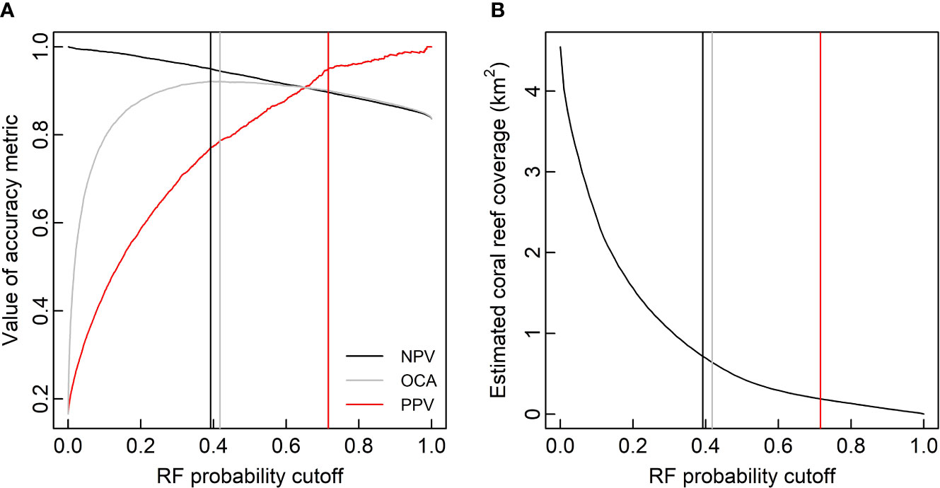
Figure 7 Cold-water coral (CWC) reef coverage along the Tautra Ridge estimated by the random forest (RF) prediction model at different probability cutoffs. Panel (A) shows the RF prediction model’s validation set negative predictive value (NPV), overall classification accuracy (OCA) and positive predictive value (PPV) plotted as functions of probability cutoff. The black, gray and red vertical lines respectively correspond to probability cutoffs where NPV = 0.95, OCA is maximized (0.92) and PPV = 0.95. Panel (B) shows estimated CWC reef coverage along the Tautra Ridge plotted as a function of RF probability cutoff. The vertical lines correspond to the three cutoffs defined in panel (A).
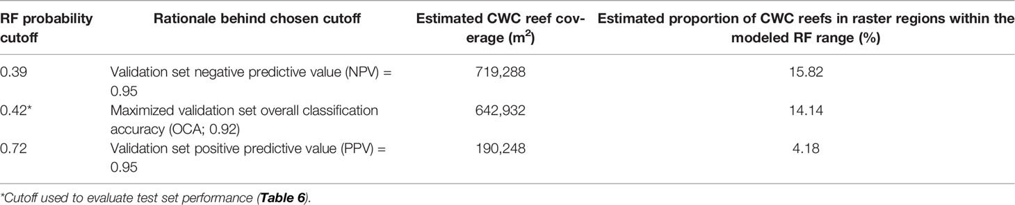
Table 7 Tautra Ridge cold-water coral (CWC) reef coverage estimated by the random forest (RF) prediction model at three different probability cutoffs.
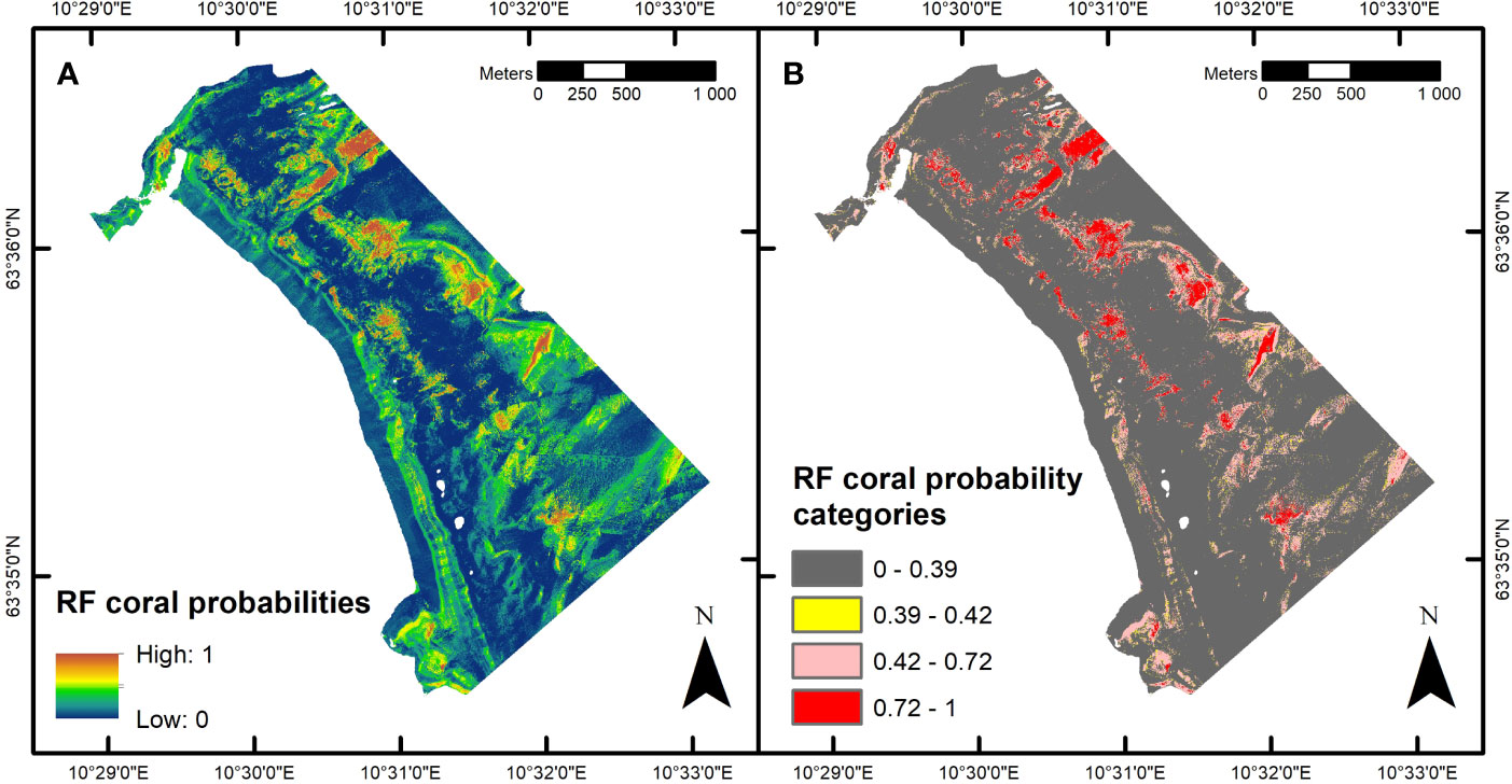
Figure 8 Estimated cold-water coral (CWC) reef distribution along the Tautra Ridge. Panel (A) shows floating point probabilities of coral presence estimated by the random forest (RF) prediction model. Panel (B) shows CWC reef distribution estimated at different probability cutoffs (see Geomorphometric CWC Reef Classification and Figure 7). The maps were generated in ArcMap (v. 10.8; Esri Inc., Redlands, USA; https://desktop.arcgis.com/en/arcmap/). Projection: UTM 32N. Datum: WGS 1984.
4 Discussion
4.1 Survey Techniques and Assumptions
The current study illustrated the value of applying multiple remote sensing techniques during the investigation and mapping of CWC reefs. At present, MBES systems (typically deployed on surface vessels) arguably represent the most efficient way of geospatially mapping ≥km-scale benthic habitats dominated by large biogenic structures. In previous CWC studies, MBES-derived data have for instance been used to address issues ranging from localized distribution of CWC reefs (Roberts et al., 2005; Guinan et al., 2009a; De Clippele et al., 2017; Diesing and Thorsnes, 2018) to D. pertusum habitat suitability along the entire Norwegian continental shelf (Sundahl et al., 2020). MBES also proved valuable in the current assessment of the Tautra Ridge, especially with respect to its superior capacity for areal coverage. To fully capitalize on its potential, a sufficiently extensive ground truth dataset was, however, a vital prerequisite. As shown in this study, the ground truthing requirements concerning MBES mapping of D. pertusum reefs could be fulfilled by combining AUV-based SAS imaging with an ROV-based UHI survey. These two ground truthing techniques represented incremental steps towards increased level of detail in the remote sensing pyramid of observation. In the first step, distinct acoustic patterns assumed to belong to D. pertusum permitted estimation of CWC reef coverage in a ~1-km2 subset of the MBES-surveyed area. In the second step, the identity of the acoustic patterns assumed to belong to D. pertusum was verified optically in an ~800-m2 area. This optical verification increased the confidence not only in the SAS classification accuracy, but also the georeferencing of the SAS dataset, which eventually were to guide the MBES-based CWC reef classification along the entire Tautra Ridge. In summary, all remote sensing techniques employed in the current study played complementary roles in the quest for holistic knowledge: ROV-based optical imaging provided data with unprecedented spatial resolution and ground truthing accuracy but was limited in terms of areal coverage; AUV-based sonar imaging could detect acoustically distinct biogenic structures in large areas but provided little information besides from the geographic extent of the targets of interest; ship-based MBES was limited with respect to spatial resolution but generated data that covered the entire area of interest and brought geomorphometric context to the identified targets. The potential value of using data from multiple sensors and platforms during marine exploration efforts is further elaborated in, e.g., the integrated mapping and monitoring approach proposed by Nilssen et al. (2015), and in the future, application of such approaches will likely become increasingly more important.
The validity of the presented Tautra Ridge findings rests on two principal assumptions. Firstly, it was assumed that the georeferencing of the different remote sensing datasets was consistent. As in any marine seafloor survey, minor geospatial discrepancies were expected, but upon inspection, the alignment of the MBES-, SAS- and UHI-acquired data was considered more than sufficient for the scope of the work. Supplementary Figure S4 exemplifies the observed positional coherence. Secondly, it was assumed that D. pertusum reef extent on the Tautra Ridge was unaltered between the acquisition of the first (December 2012) and the last (March 2017) dataset utilized in the study. It should be noted that this is an inherently erroneous assumption. However, considering D. pertusum’s slow growth rate (<1 cm year-1; Sabatier et al., 2012), and that the Tautra Ridge is an MPA where physical seafloor intervention is prohibited, it was nevertheless deemed reasonable for the analyses presented herein.
4.2 Optical CWC Coverage Trends
ROV-based UHI proved to be a valuable ground truthing technique for optical verification of acoustic CWC reef predictions. This is exemplified in Figure 4A and Supplementary Figure S4, where the CWC reef contours predicted by the acoustic CNN classifier closely match the coral distribution that can be observed in the recorded hyperspectral imagery. In addition to serving as a means of verifying reef presence, the optical UHI survey provided useful information on the survey area’s biological reef composition. Hyperspectral SVM classification for instance indicated that live D. pertusum and associated sponges covered ~17% of the regions in the survey area acoustically classified as coral (Table 4). Although this estimate only is based on spatially two-dimensional image analyses from a bird’s-eye view, it is exceptionally consistent with findings from a study by Vad et al. (2017), in which the ratio of live D. pertusum to whole colony size (i.e., both live and dead coral structures) ranged from 0.10 to 0.27, with a mean value of 0.17. The study by Vad et al. was carried out off the west coast of Scotland at relatively remote locations. If these locations are assumed to represent healthy CWC habitats and the estimated proportion of live coral (~17%) is used as a proxy for health, it can further be speculated that the Tautra Ridge CWC reef optically surveyed in the current study was in good condition. Regarding D. pertusum phenotype distribution, hyperspectral SVM classification revealed that the white D. pertusum phenotype was an order of magnitude more abundant than the orange phenotype within the UHI survey area (Figure 4B and Table 4). This trend is in accordance with observations from several other D. pertusum studies (Roberts, 2002; Larcom et al., 2014; Kellogg et al., 2017; Büscher et al., 2019), but its underlying cause remains to be determined. Overall, the UHI results showed that live D. pertusum easily could be mapped based on its spectral properties. One of the main benefits of applying UHI for the purpose of optical coral mapping was that live coral coverage accurately could be estimated using supervised classification (Figures 4C, D). Notably, the hyperspectral SVM classification only utilized a training set of 2,400 labeled pixels, which merely corresponded to 0.03% of the total UHI mosaic. This vastly increased data processing efficiency and firmly illustrated the value of employing automated approaches to optical seafloor mapping. In the future, we recommend conducting similar optical surveys at other CWC reefs on the Tautra Ridge. This will help substantiate the trends observed in the current study and improve our understanding of the Tautra CWC reef complex as a whole.
4.3 Geomorphometric CWC Coverage Trends
The comparison of coral and non-coral regions on the Tautra Ridge revealed that D. pertusum appeared to have certain preferences with respect to local geomorphometric seafloor variables. In the Mann-Whitney rank sum tests performed to compare coral-covered regions to their surroundings, the value distributions of all investigated variables were for instance found to significantly differ between the two seafloor classes (Table 5). However, some variables displayed more pronounced trends than others, and in terms of the observed probability densities, the variables slope and eastness stood out the most (Figures 5D, F). Specifically, the coral class was associated with steeper slopes (median = 12.41°; median sample difference = 2.72°) and more eastward-oriented terrain (median = 0.63; median sample difference = 0.24) than the control class. The former observation agrees well with findings from previous CWC studies from the Northeast Atlantic, which also suggest that D. pertusum prefers sloping terrain (Davies et al., 2008; Guinan et al., 2009b; Howell et al., 2011). The main reason for this preference is thought to be that slope-induced hydrodynamic phenomena (e.g., localized current patterns) may enhance the availability of suspended food particles (Frederiksen et al., 1992; Thiem et al., 2006; Davies et al., 2009). The interpretation of the latter observation is less clear-cut, as any preference with respect to aspect direction (in this case eastness) likely is linked to the directional dynamics of the surrounding currents. Being sessile suspension feeders, CWCs are often found to be associated with enhanced bottom currents (White and Dorschel, 2010). However, laboratory-based studies by Purser et al. (2010) and Orejas et al. (2016) suggest that excessive current velocities may impede D. pertusum’s food uptake. These findings are supported by a recent in situ study by Lim et al. (2020), in which current velocities ≥75 cm s-1 were found to restrict live D. pertusum coverage. Furthermore, at the Piddington Mound – a coral mound in the Porcupine Seabight exposed to current velocities of ~40 cm s-1 – live CWC reef framework was primarily found on the lee side of the mound (Lim et al., 2017). Interestingly, the interval of 40-75 cm s-1 coincides almost perfectly with the maximum bottom current speeds measured across the Tautra Ridge over the course of June 1974 (Jacobson, 1983). Since it also is known that the prevailing direction of these currents is eastward (Jacobson, 1983), a possible explanation for D. pertusum’s apparent inclination towards eastness on the Tautra Ridge (i.e., the lee side of the ridge) is therefore that it reduces current exposure to a level that facilitates the corals’ food uptake. To further investigate this hypothesis, we recommend deploying acoustic Doppler current profilers (ADCPs) at multiple locations on the Tautra Ridge over time, so that the spatiotemporal complexities of the in situ current patterns can be elucidated. In addition, routine surveys with ADCP-equipped AUVs along the ridge should be carried out, so that site-specific current measurements can be put into a broader spatial perspective.
Although less pronounced, some noteworthy coral coverage trends were also observed for the variables depth, BPI broad and ruggedness. Overall, the coral class was for instance found to be associated with slightly deeper waters and slightly lower BPI broad scores (Figures 5A, B and Table 5) than the control class. This initially seemed counterintuitive, as D. pertusum commonly is known to occur on bathymetric highs (Davies et al., 2008). However, these observations are, in fact, in accordance with the hypothesis stated in the previous paragraph: assuming the currents across the Tautra Ridge are strong enough to potentially impede D. pertusum’s food uptake or inflict unnecessary physical strain, it would be suboptimal for the corals to settle on the summit of the ridge. This could partially explain the observed patterns. It should be noted that the values of both depth and BPI broad displayed highly irregular probability densities, and their interpretation should consequently be treated with caution. Regarding ruggedness, the coral class was associated with significantly higher values than the control class (Table 5). This agrees with coarse-scale studies by Guinan et al. (2009b) and Davies et al. (2008), where D. pertusum also was found to be associated with irregular bathymetry. More importantly, it agrees with acoustic findings from a fine-scale CWC study by De Clippele et al. (2017), which was performed at a spatial resolution of 2 m. The reason for this tendency could be that bathymetric complexity is linked to increased access to suspended nutrition, reduced levels of sedimentation and/or a wider variability of substrate types (possibly favoring larval settling). However, at the high spatial resolution utilized in the current study (Table 2), the enhanced ruggedness could also be attributed to the three-dimensionality of the D. pertusum reef structures themselves. For instance, Price et al. (2019) and Price et al. (2021) recently utilized 3D models with sub-cm resolution to show that the structural complexity of CWC reefs often is considerably greater than that of surrounding non-reef regions. The least significant geomorphometric trends were observed for BPI fine and northness (Figures 5C, G and Table 5). For these variables, the coral class and the control class displayed highly similar median values and probability densities. This suggests that neither conveyed indispensable information with respect to CWC reef distribution in the current study.
4.4 Performance of the Geomorphometric CWC Reef Prediction Model
The RF model created to predict CWC reef coverage along the Tautra Ridge performed very well on the test set. As an example, all obtained accuracy metrics (Figure 6A and Table 6) were comparable to or exceeded those reported in similar studies by De Clippele et al. (2017) and Diesing and Thorsnes (2018). The RF probability cutoff that yielded the highest OCA resulted in a sensitivity of 0.73, a specificity of 0.96, a PPV of 0.79 and an NPV of 0.95. These results – specifically that sensitivity < PPV and specificity > NPV – indicate that the model was inclined to predict false negatives (type II errors) rather than false positives (type I errors). This may be interpreted as the model being conservative rather than exaggerated. The five predictors that contributed the most to the accuracy of the model were the variables slope, depth, eastness, BPI broad and ruggedness (Figure 6B). This was not surprising, considering that these were also the variables where the greatest differences between coral and non-coral regions had been observed previously (Figure 5 and Table 5). As the RF model applied in the current study only was based on seven geomorphometric variables derived from the same MBES dataset, its favorable performance can likely be attributed to the quality and size of the utilized training set. This emphasizes the importance of high-quality ground truthing, and attests to the value of applying multiple sensors and platforms in future studies of CWC reefs. Because the Tautra Ridge represents an unusual CWC habitat, it is unlikely that the utilized model can be directly applied to other locations. However, as the model was built and implemented in open-source software, the methodology can easily be adapted for other situations, provided that similar remote sensing data are available. An interesting future project would be to apply equivalent acoustic prediction models to CWC habitats where D. pertusum is known to form other reef frameworks than the dense cauliflower patterns present on the Tautra Ridge. Examples of such frameworks include fan-like growth patterns found in the Mediterranean Sea and columnar growth patterns found in the Gulf of Mexico and the Florida Straits (Sanna and Freiwald, 2021).
Although the RF prediction model performed favorably, inclusion of certain additional predictors could likely have enhanced its performance. Howell et al. (2011) for instance found substrate type to be highly important for predictive modeling of D. pertusum at coarser scales in the Northeast Atlantic. Similarly, Georgian et al. (2014) found that the availability of hard substrate was an important D. pertusum predictor in the Gulf of Mexico. In the current study, it is possible that acoustic backscatter intensity from MBES could have improved the coral prediction model by serving as a proxy for substrate type or capturing characteristic acoustic properties associated with coral presence (Fosså et al., 2005; Roberts et al., 2005). In addition to substrate, bottom current speed and direction have also proven to be useful variables in previous attempts to model CWC distribution (Davies et al., 2008; De Clippele et al., 2017; Sundahl et al., 2020). Unfortunately, sufficiently detailed data on the aforementioned variables were to our knowledge not available during the writing of this study. To increase the accuracy of future prediction models, it is therefore recommended that maps of substrate distribution, MBES backscatter intensity and current patterns on the Tautra Ridge are acquired.
5 Conclusions
The motivation behind the current study was to provide enhanced insight into the Tautra CWC reef complex, and based on the presented work, we believe the following can be presumed. Firstly, optical UHI analyses suggest that CWC reefs on the Tautra Ridge are dominated by the white D. pertusum phenotype. However, optical data were only acquired from a limited area, and further information is thus needed to support this claim. The underlying reason for the skewed phenotype distribution is also a topic that warrants further investigation. Secondly, acoustic analyses indicate that D. pertusum reef distribution on the Tautra Ridge is partially determined by bathymetric features. Specifically, relatively steep, eastward-sloping areas that are situated off the summit of the ridge appear to facilitate coral growth. The ultimate cause of this is likely linked to the patterns of the prevailing bottom currents, and further data on the surrounding hydrodynamic conditions can likely help elucidate the observed trends. Lastly, predictive modeling based on seafloor geomorphometry suggests that the following three conclusions can be drawn regarding D. pertusum reef extent on the Tautra Ridge: (1) D. pertusum reefs cover at least 0.19 km2 of the Tautra Ridge; (2) it is likely that D. pertusum reef extent on the Tautra Ridge is close to 0.64 km2; and (3) it is unlikely that D. pertusum reef extent on the Tautra Ridge currently exceeds 0.72 km2.
To our knowledge, this is the first attempt to characterize distribution and areal coverage of D. pertusum reefs on the Tautra Ridge extensively. Consequently, there are few data available to verify CWC reef predictions beyond the areas surveyed by SAS and UHI in the current study. Nevertheless, we believe the modeled estimates presented herein represent a valuable knowledge basis that decision-making authorities may refer to in efforts to govern the Tautra Ridge MPA sustainably. Furthermore, the results of this study may serve as a foundation for future research carried out in the area. Although D. pertusum is thought to be a relatively tolerant CWC species, its slow growth rate and high importance as an ecosystem engineer makes it a primary conservation target. In an era of climate change and increasing anthropogenic pressure, mapping and monitoring of such targets can arguably be considered more important than ever. In the future, it is therefore recommended that systematic ground truthing surveys are conducted along the entire Tautra Ridge so that the coral estimates presented in this study can be further refined. This will provide baseline information that should be considered essential not only for satisfactory MPA management, but also the continued existence of some of the world’s least conventional CWC reefs.
Data Availability Statement
The raw data supporting the conclusions of this article will be made available by the authors, without undue reservation.
Author Contributions
AM: developed the idea, participated in the data acquisition, performed data analysis and wrote the manuscript. HL and ØS: participated in the data acquisition, performed data analysis and provided textual input to the manuscript. GJ and ML: participated in the data acquisition and provided textual input to the manuscript. All authors contributed to the article and approved the submitted version.
Funding
This work has been carried out at the Centre for Autonomous Marine Operations and Systems (NTNU AMOS). This work was supported by the Research Council of Norway through the Centres of Excellence funding scheme (grant no. 223254 – NTNU AMOS).
Conflict of Interest
The authors declare that the research was conducted in the absence of any commercial or financial relationships that could be construed as a potential conflict of interest.
Publisher’s Note
All claims expressed in this article are solely those of the authors and do not necessarily represent those of their affiliated organizations, or those of the publisher, the editors and the reviewers. Any product that may be evaluated in this article, or claim that may be made by its manufacturer, is not guaranteed or endorsed by the publisher.
Acknowledgments
The authors would like to thank the Norwegian Mapping Authority’s Hydrographic Service for providing MBES data from the Tautra Ridge. The authors would also like to thank the Norwegian Defense Research Establishment, NTNU’s AURLab and the crew of RV Gunnerus for their valuable contributions concerning data collection and preparation.
Supplementary Material
The Supplementary Material for this article can be found online at: https://www.frontiersin.org/articles/10.3389/fmars.2022.848888/full#supplementary-material.
Supplementary Figure 1 | The georeferenced underwater hyperspectral imaging (UHI) mosaic from the Tautra Ridge visualized in red (R; 590 nm), green (G; 530 nm) and blue (B; 460 nm). The map was created in ArcMap (v. 10.8; Esri Inc., Redlands, USA; https://desktop.arcgis.com/en/arcmap/). Projection: UTM 32N. Datum: WGS 1984.
Supplementary Figure 2 | The training data used for support-vector machine (SVM) classification of underwater hyperspectral imagery from the Tautra Ridge. Panels (A-C) show the spectral reflectance (R(λ)) signatures of white Desmophyllum pertusum, orange D. pertusum and the sponge Mycale cf. lingua, respectively (n = 800 hyperspectral image pixels per class). Mean R(λ) signatures are shown in black. Panel (D) shows all mean R(λ) signatures plotted together for comparison.
Supplementary Figure 3 | Maps of six multibeam echo sounding (MBES)-derived geomorphometric variables covering the majority of the Tautra Ridge (maps based on declassified bathymetry, courtesy of the Norwegian Mapping Authority). BPI, bathymetric position index. The maps were created in ArcMap (v. 10.8; Esri Inc., Redlands, USA; https://desktop.arcgis.com/en/arcmap/). Projection: UTM 32N. Datum: WGS 1984.
Supplementary Figure 4 | Comparison of different mapping techniques. Panels (A, B) show results of the synthetic aperture sonar (SAS) survey. Panels (C, D) show results of the underwater hyperspectral imaging (UHI) survey. Panels (E, F) show results of the multibeam echo sounding (MBES)-based random forest (RF) prediction model. All panels correspond to the same geographic area. The maps were created in ArcMap (v. 10.8; Esri Inc., Redlands, USA; https://desktop.arcgis.com/en/arcmap/). Projection: UTM 32N. Datum: WGS 1984.
References
Abadi M., Barham P., Chen J., Chen Z., Davis A., Dean J., et al. (2016). “TensorFlow: A System for Large-Scale Machine Learning,” in 12th USENIX Symposium on Operating Systems Design and Implementation (OSDI 16) (USA).
Brooke S., Järnegren J. (2013). Reproductive Periodicity of the Scleractinian Coral Lophelia pertusa From the Trondheim Fjord, Norway. Mar. Biol. 160, 139–153. doi: 10.1007/s00227-012-2071-x
Büscher J. V., Wisshak M., Form A. U., Titschack J., Nachtigall K., Riebesell U. (2019). In Situ Growth and Bioerosion Rates of Lophelia pertusa in a Norwegian Fjord and Open Shelf Cold-Water Coral Habitat. PeerJ 7, e7586. doi: 10.7717/peerj.7586
Chennu A., Färber P., De’ath G., de Beer D., Fabricius K. E. (2017). A Diver-Operated Hyperspectral Imaging and Topographic Surveying System for Automated Mapping of Benthic Habitats. Sci. Rep. 7, 7122. doi: 10.1038/s41598-017-07337-y
Cortes C., Vapnik V. (1995). Support-Vector Networks. Mach. Learn. 20, 273–297. doi: 10.1007/BF00994018
Costello M. J., McCrea M., Freiwald A., Lundälv T., Jonsson L., Bett B. J., et al. (2005). “Role of Cold-Water Lophelia pertusa Coral Reefs as Fish Habitat in the NE Atlantic,” in Cold-Water Corals and Ecosystems. Eds. Freiwald A., Roberts J. M. (Berlin: Springer), 771–805.
Cutler D. R., Edwards T. C. Jr., Beard K. H., Cutler A., Hess K. T., Gibson J., et al. (2007). Random Forests for Classification in Ecology. Ecology 88, 2783–2792. doi: 10.1890/07-0539.1
Davies A. J., Duineveld G. C., Lavaleye M. S., Bergman M. J., van Haren H., Roberts J. M. (2009). Downwelling and Deep-Water Bottom Currents as Food Supply Mechanisms to the Cold-Water Coral Lophelia pertusa (Scleractinia) at the Mingulay Reef Complex. Limnol. Oceanogr. 54, 620–629. doi: 10.4319/lo.2009.54.2.0620
Davies J. S., Guillaumont B., Tempera F., Vertino A., Beuck L., Ólafsdóttir S. H., et al. (2017). A New Classification Scheme of European Cold-Water Coral Habitats: Implications for Ecosystem-Based Management of the Deep Sea. Deep Sea Res. II 145, 102–109. doi: 10.1016/j.dsr2.2017.04.014
Davies A. J., Wisshak M., Orr J. C., Roberts J. M. (2008). Predicting Suitable Habitat for the Cold-Water Coral Lophelia pertusa (Scleractinia). Deep Sea Res. I 55, 1048–1062. doi: 10.1016/j.dsr.2008.04.010
De Clippele L. H., Gafeira J., Robert K., Hennige S., Lavaleye M. S., Duineveld G. C. A., et al. (2017). Using Novel Acoustic and Visual Mapping Tools to Predict the Small-Scale Spatial Distribution of Live Biogenic Reef Framework in Cold-Water Coral Habitats. Coral Reefs 36, 255–268. doi: 10.1007/s00338-016-1519-8
De Clippele L. H., Huvenne V. A., Orejas C., Lundälv T., Fox A., Hennige S. J., et al. (2018). The Effect of Local Hydrodynamics on the Spatial Extent and Morphology of Cold-Water Coral Habitats at Tisler Reef, Norway. Coral Reefs 37, 253–266. doi: 10.1007/s00338-017-1653-y
Diesing M., Thorsnes T. (2018). Mapping of Cold-Water Coral Carbonate Mounds Based on Geomorphometric Features: An Object-Based Approach. Geosciences 8, 34. doi: 10.3390/geosciences8020034
Dumke I., Nornes S. M., Purser A., Marcon Y., Ludvigsen M., Ellefmo S. L., et al. (2018). First Hyperspectral Imaging Survey of the Deep Seafloor: High-Resolution Mapping of Manganese Nodules. Remote Sens. Environ. 209, 19–30. doi: 10.1016/j.rse.2018.02.024
Elde A. C., Pettersen R., Bruheim P., Järnegren J., Johnsen G. (2012). Pigmentation and Spectral Absorbance Signatures in Deep-Water Corals From the Trondheimsfjord, Norway. Mar. Drugs 10, 1400–1411. doi: 10.3390/md10061400
Fosså J. H., Furevik D., Mortensen P. B. (1997). Methods for Detecting and Mapping of Lophelia Coral Banks: Preliminary Results. ICES CM 1997/L:7 (Gdynia: ICES Benthos Ecology Working Group).
Fosså J. H., Lindberg B., Christensen O., Lundälv T., Svellingen I., Mortensen P. B., et al. (2005). “Mapping of Lophelia Reefs in Norway: Experiences and Survey Methods,” in Cold-Water Corals and Ecosystems. Eds. Freiwald A., Roberts J. M. (Berlin: Springer), 359–391.
Fosså J. H., Mortensen P. B., Furevik D. M. (2002). The Deep-Water Coral Lophelia pertusa in Norwegian Waters: Distribution and Fishery Impacts. Hydrobiologia 471, 1–12. doi: 10.1023/A:1016504430684
Frederiksen R., Jensen A., Westerberg H. (1992). The Distribution of the Scleractinian Coral Lophelia pertusa Around the Faroe Islands and the Relation to Internal Tidal Mixing. Sarsia 77, 157–171. doi: 10.1080/00364827.1992.10413502
Freiwald A., Hühnerbach V., Lindberg B., Wilson J. B., Campbell J. (2002). The Sula Reef Complex, Norwegian Shelf. Facies 47, 179–200. doi: 10.1007/BF02667712
Georgian S. E., Shedd W., Cordes E. E. (2014). High-Resolution Ecological Niche Modelling of the Cold-Water Coral Lophelia pertusa in the Gulf of Mexico. Mar. Ecol. Prog. Ser. 506, 145–161. doi: 10.3354/meps10816
Guinan J., Brown C., Dolan M. F., Grehan A. J. (2009a). Ecological Niche Modelling of the Distribution of Cold-Water Coral Habitat Using Underwater Remote Sensing Data. Ecol. Inform. 4, 83–92. doi: 10.1016/j.ecoinf.2009.01.004
Guinan J., Grehan A. J., Dolan M. F., Brown C. (2009b). Quantifying Relationships Between Video Observations of Cold-Water Coral Cover and Seafloor Features in Rockall Trough, West of Ireland. Mar. Ecol. Prog. Ser. 375, 125–138. doi: 10.3354/meps07739
Hansen R. E., Sæbø T. O., Hagen P. E. (2004). “Development of Synthetic Aperture Sonar for the HUGIN AUV,” in Proceedings of the Seventh European Conference on Underwater Acoustics, ECUA 2004 (Netherlands: Delft University of Technology).
Howell K. L., Holt R., Endrino I. P., Stewart H. (2011). When the Species Is Also a Habitat: Comparing the Predictively Modelled Distributions of Lophelia pertusa and the Reef Habitat it Forms. Biol. Conserv. 144, 2656–2665. doi: 10.1016/j.biocon.2011.07.025
Jacobson P. (1983). Physical Oceanography of the Trondheimsfjord. Geophys. Astrophys. Fluid Dyn. 26, 3–26. doi: 10.1080/03091928308221761
Järnegren J., Kutti T. (2014). Lophelia pertusa in Norwegian Waters. What Have We Learned Since 2008? NINA Report 1028 (Trondheim: Norwegian Institute for Nature Research).
Johnsen G., Ludvigsen M., Sørensen A. J., Aas L. M. S. (2016). The Use of Underwater Hyperspectral Imaging Deployed on Remotely Operated Vehicles-Methods and Applications. IFAC-PapersOnLine 49, 476–481. doi: 10.1016/j.ifacol.2016.10.451
Jones C. G., Lawton J. H., Shaehak M. (1994). Organisms as Ecosystem Engineers. Oikos 69, 373–386. doi: 10.1007/978-1-4612-4018-1_14
Kellogg C. A., Goldsmith D. B., Gray M. A. (2017). Biogeographic Comparison of Lophelia-Associated Bacterial Communities in the Western Atlantic Reveals Conserved Core Microbiome. Front. Microbiol. 8, 796. doi: 10.3389/fmicb.2017.00796
Løvås H. S., Mogstad A. A., Sørensen A. J., Johnsen G. (2021). A Methodology for Consistent Georegistration in Underwater Hyperspectral Imaging. IEEE J. Oceanic Eng. doi: 10.1109/JOE.2021.3108229.
Landis J. R., Koch G. G. (1977). The Measurement of Observer Agreement for Categorical Data. Biometrics 33, 159–174. doi: 10.2307/2529310
Larcom E. A., McKean D. L., Brooks J. M., Fisher C. R. (2014). Growth Rates, Densities, and Distribution of Lophelia pertusa on Artificial Structures in the Gulf of Mexico. Deep Sea Res. I 85, 101–109. doi: 10.1016/j.dsr.2013.12.005
Lim A., Wheeler A. J., Arnaubec A. (2017). High-Resolution Facies Zonation Within a Cold-Water Coral Mound: The Case of the Piddington Mound, Porcupine Seabight, NE Atlantic. Mar. Geol. 390, 120–130. doi: 10.1016/j.margeo.2017.06.009
Lim A., Wheeler A. J., Price D. M., O’Reilly L., Harris K., Conti L. (2020). Influence of Benthic Currents on Cold-Water Coral Habitats: A Combined Benthic Monitoring and 3D Photogrammetric Investigation. Sci. Rep. 10, 19433. doi: 10.1038/s41598-020-76446-y
Liu B., Liu Z., Men S., Li Y., Ding Z., He J., et al. (2020). Underwater Hyperspectral Imaging Technology and Its Applications for Detecting and Mapping the Seafloor: A Review. Sensors 20, 4962. doi: 10.3390/s20174962
Lovdata. (2013). Forskrift Om Vern Av Tauterryggen Marine Verneområde, Frosta Og Leksvik Kommuner, Nord-Trøndelag. Available at: https://lovdata.no/dokument/LTII/forskrift/2013-06-21-693 (Accessed February 15, 2022).
Ludvigsen M., Johnsen G., Sørensen A. J., Lågstad P. A., Ødegård Ø. (2014). Scientific Operations Combining ROV and AUV in the Trondheim Fjord. Mar. Technol. Soc J. 48, 59–71. doi: 10.4031/MTSJ.48.2.3
Lyså A., Hansen L., Christensen O., L`Heureux J. S., Longva O., Olsen H. A., et al. (2008). Landscape Evolution and Slide Processes in a Glacioisostatic Rebound Area; a Combined Marine and Terrestrial Approach. Mar. Geol. 248, 53–73. doi: 10.1016/j.margeo.2007.10.008
Meyer D., Dimitriadou E., Hornik K., Weingessel A., Leisch F. (2020) E1071: Misc Functions of the Department of Statistics, Probability Theory Group (Formerly: E1071), TU Wien. R Package Version 1.7-4. Available at: https://CRAN.R-project.org/package=e1071 (Accessed 15 April 2021).
Mobley C. D. (1994). Light and Water: Radiative Transfer in Natural Waters (San Diego: Academic Press).
Mogstad A. A., Ødegård Ø., Nornes S. M., Ludvigsen M., Johnsen G., Sørensen A. J., et al. (2020). Mapping the Historical Shipwreck Figaro in the High Arctic Using Underwater Sensor-Carrying Robots. Remote Sens. 12, 997. doi: 10.3390/rs12060997
Montes-Herrera J. C., Cimoli E., Cummings V., Hill N., Lucieer A., Lucieer V. (2021). Underwater Hyperspectral Imaging (UHI): A Review of Systems and Applications for Proximal Seafloor Ecosystem Studies. Remote Sens. 13, 3451. doi: 10.3390/rs13173451
Mortensen P. B., Fosså J. H. (2001). Korallrev Og Andre Bunnhabitater På Tautraryggen I Trondheimsfjorden. Fisken Og Havet Report 7 (Bergen: Norwegian Institute of Marine Research).
Mortensen P. B., Fosså J. H. (2006). “Species Diversity and Spatial Distribution of Invertebrates on Deep-Water Lophelia Reefs in Norway,” in Proceedings of 10th International Coral Reef Symposium (Japan: International Society for Reef Studies, Japanese Coral Reef Society).
Mortensen P. B., Hovland M., Brattegard T., Farestveit R. (1995). Deep Water Bioherms of the Scleractinian Coral Lophelia pertusa (L.) at 64°N on the Norwegian Shelf: Structure and Associated Megafauna. Sarsia 80, 145–158. doi: 10.1080/00364827.1995.10413586
Mortensen P. B., Hovland M. T., Fosså J. H., Furevik D. M. (2001). Distribution, Abundance and Size of Lophelia pertusa Coral Reefs in Mid-Norway in Relation to Seabed Characteristics. J. Mar. Biol. Assoc. UK 81, 581–597. doi: 10.1017/S002531540100426X
Mortensen L. B., Vanreusel A., Gooday A. J., Levin L. A., Priede I. G., Mortensen P. B., et al. (2010). Biological Structures as a Source of Habitat Heterogeneity and Biodiversity on the Deep Ocean Margins. Mar. Ecol. 31, 21–50. doi: 10.1111/j.1439-0485.2010.00359.x
Mountrakis G., Im J., Ogole C. (2011). Support Vector Machines in Remote Sensing: A Review. ISPRS J. Photogramm. Remote Sens. 66, 247–259. doi: 10.1016/j.isprsjprs.2010.11.001
Neulinger S. C., Järnegren J., Ludvigsen M., Lochte K., Dullo W. C. (2008). Phenotype-Specific Bacterial Communities in the Cold-Water Coral Lophelia pertusa (Scleractinia) and Their Implications for the Coral’s Nutrition, Health, and Distribution. Appl. Environ. Microbiol. 74, 7272–7285. doi: 10.1128/AEM.01777-08
Nilssen I., Ødegård Ø., Sørensen A. J., Johnsen G., Moline M. A., Berge J. (2015). Integrated Environmental Mapping and Monitoring, a Methodological Approach to Optimise Knowledge Gathering and Sampling Strategy. Mar. Pollut. Bull. 96, 374–383. doi: 10.1016/j.marpolbul.2015.04.045
Orejas C., Gori A., Rad-Menéndez C., Last K. S., Davies A. J., Beveridge C. M., et al. (2016). The Effect of Flow Speed and Food Size on the Capture Efficiency and Feeding Behaviour of the Cold-Water Coral Lophelia pertusa. J. Exp. Mar. Biol. Ecol. 481, 34–40. doi: 10.1016/j.jembe.2016.04.002
Price D. M., Lim A., Callaway A., Eichhorn M. P., Wheeler A. J., Lo Iacono C., et al. (2021). Fine-Scale Heterogeneity of a Cold-Water Coral Reef and Its Influence on the Distribution of Associated Taxa. Front. Mar. Sci. 8, 556313. doi: 10.3389/fmars.2021.556313
Price D. M., Robert K., Callaway A., Hall R. A., Huvenne V. A. (2019). Using 3D Photogrammetry From ROV Video to Quantify Cold-Water Coral Reef Structural Complexity and Investigate Its Influence on Biodiversity and Community Assemblage. Coral Reefs 38, 1007–1021. doi: 10.1007/s00338-019-01827-3
Provan F., Nilsen M. M., Larssen E., Uleberg K. E., Sydnes M. O., Lyng E., et al. (2016). An Evaluation of Coral Lophelia pertusa Mucus as an Analytical Matrix for Environmental Monitoring: A Preliminary Proteomic Study. J. Toxicol. Environ. Health A 79, 647–657. doi: 10.1080/15287394.2016.1210494
Purser A., Larsson A. I., Thomsen L., van Oevelen D. (2010). The Influence of Flow Velocity and Food Concentration on Lophelia pertusa (Scleractinia) Zooplankton Capture Rates. J. Exp. Mar. Biol. Ecol. 395, 55–62. doi: 10.1016/j.jembe.2010.08.013
Reite A. J. (1995). Deglaciation of the Trondheimsfjord Area, Central Norway. Bull. Nor. Geol. Unders. 427, 19–21.
Roberts J. M. (2002). The Occurrence of the Coral Lophelia pertusa and Other Conspicuous Epifauna Around an Oil Platform in the North Sea. Underwat. Technol. 25, 83–92. doi: 10.3723/175605402783219163
Roberts J. M., Brown C. J., Long D., Bates C. R. (2005). Acoustic Mapping Using a Multibeam Echosounder Reveals Cold-Water Coral Reefs and Surrounding Habitats. Coral Reefs 24, 654–669. doi: 10.1007/s00338-005-0049-6
Roberts J. M., Wheeler A. J., Freiwald A. (2006). Reefs of the Deep: The Biology and Geology of Cold-Water Coral Ecosystems. Science 312, 543–547. doi: 10.1126/science.1119861
Roberts J. M., Wheeler A. J., Freiwald A., Cairns S. (2009). Cold-Water Corals: The Biology and Geology of Deep-Sea Coral Habitats (Cambridge: Cambridge University Press).
Sørensen A. J., Dukan F., Ludvigsen M., Fernandes D. A., Candeloro M. (2012). “Development of Dynamic Positioning and Tracking System for the ROV Minerva,” in Further Advances in Unmanned Marine Vehicles. Eds. Roberts G. N., Sutton R. (London: Institution of Engineering and Technology), 113–128.
Sabatier P., Reyss J. L., Hall-Spencer J. M., Colin C., Frank N., Tisnerat-Laborde N., et al. (2012). 210Pb-226Ra Chronology Reveals Rapid Growth Rate of Madrepora oculata and Lophelia pertusa on World’s Largest Cold-Water Coral Reef. Biogeosciences 9, 1253–1265. doi: 10.5194/bg-9-1253-2012
Sanna G., Freiwald A. (2021). Deciphering the Composite Morphological Diversity of Lophelia pertusa, A Cosmopolitan Deep-Water Ecosystem Engineer. Ecosphere 12, e03802. doi: 10.1002/ecs2.3802
Squires D. F. (1959). Deep Sea Corals Collected by the Lamont Geological Observatory. 1 Atlantic Corals. Am. Mus. Novit. 1965, 1–42.
Sture Ø., Ludvigsen M., Scheide M. S., Thorsnes T. (2018). “Recognition of Cold-Water Corals in Synthetic Aperture Sonar Imagery,” in 2018 IEEE/OES Autonomous Underwater Vehicle Workshop (AUV) [Portugal: Institute of Electrical and Electronics Engineers (IEEE)].
Sundahl H., Mortensen P. B., Mortensen L. B. (2020). Distribution and Suitable Habitat of the Cold-Water Corals Lophelia pertusa, Paragorgia arborea, and Primnoa resedaeformis on the Norwegian Continental Shelf. Front. Mar. Sci. 7, 213. doi: 10.3389/fmars.2020.00213
Thiem Ø., Ravagnan E., Fosså J. H., Berntsen J. (2006). Food Supply Mechanisms for Cold-Water Corals Along a Continental Shelf Edge. J. Mar. Syst. 60, 207–219. doi: 10.1016/j.jmarsys.2005.12.004
Vad J., Orejas C., Moreno-Navas J., Findlay H. S., Roberts J. M. (2017). Assessing the Living and Dead Proportions of Cold-Water Coral Colonies: Implications for Deep-Water Marine Protected Area Monitoring in a Changing Ocean. PeerJ 5, e3705. doi: 10.7717/peerj.3705
Walbridge S., Slocum N., Pobuda M., Wright D. J. (2018). Unified Geomorphological Analysis Workflows With Benthic Terrain Modeler. Geosciences 8, 94. doi: 10.3390/geosciences8030094
Weiss A. D. (2001). “Topographic Position and Landforms Analysis,” in 21st Annual ESRI User Conference (San Diego: ESRI).
White M., Dorschel B. (2010). The Importance of the Permanent Thermocline to the Cold Water Coral Carbonate Mound Distribution in the NE Atlantic. Earth Planet Sci. Lett. 296, 395–402. doi: 10.1016/j.epsl.2010.05.025
Keywords: cold-water corals, Desmophyllum pertusum, Lophelia pertusa, habitat mapping, predictive modeling, multibeam echo sounding (MBES), synthetic aperture sonar (SAS) imaging, underwater hyperspectral imaging (UHI)
Citation: Mogstad AA, Løvås HS, Sture Ø, Johnsen G and Ludvigsen M (2022) Remote Sensing of the Tautra Ridge: An Overview of the World’s Shallowest Cold-Water Coral Reefs. Front. Mar. Sci. 9:848888. doi: 10.3389/fmars.2022.848888
Received: 05 January 2022; Accepted: 01 March 2022;
Published: 28 March 2022.
Edited by:
Anthony Grehan, National University of Ireland Galway, IrelandReviewed by:
Erik Cordes, Temple University, United StatesAlessandra Savini, University of Milano-Bicocca, Italy
Copyright © 2022 Mogstad, Løvås, Sture, Johnsen and Ludvigsen. This is an open-access article distributed under the terms of the Creative Commons Attribution License (CC BY). The use, distribution or reproduction in other forums is permitted, provided the original author(s) and the copyright owner(s) are credited and that the original publication in this journal is cited, in accordance with accepted academic practice. No use, distribution or reproduction is permitted which does not comply with these terms.
*Correspondence: Aksel Alstad Mogstad, YWtzZWwuYS5tb2dzdGFkQG50bnUubm8=